Assessing the Impacts of Urbanization on Albedo in Jing-Jin-Ji Region of China


1
State Key Laboratory of Remote Sensing Science, Jointly Sponsored by Beijing Normal University and Institute of Remote Sensing and Digital Earth of Chinese Academy of Sciences, Beijing 100875, China
2
Beijing Engineering Research Center for Global Land Remote Sensing Products, Institute of Remote Sensing Science and Engineering, Faculty of Geographical Science, Beijing Normal University, Beijing 100875, China
3
Key Laboratory of Environmental Change and Natural Disaster of Ministry of Education, Academy of Disaster Reduction and Emergency Management, Faculty of Geographical Science, Beijing Normal University, Beijing 100875, China
4
State Key Laboratory of Earth Surface Processes and Resource Ecology, Beijing Normal University, Beijing 100875, China
5
College of Urban and Environmental Sciences, Peking University, Beijing 100871, China
6
Division of Environment and Sustainability, The Hong Kong University of Science and Technology, Kowloon, Hong Kong, China
*
Author to whom correspondence should be addressed.
Remote Sens. 2018, 10(7), 1096; https://0-doi-org.brum.beds.ac.uk/10.3390/rs10071096
Submission received: 4 May 2018
/
Revised: 20 June 2018
/
Accepted: 5 July 2018
/
Published: 10 July 2018
(This article belongs to the Special Issue Remotely Sensed Albedo)
Abstract
:As an indicative parameter that represents the ability of the Earth’s surface to reflect solar radiation, albedo determines the allocation of solar energy between the Earth’s surface and the atmosphere, which plays an important role in both global and local climate change. Urbanization is a complicated progress that greatly affects urban albedo via land cover change, human heat, aerosol, and other human activities. Although many studies have been conducted to identify the effects of these various factors on albedo separately, there are few studies that have quantitatively determined the combined effects of urbanization on albedo. In this study, based on a partial derivative method, vegetation index data and nighttime light data were used to quantitatively calculate the natural climate change and human activities’ contributions to albedo variations in the Jing-Jin-Ji region, during its highest population growth period from 2001 to 2011. The results show that (1) 2005 is the year when urbanization starts accelerating in the Jing-Jin-Ji region; (2) albedo trends are equal to 0.0065 year−1 before urbanization and 0.0012 year−1 after urbanization, which is a reduction of 4/5; and (3) the contribution rate of urbanization increases from 15% to 48.4%, which leads to a decrease in albedo of approximately 0.05. Understanding the contribution of urbanization to variations in urban albedo is significant for future studies on urban climate change via energy balance and can provide scientific data for energy conservation policymaking.
1. Introduction
Surface albedo is represented by the ratio of reflected shortwave solar radiation in all directions from the Earth’s surface to the total incoming solar radiation [1]. Albedo is an indicator that characterizes the reflective ability of the Earth’s surface via solar radiation and determines the allocation of radiative energy between the Earth’s surface and the atmosphere [2,3,4], making it an imperative parameter that also affects the Earth’s climate [5]. The increase in albedo can reduce the absorption of solar radiation at the Earth’s surface; this lowers the surface temperature and has an equivalent effect on the reduction in CO2 emissions, which mitigates greenhouse effects [6,7,8]. In recent years, there have been many studies focusing on the effects of variations in surface albedo on climate change in both global and local areas [9,10,11,12,13], and some have suggested that the effects that variations in albedo have on climate change are comparable to those of fossil fuel combustion [14,15]. Therefore, identifying changes in albedo is of great significance for further exploring climate change.
The influential factors and causes for change in albedo have been extensively studied. Surface albedo was found to decrease as the surface irregularity increases, and albedo increases with an increasing solar zenith angle, leading to a minimum albedo at noon during diurnal variation [16]. Soil moisture was also found to be an important factor. Some research has revealed that surface albedo decreased with an increase in soil moisture, indicating a typical exponential relationship between them [17]. Furthermore, much research [18,19,20] has revealed that meteorological factors, such as aerosol optical depth, temperature, rainfall and snowfall et al., also contribute to changes in surface albedo. Reflectivity measurements from 61 real-world surfaces in Dana’s study indicated that albedo varies with surface roughness, as well as viewing and illumination directions [21]. Roughness has been well studied by many researchers [22,23,24,25,26], and their results showed that the increase of roughness will make the surface albedo decrease, which was explained by the fact that surfaces with greater roughness or irregularity offer more spaces and cracks where the incident light is trapped [27]. The aforementioned studies mostly focused on a single factor that might affect surface albedo. However, surface albedo is often affected by multiple factors in reality, which complicates the reasons for variations in albedo.
Although the changes in global land surface albedo have been widely studied, the impact of urbanization that human activities induce on albedo is not well understood. As we all know, urbanization is one of the most important aspects of human activities in the terrestrial ecosystem [28,29], and it has a significant impact on regional climate change [30,31]. Climate change in urban areas has received substantial public attention, especially regarding urban heat islands (UHIs) [32,33]; there have been many comprehensive studies on the UHI, including its morphological structure [34,35] and change process [36,37,38]. As a parameter that affects the distribution of solar radiation, surface albedo in urban areas influences surface temperatures in cities to some extent. However, due to the coexisting influences of land cover changes, industrial pollutants, aerosols, and vegetation growth during urbanization [39], changes in urban surface albedo have various uncertainties. Therefore, it is still very difficult to quantitatively analyze the processes of energy distribution and conversion in urban areas. Although existing studies have shown that the decrease in surface albedo is one of the most important causes of urban warming [8,40], the main factor affecting changes in albedo before and after urbanization is still unknown.
Therefore, this study quantitatively calculates the contributions of vegetation and urbanization to surface albedo in the Jing-Jin-Ji region and distinguishes the main driving factors behind its spatiotemporal changes during the most rapid population growth period (2001–2011). Based on the Moderate Resolution Imaging Spectroradiometer (MODIS) global land surface albedo product [41], we used a shift linear regression method [42] to detect the breakpoint year in the albedo time series, and we also analyzed the temporal and spatial patterns of albedo in the Jing-Jin-Ji region. With the nighttime light data from the U.S Air Force Defense Meteorological Satellites Program Operational Linescan System (DMSP/OLS), we used the Digital Number (DN) to represent the intensity of urbanization [43,44]. Combined with the MODIS product of the vegetation index data [45], we quantitatively calculated the contributions of urbanization and vegetation to variations in albedo via a partial derivative-based calculation method to determine the main controlling factors. The aim of this paper is to determine the contributions of urbanization and vegetation to albedo, which influence the urban climate, to provide a case basis for developing urban energy conservation programs.
2. Study Area and Data
2.1. Study Area
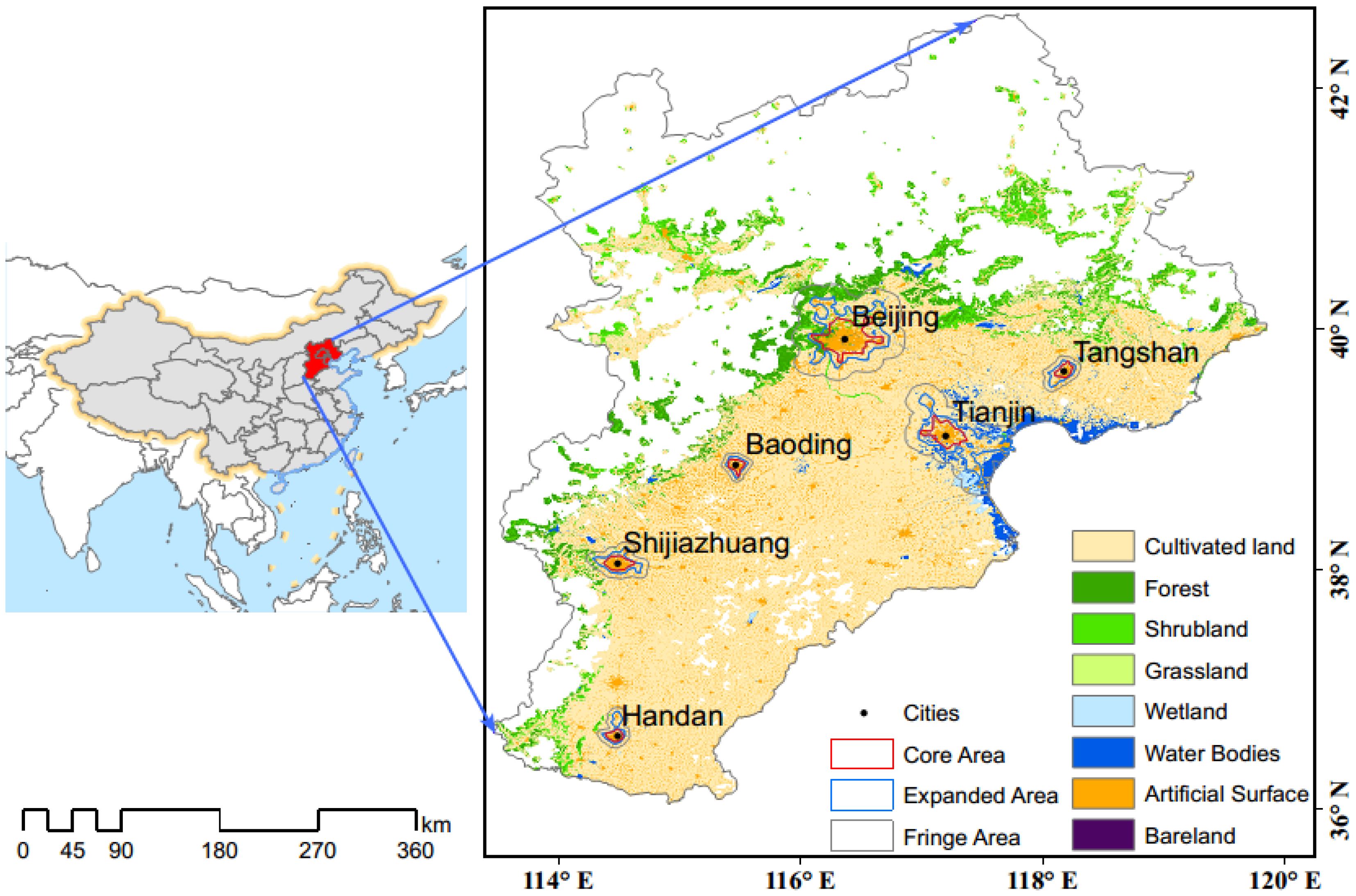
The Jing-Jin-Ji region is located in the North China Plain, with the Bohai Sea to the east and the Taihang Mountains to the west. The altitude is higher to the northwest and lower to the southeast, with a total area of 185,000 km2. The area has a typical temperate monsoon climate that is characterized by rainy summers with high temperatures and cold and dry winters. The fastest population growth period in the Jing-Jin-Ji region is from 2000 to 2010 [46]. The Jing-Jin-Ji urban agglomeration is one of the three major urban agglomerations along the eastern coast of China due to active economic activities. The fast-growing population and rapid urbanization make it a hotspot for urbanization-related scientific research in China [47,48]. To select representative cities, Beijing (BJ), Tianjin (TJ), Shijiazhuang (SJZ), Handan (HD), Tangshan (TS), and Baoding (BD) are chosen, as they have populations greater than one million based on the 2012 China City Statistical Yearbook, in order to identify the differences in albedo for each city during urbanization. The study area is shown in Figure 1, and the GlobeLand30 data for 2000 and 2010 are used for the statistics in this area (Table 1). The results (Table 1) show that the largest decreasing areas were characterized by cultivated land (−6.33%, from 2000 to 2010), while the largest growth areas were characterized by shrub lands (5.42%), followed by artificial land surfaces (1.31%).
Besides, we made a statistic about the typical albedo value for each type of land cover based on the MODIS albedo products from its multiyear average value (Table 1).
Although the albedo mean values exhibit little difference between 2010 and 2000 due to the coarse resolution of albedo (compared to GlobeLand30), we can still see differences among land cover types. So, we just list the typical albedo values in 2010 in the table above, where shrublands have the largest albedo mean value (0.137), and artificial surfaces have a relatively small albedo value which is just bigger than wetland and water bodies.
2.2. Surface Albedo Data Set
The MODIS 16-day 1 km albedo products (MCD43B3, collection5) from 2001 to 2011 were used in this study. The product contains the black-sky albedo (BSA) and the white-sky albedo (WSA), which can be used to calculate the actual (blue-sky) albedo based on the fraction of diffuse skylight [49,50]. Considering the small difference and high correlation between BSA and WSA [44,51,52,53], WSA was used as the index of albedo in this study. MODIS surface albedo products have been validated on a global scale, and the accuracy has been demonstrated to be suitable for studies on climate change [54,55]. We synthesized the 8-d intervals for albedo into yearly scales for the contribution analysis. The corresponding albedo quality data (MCD43B2, collection5) were also used to avoid the effects of snow cover.
2.3. Vegetation Index Data
The monthly MODIS Enhanced Vegetation Index (EVI) product (MOD13A3) with a spatial resolution of 1 km was used. This product was generated based on atmosphere-corrected bidirectional surface reflectance, where the atmospheric effects of water, clouds, and aerosols were removed [56,57]. This product has been widely used in studies regarding global vegetation monitoring, land cover changes, and climate researches [58,59].
2.4. Nighttime Light Data
Nighttime light signals detected by remote sensing satellites derive from the Defense Meteorological Satellite Program (DMSP), specifically from its visible and near infrared sensors named Operational Linescan System (OLS). DMSP/OLS nighttime light data are widely used in research regarding urban areas, such as estimating urban population [60], extracting urban extent [61], measuring urban expansion [62], and exploring human activities and its impacts on the environment in urban areas [43] etc. DMSP/OLS nighttime light data (Version 4) were used in this study, whose spatial resolution is 1 km. We excluded pixels without light (DN = 0) to ensure that there were human activities in every part of our study areas. In addition, an invariant target area method [63,64,65] for image correction was used to perform continuous and saturation corrections on the data. Using this method, we gained a nighttime light data time series with comparable DN values, which have been used to identify the urbanization [44].
2.5. GlobeLand30 Landcover Data
GlobeLand30 is one of the global land cover map products at a 30-m resolution, which was produced with a pixel-object-knowledge (POK)-based operational mapping approach [66]. The classification system includes ten land cover types, namely cultivated lands, forests, shrublands, grasslands, wetlands, water bodies, tundra, artificial surfaces, permanent snow and ice, and barren lands for the years 2000 and 2010. The overall classification accuracy is over 80% [67], and it has been widely validated in many other researches [68,69].
3. Methods
3.1. Urban Area Extraction
Based on DMSP/OLS data, the urban areas in 2000 and 2010 were extracted using a clustering algorithm [61]. Urban core area, fringe area, and rural area are characterized by metropolitan morphology, and urban fringe is a transition zone from urban to rural areas [70,71,72]. In this study, the core areas and the fringe areas are studied in urban expansion. Core Area is extracted by DMSP/OLS in 2000, and it is the place where the central part of the city is located. The area where the fringe area in 2000 turned into the core area in 2010 was named the Expanded Area. In order to identify this urban sprawl process of each city, the Expanded Area was defined as the urban area extracted in 2010 (excluding the Core Area). The Fringe Area in this study was defined as the buffer zone whose areas were equal to the urban areas extracted in 2010 (Figure 1). The Core Area, Expanded Area, and Fringe Area can represent not only the old urban area, the new urban area, and the suburbs, but also the initial stage, middle acceleration stage, and final stage of the urbanization process, respectively.
3.2. Breakpoint Analysis
A shift linear analysis method [42,73] was used to identify the breakpoint in the albedo time series. The idea behind this method is determining the point where the slope changes significantly in the time series before and after the point. The calculation method is as follows:
where denotes the albedo in the ith year; denotes the ith year; and and are the fitted parameters. Among them, and represent the slopes of the fitted line, represent the fitted intercepts, and represents the breakpoint position.
The Chow test which is generally used to detect changes in time series was applied to test the significance in this study and the formula is expressed as follows:
where indicates the sum of square errors of the time series. For the former number of the time series, indicates the sum of square errors of the former time series, and indicates the sum of square errors of the latter number of the time series. c is the number of the estimated parameter in the whole time series.
3.3. Interannual Variation Rate Calculation
A simple linear regression model was used to calculate the interannual variation rate. Using the albedo time series as an example, the interannual variation rate of each pixel is equal to the slope of the trend line via the least-squares regression of the multiyear value in each pixel. The calculation for the slope is as follows:
where represents the interannual variation rate of albedo, n represents the number of years, i denotes the ith year, and denotes the albedo value in the ith year. A positive slope value indicates an increasing trend, while a negative slope indicates a decreasing trend.
The significance of the calculated tendency is determined by an F test. The calculation formula is expressed as follows:
where indicates the sum of square errors, and represents the regressed square sum. denotes the albedo value in the ith year, denotes the albedo regression value in the ith year, denotes the mean albedo value across all years, and n denotes the number of years.
This method has also been applied to the calculation of interannual variation rates for vegetation and urbanization, where and represent the interannual variation rate of vegetation and urbanization, respectively.
3.4. Contribution Analysis
Urbanization and vegetation are two main factors that affect variations in albedo. In our study, the annual variation rate of albedo in each pixel is expressed by the contributions of vegetation (V), urbanization (U), and other factors () (formula (5)).
where represents the interannual variation rate of albedo. C(V), C(U), and C() represent the contributions of vegetation, urbanization, and other factors to the interannual variation rate of albedo, respectively. The vegetation contribution calculation method [74] is as follows:
represents the slope of the linear regression line for the multiyear EVI time series. A denotes albedo, V denotes EVI, and (S(V)) represents the sensitivity of albedo to EVI. This sensitivity term was derived as a partial derivative via the multiple regression of albedo on EVI and DMSP/OLS. Positive and negative values of this sensitivity term reflect the positive and negative correlations between the analyzed factors and albedo, respectively. The magnitude of the absolute value of the sensitivity coefficient indicates whether the relationship between the factors and albedo is strong or weak (the greater the value, the stronger the relationship). The contribution of urbanization (C(U)) can also be calculated via the sensitivity of albedo to urbanization(S(U)) and KU in the same way.
Due to the spatial differences in the contribution intensity from vegetation and urbanization in different regions, the relative contribution percentage of vegetation, urbanization, and other factors to changes in albedo can be expressed with the following equation [44]:
where, and P(∆) represent the relative contribution percentage of vegetation, urbanization, and other factors, respectively.
P(∆)=100 − P(V) − P(U)
4. Results
4.1. Albedo Variations and Spatial Patterns
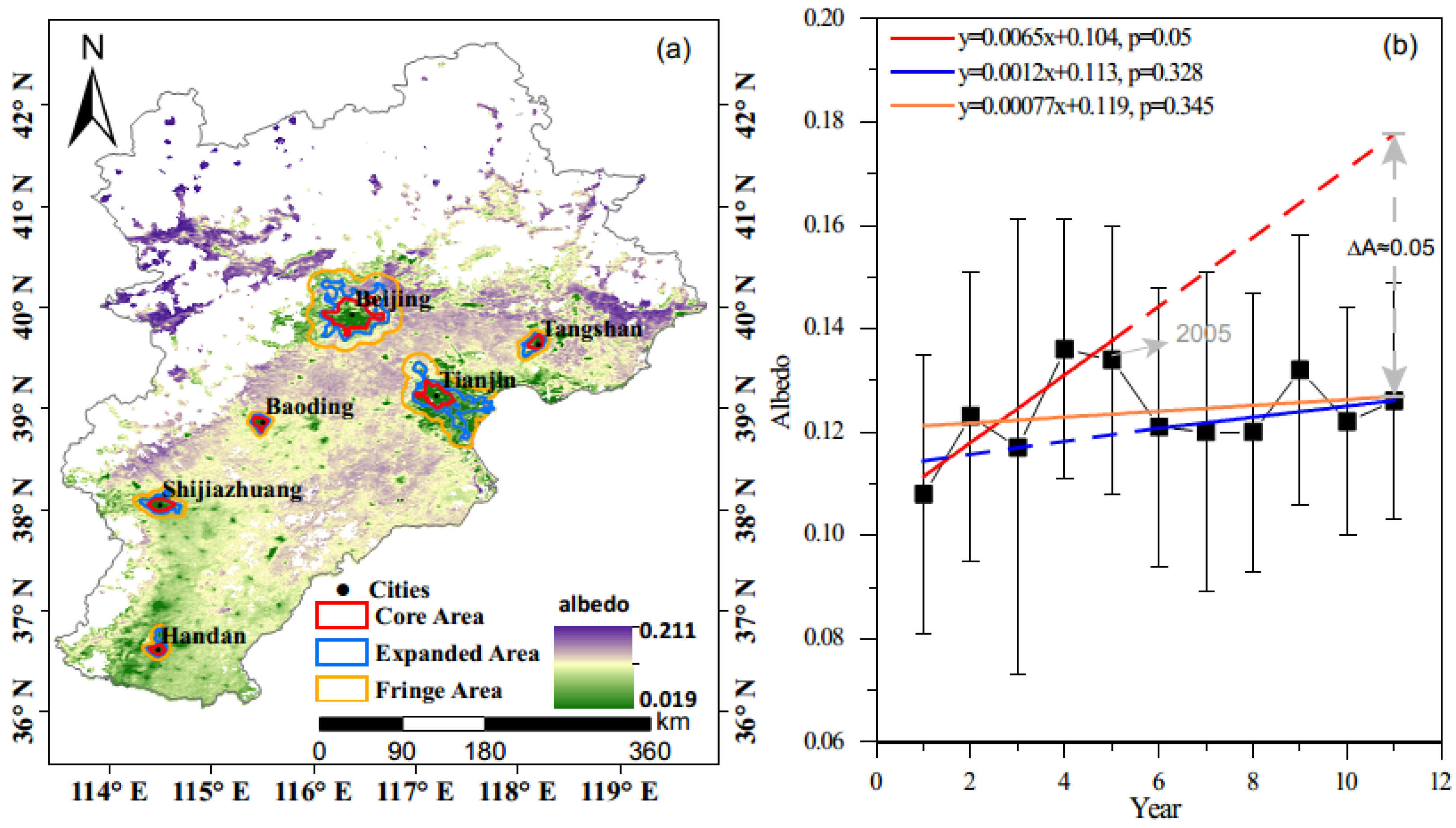
The average albedo of the Jing-Jin-Ji region from 2001 to 2011 was 0.12 ± 0.02 and the spatial distribution of the multiyear mean albedo is shown in Figure 2. According to this spatial pattern, the albedo increased from the Central Business District (CBD) to the suburbs, and a majority of the Core Area had the lowest mean value of albedo compared to that in other areas. Based on the shift linear regression method [42], the results of the breakpoint detection showed that 2005 was the breakpoint year for the ~10 years of albedo data. With the Chow test, the p-value of the breakpoint detection was 0.002, which was substantially less than 0.05 and significant. The trend in albedo from 2001–2005 (T1 period) was the highest (6.5 × 10⁻³ year−1, p < 0.05), with a lower trend of 1.2 × 10⁻³ year−1 (p > 0.05) from 2006–2011 (T2 period), whereas the lowest trend occurred from 2001–2011 (T3 period; 0.78 × 10⁻³ year−1 at p > 0.05). These trends show big differences in the T1 and T2 periods. The albedo trend during T2 was approximately 1/5 the trend during the T1 period, which led to a reduction in albedo of approximately 0.05. This indicates that the long-term growth trend of albedo was suppressed after 2005 due to several influential factors.
To identify the factors contributing to this difference, we explored the spatial patterns of albedo before and after the breakpoint (Figure 3).
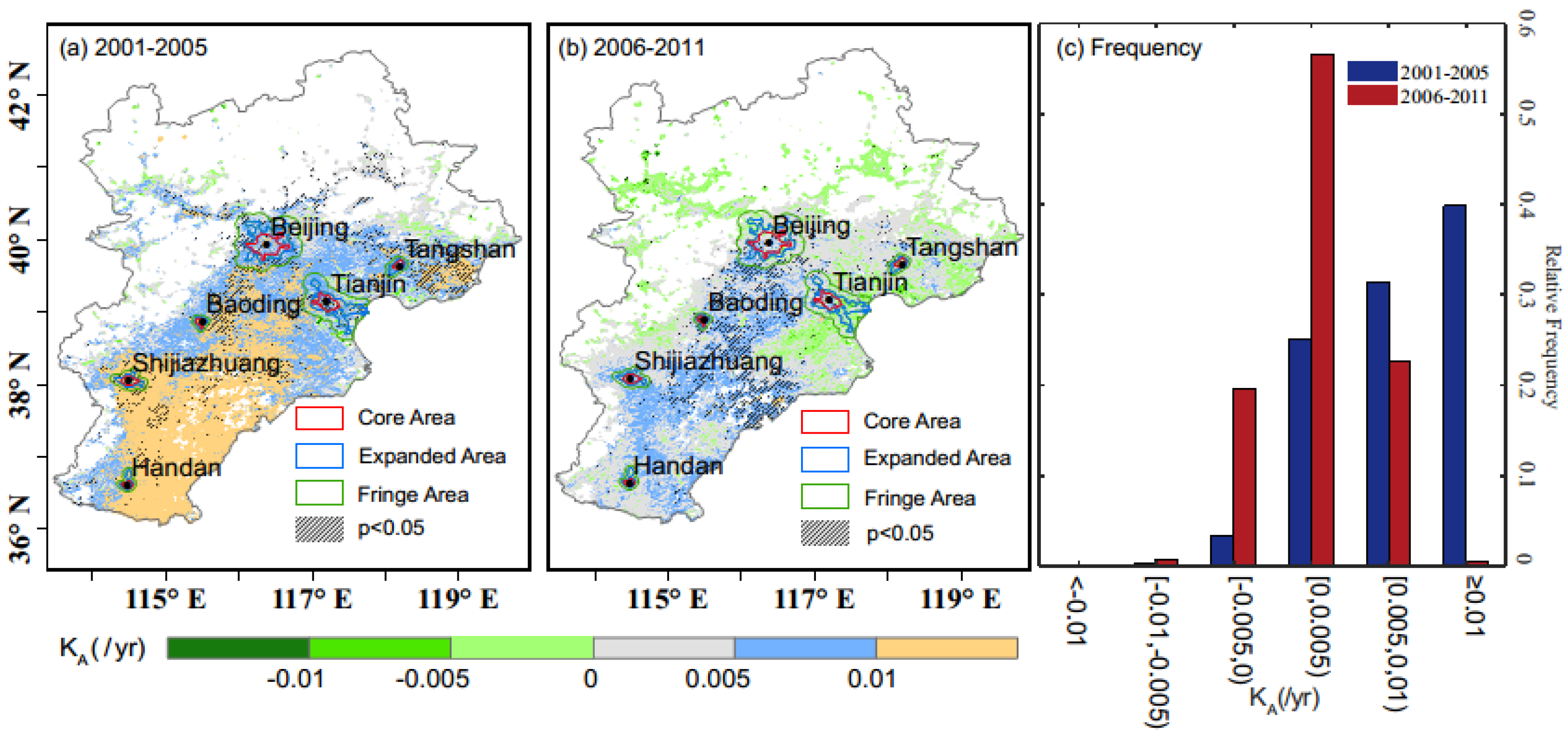
From 2001–2005 (Figure 3a), the albedo showed an increasing trend (k > 0) in over 99.5% of the whole region, while the number of pixels with a decreasing trend (k < 0) in albedo was small and accounted for only 0.5% of the total area. The percentage of the area where the albedo had significant trends (p < 0.05) is 13.2%, in which the percentage of the significant increasing trend (p < 0.05) was 13.13% and the significant decreasing trend (p < 0.05) was 0.07%. Albedo showed a general increasing trend in the study area. Spatially, from southwest to northeast, the interannual variation rate of albedo gradually decreased. Pixels of decreasing trends were mainly distributed across the northern fringe areas and along east coast areas near Bohai Bay.
From 2006–2011 (Figure 3b), the albedo generally had a lower increasing trend than that in 2001–2005. The percentage of the area of increasing albedo trends decreased to 94%. In addition, the area of decreasing albedo trends increased, which accounted for 6% of the total area, distributed in the northern and eastern coastal areas. The area of significant albedo trends (p < 0.05) was 11.11%, in which the area of increasing trends (p < 0.05) took up 10.44% of the whole area and the area of decreasing trends took up 0.67%.
4.2. Urbanization Spatial Patterns
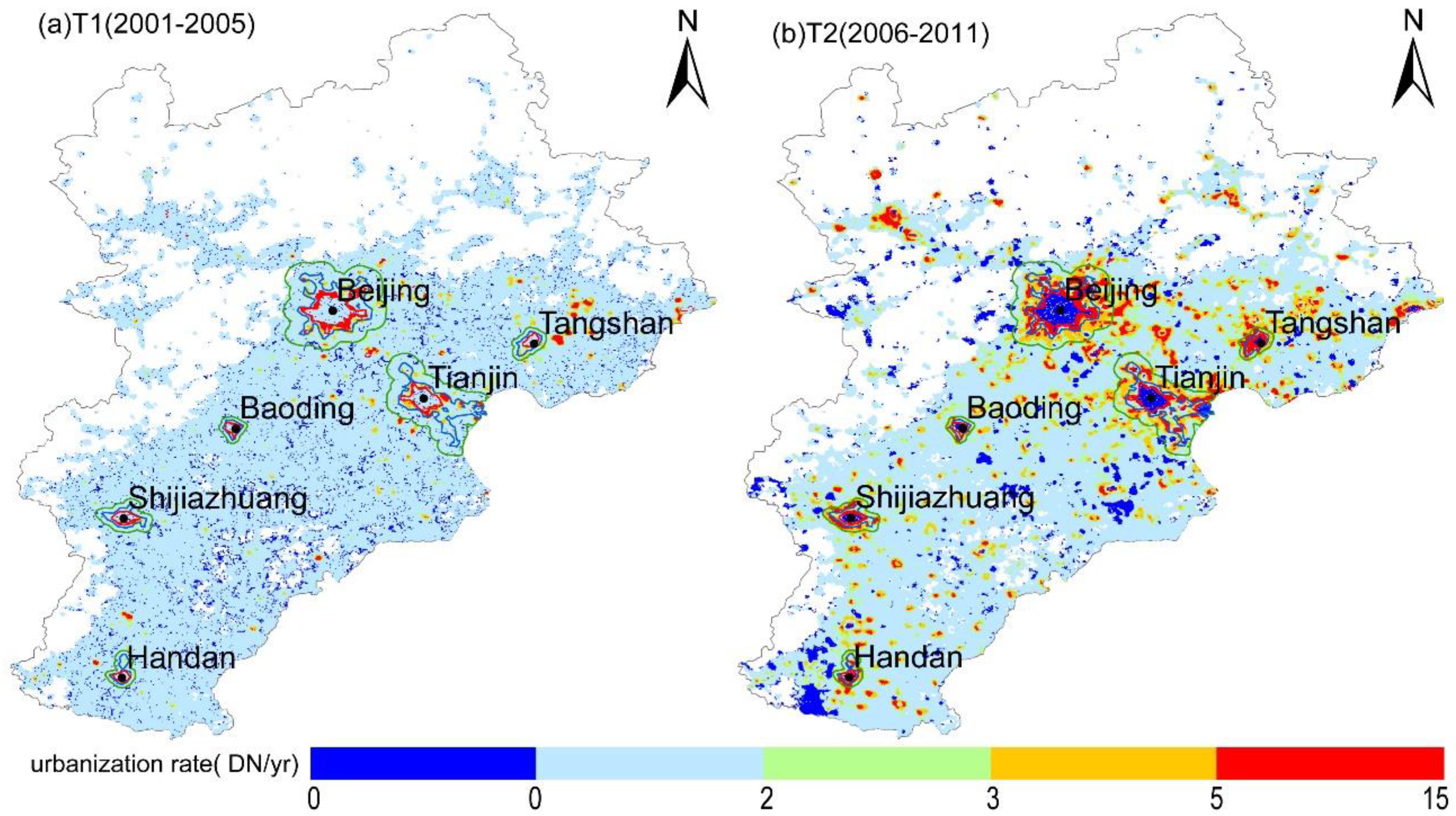
In this study, we use the interannual variation rate of the DN values from corrected DMSP/OLS nighttime light data to define the urbanization rate (Figure 4) and study the developmental characteristics in the Jing-Jin-Ji region during T1 and T2 periods.
From 2001 to 2005 (Figure 4a), the urbanization rate in most parts of the Jing-Jin-Ji region was less than 2 year−1, and the urbanization rate in only a few areas of the Expanded Area surrounding Beijing, Tianjin, and Tangshan was greater than 5 year−1. After 2005 (Figure 4b), although the rate of urbanization in the urban Core Area almost decreased to 0, the rate of urbanization in other areas increased significantly, and the urbanization area increased significantly, indicating that there is rapid urbanization occurred after 3 April 2005.
4.3. Sensitivity of Urbanization and Vegetation to Albedo
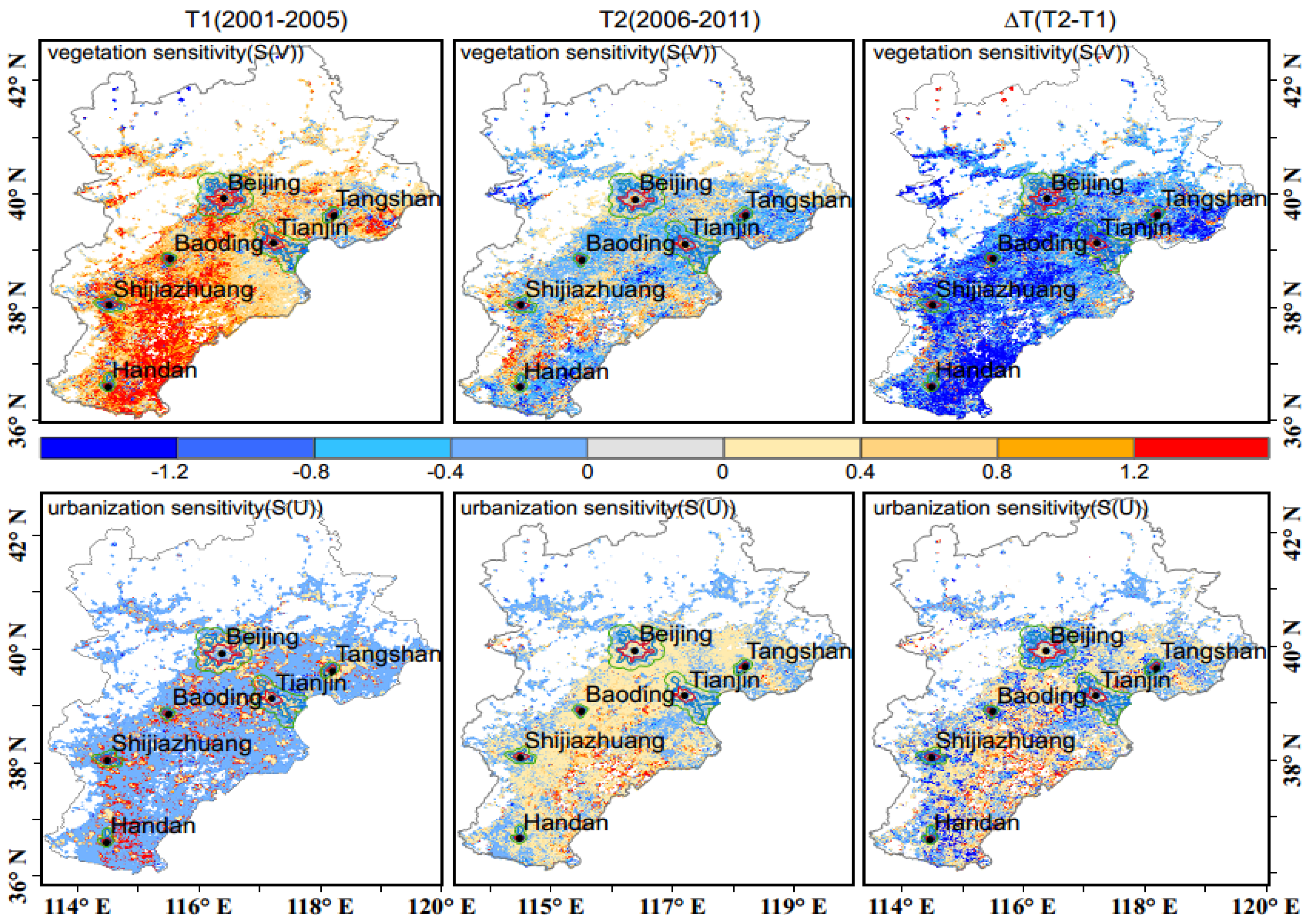
Numerous studies have shown that vegetation and urbanization are two major factors that cause changes in surface albedo [21,75]. For vegetation, different types of vegetation have different levels of albedo. For example, forests usually have a lower albedo (0.05–0.2) while grasslands have a higher albedo (0.16–0.26) [76]. In addition, changes in surface roughness caused by vegetation growth are also responsible for changes in albedo. In a similar way, surface roughness also changed with the process of urbanization. Land cover changes in the process of urbanization play a decisive role in the properties of three-dimensional surfaces in urban areas, which equally has a decisive influence on albedo in urban areas. The three-dimensional surfaces formed by buildings and roads etc. create large inner spaces and cracks for lights to transfer, which result in the multiple reflection of lights, trapping lights, and leading to a decrease in albedo. Considering that the units of vegetation data and nighttime light data are not uniform, and the range of values for these data is quite different, the corrected DMSP/OLS data in this study has been normalized. The sensitivity of albedo to vegetation and urbanization intensity is calculated by multiple linear regression. The spatial distribution patterns of each factor’s sensitivity term during different periods, as well as their variations, are shown in Figure 5. The sensitivity of albedo to vegetation and urbanization displays differences in period T1 and period T2.
In period T1 (2001–2005), the sensitivity of albedo to urbanization showed a significant spatial distribution difference, of which the fifth percentile was −0.006 and the 95th percentile was 1.95. Spatially, the relatively high positive S(U) is mainly concentrated in the surrounding areas of major cities, such as Beijing, Tianjin, and Tangshan, positive-correlated to albedo. In contrast, S(U) in other regions is much smaller and generally negative, which has a weak negative correlation with albedo. In these regions, the sensitivity of albedo to vegetation(S(V)) shows high positive sensitivity, especially in the southeastern plains. In summary, urbanization has stronger promoting effects on albedo around large cities and has much weaker suppressing effects on albedo in other regions, where vegetation plays a promoting role in these areas.
In period T2 (2006–2011), instead of concentrating in areas surrounding large cities, the sensitivity of albedo to urbanization shows a regional diffusion feature compared to that in T1. In total, 72% of the S(U) is positive, and the fifth percentile of S(U) is −0.24 and the 95th percentile is 0.73. As the sensitivity of urbanization increases over a large area, the sensitivity of vegetation decreases significantly and extensively. In total, 53% of the vegetation sensitivity(S(V)) shows negative effects and mainly ranges from −0.4 to 0 (i.e., vegetation tends to inhibit the increase in albedo during this period).
From T1 to T2, the sensitivity of albedo to vegetation generally decreases and changes from positive to negative. The effect that this change causes is that the strong increased effect of vegetation on albedo turns into a weak decreased effect. However, the sensitivity of albedo to urbanization has extensively increased. The increased effects of urbanization on albedo exist not only in areas surrounding large cities during T1, but also in other large areas during T2, although the sensitivity intensity is much larger in T1 than that in T2.
4.4. Effects of the Influential Factors on Changes in Albedo
The sensitivity of albedo to vegetation and urbanization indicates a correlation between albedo and various factors. Because it is dimensionless, this correlation does not quantify the effects of various factors on albedo. Therefore, our study also quantifies the effects of vegetation and urbanization on albedo based on sensitivities. The effects of each factor on the interannual variation rate of albedo are shown in Figure 6.
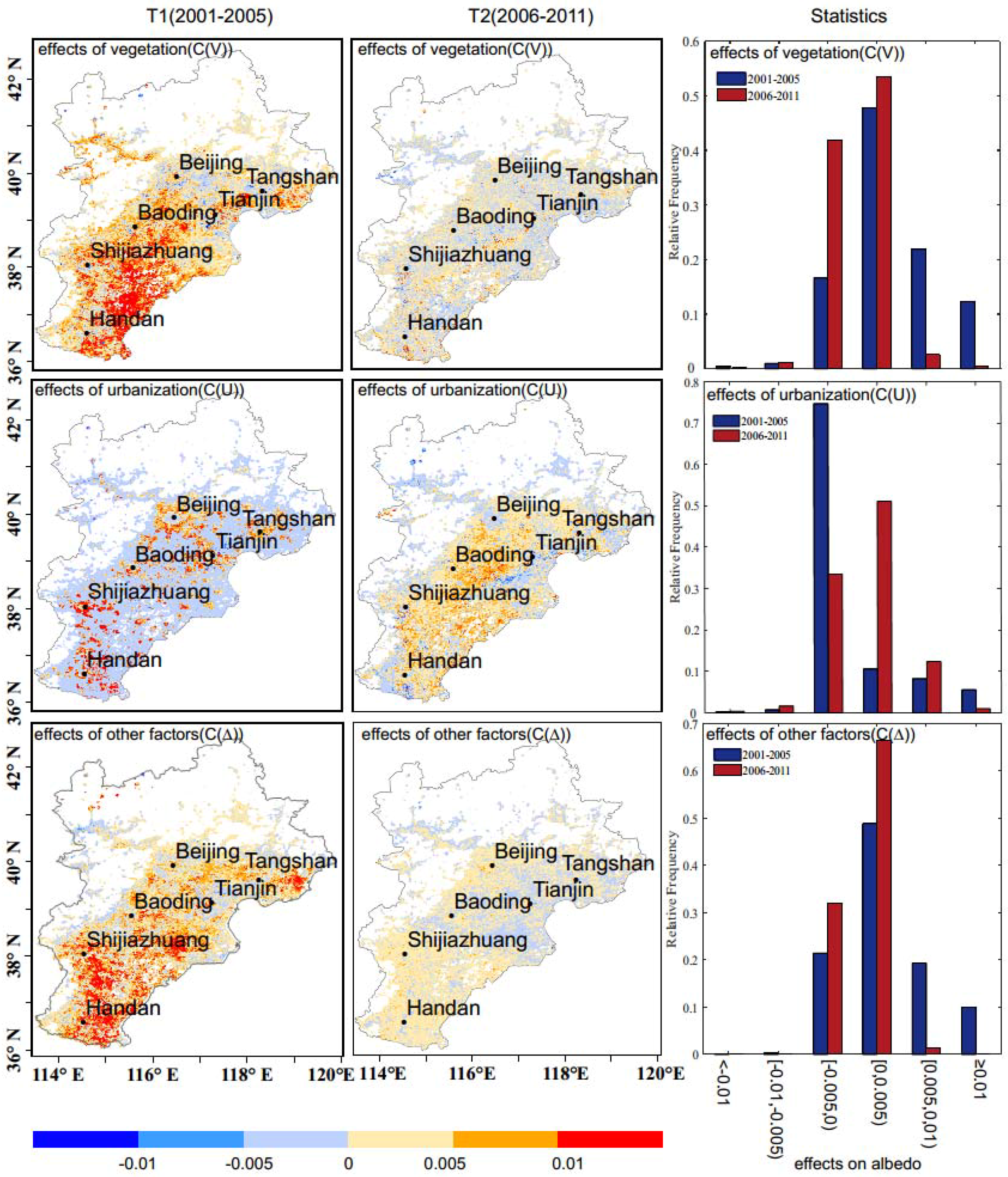
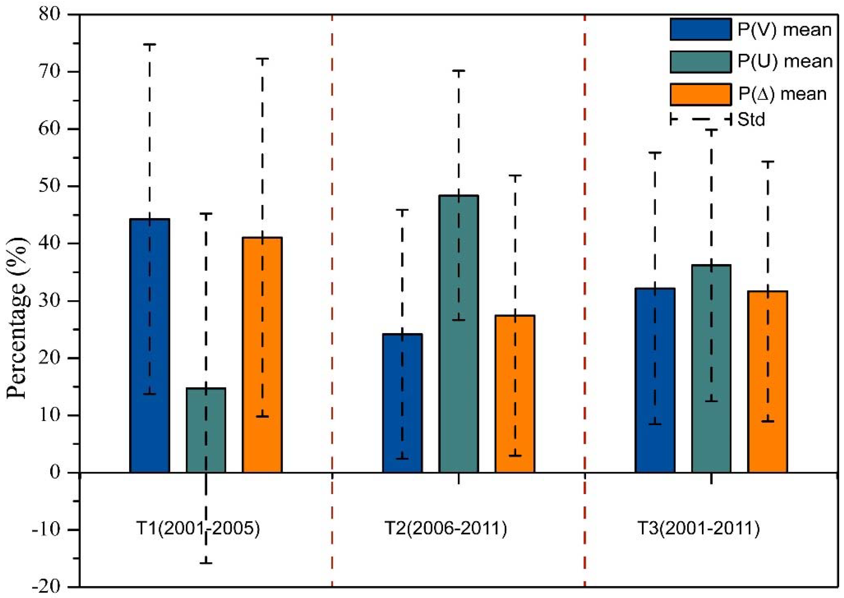
From 2001–2005, the area with positive effects of vegetation on the interannual variation rate of albedo comprised more than 80% of the entire region (Figure 6). The areas with negative effects of vegetation mostly existed in the surrounding areas of cities and partially in the northern area of the study region. Urbanization had extensive positive effects on albedo, which were distributed around large cities. Shijiazhuang, Handan, and their surrounding areas had greater positive effects on variations in albedo compared to those from Beijing, Tianjin, and Tangshan, with the greatest effects exceeding 0.01 year−1. The effects in other regions were almost 0. Other factors had both positive and negative effects on variations in albedo, but most of these effects were positive and located in Shijiazhuang, Handan, and their surrounding areas, with effects greater than 0.01 year−1. In the northern part of the region, the effects of other factors on albedo were almost in the range of −0.005 to 0.005 year−1. The statistics of the relative contributions of each factor (Figure 7) show that from 2001–2005, the relative contribution percentage of vegetation, urbanization, and other factors was 44%, 15%, and 41%, respectively. Urbanization had the lowest contribution to regional albedo, whereas vegetation and other factors were the two main controlling factors in variations in albedo, which were both greater than two times the amount of contribution from urbanization. One thing that must be explained is that due to the type and distribution differences of each factor, the spatial heterogeneity was relatively obvious. As a result, some pixels were under the absolute control of vegetation, and some were under the absolute control of urbanization, which led to an expected large standard deviation (STD) value for each factor’s contribution.
From 2006–2011, the effect of vegetation on variations in albedo mainly ranged from −0.005 year−1 to 0.005 year−1, which was generally lower than that from 2001–2005 (Figure 6). Over 99% of the urbanization effects on albedo were positive. The areas effected by urbanization expanded although the value of this effect decreased compared to the urbanization effect from 2001–2005. The effect of other factors was distributed uniformly across the study area, ranging from −0.005 to 0.005. From 2006–2011, the relative contribution percentages of vegetation, urbanization, and other factors to albedo (Figure 7) were 24%, 48.5%, and 27.5%, respectively. Urbanization became the highest contribution factor, which increased by more than 200%. In contrast, the contributions from vegetation and other factors decreased by 20% and 13.5%, respectively.
The relative contribution percentages of vegetation, urbanization, and other factors to albedo are different not only in size, but also in spatial distribution pattern (Figure 8).
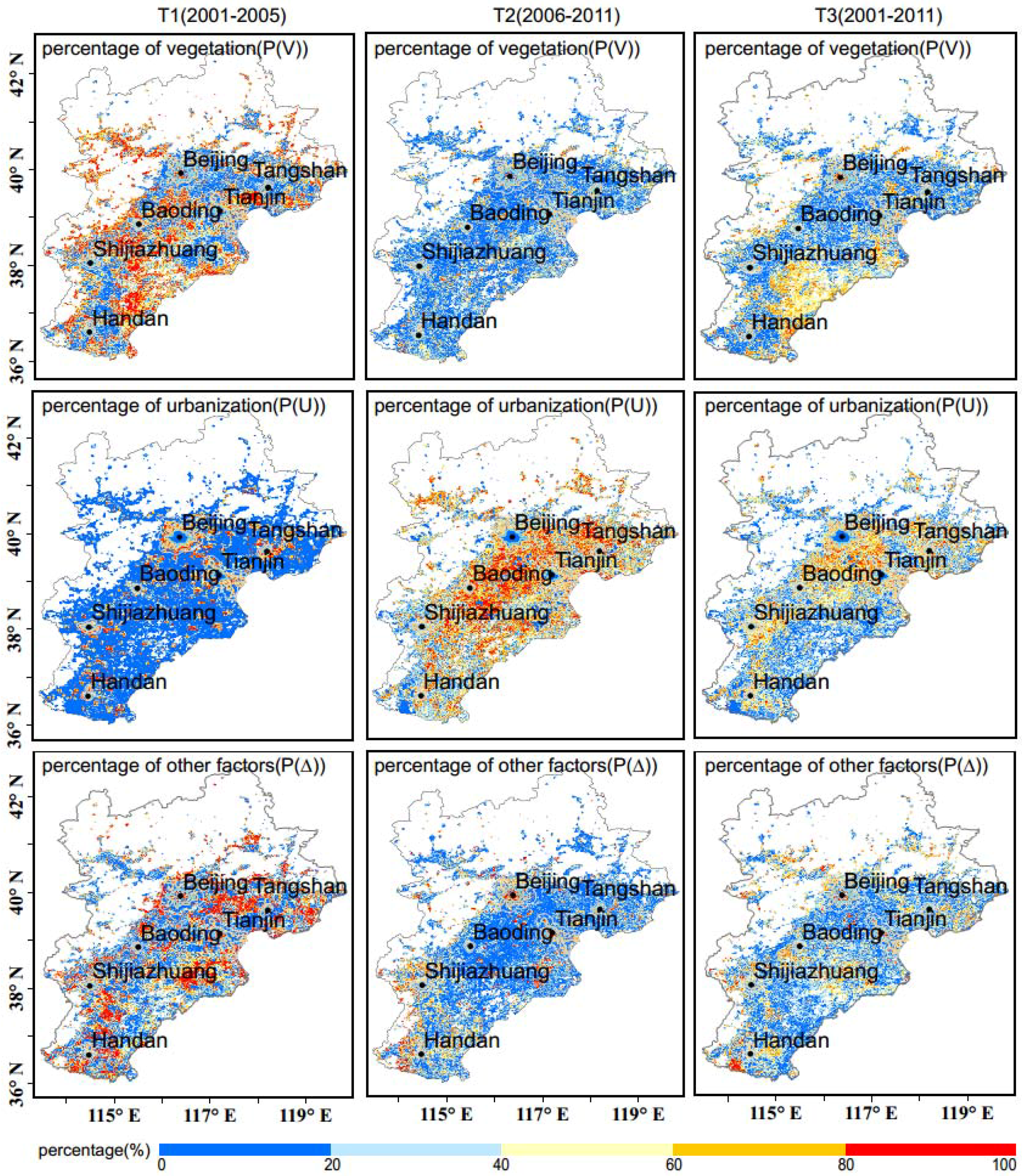
Although the relative contribution percentage of each factor for the whole region is approximately 30% from 2001 to 2011 (Figure 7), the dominant controlling factors are different in different regions (Figure 8). From 2001–2011, the variations in albedo were mainly controlled by vegetation in the southeast and parts of the eastern region. Other regions were mainly controlled by urbanization, especially in regions surrounding cities, except for the Core Area, which was largely affected by both vegetation and other factors. From 2001–2005, the locations where the urbanization contribution was greater than 60% were the Expanded Area and the Fringe Area, while other regions were mostly controlled by vegetation. Other factors playing dominate roles were distributed in the triangular region formed by Beijing, Tianjin, and Tangshan, as well as near the connecting line between Shijiazhuang and Handan. From 2006 to 2011, the contributions of vegetation and other factors showed a significant reduction. The contribution percentage of vegetation was generally lower than 20%, whereas the contribution percentage of urbanization increased substantially in other regions (generally greater than 60%), except for the Core Area, where the urbanization contribution percentage was equal to zero. Other factors mainly affected the changes in albedo in the Core Area and a partial region near the connecting line between Shijiazhuang and Handan.
4.5. Urbanization in Representative Cities
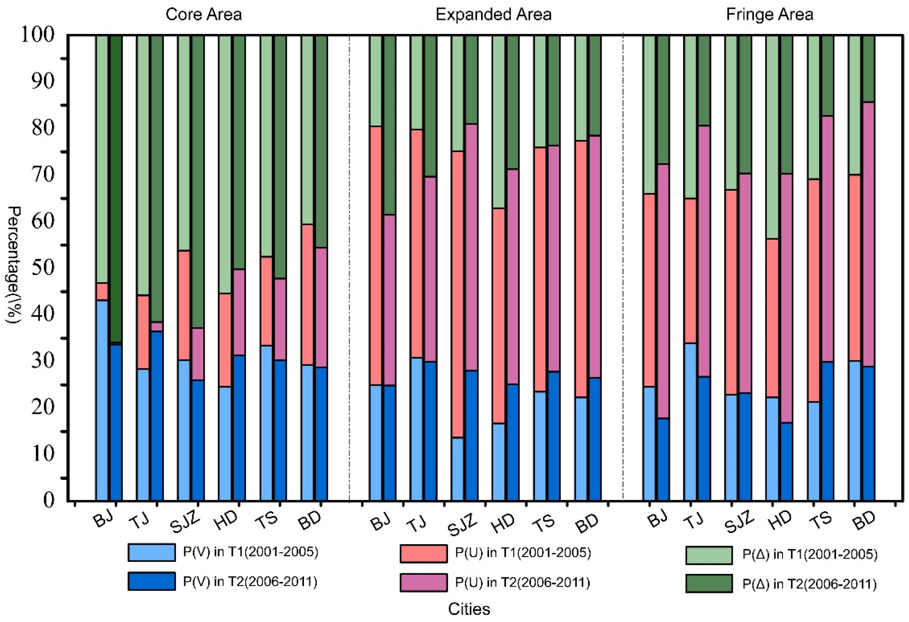
According to the above analysis, urbanization transformed from a secondary influential factor from 2001–2005 into a major influential factor from 2006–2011, indicating that the effect of urbanization on regional albedo has increased since the breakpoint year (2005). However, the urbanization intensity of each individual city is substantially different. The Core Are, Expanded Area, and Fringe Area in our study represent the initial stage, middle acceleration stage, and final stage of the urbanization process, respectively; why is albedo different during these different urbanization stages? What are the main controlling factors for these areas? Are there any regional differences among the impact factors? We still do not know much about these issues. Therefore, in this paper, we also calculate the relative contribution percentages of vegetation, urbanization, and other factors in different functional areas (Figure 9).
For each individual city, the variations in albedo in Core Areas are mostly affected by other factors (Δ), followed by vegetation, and the contribution of urbanization is minimal. The average contribution percentages of vegetation, urbanization, and other factors are 34.5%, 8.4%, and 57.1%, respectively, in the Core Area. This result indicates that because the Core Area is generally composed of old cities that have generally completed urbanization, the influence of human activities on the variations in albedo is basically at a stable level; therefore, the urbanization contribution to albedo (8.4%) is much smaller than the contributions from other factors and vegetation. In the Core Area of the six major cities, other factors contribute more during T2 than those during T1 in 84% of our cities. Vegetation contributes more during T2 than that during T1 in 67% of our cities. The urbanization contribution decreases during T2 compared to that during T1 in 100% of our cities. It is safe to say that the contributions from vegetation and other factors in the Core Area will increase with time, while the contribution from urbanization will decrease.
In the Expanded Area, the average contribution percentages of vegetation, urbanization, and other factors were 26.5%, 46.7%, and 26.8%, respectively, and urbanization was the most important contribution factor in the Expanded Area. Spatially, compared to the Core Area, urbanization had the greatest change in the Expanded Area, with an increase of 456%; the contributions of other factors and vegetation decreased by 53% and 23%, respectively. Temporally, the urbanization contribution percentage decreased to various degrees during T2 compared with that during the T1 period. Meanwhile, the vegetation contribution percentage increased in 67% of the cities, while the contribution percentage of other factors decreased. However, Beijing and Tianjin, whose populations are greater than five million, showed the opposite effect; that is, the vegetation contribution percentage decreased slightly in the Expanded Area, while the contribution of other factors increased significantly. For small cities, urbanization accompanying land cover change might have been finished in the Expanded Area and there would be no land cover changes for several years at least in the future, due to the limited population and limited population increasing ability. So, the number of the residents living in this area is relatively stable, which could lead to the stable growth of the vegetation and green space for a comfortable living environment. Thus, the contribution of vegetation will increase. On the contrary, for Beijing and Tianjin, which are the two biggest cities in the Jing-Jin-Ji area, they have been maintaining a fast-speed of urbanization for a long time. With reference to the Globeland30 land cover maps, we know that land cover changes are still happening, and they happened in the Expanded Area. That is to say, the urbanization process is going on in Expanded Areas in Beijing and Tianjin. So, due to the limited urban space, the rate of green space to urban space in Beijing and Tianjin would be smaller than small cities. Thus, the contribution of vegetation in Expanded Area in these big cities is relatively small compare to those in small cities.
In the Fringe Area, the average contribution percentages of vegetation, urbanization, and other factors were 24.9%, 45.8%, and 29.3%, respectively. Compared to the Expanded Area, the urbanization contribution percentage in the Fringe Area decreased, but it was still the dominant contribution factor. However, the vegetation contribution percentage decreased, and the contribution rate of other factors increased. Temporally, the contribution percentage of urbanization increased significantly from period T1 to period T2, and the contribution of other factors decreased significantly. The vegetation contribution percentage also slightly decreased in most of the cities.
In summary, from the Core Area to the Fringe Area, the spatial urbanization contribution percentage rapidly increases at first, followed by a slow increase. The vegetation contribution percentage rapidly declines during period T1, while it slowly declines during period T2. The contribution of other factors decreases quickly during period T1, but slowly increases during period T2. Temporally, the urbanization contribution in the Core Area and the Expanded Area decreases over time, whereas the contribution of vegetation increases. In the Fringe Area, the urbanization contribution increases rapidly with a rapid decrease in vegetation contribution. The other factors only have a significant increase in the Core Area, with decreasing trends in the Expanded Area and Fringe Area.
5. Discussion
In our study, nighttime light data were corrected to characterize the changes in urbanization intensity by the DN value and various functional regions of the city were extracted to express the various stages of urbanization. Combined with the vegetation index data, we quantitatively analyzed the contribution of urbanization and vegetation to variations in albedo. The contribution analysis method used in this study is a partial derivative method, which is widely used in studies on the effects of climate on hydrological dynamics [77,78] and studies on climate response [74,79]. Based on the results of this quantitative analysis, we concluded that the significant increase in the urbanization contribution and the decrease in the vegetation contribution after 2005 were the main reasons for the significant decreasing growth rate of albedo after 2005. In terms of mechanisms, this was consistent with previous conclusions on urban albedo; that is, urbanization could cause a decrease in albedo, which is generally correlated to the surface roughness. For example, albedo observations based on model experiments from Aida [16] showed that multiple reflections of solar radiation in urban canyons increased the absorption of solar radiation in cities, resulting in a reduction in urban albedo. Kondo [80] used the Monte Carlo ray tracing method to show that building height affects albedo, and low-rise buildings have a high albedo. The impact of urban areas, which are one of the most densely populated areas, on urban albedo is multi-fold [81,82,83,84]. On one hand, urbanization is accompanied by changes in land cover. In general, the process of transition from a village to a city involves replacing natural surfaces (e.g., farmlands and forests) with impervious surfaces (e.g., cement and asphalt). Due to the changes in the thermal conductivity of the Earth’s surface, albedo changes, and the water and heat exchange between the Earth’s surface and the atmosphere also changes. The 3D solid surface formed during urbanization has resulted in an increase in surface roughness [16,76,80,85,86] and solar radiation absorption [77], which share the same mechanism with soil roughness and soil albedo. Inner spaces enable the multiple reflection of lights, which increases the absorption of radiation. For this reason, urban areas usually have low albedo [8]. The multiyear average of reflectivity calculated by MODIS albedo products also showed this rule; that is, that albedo in urban areas is generally low (Figure 2). On the other hand, the ability of cities to attract people is also obvious. Urban areas account for approximately 0.5% of the total land area in the world, but they accommodate more than half of the world’s population [87]. Due to the complexity and uncertainty of the human activities during the urbanization process, it is very difficult to identify the urbanization effects. The DN value of the night-time lights data is used as the index of urbanization intensity, which could show comprehensive impacts of human activities. This enables us to simplify the impact of urbanization on albedo changes and helps us to quantify the contribution of urbanization and vegetation to the changes in albedo from a macro perspective.
As the parameter indicating the surface’s ability to reflect solar radiation, albedo plays a key role in the energy balance at the surface, and the effects of albedo on climate change have raised substantial attention from many scholars. Akbari et al. [88] simulated the long-term effects of urban albedo growth using a mesoscale complex global climate model (UVic Earth System Climate Model), and it was believed that an increase in surface albedo by 0.01 over a square meter could reduce the long-term global temperature by 3 × 10⁻⁵ K, which was equivalent to reducing CO2 emissions by 7 kg [89]. Sailor [8] analyzed the surface albedo in Los Angeles based on a three-dimensional meteorological model and found that albedo increased by 0.14 in urban regions and 0.08 in basin areas, which could reduce the maximum heat by 1.5 °C in summer. Based on a mesoscale atmospheric model, Humdi [40] analyzed the intensity of UHIs and found that the increase in albedo over three types of urban surfaces (walls, roofs, and roads) could reduce the UHI both during the day and at night. Wang et al. [89] analyzed the impact of land use change in urban regions on extreme heat events with the Weather Research and Forecasting model (WRF) in Jing-Jin-Ji and found that an increase of the albedo on urban roofs from 0.12 to 0.85 could reduce the urban mean temperature by 0.51 °C, which was equivalent to 80% of the heat caused by urban expansion in the last 20 years. Menon [7] increased the albedo of roofs and roads using the GEOS-5 basin surface pattern, and the result showed that increasing the albedo of roofs and roads by 0.25 and 0.15, respectively, could result in approximately 57 Gt of CO2 from global urban regions. Compared with the aforementioned study, it is clear that the decrease of albedo (approximately 0.05) in the Jing-Jin-Ji region, caused by the increasing urbanization contribution and the decreasing contribution of vegetation over 2001–2011, is in a relatively reasonable numerical range, and the effects of this variation in albedo on urban temperature are not negligible. Urbanization could change both the urban morphology and the urban environment. Energy-budget parameters are also varied during this process. The heat-trapping morphology of the 3-D surface and the reduced areas of vegetation and water bodies both contribute to albedo variation and could result in urban climate change [82,90]. The decrease of the albedo (~0.05) in our result showed that there might be a high possibility of temperature changes due to urbanization, and it could also affect the UHI in this area. In this way, the difference between the vegetation and urbanization contribution to albedo might be useful in urban planning to mitigate the intensity of the UHI, and helps to offer better comfort conditions to residents [91,92,93].
Because of the significant influence of albedo on temperature in urban areas, increasing the albedo in urban areas to mitigate the urban heat island intensity has become an important aspect of urban energy conservation research. Taha [94] found that the changes in urban albedo via whitewashing could save 35% of the cooling peak power and 62% of the cooling energy. The research of Akbari [95] also showed that urban trees and high albedo could potentially reduce air conditioning energy by 20%, which would save about $10 billion a year in energy costs and help improve urban air conditions. Therefore, it is necessary and meaningful to understand the reason why urban albedo changes during the process of urbanization, which would be helpful for future studies on urban climate change and for the development of urban energy conservation strategies.
There have been many detailed studies on the factors that may influence albedo, such as the solar zenith angle [16], the underlying surface regime [21], soil moisture [96,97], and meteorological conditions [98,99,100]. Based on a mathematical statistics method, our study quantitatively calculated the contributions of multiple factors to urban albedo in each pixel and identified the main contribution factors, which is one of the highlights of our study. However, our study is still insufficient. Because the basis of the calculation method in our study was a comprehensive differential equation, we cannot evaluate the uncertainty of the results. Instead, we can only compare the results with other studies or use other auxiliary data to validate the reliability of our conclusions. Second, one of our study conclusions was that the contribution of albedo in the Expanded Area that also includes the new urban areas and in the suburb-located Fringe Area was mainly affected by urbanization. Since our study simplified the urbanization process, more specific reasoning, such as why urbanization is the dominant factor, still requires more detailed scientific research in the future. Third, we used the DN value of the DMSP/OLS nighttime light data to represent the urbanization intensity, but whether or not this index can assess urban development levels accurately has not been evaluated. In addition, there are many types of nighttime light correction methods, but the methods used in Cao [63] were applied in this study due to the adequate correction effect and more applicable study area (China). However, whether or not this method can be applied at a global scale remains to be explored. Finally, as we have only taken the fastest population growth period (~10 years) into consideration, the length of the time series is relatively short. Therefore, the impact of data length still needs to be evaluated.
6. Conclusions
Based on remote sensing data, we explored the spatiotemporal distribution patterns and variation characteristics of albedo in the Jing-Jin-Ji region. In addition, a quantitative approach based on partial derivatives was applied to calculate the contribution of urbanization and vegetation to albedo variability.
The results showed that albedo changed greatly before and after 2005. Albedo variation was mainly contributed by vegetation (44%) and other factors (41%) before 2005. However, after 2005, large-scale urbanization became the main controlling factor that affected the change in albedo, with a contribution proportion of 48.5%, and the vegetation and other factors contributions were 24% and 27.5%, respectively. Spatially, the contribution percentage of urbanization gradually increased from the Core Area to the Fringe Area, and the contribution percentage of vegetation gradually decreased. Temporally, the contribution of urbanization in the Core Area and Expanded Area decreased with time, and the contribution of vegetation increased. In contrast, the impact of urbanization in the Fringe Area increased, while that of vegetation decreased. Other factors (e.g., extreme weather, natural disasters et al.) contributed more to albedo variation in Core Areas than other areas, and exhibited an increasing trend over time.
In summary, our paper provides a method via mathematical statistics to quantitatively estimate the contribution of urbanization and vegetation to albedo changes in urban areas. Understanding the spatiotemporal differences in albedo via dominant factors will help us perform additional research on urban climate change, especially regarding temperature changes in urban areas. At the same time, it can also provide a data foundation for developing urban energy conservation policies.
Author Contributions
R.T. and X.Z. conceived of and designed the experiments. R.T. processed and analyzed the data. All authors contributed to the ideas, writing, and discussion.
Funding
This study was supported by the National Key Research and Development Program of China (No. 2016YFA0600103) and the State Key Laboratory of Remote Sensing Science (No. 16ZY-06).
Acknowledgments
The authors thank Jia Cheng, Yifeng Peng, Haoyu Wang, and Xiaozheng Du for helpful comments that improved this manuscript.
Conflicts of Interest
The authors declare no conflict of interest.
References
- Stroeve, J.; Box, J.E.; Gao, F.; Liang, S.; Nolin, A.; Schaaf, C. Accuracy assessment of the modis 16-day albedo product for snow: Comparisons with greenland in situ measurements. Remote Sens. Environ. 2005, 94, 46–60. [Google Scholar] [CrossRef]
- Cess, R.D. Biosphere-albedo feedback and climate modeling. J. Atmos. Sci. 1978, 35, 1765–1768. [Google Scholar] [CrossRef]
- Dickinson, R.E. Land surface processes and climate—Surface albedos and energy balance. Adv. Geophys. 1983, 25, 305–353. [Google Scholar]
- Lofgren, B.M. Surface albedo–climate feedback simulated using two-way coupling. J. Clim. 1995, 8, 2543–2562. [Google Scholar] [CrossRef]
- Liang, S. Narrowband to broadband conversions of land surface albedo I: Algorithms. Remote Sens. Environ. 2001, 76, 213–238. [Google Scholar] [CrossRef]
- Akbari, H.; Menon, S.; Rosenfeld, A. Global cooling: Increasing world-wide urban albedos to offset CO2. Clim. Chang. 2009, 94, 275–286. [Google Scholar] [CrossRef]
- Menon, S.; Akbari, H.; Mahanama, S.; Sednev, I.; Levinson, R. Radiative forcing and temperature response to changes in urban albedos and associated CO2 offsets. Environ. Res. Lett. 2010, 5. [Google Scholar] [CrossRef]
- Sailor, D.J. Simulated urban climate response to modifications in surface albedo and vegetative cover. J. Appl. Meteorol. 1995, 34, 1694–1704. [Google Scholar] [CrossRef]
- Daan, B.; Gabriela, S.-S.; Harm, B.; Monique, M.P.D.H.; Trofim, C.M.; Frank, B. The response of arctic vegetation to the summer climate: Relation between shrub cover, ndvi, surface albedo and temperature. Environ. Res. Lett. 2011, 6. [Google Scholar] [CrossRef]
- Flanner, M.G.; Shell, K.M.; Barlage, M.; Perovich, D.K.; Tschudi, M.A. Radiative forcing and albedo feedback from the northern hemisphere cryosphere between 1979 and 2008. Nat. Geosci. 2011, 4, 151–155. [Google Scholar] [CrossRef]
- Hannesp, S.; Davidneil, B. Integration of albedo effects caused by land use change into the climate balance: Should we still account in greenhouse gas units. For. Ecol. Manag. 2010, 260, 278–286. [Google Scholar]
- Meng, X.H.; Evans, J.P.; Mccabe, M.F. The influence of inter-annually varying albedo on regional climate and drought. Clim. Dyn. 2014, 42, 787–803. [Google Scholar] [CrossRef]
- Tedesco, M.; Fettweis, X.; Van den Rroeke, M.R.; Van den Wal, R.S.W.; Smeets, C.J.P.P.; Van den Berg, W.J.; Serreze, M.C.; Box, J.E. The role of albedo and accumulation in the 2010 melting record in greenland. Environ. Res. Lett. 2011, 6. [Google Scholar] [CrossRef]
- Caiazzo, F.; Malina, R.; Staples, M.D.; Wolfe, P.J.; Yim, S.H.L.; Barrett, S.R.H. Quantifying the climate impacts of albedo changes due to biofuel production: A comparison with biogeochemical effects. Environ. Res. Lett. 2014, 9, 69–75. [Google Scholar] [CrossRef]
- Stull, E.; Sun, X.; Zaelke, D. Enhancing urban albedo to fight climate change and save energy. Sustain. Dev. Law Policy 2010, 11, 5–6. [Google Scholar]
- Aida, M. Urban albedo as a function of the urban structure—A model experiment. Bound. Layer Meteorol. 1982, 23, 405–413. [Google Scholar] [CrossRef]
- Guan, X.; Huang, J.; Guo, N.; Jianrong, B.I.; Wang, G. Variability of soil moisture and its relationship with surface albedo and soil thermal parameters over the loess plateau. Adv. Atmos. Sci. 2009, 26, 692–700. [Google Scholar] [CrossRef]
- Chen, X.H. Relationship between surface albedo and some meteorological factors. J. Chengdu Inst. Meteorol. 1999, 14, 233–238. [Google Scholar]
- Ialongo, I.; Buchard, V.; Brogniez, C.; Casale, G.R. Aerosol single scattering albedo retrieval in the uv range: An application to omi satellite validation. Atmos. Chem. Phys. 2010, 10, 331–340. [Google Scholar] [CrossRef]
- Li, G.; Xiao, J. Diurnal variation of surface albedo and relationship between surface albedo and meteorological factors on the western qinghai-tibet plateau. Sci. Geogr. Sin. 2007, 27, 63–67. [Google Scholar] [CrossRef]
- Dana, K.J.; Nayar, S.K.; Ginneken, B.V.; Koenderink, J.J. Reflectance and texture of real-world surfaces. In Proceedings of the IEEE Computer Society Conference on Computer Vision and Pattern Recognition, San Juan, Puerto Rico, 17–19 June 1997. [Google Scholar]
- Baret, F. Reflection of radiant energy from soils. Adv. Space Res. 1993, 13, 130–138. [Google Scholar]
- Bowers, S.A.; Smith, S.J. Spectrophotometric determination of soil water content. Soilence Soc. Am. J. 1972, 36, 978–980. [Google Scholar] [CrossRef]
- Cierniewski, J.; Ceglarek, J.; Karnieli, A.; Ben-Dor, E.; Królewicz, S. Shortwave radiation affected by agricultural practices. Remote Sens. 2018, 10, 419. [Google Scholar] [CrossRef]
- Cierniewski, J.; Karnieli, A.; Kaźmierowski, C.; Królewicz, S.; Piekarczyk, J.; Lewińska, K.; Goldberg, A.; Wesołowski, R.; Orzechowski, M. Effects of soil surface irregularities on the diurnal variation of soil broadband blue-sky albedo. IEEE J. Sel. Top. Appl. Earth Obs. Remote Sens. 2015, 8, 493–502. [Google Scholar] [CrossRef]
- Piech, K.R.; Walker, J.E. Interpretation of soils. Photogramm. Eng. 1974, 40, 87–94. [Google Scholar]
- Mikhaĭlova, N.A.; Orlov, D.S.; Rozanov, B.G. Opticheskie Svoĭstva Pochv I Pochvennykh Komponentov; Nauka: Moskva, Russia, 1986. [Google Scholar]
- Li, X.; Zhou, Y.; Asrar, G.R.; Mao, J.; Li, X.; Li, W. Response of vegetation phenology to urbanization in the conterminous United States. Glob. Chang. Biol. 2017, 23. [Google Scholar] [CrossRef] [PubMed]
- Kalnay, E.; Cai, M. Impact of urbanization and land-use change on climate. Nature. 2003, 423, 528–531. [Google Scholar] [CrossRef] [PubMed]
- Carlson, T.N.; Arthur, S.T. The impact of land use—Land cover changes due to urbanization on surface microclimate and hydrology: A satellite perspective. Glob. Planet. Chang. 2000, 25, 49–65. [Google Scholar] [CrossRef]
- Liu, Y.; Huang, X.; Yang, H.; Zhong, T. Environmental effects of land-use/cover change caused by urbanization and policies in southwest china karst area—A case study of guiyang. Habitat Int. 2014, 44, 339–348. [Google Scholar] [CrossRef]
- Oke, T.R. City size and the urban heat island. Atmos. Environ. 1973, 7, 769–779. [Google Scholar] [CrossRef]
- Oke, T.R. The energetic basis of the urban heat island. Q. J. R. Meteorol. Soc. 1982, 108, 1–24. [Google Scholar] [CrossRef]
- Matson, M.; Mcclain, E.P.; McGinnis, D.F., Jr.; Pritchard, J.A. Satellite detection of urban heat islands. Mon. Weather Rev. 1978, 106, 1725–1734. [Google Scholar] [CrossRef]
- Price, J.C. Assessment of the urban heat island effect through the use of satellite data. Mon. Weather Rev. 1979, 107, 1554–1557. [Google Scholar] [CrossRef]
- Gallo, K.P.; Owen, T.W. Satellite-based adjustments for the urban heat island temperature bias. J. Appl. Meteorol. 1999, 38, 806–813. [Google Scholar] [CrossRef]
- Xu, H.; Chen, B. Remote sensing of the urban heat island and its changes in xiamen city of se china. J. Environ. Sci. 2004, 16, 276–281. [Google Scholar]
- Streutker, D.R. Satellite-measured growth of the urban heat island of Houston, Texas. Remote Sens. Environ. 2003, 85, 282–289. [Google Scholar] [CrossRef]
- Spångmyr, M. Global Effects of Albedo Change Due to Urbanization; Lund University: Lund, Sweden, 2010. [Google Scholar]
- Hamdi, R.; Schayes, G. Sensitivity study of the urban heat island intensity to urban characteristics. Int. J. Climatol. 2008, 28, 973–982. [Google Scholar] [CrossRef] [Green Version]
- Schaaf, C.B.; Liu, J.; Gao, F.; Strahler, A.H. Aqua and terra modis albedo and reflectance anisotropy products. In Land Remote Sensing and Global Environmental Change; Ramachandran, B., Justice, C.O., Abrams, M.J., Eds.; Springer: New York, NY, USA, 2010; pp. 549–561. [Google Scholar]
- Chen, B.; Xu, G.; Coops, N.C.; Ciais, P.; Innes, J.L.; Wang, G.; Myneni, R.B.; Wang, T.; Krzyzanowski, J.; Li, Q. Changes in vegetation photosynthetic activity trends across the asia–pacific region over the last three decades. Remote Sens. Environ. 2014, 144, 28–41. [Google Scholar] [CrossRef]
- Huang, Q.; Yang, X.; Gao, B.; Yang, Y.; Zhao, Y. Application of dmsp/ols nighttime light images: A meta-analysis and a systematic literature review. Remote Sens. 2014, 6, 6844–6866. [Google Scholar] [CrossRef]
- Wu, S.; Zhou, S.; Chen, D.; Wei, Z.; Dai, L.; Li, X. Determining the contributions of urbanisation and climate change to npp variations over the last decade in the yangtze river delta, China. Sci. Total Environ. 2014, 472, 397–406. [Google Scholar] [CrossRef] [PubMed]
- Huete, A.; Didan, K.; Leeuwen, W.V.; Miura, T.; Glenn, E. Modis Vegetation Indices; Springer: New York, NY, USA, 2010. [Google Scholar]
- LI, Y.; Shi, B. Analysis of population distribution in beijing-tianjin-hebei region in 2000–2013 (In Chinese). Youth Times 2016, 13, 85–86. [Google Scholar]
- Jiang, D.; Zhuang, D.; Xu, X.; Lei, Y. Integrated evaluation of urban development suitability based on remote sensing and gis techniques—A case study in jingjinji area, china. Sensors 2008, 8, 5975–5986. [Google Scholar]
- Tan, M.; Li, X.; Xie, H.; Lu, C. Urban land expansion and arable land loss in China—A case study of Beijing–Tianjin–Hebei region. Land Use Policy 2005, 22, 187–196. [Google Scholar] [CrossRef]
- Benas, N.; Chrysoulakis, N. Estimation of the land surface albedo changes in the broader mediterranean area, based on 12 years of satellite observations. Remote Sens. 2015, 7, 16150–16163. [Google Scholar] [CrossRef]
- Qu, Y.; Liu, Q.; Liang, S.; Wang, L.; Liu, N.; Liu, S. Direct-estimation algorithm for mapping daily land-surface broadband albedo from modis data. IEEE Trans. Geosci. Remote Sens. 2014, 52, 907–919. [Google Scholar] [CrossRef]
- Li, Y.; Zhao, M.; Motesharrei, S.; Mu, Q.; Kalnay, E.; Li, S. Local cooling and warming effects of forests based on satellite observations. Nat. Commun. 2015, 6, 6603. [Google Scholar] [CrossRef] [PubMed] [Green Version]
- Peng, S.; Piao, S.; Philippe, C.; Pierre, F.; Catherine, O.; François-Marie, B.; Huijuan, N.; Liming, Z.; Myneni, R.B. Surface urban heat island across 419 global big cities. Environ. Sci. Technol. 2012, 46, 696–703. [Google Scholar] [CrossRef] [PubMed]
- Zhou, D.; Zhao, S.; Liu, S.; Zhang, L.; Zhu, C. Surface urban heat island in China’s 32 major cities: Spatial patterns and drivers. Remote Sens. Environ. 2014, 152, 51–61. [Google Scholar] [CrossRef]
- Liang, S.; Shuey, C.J.; Russ, A.L.; Fang, H.; Chen, M.; Walthall, C.L.; Daughtry, C.S.T.; Hunt, R. Narrowband to broadband conversions of land surface albedo: II. Validation. Remote Sens. Environ. 2003, 84, 25–41. [Google Scholar] [CrossRef]
- Wang, K.; Liu, J.; Zhou, X.; Sparrow, M.; Ma, M.; Sun, Z.; Jiang, W. Validation of the modis global land surface albedo product using ground measurements in a semidesert region on the tibetan plateau. J. Geophys. Res. 2004, 109. [Google Scholar] [CrossRef]
- Huete, A.R.; Didan, K.; Van Leeuwen, W. Modis Vegetation Index (mod 13) Algorithm Theoretical Basis Document. Universities of Arizona and Virginia, USA. 1999. Available online: https://modis.gsfc.nasa.gov/data/atbd/atbd_mod13.pdf (accessed on 6 July 2018).
- Solano, R.; Didan, K.; Jacobson, A.; Huete, A. Modis Vegetation Index User’s Guide (Mod13 Series); Vegetation Index and Phenology Lab, The University of Arizona: Tucson, AZ, USA, 2010. [Google Scholar]
- Wardlow, B.D.; Egbert, S.L.; Kastens, J.H. Analysis of time-series modis 250 m vegetation index data for crop classification in the us central great plains. Remote Sens. Environ. 2007, 108, 290–310. [Google Scholar] [CrossRef]
- Wu, D.; Zhao, X.; Liang, S.; Zhou, T.; Huang, K.; Tang, B.; Zhao, W. Time-lag effects of global vegetation responses to climate change. Glob. Chang. Biol. 2015, 21, 3520–3531. [Google Scholar] [CrossRef] [PubMed]
- Yu, B.; Shu, S.; Liu, H.; Song, W.; Wu, J.; Wang, L.; Chen, Z. Object-based spatial cluster analysis of urban landscape pattern using nighttime light satellite images: A case study of china. Int. J. Geogr. Inf. Sci. 2014, 28, 2328–2355. [Google Scholar] [CrossRef]
- Zhou, Y.; Smith, S.J.; Elvidge, C.D.; Zhao, K.; Thomson, A.; Imhoff, M. A cluster-based method to map urban area from dmsp/ols nightlights. Remote Sens. Environ. 2014, 147, 173–185. [Google Scholar] [CrossRef]
- Liu, Z.; He, C.; Zhang, Q.; Huang, Q.; Yang, Y. Extracting the dynamics of urban expansion in china using dmsp-ols nighttime light data from 1992 to 2008. Landsc. Urban Plan. 2012, 106, 62–72. [Google Scholar] [CrossRef]
- Cao, Z.; Zhifeng, W.U.; Kuang, Y.; Huang, N. Correction of dmsp/ols night-time light images and its application in china. J. Geo-Inf. Sci. 2015, 3498, 1010–1016. [Google Scholar]
- Elvidge, C.D.; Baugh, K.E.; Dietz, J.B.; Bland, T.; Sutton, P.C.; Kroehl, H.W. Radiance calibration of dmsp-ols low-light imaging data of human settlements. Remote Sens. Environ. 1999, 68, 77–88. [Google Scholar] [CrossRef]
- Wu, J.; He, S.; Peng, J.; Li, W.; Zhong, X. Intercalibration of dmsp-ols night-time light data by the invariant region method. Int. J. Remote Sens. 2013, 34, 7356–7368. [Google Scholar] [CrossRef]
- Chen, J.; Cao, X.; Peng, S.; Ren, H. Analysis and applications of globeland30: A review. ISPRS Int. J. Geo-Inf. 2017, 6, 230. [Google Scholar] [CrossRef]
- Chen, J.; Jin, C.; Liao, A.; Xing, C.; Chen, L.; Chen, X.; Shu, P.; Gang, H.; Zhang, H.; Chaoying, H.E. Concepts and key techniques for 30 m global land cover mapping. Acta Geod. Cartogr. Sin. 2014, 43, 551–557. [Google Scholar]
- Arsanjani, J.J.; Tayyebi, A.; Vaz, E. Globeland30 as an alternative fine-scale global land cover map: Challenges, possibilities, and implications for developing countries. Habitat Int. 2016, 55, 25–31. [Google Scholar] [CrossRef]
- Brovelli, M.A.; Molinari, M.E.; Hussein, E.; Chen, J.; Li, R. The first comprehensive accuracy assessment of globeland30 at a national level&58; methodology and results. Remote Sens. 2015, 7, 4191–4212. [Google Scholar]
- Antrop, M. Landscape change and the urbanization process in europe. Landsc. Urban Plan. 2004, 67, 9–26. [Google Scholar] [CrossRef]
- Gong, P.; Howarth, P.J. The use of structural information for improving land-cover classification accuracies at the rural-urban fringe. Photogramm. Eng. Remote Sens. 1990, 56, 67–73. [Google Scholar]
- Wehrwein, G.S. The rural-urban fringe. Econ. Geogr. 1942, 18, 217–228. [Google Scholar] [CrossRef]
- Wang, X.; Piao, S.; Xu, X.; Ciais, P.; Macbean, N.; Myneni, R.B.; Li, L. Has the advancing onset of spring vegetation green-up slowed down or changed abruptly over the last three decades? Glob. Ecol. Biogeogr. 2015, 24, 621–631. [Google Scholar] [CrossRef]
- Forzieri, G.; Alkama, R.; Miralles, D.G.; Cescatti, A. Satellites reveal contrasting responses of regional climate to the widespread greening of earth. Science 2017, 356, 1180–1184. [Google Scholar] [CrossRef] [PubMed]
- Small, C. High spatial resolution spectral mixture analysis of urban reflectance. Remote Sens. Environ. 2003, 88, 170–186. [Google Scholar] [CrossRef]
- Oke, T.R. Boundary Layer Climates, 2nd ed.; Methuen: New York, NY, USA, 1987. [Google Scholar]
- Meng, D.; Mo, X. Assessing the effect of climate change on mean annual runoff in the songhua river basin, China. Hydrol. Process. 2012, 26, 1050–1061. [Google Scholar] [CrossRef]
- Rana, G.; Katerji, N. A measurement based sensitivity analysis of the penman-monteith actual evapotranspiration model for crops of different height and in contrasting water status. Theor. Appl. Climatol. 1998, 60, 141–149. [Google Scholar] [CrossRef]
- Zhou, S.; Yu, B.; Schwalm, C.R.; Ciais, P.; Zhang, Y.; Fisher, J.B.; Michalak, A.M.; Wang, W.; Poulter, B.; Huntzinger, D.N. Response of water use efficiency to global environmental change based on output from terrestrial biosphere models. Glob. Biogeochem. Cycles 2017, 31, 1639–1655. [Google Scholar] [CrossRef]
- Kondo, A.; Ueno, M.; Kaga, A.; Yamaguchi, K. The influence of urban canopy configuration on urban albedo. Bound. Layer Meteorol. 2001, 100, 225–242. [Google Scholar] [CrossRef]
- Oke, T.R. Review of Urban Climatology, 1973–1976; Secretariat of the World Meteorological Organization: Geneva, Switzerland, 1979. [Google Scholar]
- Oke, T. Climatic impacts of urbanization. In Interactions of Energy and Climate; Springer: New York, NY, USA, 1980. [Google Scholar]
- Wilmers, F. Effects of vegetation on urban climate and buildings. Energy Build. 1991, 15, 507–514. [Google Scholar] [CrossRef]
- Djen, C.S. The urban climate of Shanghai. Atmos. Environ. Part B 1992, 26, 9–15. [Google Scholar] [CrossRef]
- Aida, M.; Gotoh, K. Urban albedo as a function of the urban structure—A two-dimensional numerical simulation. Bound. Layer Meteorol. 1982, 23, 415–424. [Google Scholar] [CrossRef]
- Kanda, M.; Kawai, T.; Nakagawa, K. A simple theoretical radiation scheme for regular building arrays. Bound. Layer Meteorol. 2005, 114, 71–90. [Google Scholar] [CrossRef]
- MacLachlan, A.; Biggs, E.; Roberts, G.; Boruff, B. Urbanisation-induced land cover temperature dynamics for sustainable future urban heat island mitigation. Urban Sci. 2017, 1, 38. [Google Scholar] [CrossRef]
- Akbari, H.; Matthews, H.D.; Seto, D. The long-term effect of increasing the albedo of urban areas. Environ. Res. Lett. 2012, 7. [Google Scholar] [CrossRef]
- Wang, M.; Yan, X.; Liu, J.; Zhang, X. The contribution of urbanization to recent extreme heat events and a potential mitigation strategy in the Beijing–Tianjin–Hebei metropolitan area. Theor. Appl. Climatol. 2013, 114, 407–416. [Google Scholar] [CrossRef]
- Oke, T. The urban energy balance. Prog. Phys. Geogr. 1988, 12, 471–508. [Google Scholar] [CrossRef]
- Morini, E.; Touchaei, A.; Castellani, B.; Rossi, F.; Cotana, F. The impact of albedo increase to mitigate the urban heat island in terni (Italy) using the wrf model. Sustainability 2016, 8, 999. [Google Scholar] [CrossRef]
- Morini, E.; Castellani, B.; Ciantis, S.D.; Anderini, E.; Rossi, F. Planning for cooler urban canyons: Comparative analysis of the influence of façades reflective properties on urban canyon thermal behavior. Sol. Energy 2018, 162, 14–27. [Google Scholar] [CrossRef]
- Rossi, F.; Anderini, E.; Castellani, B.; Nicolini, A.; Morini, E. Integrated improvement of occupants’ comfort in urban areas during outdoor events. Build. Environ. 2015, 93, 285–292. [Google Scholar] [CrossRef]
- Taha, H.; Akbari, H.; Rosenfeld, A.; Huang, J. Residential cooling loads and the urban heat island—The effects of albedo. Build. Environ. 1988, 23, 271–283. [Google Scholar] [CrossRef]
- Akbari, H.; Pomerantz, M.; Taha, H. Cool surfaces and shade trees to reduce energy use and improve air quality in urban areas. Sol. Energy 2001, 70, 295–310. [Google Scholar] [CrossRef]
- Liu, H.; Wang, B.; Fu, C. Relationships between surface albedo, soil thermal parameters and soil moisture in the semi-arid area of Tongyu, Northeastern China. Adv. Atmos. Sci. 2008, 25, 757–764. [Google Scholar] [CrossRef]
- Roxy, M.S.; Sumithranand, V.B.; Renuka, G. Variability of soil moisture and its relationship with surface albedo and soil thermal diffusivity at astronomical observatory, Thiruvananthapuram, South Kerala. J. Earth Syst. Sci. 2010, 119, 507–517. [Google Scholar] [CrossRef]
- Twomey, S. Pollution and the planetary albedo. Atmos. Environ. 1974, 8, 1251–1256. [Google Scholar] [CrossRef]
- Twomey, S. The influence of pollution on the shortwave albedo of clouds. J. Atmos. Sci. 1977, 34, 1149–1152. [Google Scholar] [CrossRef]
- Xu, X.; Gregory, J.; Kirchain, R. Climate impacts of surface albedo: Review and comparative analysis. In Proceedings of the Transportation Research Board 95th Annual Meeting, Washington, DC, USA, 10–14 January 2016. [Google Scholar]
Figure 1.
Land cover distribution pattern extracted by GlobeLand30 in 2000 in the Jing-Jin-Ji region.
Figure 1.
Land cover distribution pattern extracted by GlobeLand30 in 2000 in the Jing-Jin-Ji region.

Figure 2.
Spatialtemporal variation of albedo in the Jing-Jin-Ji region from 2001 to 2011. (a) Spatial distribution of the multiyear average albedo, and (b) the yearly average albedo and its trends in 2001–2005 (red line), in 2006–2011 (blue line), and in 2001–2011 (orange line) since 2005 is the breakpoint year. p stands for p-value, which is gained from an F test in a simple linear regression model.

Figure 3.
Spatial distribution of the annual change rate of albedo in (a) 2001–2005, (b) 2006–2011, (c) and their relative frequency in different slopes range of the study area.
Figure 3.
Spatial distribution of the annual change rate of albedo in (a) 2001–2005, (b) 2006–2011, (c) and their relative frequency in different slopes range of the study area.

Figure 4.
The spatial pattern of urbanization rate. (a) Represents the urbanization rate in T1 (2001–2005), and (b) represents the T2 (2006–2011).
Figure 4.
The spatial pattern of urbanization rate. (a) Represents the urbanization rate in T1 (2001–2005), and (b) represents the T2 (2006–2011).

Figure 5.
Spatial pattern of albedo sensitivity to vegetation and urbanization. T1 means the period from 2001 to 2005, T2 means 2006 to 2011, T represents difference between T2 and T1, S(V) represents sensitivity of albedo to vegetation ( ) in which A denotes albedo and V denotes EVI, S(U) represents the sensitivity of albedo to urbanization ( ) in which A denotes albedo and U denotes DMSP/OLS, and S(V), S(U) were calculated via multiple regression of albedo to EVI and DMSP/OLS.

Figure 6.
Spatial distribution and statistics of the effects of vegetation, urbanization, and other factors on interannual variation in albedo in T1 (2001–2005) and T2 (2006–2011). C(V) represents effects of vegetation on albedo, C(U) represents the effects of urbanization on albedo, ) represents effects of other factors on albedo, and the statistics of the relative percentage of vegetation, urbanization, and other factors in T1 and T2 are calculated based on the study area.

Figure 7.
Average contribution percentages of vegetation (P(V)), urbanization (P(U)), and other factors () to the interannual variation of albedo in the study area in T1 (2001–2005), in T2 (2006–2011), and in T3 (2001–2011). Std represents the standard deviation.
Figure 7.
Average contribution percentages of vegetation (P(V)), urbanization (P(U)), and other factors () to the interannual variation of albedo in the study area in T1 (2001–2005), in T2 (2006–2011), and in T3 (2001–2011). Std represents the standard deviation.

Figure 8.
Spatial patterns of relative contribution percentages for vegetation (P(V)), urbanization (P(U)), and other factors (P()) in the T1, T2, and T3 period. T1 means the period from 2001 to 2005, T2 means 2006 to 2011, and T3 means 2001 to 2011.
Figure 8.
Spatial patterns of relative contribution percentages for vegetation (P(V)), urbanization (P(U)), and other factors (P()) in the T1, T2, and T3 period. T1 means the period from 2001 to 2005, T2 means 2006 to 2011, and T3 means 2001 to 2011.

Figure 9.
Relative contribution percentages of vegetation (P(V)), urbanization (P(U)), and other factors (P()) in different functional areas (Core Area, Expanded Area, and Fringe Area) of cities in T1 (2001–2005), and T2 (2006–2011). BJ, TJ, SJZ, HD, TS, and BD represent Beijing, Tianjin, Shijiazhuang, Handan, Tangshan, and Baoding, respectively.


Table 1.
Typical albedo values of individual land covers in 2010, and the statistic percentage of each land cover type in 2000 and 2010. Mean is the spatial mean value of the multiyear average albedo in study areas, std is the standard deviation, and variation is the percentage difference between 2010 and 2000.
| Land Cover Types | Mean | Std | Percentage in 2000 | Percentage in 2010 | Variation |
|---|---|---|---|---|---|
| cultivated lands | 0.118 | 0.018 | 77.32% | 70.99% | −6.33% |
| forests | 0.115 | 0.020 | 6.88% | 6.64% | −0.23% |
| grasslands | 0.122 | 0.022 | 0.03% | 0.03% | 0.00% |
| shrublands | 0.137 | 0.011 | 0.69% | 6.11% | 5.42% |
| wetlands | 0.101 | 0.026 | 0.46% | 0.45% | −0.01% |
| water bodies | 0.104 | 0.025 | 2.55% | 2.39% | −0.15% |
| artificial surfaces | 0.113 | 0.023 | 12.06% | 13.37% | 1.31% |
| barelands | 0.127 | 0.016 | 0.02% | 0.02% | 0.00% |
© 2018 by the authors. Licensee MDPI, Basel, Switzerland. This article is an open access article distributed under the terms and conditions of the Creative Commons Attribution (CC BY) license (http://creativecommons.org/licenses/by/4.0/).
Share and Cite
MDPI and ACS Style
Tang, R.; Zhao, X.; Zhou, T.; Jiang, B.; Wu, D.; Tang, B. Assessing the Impacts of Urbanization on Albedo in Jing-Jin-Ji Region of China. Remote Sens. 2018, 10, 1096. https://0-doi-org.brum.beds.ac.uk/10.3390/rs10071096
AMA Style
Tang R, Zhao X, Zhou T, Jiang B, Wu D, Tang B. Assessing the Impacts of Urbanization on Albedo in Jing-Jin-Ji Region of China. Remote Sensing. 2018; 10(7):1096. https://0-doi-org.brum.beds.ac.uk/10.3390/rs10071096
Chicago/Turabian StyleTang, Rongyun, Xiang Zhao, Tao Zhou, Bo Jiang, Donghai Wu, and Bijian Tang. 2018. "Assessing the Impacts of Urbanization on Albedo in Jing-Jin-Ji Region of China" Remote Sensing 10, no. 7: 1096. https://0-doi-org.brum.beds.ac.uk/10.3390/rs10071096
Note that from the first issue of 2016, this journal uses article numbers instead of page numbers. See further details here.