Automating Parameter Learning for Classifying Terrestrial LiDAR Point Cloud Using 2D Land Cover Maps


Department of Geography, National University of Singapore, Singapore 117570, Singapore
*
Author to whom correspondence should be addressed.
Remote Sens. 2018, 10(8), 1192; https://0-doi-org.brum.beds.ac.uk/10.3390/rs10081192
Submission received: 2 June 2018
/
Revised: 15 July 2018
/
Accepted: 27 July 2018
/
Published: 30 July 2018
(This article belongs to the Special Issue 3D Modelling from Point Clouds: Algorithms and Methods)
Abstract
:The automating classification of point clouds capturing urban scenes is critical for supporting applications that demand three-dimensional (3D) models. Achieving this goal, however, is met with challenges because of the varying densities of the point clouds and the complexity of the 3D data. In order to increase the level of automation in the point cloud classification, this study proposes a segment-based parameter learning method that incorporates a two-dimensional (2D) land cover map, in which a strategy of fusing the 2D land cover map and the 3D points is first adopted to create labelled samples, and a formalized procedure is then implemented to automatically learn the following parameters of point cloud classification: the optimal scale of the neighborhood for segmentation, optimal feature set, and the training classifier. It comprises four main steps, namely: (1) point cloud segmentation; (2) sample selection; (3) optimal feature set selection; and (4) point cloud classification. Three datasets containing the point cloud data were used in this study to validate the efficiency of the proposed method. The first two datasets cover two areas of the National University of Singapore (NUS) campus while the third dataset is a widely used benchmark point cloud dataset of Oakland, Pennsylvania. The classification parameters were learned from the first dataset consisting of a terrestrial laser-scanning data and a 2D land cover map, and were subsequently used to classify both of the NUS datasets. The evaluation of the classification results showed overall accuracies of 94.07% and 91.13%, respectively, indicating that the transition of the knowledge learned from one dataset to another was satisfactory. The classification of the Oakland dataset achieved an overall accuracy of 97.08%, which further verified the transferability of the proposed approach. An experiment of the point-based classification was also conducted on the first dataset and the result was compared to that of the segment-based classification. The evaluation revealed that the overall accuracy of the segment-based classification is indeed higher than that of the point-based classification, demonstrating the advantage of the segment-based approaches.
1. Introduction
Constructing semantic three-dimensional (3D) models of the urban environment is an important enabler for knowledge sharing, decision-making, and complex problem solving with applications in virtual tourism, navigation, and urban planning. Recent works in this direction have increasingly adopted Light Detection and Ranging (LiDAR) generated point clouds as the source data. As raw LiDAR point clouds usually do not contain any semantics or classes (e.g., facade or roof), classifying these point clouds so that they are attributed with meaningful classes is a crucial step toward an effective construction of semantic 3D models.
Existing research into classifying point clouds has produced rich literature the approaches to handling airborne laser-scanning (ALS) data [1,2,3]. Adopting these approaches to mobile laser-scanning (MLS) or terrestrial laser-scanning (TLS) data is, however, not ideal. The main difficulty stems from the fact that ALS data is often considered as 2.5D whereas MLS and TLS data are truly 3D [4,5], and the existing approaches to handling ALS data cannot handle 3D data, nor are there efficient ways to turn 3D data into 2.5D data without losing valuable information. In addition, MLS and TLS data tend to exhibit variable degrees of resolution and completeness, and the amount of MLS or TLS data tends to be much larger than the ALS data [5]. Coupled with a high level of heterogeneity and the complexity of urban environments, classifying the MLS or TLS data efficiently and accurately remains challenging.
Regardless of the sources, the approaches to classifying LiDAR point clouds are generally point-based or segment-based. Point-based approaches classify individual points using the features extracted from their neighborhoods. Existing research into point-based approaches have suggested the types of features to be extracted [6] and the optimal neighborhood scales to be used [5,7,8] for better classification results. The segment-based approaches involve first grouping the neighboring points into segments, and second, labelling the individual segments through classification. Various methods to group the neighboring points have been proposed [9,10,11,12,13]. For labelling the segments, the existing approaches have attempted to extract building classes [14] or urban scene classes [11]. To classify the MLS and TLS data, segment-based approaches tend to be more efficient than point-based approaches, because of their lower computational load; for the same point clouds, the number of segments to be processed is much less than the number of points [12,13]. In addition, through forming segments, it is highly likely that one would more faithfully capture the points belonging to a real object and thus derive useful contextual information for their classification [15].
Despite these advantages, the existing segment-based approaches are known to suffer from the following limitations during segmentation and classification. The first limitation is the identification of a suitable neighborhood scale when segmenting the point clouds. Although scale is also an issue in point-based classification approaches, and thus has been widely researched for those approaches, there are virtually no suggested scale selection strategies for segment-based approaches. The second limitation concerns sample selection. Most of the existing approaches for point cloud classification are based on supervised approaches (e.g., support vector machine [5], latent Dirichlet allocation [7], adaptive boosting [16], random forest [17], and conditional random field [2]), whose accuracies are highly dependent on the samples used. However, few suggestions were provided regarding the sample selection because the existing research either used a benchmark dataset with samples already being provided [5,18] or selected samples through manual work [5,8]. As achieving satisfactory classification performance requires a large sample of points, the manual selection of samples is challenging. In addition, the manual labelling of samples tends to introduce biases because the limitation of the human visual capability restricts the number of features that can be considered during the sample selections. The third limitation concerns the feature selection. Segment-based methods permit generating more features than point-based methods (e.g., statistical spectral and geometrical features). However, not all of the features are useful for distinguishing the classes, as some of these features may be highly correlated. The larger number of useful features inevitably leads to the requirement of a larger number of training samples, which in turn increases the demand for computational resources and processing time. Recently, there have been studies using deep convolutional neural networks (CNNs) to extract features for point cloud classification, such as PointNet [19], where deep learning was used to capture the point-based deep features. PointNet++ [20] extended PointNet with a hierarchical deep feature learning approach. Similarly, Zhao et al. [21] learned deep features by using a multi-scale convolutional neural network (MCNN) from contextual images converted from ALS point clouds. Their results demonstrated that deep features were efficient for point cloud classification. However, all of the features extracted by deep learning were point-based, and it is also challenging to understand the complex relations between the deep features and physical variables.
This study proposes an intelligent segment-based approach that combines two-dimensional (2D) land cover maps and point clouds, to create labelled samples and to automate the optimal scale selection and feature learning. To address the need to determine the optimal scale, the proposed approach uses two indices that measure over- and under-segmentation and identify the optimal scale for point cloud segmentation. To reach an optimal number of features leading to more accurate point cloud classification, the proposed method adopts a feature selection approach that selects a set of features from all of the features [22]. We chose not to use the alternative feature mapping approaches, such as the principal component analysis or latent Dirichlet allocation methods [23], because we not only aimed to reduce the dimensions of the features, but also aimed to analyze the relevance of the features and their contributions to classification. Two-dimensional land cover maps are introduced as ancillary data to address the need to select point cloud samples in an efficient and automatic manner. Note that the use of 2D land cover maps in this study is not as straightforward as using 2D land cover maps to assist with image classification [24,25], because the correspondences between the z values and (x, y) coordinates in point cloud segmentations are non-unique.
To sum up, the contribution of this study is two-fold. Firstly, a method fusing a 2D GIS map and LiDAR points is proposed. It models the topological relationship of the 2D GIS elements and 3D LiDAR points for the inference of point labels. Secondly, we propose a formalized method to automate the selection of parameters for segment-based point cloud classification, including a scale of neighborhood, feature set, and the training classifier, which lead to the optimal classification result.
The remainder of the paper is organized as follows. The next section provides detailed accounts of the proposed approach in the automatic parameter selection and point cloud classification. Section 3 introduces the study areas and the datasets used in this study. Section 4 presents the results and analysis. Section 5 presents the conclusions.
2. Parameter Learning Method
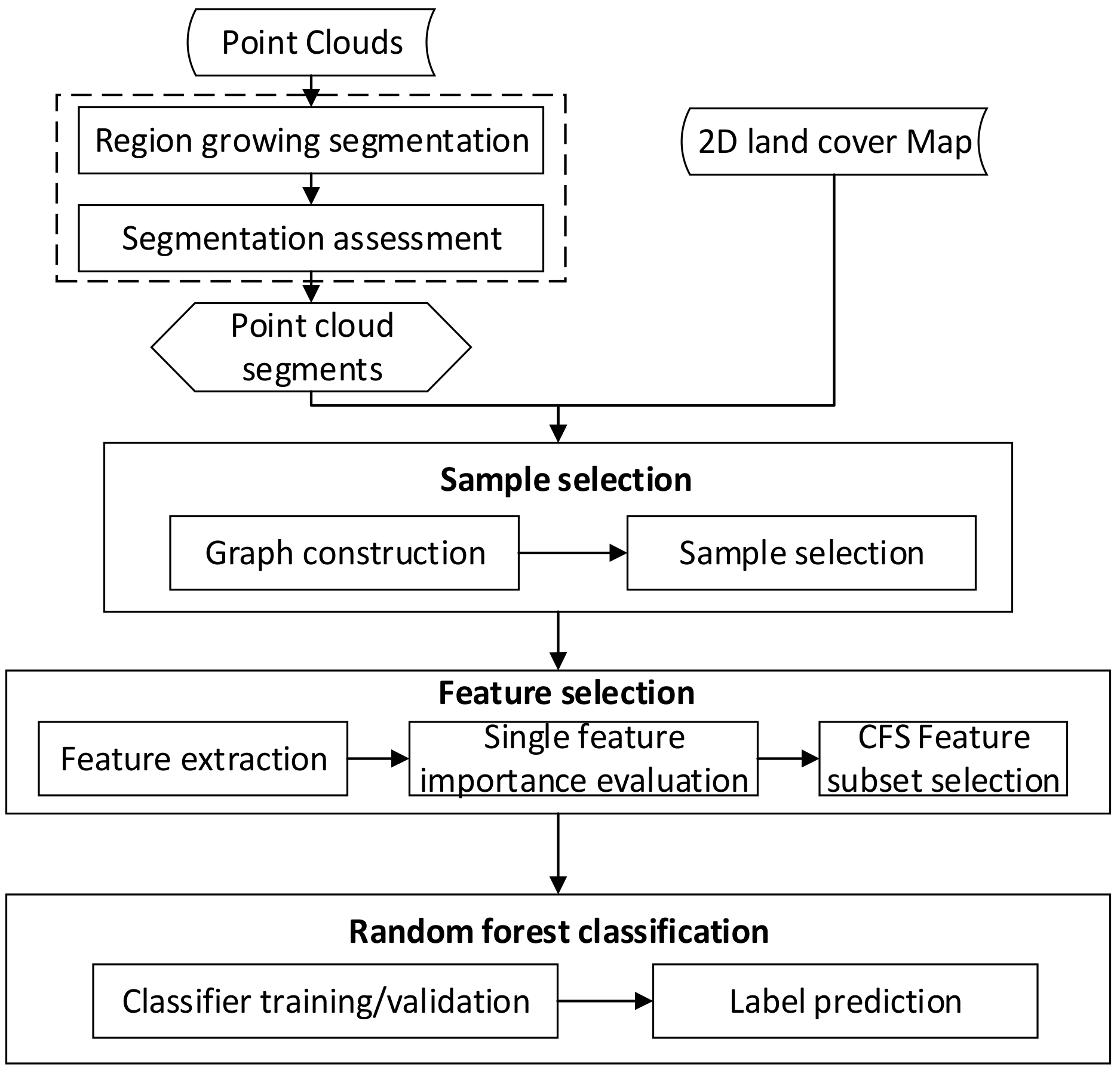
Figure 1 shows the workflow of the proposed method. It consists of four main steps, namely: (1) segmenting 3D point clouds through a region growing algorithm and assessing its quality; (2) automatically selecting samples from point segments with the aid of a 2D land cover map; (3) selecting an optimal feature set; and (4) classifying the point cloud segments with the selected samples and optimal feature set.
2.1. Segmentation of Point Clouds and Segmentation Assessment
For any segment-based approach, one important step is to determine the neighborhood parameter for identifying segments, as a result of its impact on the classification results. As suggested in Section 1, segmentation divides an input point cloud dataset into meaningful subsets. In the proposed approach, region growing segmentation [10,26,27] has been adopted.
2.1.1. Region Growing Segmentation
The region growing approach is a bottom-up technique that expands from selected seed points to neighboring points, and groups points deemed to be from the same surface patches. During the expansion process, a similarity index based on the chosen homogeneity criteria is computed. The process terminates when no additional neighboring points that meet the homogeneity criteria can be found. The success of this approach hinges on the choice of seed points, the homogeneity criteria, and the identification of the neighborhood [28].
To determine the seed regions, this study firstly calculates the curvature value of each point, and secondly, it sorts all of the points in the ascending order according to their curvature values. A seed list is subsequently built, with the first seed point being selected as the one with minimum curvature value. The seed list is maintained by adding the neighboring points of the current seed and removing the current seed. If the seed list is empty, a new seed point with a minimum curvature value of the remaining points is added. This process iterates until all of the points are segmented.
To determine the homogeneity criteria, the normal of each point is calculated by incorporating its neighboring points. A smoothness threshold is defined in terms of the angle between the current seed point and its neighboring points.
The identification of the neighborhood typically employs either the k-nearest-neighborhood (KNN) search [29] or the instance radius search [5]. The former is based on a fixed number of k neighboring points that approximates the density-adaptive search. The latter is based on a fixed search radius that corresponds to a fixed geometrical range. For the proposed approach in this study, the KNN search has been adopted, given that the TLS point cloud density tends to vary greatly according to the distance to the scanner and noises.
The number of nearest points, k, can be regarded as the neighborhood scale, which not only impacts segmentation, but also affects the feature extraction and classification in the later steps. The adaptive determination of a suitable scale of the analysis for each point cloud dataset is therefore warranted. A two-step method of finding an optimal scale is proposed in this study. In the first step, a series of segmentations with different k values are conducted. In the second step, the segmentation results are evaluated and compared. In the next sub-section, the method of assessing the segmentation results is elaborated.
2.1.2. Quality Assessment
Existing literature has suggested a number of quantitative metrics for assessing the segmentation outcomes [27,30], which can be either over- or under-segmentation. Over-segmentation refers to two neighboring segments belonging to the same surface that are separated. Quantitatively, it can be evaluated by a two-step process. The first step involves obtaining the surface roughness of a segment, as follows:
where is the number of points in a segment and is the normal distance of point to the best-fitted plane of the segment.
The second step used a pairwise comparison of the surface roughness values of the two neighboring segments. If the surface roughness values are equal to or lower than those of the constituent segments, the two segments are combined. The degree of over-segmentation is then calculated using the following equation:
where is the number of over-segmentation, and the number of the derived segments.
The measurement under-segmentation is made against the average surface roughness of all of the derived segments, defined as follows:
where is the average surface roughness, the number of points in the -th segment, and the surface roughness of the -th segment.
If the surface roughness value of a derived segment is significantly higher than the average surface roughness, it will be deemed under-segmentation. The degree of under-segmentation is calculated as follows:
where is the number of under-segmentation, and the total number of derived segments.
The OSeg and USeg, once obtained, are used to evaluate the segmentation quality under different scales (i.e., different k values). Smaller values of these measurements demonstrate a better segmentation quality. The optimal segmentation scale is obtained by comparing the metrics of the different segmentation results, which is used for further processing in the later steps.
2.2. Sample Selection
Following the segmentation is the selection of samples for training and testing purposes. In the proposed method, the automatic selection of samples is assisted by an existing 2D land cover map and by leveraging on the graph, , that captures the topological relationships between the segments.
2.2.1. Graph Construction
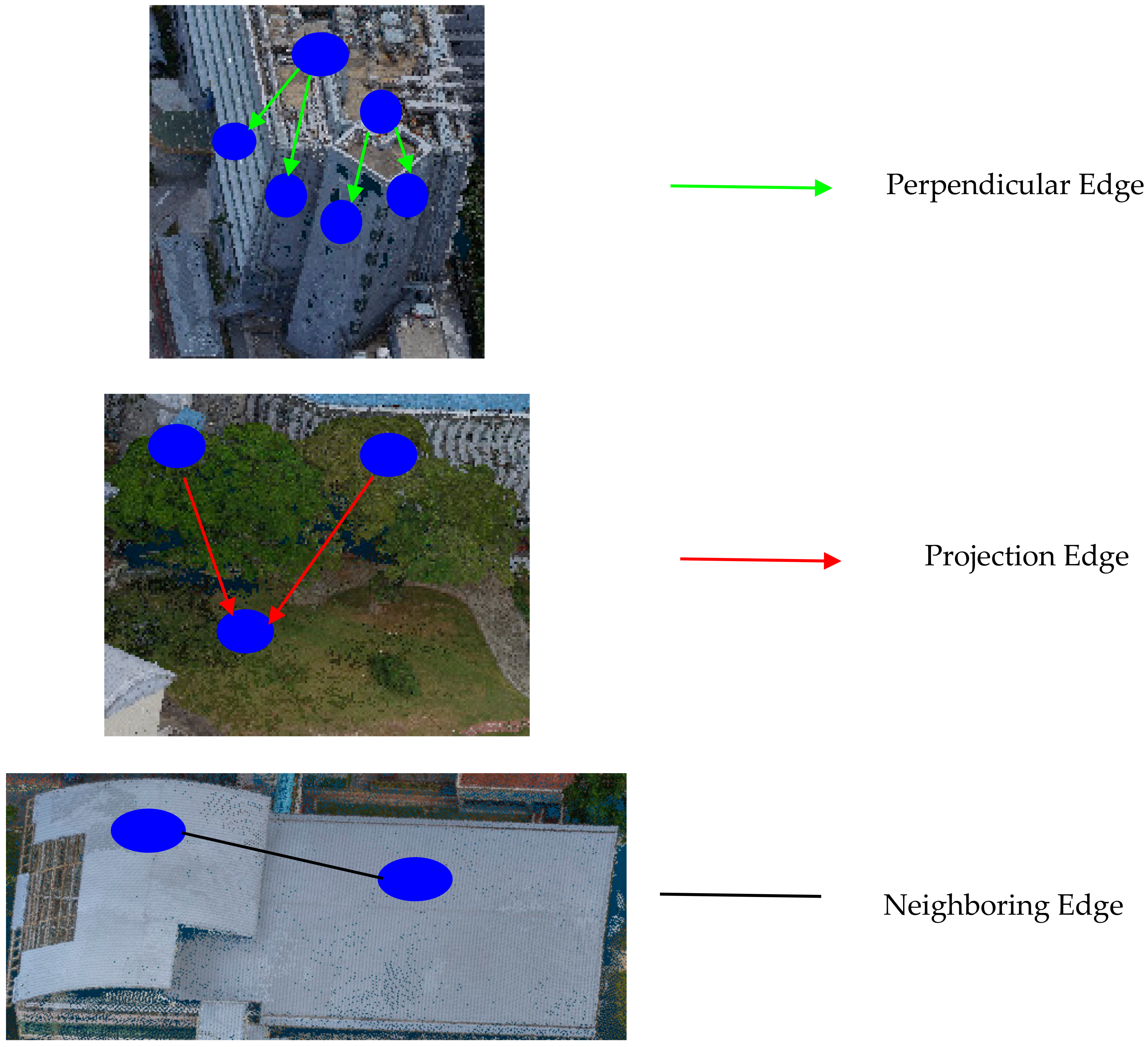
The construction of the graph, , where V is a set of nodes each of which represents a segment, and E is a set of edges each of which represents the topological relationships between two connected segments, is carried out by taking the derived segments as an input. In order to determine the type of topological relationship between two segments, the boundaries of each segment are first traced using the modified convex hull, suggested by Sampath and Shan [31], in order to generate a corresponding polygon. Once completed, all of the polygons are projected on to the XY plane. Every pair of polygons is checked if they are neighboring on an XY plane, and if they do, the proposed method further captures their topological relationship, which can be one of the following:
- Perpendicular relationship. If two polygons meet the two requirements, (a) the normal vectors of two polygon surfaces are nearly perpendicular and (b) one of the normal vectors is nearly parallel to the vertical (i.e., the angle between the two is negligible). If two nodes, and , hold the perpendicular relationship, they are connected by a directed edge, . The node with the higher average height value is designated as the starting node, while the node with the lower average height value is designated as the ending node. In practice, a roof and the walls underneath it usually hold this relationship.
- Projection relationship. If two polygons do not hold the perpendicular relationship but meet the following requirement: the extent of overlap between the two polygons on the XY plane is larger than a specified threshold . Two nodes that satisfy such a requirement are connected by a directed edge, . Similar to the perpendicular relationship, the node with a higher average height value is designated as the starting node, while the node with the lower average height value is designated as the ending node. Each edge in this topological relation is further assigned a weight value, which is obtained by calculating the height difference between the high and low average height values. In practice, the tree tops and the grassland, or the tree tops and the ground usually hold this relationship.
- Neighboring relationship. If two polygons do not hold one of the two former relationships, but are neighbors on the XY plane. The nodes representing the two polygons are connected by an undirected edge.
Figure 2 shows examples of the edges and the topological relations in the graph, , in which the blue circles represent the derived segments, and the lines with different colors represent three types of topological relationships.
2.2.2. Sample Selection with 2D Land Cover Map
After constructing the graph of the point cloud segments, the existing 2D land cover map from OpenStreetMap is employed to assist in the selection of samples, according to the following two criteria: (1) the degree a polygon is projected from a point cloud segment overlaps with the polygons in the 2D land cover map; and (2) the rules based on the topological relationships between different segments.
Obtaining the degrees of overlap for the first criteria is straightforward through using C++ and ArcGIS Engine. After the overlay operation, each projected polygon is assigned membership values to each of the land cover classes, which, in this study, are building, tree, grass, and ground, using the degree of overlap by Equation (5), as follows:
where is the -th segment, is a polygon in the 2D land cover map, is one of the classes in the 2D land cover map (, , , ), is the projection area of on XY plane, and is the size of the overlapping area of and on the XY plane.
Once the membership of a segment to each land cover class is obtained, the class with the highest membership value, hereafter termed the HM-class, is extracted. This step, however, does not imply that the segment is designated the HM-class because the classes to discern from the point cloud (i.e., roof, wall, tree, grass, and ground) and the classes in the 2D land cover map (i.e., building, tree, grass, and ground) do not hold one-to-one relations. In addition, the different dimensions of the land cover map and the point cloud (2D versus 3D) naturally lead to non-unique correspondences between z values and (x, y) values. For example, a segment with the largest membership to building might belong to roof or wall, and a segment with the largest membership to grass might belong to grass or tree. To handle such semantic mismatches, the graph, , that was previously constructed is used to refine the sample selection using the following rules and the search sequence starting from the class roof, and is followed by the class wall, tree, ground, and grass. Once a node is labeled with a meaningful class in the point cloud, it is excluded from the list of nodes being considered in the sample selection.
- (1)
- Roof. A node is considered to be representing a roof segment according to the following criteria. Firstly, its HM-class must be building and the membership value is above a certain value. Secondly, the normal vector of the segment is nearly vertical. Thirdly, the area of the projection of the segment on the XY plane is larger than a specified threshold, . The threshold is selected as there is hardly a roof with an area smaller than .
- (2)
- Wall. Once all of the roof segments are identified, the remaining nodes in graph are searched for wall segments by first identifying all of the nodes that are connected to the roof nodes through the edges of the designated perpendicular relationships. To handle potential noises, the angles between the normal vector of the identified nodes, and the horizontal are examined. If the angles are negligible, the segments represented by the corresponding nodes are considered to belong to the wall.
- (3)
- Tree. Two criteria are used to identify the tree nodes. Firstly, if the HM-class of the node in the remaining list of nodes is tree, it is identified as a candidate node. Secondly, for each candidate node, identify all of the connected projection edges, which can be outgoing projection edges, with the candidate node being the starting node or the incoming projection edges with the candidate node being the ending node, and calculate two values—the sum of the weights of all of the incoming projection edges and the sum of the weights of all of the outgoing projection edges. If the former is larger than the latter, the candidate node is labeled tree. The intuition behind this rule to exclude the ground and grass segments, which might overlap with tree on the XY plane but have relatively lower height values.
- (4)
- Ground. Two criteria are used to identify ground nodes. Firstly, if the HM-class of a node is ground, the node is identified as a candidate node. Secondly, similar to the second step for identifying tree nodes, identify all of the outgoing edges and the incoming edges and obtain the sums of the corresponding edge weights. If the sum of the weights for the incoming edges is smaller than that of the outgoing edges, the candidate node is labeled ground. The intuition of the two criteria is to exclude the possible tree segments above the ground.
- (5)
- Grass. The criteria to identify grass nodes are exactly the same as the criteria to identify ground, except that the HM-class of the candidate nodes for grass must be grass. The intuition is to exclude the possible tree segments above the grassland.
By using the above rules, samples of the classes in the input point cloud dataset are identified. One should note that only a part of the segments are identified as samples, and the labels of the remaining segments are unknown at the moment. In addition, setting the thresholds for this step of the proposed approach is not interpreted as introducing further human intervention. Rather, it reflects the flexibility of the proposed approach in allowing the specification of an ideal level of homogeneity for the selected samples.
2.3. Feature Extraction and Feature Selection
The features to describe the characteristics of 3D point cloud segments are generally of the following three types: eigen-based, spectral, and geometrical features. For the eigen-based type, eigenvalues , , and () are calculated for each segment, based on the covariance matrix. The eigenvector corresponding to the smallest eigenvalue () is known as the normal vector of the segment surface, and is represented as (, , ). Further measures can be calculated based on the eigenvalues, including th esum, omnivariance, eigenentropy, anisotropy, planarity, linearity, surface variation, and sphericity. For the spectral type, based on the red, green, and blue (RGB) values captured using TLS, six features in two sets of three are defined for each segment. The first three features are the mean red, mean green, and mean blue, which are defined as the mean values of all of the points within the segment on the three bands individually. The next three features are the red deviation, green deviation, and blue deviation, which are the standard deviation values of the three bands. For the geometrical type, four geometrical features are defined for each segment. The first is the number of points within a segment. The second is the projective area of the segment on its best-fitted surface plane. The third is the local point density within the segment, which is defined as follows:
where is the number of points within the segment and S is the projective area of the segment on its best-fitted surface plane.
The fourth geometrical feature is the average height, which is calculated as the average z-coordinate values of the points within the segment. A complete list of the features extracted can be found in Table 1.
To select the optimal feature set from the whole set of features, as defined, Weinmann et al. [8] suggested three types of quantitative evaluation methods (i.e., filter-, wrapper-, and embedded-based methods). The first type of method calculates the intrinsic properties of the training data to provide a score for each feature, and are insensitive to the classifier used. In contrast, the other two types of methods are classifier-dependent, and evaluate the performance of features during the process of training. In this study, the filter-based method is employed to avoid a classifier dependency.
There are many measures to assess the importance of a single feature. Among them, the gain ratio [32] has been proven to be a successful one. It is calculated as follows, and a higher gain ratio value indicates a higher importance of a feature.
where is a feature, and and are the gain value and split information of feature , which can be further referred to Quinlan [32].
Once the gain ratio values of all of the features are calculated, these features are sorted in descending order and then subject to the evaluation of their correlations using the best-first search (BFS) strategy and a Correlation-based Feature Selection (CFS) method [33]. The approach involves two steps. In the first step, the features are added to a feature set one by one, according to the descending order of their gain ratio values. In the second step, the feature set is evaluated by using the CFS metric, as follows:
where is the score of the feature set , is the number of features, is a class, is a feature, is the average relevance between the features and classes, and is the average relevance between the features and features.
A stopping criterion of adding new features is used to prevent the BFS search from exploring all of the possible combinations of features, and is set so that the CFS score does not increase when the feature set is added for five consecutive times. The above procedures are implemented in a non-commercial software Weka 3.8 (Waikato Environment for Knowledge Analysis). The optimal feature set is selected by using the above method, and are further used for classification in the next step.
2.4. Classification of Point Cloud Segments
Once the samples and optimal feature set have been selected, using the approach described in Section 2.2 and Section 2.3, they are used to classify the point cloud segments. Firstly, following Li et al. [34], the selected samples are divided randomly into two equal parts, one as the training set and the other as a test set. The training set and optimal feature set are used as inputs to train a classifier. In this study, the random forest (RF) classifier [35] is utilized for classification, given that it has been demonstrated effectively in 3D point cloud classification [17]. An RF classifier is an ensemble classifier based on a classification and regression tree (CART). It is composed of a number of decision trees that are trained independently, and the final classification results are determined by the majority vote of all of decision trees. A decision tree is constructed as follows:
- (1)
- Select, randomly from the training set, a sample set by bagging or bootstrap [36];
- (2)
- Select, randomly, a feature subset from the optimal feature set. The number of selected features in the feature subset approximates , where is the number of features in the optimal feature set;
- (3)
- Find the largest information gain for node splitting. A feature and its splitting threshold is determined at each node;
- (4)
- Iterate the splitting process until all of the samples in the same node have the same label or the decision tree reaches a maximum depth.
Another parameter required to train a RF classifier is the number of trees, which is set to a fixed number of 200 in order to achieve a reasonable classification accuracy within an acceptable duration. The adopted classifier is fully automated without any human intervention. Assume that the training sample set is and the test set is . Each training and test sample encapsulate a feature vector with dimensions, in which is the number of features in the optimal feature set. Each sample belongs to a class , where is the total number of labels ( in this study). The training set vector in a d-dimensional feature space is first employed to train the RF classifier. Then, the trained RF classifier is further employed to classify the test set, . The classification results are quantitatively evaluated by comparing the classified labels of the test samples with their actual labels.
3. Study Area and Datasets
The effectiveness of the proposed approach is tested using three datasets. The first two datasets, hereafter named Dataset1 and Dataset2, were collected by the Virtual National University of Singapore (NUS) project, while the third dataset, hereafter named Dataset3, is a publicly available and labeled 3D point cloud dataset of Oakland, Pennsylvania, created by Munoz et al. [37]. The characteristics of the three datasets and the purposes they serve in this study are described below.
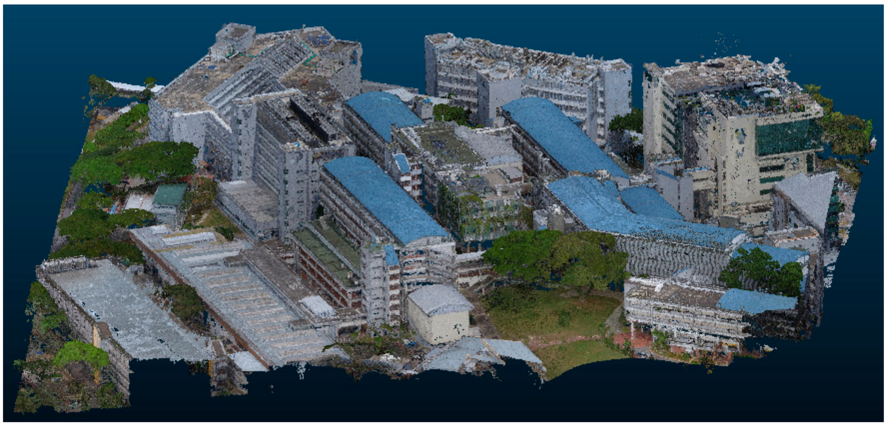
Dataset1 covers a smaller area of the NUS campus, which includes the computer center and a typical building of classrooms and offices on campus (Figure 3), while Dataset2 covers a larger area of the NUS campus, which includes the entire engineering school, with 21 main buildings and 5 lecture theaters (LTs) (Figure 4). Both areas are of similar characteristics, given that the buildings there were developed around the same time and were located in similar terrains. The former will be used to learn the details of the classification, while the latter will use the learned details to classify a larger study area. They are therefore used to demonstrate the effectiveness of the proposed approach in classifying point clouds of a typical university campus, and to demonstrate the transferability of the proposed method from a smaller to a larger dataset.
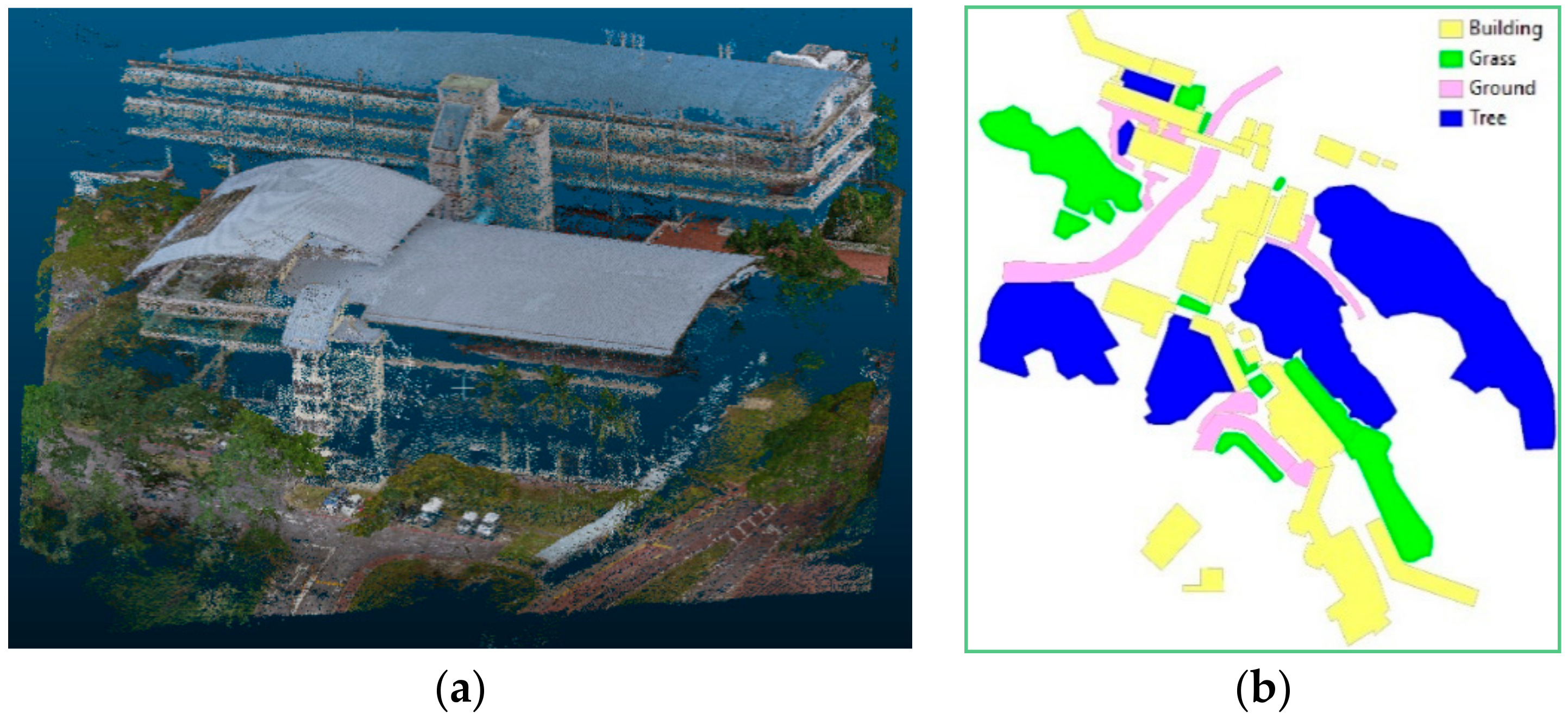
Both Dataset1 and Dataset2 contain LiDAR point clouds acquired by a terrestrial LiDAR scanner during the leaf-on season. Nicknamed the Garden City, Singapore is famous for greenery across the whole country. The NUS campus is no exception. As such, the two datasets exhibit high level of occlusions due to the presence of trees. In addition, the campus is situated on a terrain with internal relief of more than 60 m, which results in additional challenges to classify the LiDAR point clouds. The relief also allows placing the terrestrial LiDAR scanner on higher grounds so as to capture a more complete view of the study area, including the roofs of buildings. Aside from the LiDAR data, Dataset1 also includes a corresponding 2D land cover map from OpenStreetMap (www.openstreetmap.org), consisting of polygons of four land cover classes (i.e., building, tree, ground, and grass). The 2D land cover map was registered with the 3D point clouds to be used as ancillary data to assist in point cloud classification. Dataset1 and Dataset2 contain 1,263,253 and 14,452,784 points, respectively.
To demonstrate the feasibility and transferability of the proposed method to another area, this study also incorporates the Oakland 3D point cloud dataset [37] as a benchmark. This dataset, named Dataset3, includes four different scenes, one designated for training purposes (Figure 5), while the remaining three are designated for testing purposes (Section 4.6). The point cloud was acquired by an MLS with 44 classes, prototypical of an urban environment, such as utility pole, ground, facade, car, and garbage. In this study, some classes were merged and reassigned to other classes (e.g., points of ground, paved road, trail, and walkway were all labeled as ground). Some classes were removed (e.g., car, door, and window). All of the points were filtered and remapped from 44 to 4, with the following labels: wall, ground, tree, and grass, resulting in a total of 400,000 points.
4. Experiments and Analysis
4.1. Segmentation Results of Multiple Scales
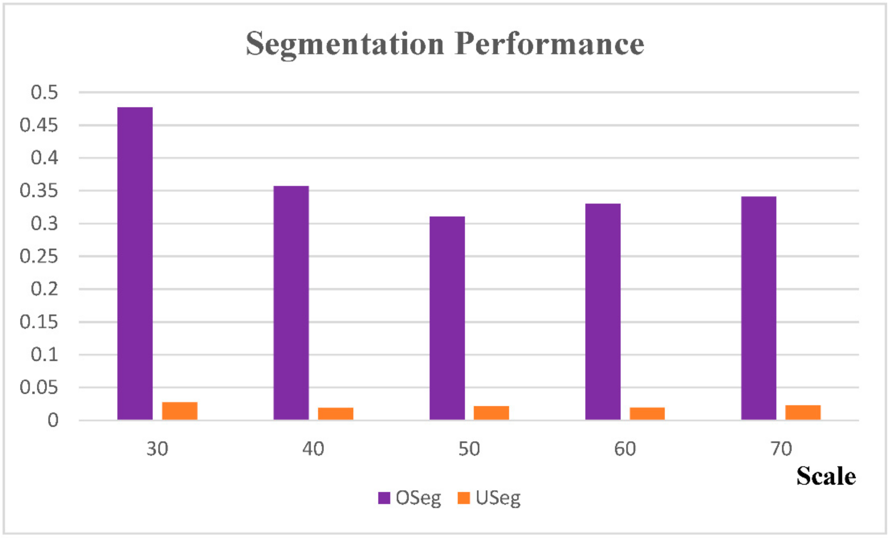
To find the optimal scale (the number of nearest points, k) for segmentation, a series of segmentation tests were conducted at different scales. In this study, five k values from 30 to 70, with an increment of 10, were used. The smoothness threshold was set as . After the region growing segmentation, each segmentation result was evaluated using OSeg and USeg (Figure 6).
The evaluation result suggests that the over- and under-segmentation are presented simultaneously at all scales. As the k increases, the OSeg first drops and then picks up after k >50. For the under-segmentation, the lowest USeg appears at k = 40. Considering both OSeg and USeg, the optimal scale, k, can be either 40 or 50. However, as the OSeg values are much higher than the USeg values, the OSeg carries a heavier weight for determining the optimal segmentation scale. In this study, the optimal scale, k, was therefore set to 50. The corresponding segmentation result of Dataset1 is shown in Figure 7. The proposed methods segmented 1,263,253 points into 1061 segments, thus reducing the computational resources needed for classification at the later stage. Note that not all of the points in the point cloud were included in the segment clusters, because we set a limit of the minimum number of 50 points within each segment. The remaining points were thus called rough points.
4.2. Results and Evaluations of Sample Selection
The segments derived in the previous step was then used to construct the graph, , for sample selection. The graph was constructed using all 1061 segments, and the relationships between the different segments were built and stored in the graph. After completing the graph, 2D land cover data in Dataset1 (Figure 3b) was employed to select samples from the graph. A total of 419 samples were chosen, including 15 roof segments, 107 wall segments, 21 ground segments, 259 tree segments, and 17 grass segments. A visual inspection found 15 incorrectly labeled samples (i.e., an overall precision of the sample selection of 96.42%). These samples represented different categories with various segment sizes, shapes, heights, data densities, and scanner positions. The selected samples were further used in the subsequent steps of the feature set selection and classification.
4.3. Results of Optimal Feature Set Selection
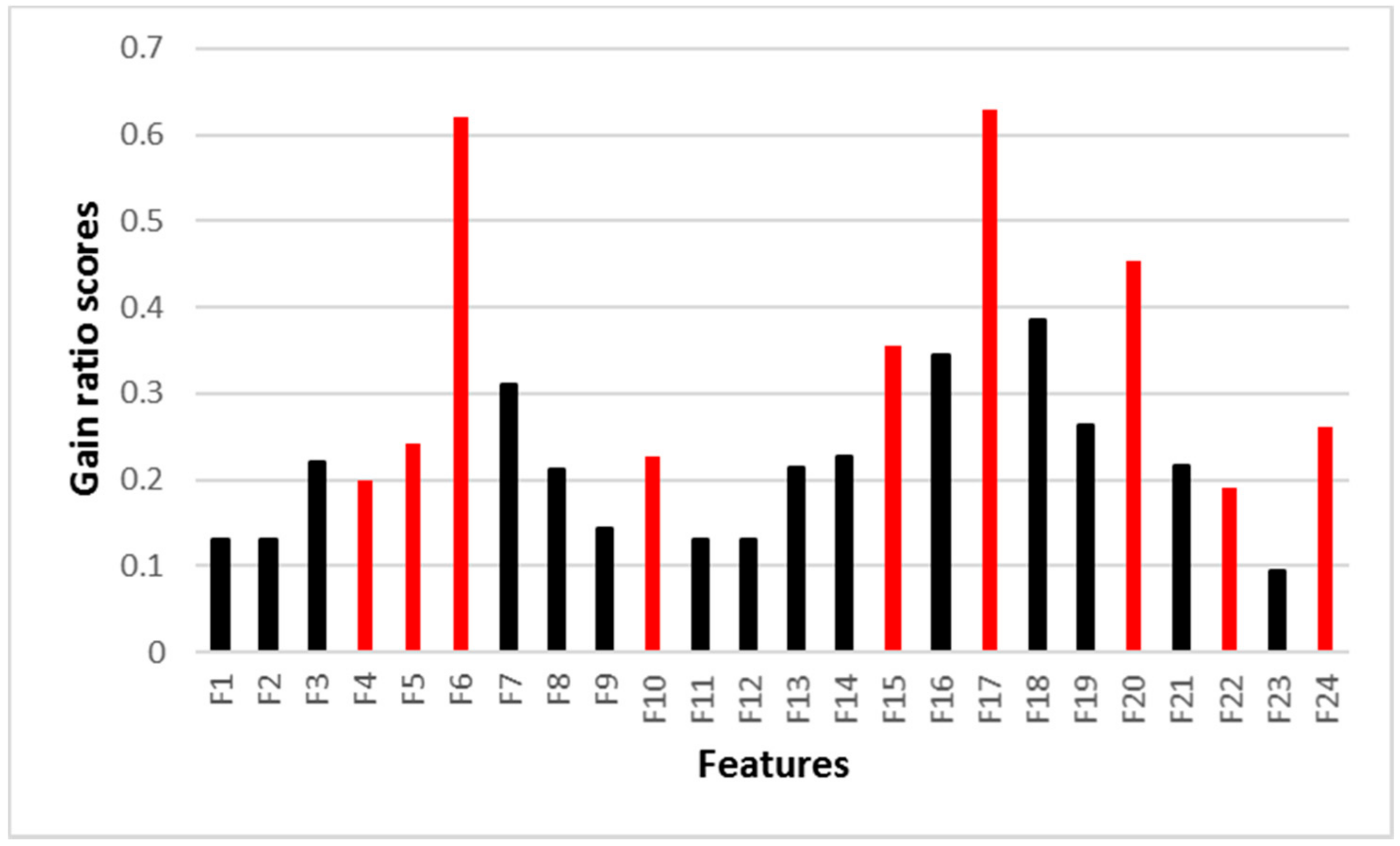
The selected samples were employed in the optimal feature set selection. Firstly, the importance of each single feature was evaluated using the gain ratio index. Overall, the result, which is shown in Figure 8, suggested that the spectral features (–) were more important than the eigen-based features (–) and geometrical features (–). A further examination of the result showed that the top five features with the largest gain ratio scores were , , , and (i.e., mean blue, normal_z, blue deviation, red deviation, and mean red). However, not all of the top ranked features were selected because of the relevance between them. In this study, the CFS method and BFS strategy were combined to select the optimal feature set, which considered the relevance between the features. The red bars in Figure 8 represent the features selected into the optimal feature set. The selected features of the CFS include , , , , , , , , , corresponding to normal_x, normal_y, normal_z, anisotropy, mean red, mean blue, blue deviation, local point density, and average height. Among these nine features, four (i.e., , , , and ) are eigen-based features, three (i.e., , , and ) are spectral features, and two ( and ) are geometrical features. The results suggested that (1) the normal vector plays an important role in point classification, especially its value at z direction (i.e., normal_z); (2) despite the fact that some of the spectral features (, , and ) have a high contribution, because of the correlation with other spectral features (the correlation coefficients between mean green and mean red, red deviation and blue deviation, and green deviation and blue deviation are 0.964, 0.950, and 0.965, respectively), they should be avoided; (3) although the geometrical features do not have very high gain ratio scores, they are still selected into the optimal feature set because of the low correlations (less than 0.1) with other two types of features.
4.4. Classification Result of Dataset1
After choosing the samples and features, the training sample set and optimal feature set were used to train an RF classifier. The trained RF classifier was further used to classify the point segments in Dataset1. Each segment in Dataset1 is typed either as a (1) training segment; (2) test segment; or (3) unlabeled segment. All of the segments were reclassified by the trained RF classifier, in which both the training segments and the test segments were used for accuracy assessment. The selected samples were divided into training and test segments, following the standard approach for evaluating the performance of a classifier. A total of three metrics were employed to evaluate the classification performance. The first two are precision and recall [38], in which precision is also known as a producer’s accuracy, and recall is also known as a user’s accuracy. The third metric is F-score, which integrates precision and recall into one measure, as follows:
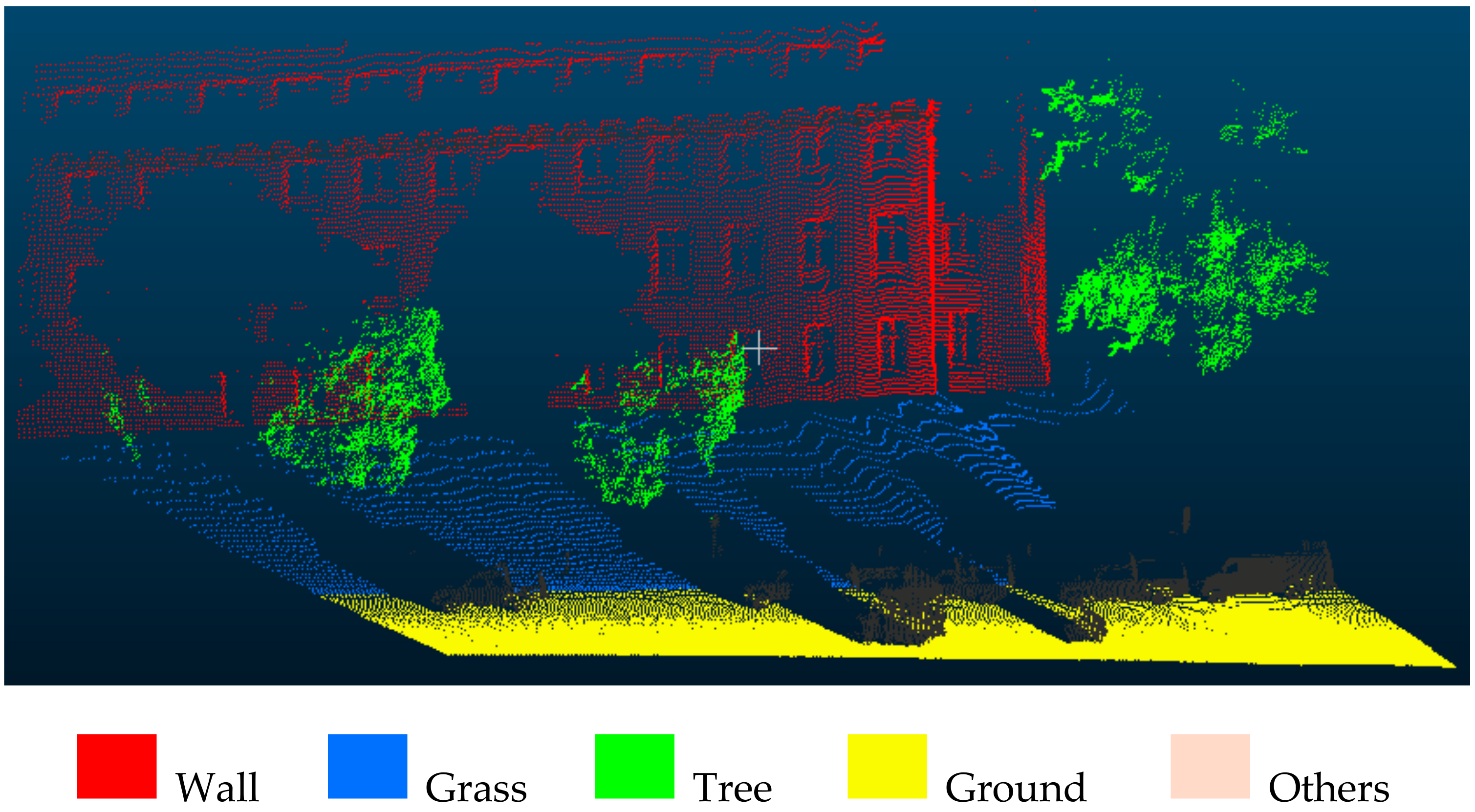
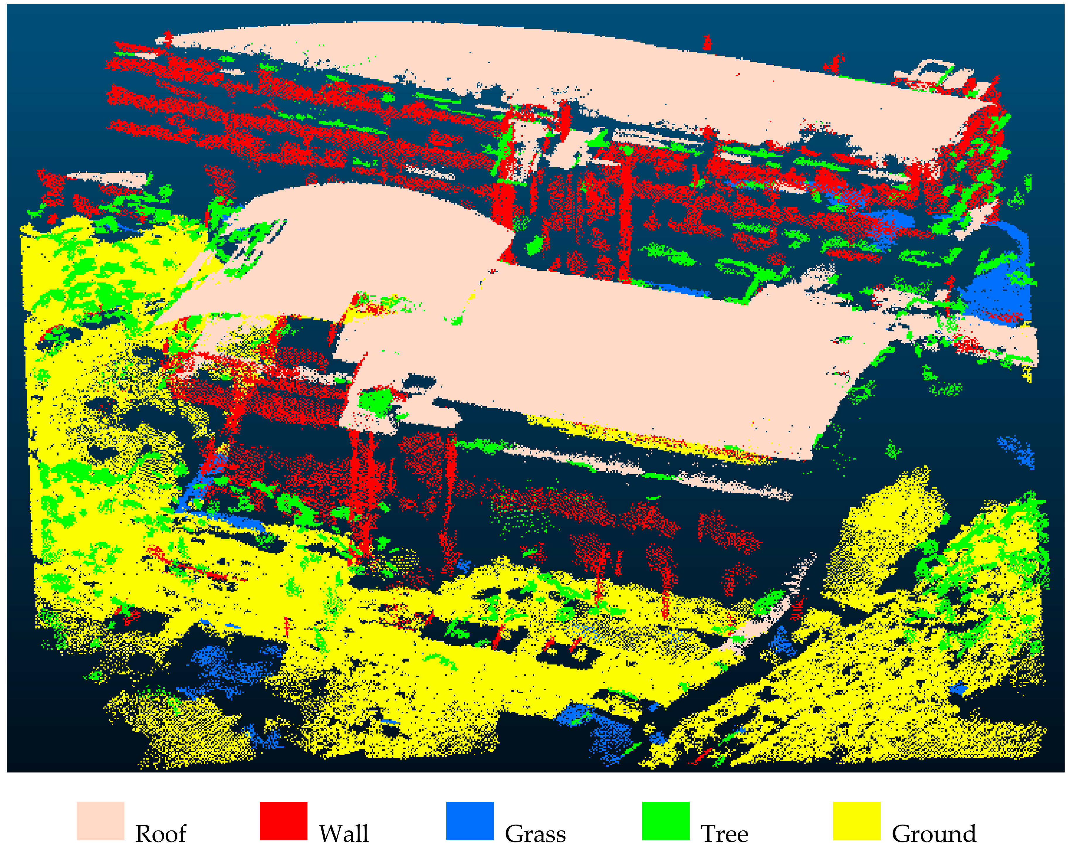
Figure 9 shows the classification results of the point clouds in Dataset1. The proposed approach correctly recognized the classes for most points, with an overall accuracy of 94.07% on the test set (Table 2). The highest F-score was obtained for the ground class (99.45%). The second highest F-score was obtained for the wall class, with a precision and recall both above 95%. The lowest F-score obtained was the grass class, with a precision of 62.70%. Through visual inspection, such low precision was mainly caused by the misclassification of points belonging to grass into tree. One might argue that these two classes can be easily distinguished using height. While generally true, this is not the case for our study site, which sits on an internal relief of over 60 m. Overall, the classification results of Dataset1 were satisfactory.
4.5. Classification Result of Dataset2
While the proposed method performed well for a small point cloud of Dataset1, this section illustrates that the details learned from a particular dataset by the proposed method are transferable to a larger dataset. Being able to do so is important for a large site classification, because the resources needed to train a smaller dataset are significantly less than that for a larger dataset. In this study, we used the learned the parameters and the trained classifier from the first experiment to classify the point clouds in Dataset2 (Figure 4), which shares similar characteristics with Dataset1. To do so, the point clouds in Dataset2 were first segmented with the optimal scale learned from Dataset1 (i.e., k = 50), and secondly, for each segment, nine features in the optimal feature set, described in Section 4.3, were extracted. Thirdly, the trained classifier by Dataset1 was used to classify point segments of Dataset2.
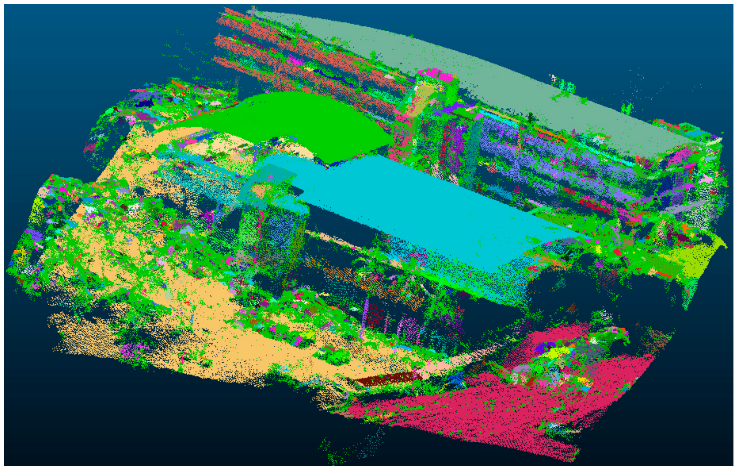
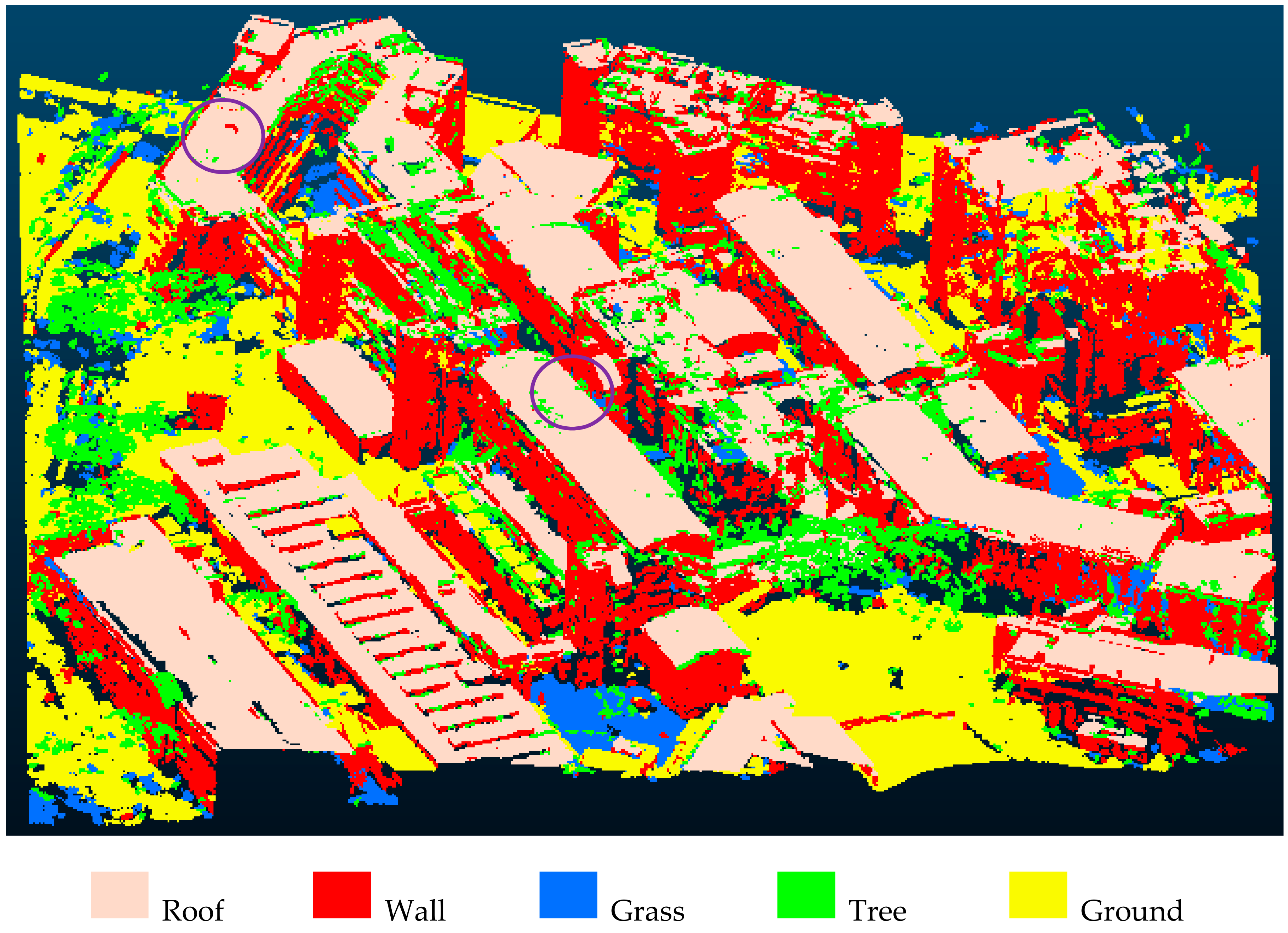
Figure 10 presents the result of the classification, which again consists of five classes, roof, wall, grass, tree, and ground. A total of 11,584 segments were obtained. In order to assess the classification quality of Dataset2, 10% (1200) of the segments were randomly selected and visually inspected.
Table 3 presents the quantitative assessment of classifying Dataset2. The highest precision is obtained for the class wall (97.99%). The reason for such high precision is straightforward; walls are usually vertical and thus it is highly unlikely to classify wall segments into other classes. The highest recall (92.61%) and F-score (93.70%) were both obtained for the class ground, indicating that ground is easily recognizable. Following the first two classes is the class roof (F-score of 89.44%). Figure 10 shows that a small portion of roof points are misclassified as tree (in purple circles). Such misclassification is likely to be the result of the following. Firstly, the study area is located in a heavily vegetated area where roofs are often occluded as a result of the presence of trees. Secondly, the roof and tree are both above the ground and have similar height attributes, thus causing confusions during classification. The grass and tree classes have the lowest (79.06%) and second lowest (86.19%) F-score. There were still significant confusions between these two classes, owing to their similar spectral features.
Compared to the quantitative classification results of Dataset1 (Table 2), the F-scores of roof and grass in Dataset2 are higher than those in Dataset1, while the F-scores of wall, tree, and ground are slightly lower than those in Dataset1. The overall accuracy of classification results on Dataset2 is 91.13%, which is similar to the overall accuracy of 94.07% for Dataset1. It can be concluded that the transition of the learned knowledge from Dataset1 to Dataset2 was satisfactory, suggesting that the proposed method is generalizable for larger areas with similar building and vegetation configurations and reliefs.
4.6. Classification Result of Dataset3
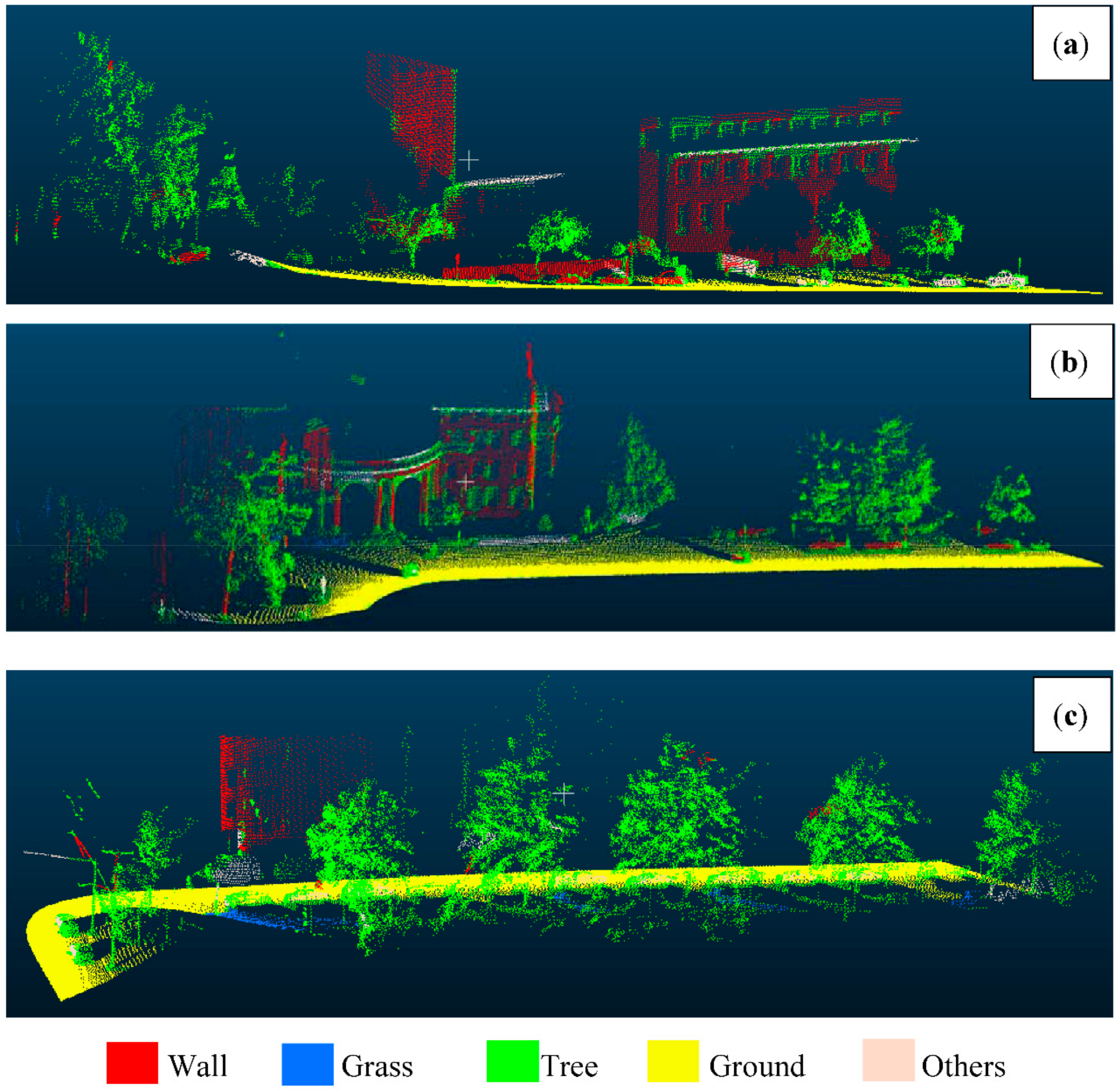
This section presents the result of classifying the point clouds with the different characteristics represented by the Oakland Point Cloud Dataset. A procedure similar to that used to classify Dataset1 was employed. The only difference is that for Dataset3, the training and test samples have already been provided. Firstly, the neighborhood scale was learned, which turned out to also be 50. The neighborhood scale is then used to segment Dataset3. Secondly, the full feature set in Table 1, except the spectral features, were extracted for each segment. The optimal feature set was selected and included six features, namely, normal_x, normal_y, normal_z, anisotropy, local point density, and average height. Again, the random forest classifier was used for both training and testing. The classification results of Dataset3 are shown in Figure 11. In addition, a separate experiment was carried out with an identical setup, except that the full feature set was employed.
Table 4 presents the results with the optimal feature set and the full feature set. While both sets achieved a high overall accuracy, the optimal feature set edging the full feature set by about 1.2%. The former also achieved a better performance for individual classes, as can be observed from the evaluation metrics (precision, recall, and F-score) of the individual classes in Table 4. As to the classification results of Dataset3 with the optimal feature set, it was observed that the recall of the wall (85.02%) and the precision of the tree (82.15%) were not very high. This was caused by the mixture of the tree and wall points, which can also be validated from the visual results of Figure 11. Some of the wall points were wrongly classified as tree (Figure 11a,b). The reasons for such lower-than-expected performance may be that (1) no color features were involved in this dataset and (2) the training samples in Figure 5 did not capture sufficient characteristics of walls and trees. To improve the results, more samples should be incorporated.
In addition, we compared our result with the results of (1) the non-associative higher-order Markov model (NAHO MRF) by Najafi et al. [39]; and (2) the method by Weinmann et al. [8]. Tge NAHO MRF adopted a set of non-associative context patterns to describe the higher-order geometric relationships between the different class labels. Weinmann et al. [8] used different scales, different feature sets, and different classifiers in order to obtain a number of classification results, and we chose the one with the highest overall accuracy. Note that the classification accuracies of the two methods were acquired from Najafi et al. [39] and Weinmann et al. [8], separately (Table 4).
Although all of the methods adopted the same dataset (i.e., the Oakland dataset), different classes were chosen for the experiments. Weinmann et al. [8] did not differentiate grass and ground, but considered them as one class (i.e., ground, but they incorporated two additional classes, that is, wire and pole). Compared to the classes considered in this study, Najafi et al. [39] incorporated an additional vehicle class. The comparison between the results of the three studies showed that our approach achieved the highest precision for wall (94.74%) and the highest F-score for ground (100%), and the overall accuracy of our approach was 4.81% higher than that of the method by Weinmann et al. [8] (Table 4). The better performance of our approach is likely to be explained by the following reasons: (1) the different classes adopted in different methods and (2) a segment-based approach was adopted rather than a point-based approach in other two studies. In order to analyze the impact of the point- and segment-based approaches to the classification results, we further compared these two methods in the next section.
4.7. Comparison of Segment-Based and Point-Based Classification Results
Segment- and point-based methods have both been employed in previous point cloud classification studies [2,11]. It is well known that the segment-based methods are more efficient. It is less certain, however, regarding how both methods perform in terms of classification accuracy. A comparison of the performance of the classification by these two methods is therefore provided.
The experiment of the point-based classification is conducted on Dataset1. In order to ensure a fair comparison, we adopted the same sample set for training and testing. The only difference was that the samples used were points, thus the features were also extracted and calculated based on points. As some features in Table 1 are selected to describe the characteristics of segments, that is, the standard deviations of R, G, and B band (,); number of points (); area (); and local point density (), they were excluded for this comparison. In terms of an optimal feature set, the proposed feature selection method was employed. The RF classifier was first trained by the training set and then further used to classify the test set for its accuracy assessment, as well as the whole point cloud of Dataset1.
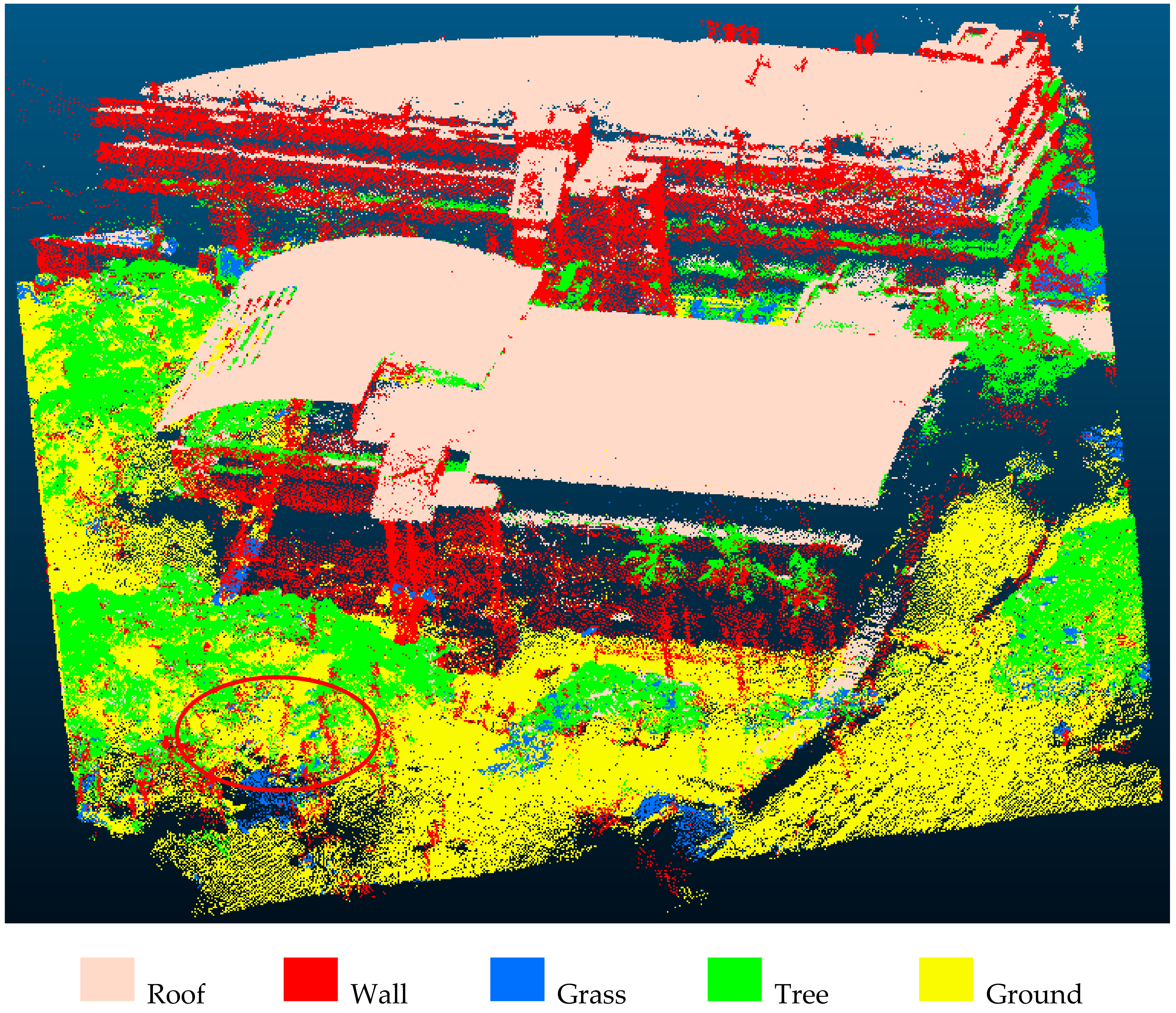
Figure 12 shows the point-based classification result. Compared with the segment-based classification result in Figure 9, the results produced by the point-based classification are more fragmentized, exhibiting the salt and pepper effect described by Blaschke et al. [40] in their effort to perform per-pixel classification of 2D images. In Figure 12, some points of trees and ground (the red circle) were misclassified into wall. One possible account for such error was that the classifier tends to label the points with horizontal normal as wall, according to the learned details. These kind of errors can be significantly reduced when these points are clustered into segments.
Comparing the evaluation result of the point-based classification and the segment-based classification using the test set showed that the overall accuracy of the latter (94.07%, Table 2) is higher than that of the former (89.41%, Table 5), with an improvement of 4.66%. An improvement of around 5% can already be regarded as a significant change, according to Janecek and Gansterer [41]. More importantly, the overall error rate (1-overall accuracy) is decreased by nearly half for the segment-based classification. For the individual classes, segment-based classification produced a significant higher F-score for wall, grass, tree, and ground, while the F-score of roof by the two methods were nearly the same. Such outcomes are possibly explained by (1) the segment-based methods that were able to generate more features, of which some were extremely useful for classification; and (2) the segment-based method involving more local contextual information and at the same time reducing the heterogeneity of the point features.
4.8. Computational Performance
A prototype based on C++ was developed for the proposed method. The Point Cloud Library (PCL) was used for the loading and segmentation of point clouds. The procedures of the feature selection and random forest classification were performed by the non-commercial software of Weka. All of the experiments were performed on a desktop computer with a CPU Intel Core i7-6700 processor, with 3.4 GHz and 32-GB RAM. One of the main computational hurdles of the proposed method lies in the segmentation procedure with a computational complexity of . In practice, for the point cloud of Dataset2 with 18,458,049 points, the elapsed time for one segmentation is nearly 18.5 min. Although the segmentation procedure takes some time, the number of elements (14,444) for the segment-based classification is greatly reduced compared with that of the point-based method (18,458,049); therefore, the computation time and load were significantly reduced.
5. Conclusions
This study presents a segment-based approach to classify the point cloud, an important step to facilitate the construction of semantic 3D models. The approach innovates by first selecting labelled samples through fusing TLS data and 2D land cover maps, and secondly, by automating the learning of parameters, including the optimal scales and features. It involves four successive steps, namely, (1) point cloud segmentation; (2) optimal sample selection; (3) optimal feature set selection; and (4) point cloud classification. Land cover maps played an important role in the automatic selection of a number of the representative samples, which were used in the later steps of selecting the features and training the classifier. Three datasets were used to validate the effectiveness of the proposed approach, in terms of its accuracy and transferability. The first dataset, termed Dataset1, covers a small area of the NUS campus. It consists of two buildings. The second dataset, termed Dataset2, covers a much larger area of the NUS campus. It consists of 21 main buildings and 5 lecture theatres. The third dataset, termed Dataset3, is a labeled on the point cloud dataset of Oakland, Pennsylvania. It consists of typical objects found in an urban environment.
Through executing the four successive steps in the proposed approach, using the three datasets, this study demonstrated the effectiveness of leveraging the surface roughness as a measure to automatically determine the neighborhood scale for achieving the best segmentation performance. The use of 2D land cover maps is proven to be advantageous in automating the selection of the samples for training and testing purposes; the samples selected are unbiased and with an accuracy higher than 96%. The optimal feature set was selected using the best-first search, and the correlation-based feature selection is shown to obtain a higher overall accuracy than using the full feature sets. The experiments performed on Dataset1, Dataset2, and Dataset3 showed the transferability of the proposed approach from a smaller to a larger dataset, and between two sites that exhibit different characteristics. A further comparison between the segment- and point-based approaches was carried out using Dataset1. The result suggests that the former approach is indeed more advantageous than the latter approach. In summary, the proposed 3D TLS point cloud classification method makes the following two contributions: (1) a method of fusing the 2D land cover maps and 3D LiDAR points is proposed for inferring point labels and selecting samples; and (2) a formalized procedure to automate the selection of the parameters for 3D point cloud classification is implemented with the aid of 2D land cover maps.
This research has two immediate applications. Firstly, the proposed method can be used to classify point clouds covering a larger area by using a small area as the training set. Such a finding is important for scaling up the point cloud operations in urbanized areas, where the urban configurations are often similar and repetitive. Secondly, the classification results of the labeling points can be used as a benchmark dataset for further academic research. For future work, we plan to examine the sensitivity of different land cover maps, and thus different land cover categories, on the classification results. We also plan to explore the automatic modeling of 3D scenes based on the labeling points, which may involve object boundary tracking and boundary regularization, as the method presented here provides one prerequisite to achieve the stated goal.
Author Contributions
Conceptualization, C.-C.F. and Z.G.; Methodology, C.-C.F. and Z.G.; Software, Z.G.; Validation, Z.G.; Formal Analysis, Z.G.; Investigation, Z.G.; Resources, Z.G.; Data Curation, Z.G.; Writing-Original Draft Preparation, C.-C.F. and Z.G.; Writing-Review & Editing, C.-C.F. and Z.G.; Visualization, Z.G.; Supervision, C.-C.F.; Project Administration, C.-C.F.; Funding Acquisition, C.-C.F.
Funding
This research was part of the Virtual National University of Singapore (VNUS) project funded by NUS under grant number WBS R-705-000-035-133.
Acknowledgments
We want to thank all the VNUS team members for providing the NUS dataset used in this paper.
Conflicts of Interest
The authors declare no conflict of interest.
References
- Alexander, C.; Tansey, K.; Kaduk, J.; Holland, D.; Tate, N. An approach to classification of airborne laser scanning point cloud data in an urban environment. Int. J. Remote Sens. 2011, 32, 9151–9169. [Google Scholar]
- Niemeyer, J.; Rottensteiner, F.; Soergel, U. Conditional random fields for lidar point cloud classification in complex urban areas. ISPRS Ann. Photogramm. Remote Sens. Spat. Inf. Sci. 2012, 1, 263–268. [Google Scholar] [CrossRef]
- Kwak, E.; Habib, A. Automatic representation and reconstruction of DBM from LiDAR data using recursive minimum bounding rectangle. ISPRS J. Photogramm. Remote Sens. 2014, 93, 171–191. [Google Scholar] [CrossRef]
- Dorninger, P.; Pfeifer, N. A comprehensive automated 3D approach for building extraction, reconstruction, and regularization from airborne laser scanning point clouds. Sensors 2008, 8, 7323–7343. [Google Scholar] [CrossRef] [PubMed]
- Brodu, N.; Lague, D. 3D terrestrial lidar data classification of complex natural scenes using a multi-scale dimensionality criterion: Applications in geomorphology. ISPRS J. Photogramm. Remote Sens. 2012, 68, 121–134. [Google Scholar] [CrossRef] [Green Version]
- Lin, C.; Chen, J.; Su, P.; Chen, C. Eigen-feature analysis of weighted covariance matrices for LiDAR point cloud classification. ISPRS J. Photogramm. Remote Sens. 2014, 94, 70–79. [Google Scholar] [CrossRef]
- Wang, Z.; Zhang, L.; Fang, T.; Tong, X.; Qu, H.; Xiao, Z.; Li, F.; Chen, D. A multiscale and hierarchical features extraction method for terrestrial laser scanning point cloud classification. IEEE Trans. Geosci. Remote Sens. 2015, 53, 2409–2425. [Google Scholar] [CrossRef]
- Weinmann, M.; Jutzi, B.; Hinz, S.; Mallet, C. Semantic point cloud interpretation based on optimal neighborhoods, relevant features and efficient classifiers. ISPRS J. Photogramm. Remote Sens. 2015, 105, 286–304. [Google Scholar] [CrossRef]
- Richter, C.; Behrens, M.; Dollner, J. Object class segmentation of massive 3D point clouds of urban areas using point cloud topology. Int. J. Remote Sens. 2013, 34, 8408–8424. [Google Scholar] [CrossRef]
- Vosselman, G.; Gorte, B.; Sithole, G.; Rabbani, T. Recognising structure in laser scanner point clouds. Int. Arch. Photogramm. Remote Sens. Spat. Inf. Sci. 2004, 46, 33–38. [Google Scholar]
- Aijazi, A.; Checchin, P.; Trassoudaine, L. Segmentation based classification of 3D urban point clouds: A super-voxel based approach with evaluation. Remote Sens. 2013, 5, 1624–1650. [Google Scholar] [CrossRef]
- Yang, B.; Dong, Z. A shape-based segmentation method for mobile laser scanning point clouds. ISPRS J. Photogramm. Remote Sens. 2013, 81, 19–30. [Google Scholar] [CrossRef]
- Liu, K.; Boehm, J. A new framework for interactive segmentation of point clouds. Int. Arch. Photogramm. Remote Sens. Spat. Inf. Sci. 2014, 40, 357–361. [Google Scholar] [CrossRef]
- Awrangjeb, M. Using point cloud data to identify, trace, and regularize the outlines of buildings. Int. J. Remote Sens. 2016, 37, 551–579. [Google Scholar] [CrossRef] [Green Version]
- Zhu, Q.; Li, Y.; Hu, H.; Wu, B. Robust point cloud classification based on multi-level semantic relationships for urban scenes. ISPRS J. Photogramm. Remote Sens. 2017, 129, 86–102. [Google Scholar] [CrossRef]
- Lodha, S.; Fitzpatrick, D.; Helmbold, D. Aerial lidar data classification using Adaboost. In Proceedings of the IEEE International Conference on 3-D Digital Imaging and Modelling, Montreal, QC, Canada, 21–23 August 2007; pp. 435–442. [Google Scholar]
- Chehata, N.; Guo, L.; Mallet, C. Airborne lidar feature selection for urban classification using random forests. Int. Arch. Photogramm. Remote Sens. Spat. Inf. Sci. 2009, 38, 207–212. [Google Scholar]
- Mahmoudi, M.; Sapiro, G. Three-dimensional point cloud recognition via distributions of geometric distances. Graph. Model. 2009, 71, 22–31. [Google Scholar] [CrossRef] [Green Version]
- Qi, C.; Su, H.; Mo, K.; Guibas, L. PointNet: Deep learning on point sets for 3d classification and segmentation. In Proceedings of the 2017 IEEE Conference on Computer Vision and Pattern Recognition, Honolulu, HI, USA, 21–26 July 2017; IEEE: Piscataway, NJ, USA, 2017; Volume 1, pp. 652–660. [Google Scholar]
- Qi, C.; Yi, L.; Su, H.; Guibas, L. Pointnet++: Deep hierarchical feature learning on point sets in a metric space. In Advances in Neural Information Processing Systems; MIT: Cambridge, MA, USA, 2017; pp. 2099–5108. [Google Scholar]
- Zhao, R.; Pang, M.; Wang, J. Classifying airborne LiDAR point clouds via deep features learned by a multi-scale convolutional neural network. Int. J. Geogr. Inf. Sci. 2018, 32, 960–979. [Google Scholar] [CrossRef]
- Khoshelham, K.; Oude Elberink, S. Role of dimensionality reduction in segment-based classification of damaged building roofs in airborne laser scanning data. In Proceedings of the International Conference on Geographic Object Based Image Analysis, Rio de Janeiro, Brazil, 7–9 May 2012; pp. 7–9. [Google Scholar]
- Duda, R.O.; Hart, P.E.; Stock, D.G. Pattern Classification, 2nd ed.; Wiley: New York, NY, USA, 2001. [Google Scholar]
- Bouziani, M.; Goita, K.; He, D. Rule-based classification of a very high resolution image in an urban environment using multispectral segmentation guided by cartographic data. IEEE Trans. Geosci. Remote Sens. 2010, 8, 3198–3211. [Google Scholar] [CrossRef]
- Ma, L.; Cheng, L.; Li, M.; Ma, X. Training set size, scale, and features in Geographic object-based image analysis of very high resolution unmanned aerial vehicle imagery. ISPRS J. Photogramm. Remote Sens. 2015, 102, 14–27. [Google Scholar] [CrossRef]
- Sithole, G.; Vosselman, G. Automatic structure detection in a point cloud of an urban landscape. In Proceedings of the 2nd GRSS/ISPRS Joint Workshop on Remote Sensing and Data Fusion over Urban Areas: URBAN 2003, Berlin, Germany, 22–23 May 2003; pp. 67–71. [Google Scholar]
- Habib, A.; Lin, Y. Multi-class simultaneous adaptive segmentation and quality control of point cloud data. Remote Sens. 2016, 8, 104–126. [Google Scholar]
- Rabbani, T.; Van Den Heuvel, F.A.; Vosselman, G. Segmentation of point clouds using smoothness constraint. Int. Arch. Photogramm. Remote Sens. Spat. Inf. Sci. 2006, 36, 248–253. [Google Scholar]
- Hackel, T.; Wegner, J.; Schindler, K. Fast semantic segmentation of 3D point clouds with strongly varying density. ISPRS Ann. Photogramm. Remote Sens. Spat. Inf. Sci. 2016, 3, 177–184. [Google Scholar] [CrossRef]
- Lari, Z.; Habib, A. New approaches for estimating the local point density and its impact on Lidar data segmentation. Photogramm. Eng. Remote Sens. 2013, 79, 195–207. [Google Scholar] [CrossRef]
- Sampath, A.; Shan, J. Building boundary tracing and regularization from airborne LiDAR point clouds. Photogramm. Eng. Remote Sens. 2007, 73, 805–812. [Google Scholar] [CrossRef]
- Quinlan, J.R. Improved use of continuous attributes in C4. 5. J. Artif. Intell. Res. 1996, 4, 77–90. [Google Scholar] [CrossRef]
- Hall, M.A.; Holmes, G. Benchmarking attribute selection techniques for discrete class data mining. IEEE Trans. Geosci. Remote Sens. 2003, 15, 1437–1447. [Google Scholar] [CrossRef] [Green Version]
- Li, C.; Dong, X.; Zhang, Q. Multi-scale object-oriented building extraction method of Tai’an city from high resolution image. In Proceedings of the IEEE 3rd International Workshop on Earth Observation and Remote Sensing Applications, Changsha, China, 11–14 June 2014; pp. 91–95. [Google Scholar]
- Breiman, L. Random forests. In Machine Learning; Schapire, R.E., Ed.; Springer: Berlin, Germany, 2001; pp. 5–32. [Google Scholar]
- Efron, B. Bootstrap method: Another look at the jackknife. Ann. Stat. 1979, 7, 1–26. [Google Scholar]
- Munoz, D.; Bagnell, J.; Vandapel, N.; Hebert, M. Contextual classification with functional max-margon Markov networks. In Proceedings of the IEEE Conference on Computer Vision and Pattern Recognition, Miami, FL, USA, 20–25 June 2009; pp. 975–982. [Google Scholar]
- Guo, Z.; Du, S.; Li, M.; Zhao, W. Exploring GIS knowledge to improve building extraction and change detection from VHR imagery in urban areas. Int. J. Image Data Fusion 2015, 7, 42–62. [Google Scholar] [CrossRef]
- Najafi, M.; Namin, S.; Salzmann, M.; Petersson, L. Non-associative higher-order Markov networks for point cloud classification. In Proceedings of the European Conference on Computer Vision, Zurich, Switzerland, 6–12 September 2014; Springer: Cham, Switzerland, 2014; pp. 500–515. [Google Scholar]
- Blaschke, T.; Lang, S.; Lorup, E.; Strobl, J.; Zeil, P. Object-oriented image processing in an integrated GIS/remote sensing environment and perspectives for environmental applications. In Environmental Information for Planning, Politics and the Public; Cremers, A., Greve, K., Eds.; Metropolis Verlag: Marburg, Germany, 2000; Volume 2, pp. 555–570. [Google Scholar]
- Janecek, A.; Gansterer, W. A comparison of classification accuracy achieved with wrappers, Filters and PCA. In Proceedings of the Workshop on New Challenges for Feature Selection in Data Mining and Knowledge Discovery, Antwerp, Belgium, 15 September 2008. [Google Scholar]
Figure 1.
The main flowchart for the proposed approach of point cloud classification. Taking point clouds and the two-dimensional (2D) land cover map as input, the framework includes steps of point cloud segmentation, sample selection, feature selection, and random forest classification.
Figure 1.
The main flowchart for the proposed approach of point cloud classification. Taking point clouds and the two-dimensional (2D) land cover map as input, the framework includes steps of point cloud segmentation, sample selection, feature selection, and random forest classification.

Figure 2.
An illustration of the topological relations in the constructed graph. Circles and lines in each figure represent nodes and edges in the graph, respectively.
Figure 2.
An illustration of the topological relations in the constructed graph. Circles and lines in each figure represent nodes and edges in the graph, respectively.

Figure 3.
(a) Light Detection and Ranging (LiDAR) point cloud; (b) 2D land cover map, and Dataset1 consisting of the computer center and central library of the National University of Singapore (NUS).
Figure 3.
(a) Light Detection and Ranging (LiDAR) point cloud; (b) 2D land cover map, and Dataset1 consisting of the computer center and central library of the National University of Singapore (NUS).

Figure 4.
Dataset2, a larger area mainly consisting of the engineering faculty of NUS.

Figure 5.
Dataset3, the training set of the Oakland dataset. Points were filtered and remapped to four primary classes (wall, grass, tree, and ground).
Figure 5.
Dataset3, the training set of the Oakland dataset. Points were filtered and remapped to four primary classes (wall, grass, tree, and ground).

Figure 6.
Quantitative evaluations of segmentations at different scales for Dataset1.

Figure 7.
Segmentation result of Dataset1. Points in the same segment were assigned the same color.

Figure 8.
Feature importance evaluation and optimal feature set selection. Red bars represent the selected features in the optimal feature set.
Figure 8.
Feature importance evaluation and optimal feature set selection. Red bars represent the selected features in the optimal feature set.

Figure 9.
Classification results of the point cloud in Dataset1.

Figure 10.
Classification results of the point cloud in Dataset2.

Figure 11.
Classification results of Dataset3 (the testing set of the Oakland dataset) using the learned optimal scale, the optimal feature set, and a random forest: (a) Oakland test set I; (b) Oakland test set II; and (c) Oakland test set III.
Figure 11.
Classification results of Dataset3 (the testing set of the Oakland dataset) using the learned optimal scale, the optimal feature set, and a random forest: (a) Oakland test set I; (b) Oakland test set II; and (c) Oakland test set III.

Figure 12.
Results of point-based classification of Dataset1.


Table 1.
The feature set based on point cloud segments.
| Eigen-Based Features | Eigenvalue_1 | ||
| Eigenvalue_2 | |||
| Eigenvalue_3 | |||
| Normal_x | |||
| Normal_y | |||
| Normal_z | |||
| Sum | ++ | ||
| Omnivariance | |||
| Eigenentropy | |||
| Anisotropy | ()/ | ||
| Planarity | ()/ | ||
| Linearity | ()/ | ||
| Surface variation | |||
| Sphericity | |||
| Spectral Features | Mean red | M_R | |
| Mean green | M_G | ||
| Mean blue | M_B | ||
| Red deviation | Std_R | ||
| Green deviation | Std_G | ||
| Blue deviation | Std_B | ||
| Geometrical Features | Number of points | #N | |
| Area | S | ||
| Local point density | LPD | ||
| Average height | H_z |
Table 2.
Quantitative classification results of point clouds in Dataset1.
| Class | Training Set (%) | Test Set (%) | ||||
|---|---|---|---|---|---|---|
| Precision | Recall | F-Score | Precision | Recall | F-Score | |
| Roof | 100 | 100 | 100 | 89.93 | 83.94 | 86.83 |
| Wall | 100 | 100 | 100 | 97.84 | 96.16 | 96.99 |
| Grass | 100 | 100 | 100 | 62.70 | 100.0 | 77.07 |
| Tree | 100 | 100 | 100 | 100.0 | 84.83 | 91.79 |
| Ground | 100 | 100 | 100 | 98.91 | 100 | 99.45 |
| Overall accuracy | 100 | 94.07 | ||||
Table 3.
Quantitative classification results of point clouds in Dataset2.
| Class | Precision (%) | Recall (%) | F-Score (%) |
|---|---|---|---|
| Roof | 89.05 | 89.84 | 89.44 |
| Wall | 97.99 | 89.66 | 93.64 |
| Grass | 73.67 | 85.31 | 79.06 |
| Tree | 88.15 | 84.32 | 86.19 |
| Ground | 94.82 | 92.61 | 93.70 |
| Overall accuracy = 91.13% | |||
Table 4.
Evaluations of point cloud classifications of the Oakland dataset by different methods. All values are in percentage (– indicates the value is not provided or has no meaning). NAHO MRF—non-associative higher-order Markov model.
Table 4.
Evaluations of point cloud classifications of the Oakland dataset by different methods. All values are in percentage (– indicates the value is not provided or has no meaning). NAHO MRF—non-associative higher-order Markov model.
| Class | Accuracies of Different Methods (Precision-Recall-F-Score) | |||
|---|---|---|---|---|
| Our Method with Optimal Feature Set | Our Method with Full Feature Set | NAHO MRF | Weinmann et al. | |
| Wall | 94.74-85.02-89.62 | 94.13-84.27-88.93 | 91.0-94.0-92.0 | 92.73-65.80-76.98 |
| Grass | 87.12-81.67-84.31 | 76.24-78.18-77.20 | – | – |
| Tree | 82.15-92.09-86.89 | 79.57-88.54-83.82 | 95.0-94.0-94.0 | 89.82-93.35-91.55 |
| Ground | 100.0-100.0-100.0 | 99.96-99.32-99.64 | 99.0-99.0-99.0 | 98.98-97.89-98.43 |
| Pole | – | – | 70.0-56.0-62.0 | 45.75-70.52-55.50 |
| Wire | – | – | 66.0-89.0-76.0 | 10.19-82.31-18.13 |
| Vehicle | – | – | 75.0-87.0-81.0 | – |
| Overall Accuracy | 97.08 | 95.89 | – | 92.27 |
Table 5.
Quantitative evaluation of point-based classification of Dataset1.
| Class | Training Set (%) | Test Set (%) | ||||
|---|---|---|---|---|---|---|
| Precision | Recall | F-Score | Precision | Recall | F-Score | |
| Roof | 99.71 | 99.84 | 99.77 | 88.67 | 84.72 | 86.65 |
| Wall | 99.63 | 99.62 | 99.63 | 92.13 | 94.59 | 93.34 |
| Grass | 98.78 | 97.85 | 98.31 | 76.9 | 71.2 | 73.94 |
| Tree | 96.76 | 93.02 | 94.85 | 80.3 | 84.91 | 82.54 |
| Ground | 98.14 | 99.46 | 98.80 | 92.18 | 94.67 | 93.41 |
| Overall accuracy | 98.76 | 89.41 | ||||
© 2018 by the authors. Licensee MDPI, Basel, Switzerland. This article is an open access article distributed under the terms and conditions of the Creative Commons Attribution (CC BY) license (http://creativecommons.org/licenses/by/4.0/).
Share and Cite
MDPI and ACS Style
Feng, C.-C.; Guo, Z. Automating Parameter Learning for Classifying Terrestrial LiDAR Point Cloud Using 2D Land Cover Maps. Remote Sens. 2018, 10, 1192. https://0-doi-org.brum.beds.ac.uk/10.3390/rs10081192
AMA Style
Feng C-C, Guo Z. Automating Parameter Learning for Classifying Terrestrial LiDAR Point Cloud Using 2D Land Cover Maps. Remote Sensing. 2018; 10(8):1192. https://0-doi-org.brum.beds.ac.uk/10.3390/rs10081192
Chicago/Turabian StyleFeng, Chen-Chieh, and Zhou Guo. 2018. "Automating Parameter Learning for Classifying Terrestrial LiDAR Point Cloud Using 2D Land Cover Maps" Remote Sensing 10, no. 8: 1192. https://0-doi-org.brum.beds.ac.uk/10.3390/rs10081192
Note that from the first issue of 2016, this journal uses article numbers instead of page numbers. See further details here.