HIRS Outgoing Longwave Radiation—Daily Climate Data Record: Application toward Identifying Tropical Subseasonal Variability

Abstract
:
1. Introduction
2. Materials and Methods
2.1. OLR Retrieval
2.2. Temporal Integral
- Seven-day boxcar data is constructed with HIRS and Imager OLR data;
- Inter-calibration for HIRS OLR is applied, with average HIRS OLR if observations occupy the same hour box;
- The Imager OLR (spline) is interpolated to hourly bins and coincident HIRS/Imager pairs are constructed for use in Imager to HIRS calibration;
- Linear regression is generally used to calibrate the Imager to HIRS. However, it may not always yield reliable results, e.g., when the OLR variance is low (leads to poor signal to noise ratio), or when the fitting has relatively low confidence. To avoid introducing a faulty calibration, a straight offset (i.e., forced with slope one) is applied for any of the following scenarios:
- HIRS OLR variance is too small (STD < 20 W m−2);
- The explained variance by the linear regression is less than 50%;
- When the number of data points of calibration pairs is less than 7.
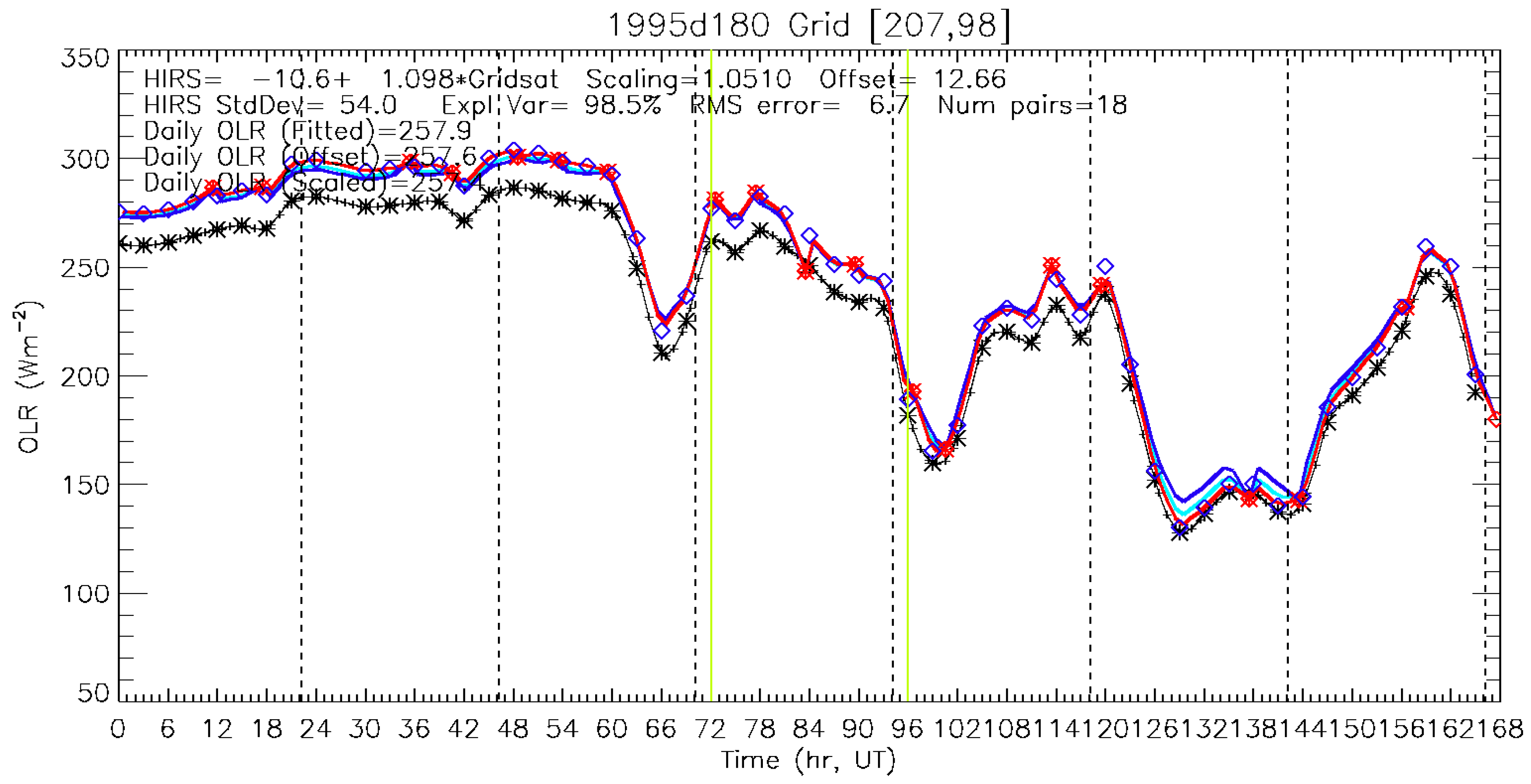
- The Imager OLR data is adjusted (Figure 1, blue diamonds) and now reaches the same absolute radiometric level as in HIRS;
- Imager OLR is combined with HIRS OLR to form a single hourly time series (Figure 1, red curve);
- Trapezoidal rules are applied over all available data (at a 3-hourly or better sampling rate) to derive the integral for the target day. The target day is the center (4th day) of the 7-day boxcar (Figure 1, green vertical lines).
3. Results
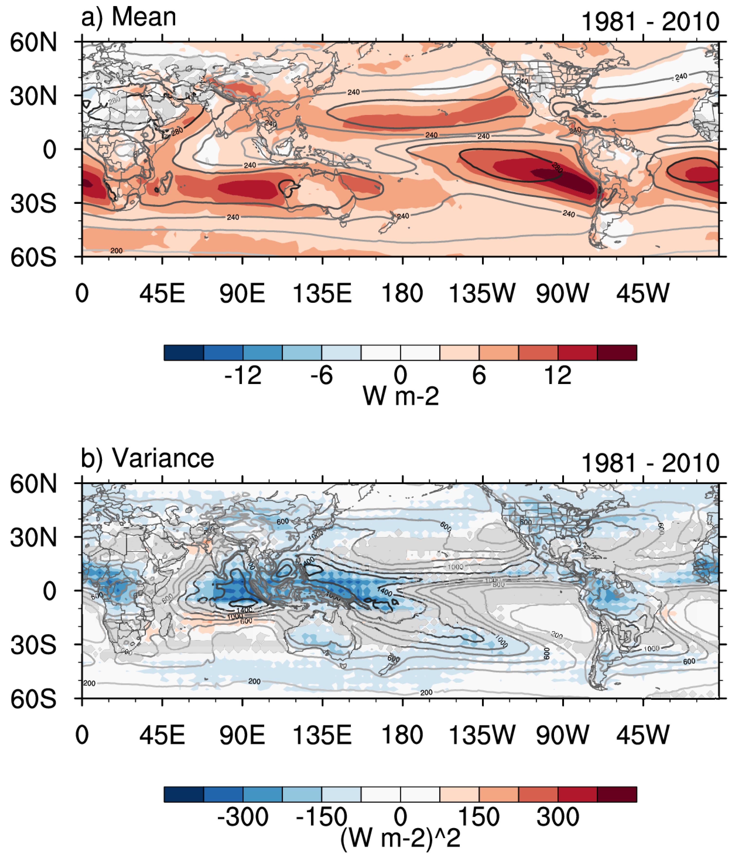
3.1. Validation
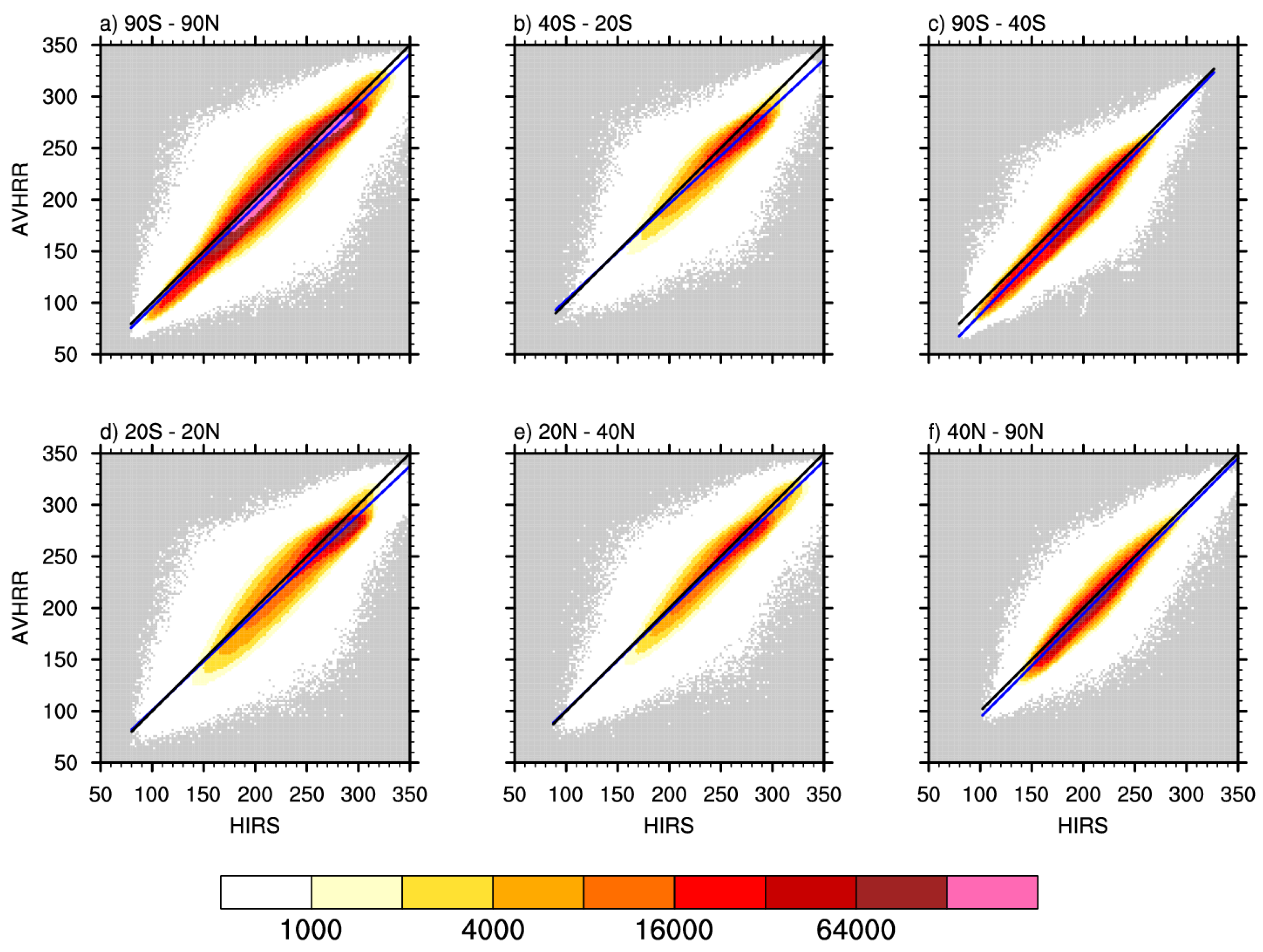
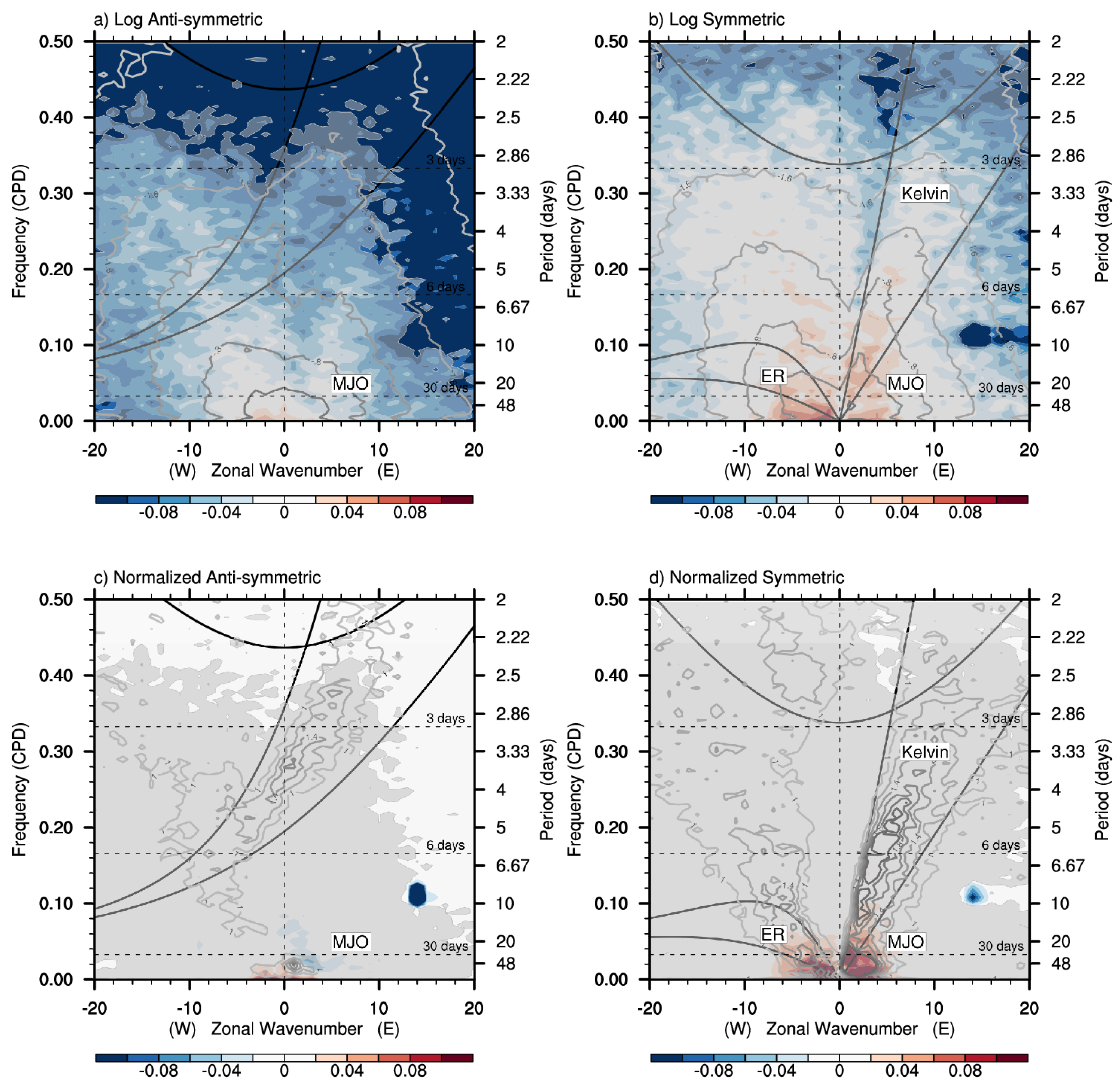
3.2. Comparison
4. Conclusions
Author Contributions
Funding
Acknowledgments
Conflicts of Interest
References
- Liebmann, B.; Smith, C.A. Description of a complete (interpolated) outgoing longwave radiation dataset. Bull. Am. Meteorol. Soc. 1996, 77, 1275–1277. [Google Scholar]
- Ohring, G.; Gruber, A.; Ellingson, R. Satellite determinations of the relationship between total longwave radiation flux and infrared window radiance. J. Climatol. Appl. Meteorol. 1984, 23, 416–425. [Google Scholar] [CrossRef]
- Wheeler, M.; Kiladis, G.N. Convectively coupled equatorial waves: Analysis of clouds and temperature in the wavenumber–frequency domain. J. Atmos. Sci. 1999, 56, 374–399. [Google Scholar] [CrossRef]
- Matsuno, T. Quasi-geostrophic motions in the equatorial area. J. Meteorol. Soc. Jpn. Ser. II 1966, 44, 25–43. [Google Scholar] [CrossRef]
- Lindzen, R.D. Planetary waves on beta-planes. Mon. Weather. Rev. 1967, 95, 441–451. [Google Scholar] [CrossRef]
- Zhang, C. Madden-julian oscillation. Rev. Geophys. 2005, 43, RG2003. [Google Scholar] [CrossRef]
- Madden, R.A.; Julian, P.R. Detection of a 40–50 day oscillation in the zonal wind in the tropical Pacific. J. Atmos. Sci. 1971, 28, 702–708. [Google Scholar] [CrossRef]
- Madden, R.A.; Julian, P.R. Description of global-scale circulation cells in the tropics with a 40–50 day period. J. Atmos. Sci. 1972, 29, 1109–1123. [Google Scholar] [CrossRef]
- Wheeler, M.C.; Hendon, H.H. An all-season real-time multivariate MJO index: Development of an index for monitoring and prediction. Mon. Weather Rev. 2004, 132, 1917–1932. [Google Scholar] [CrossRef]
- National Research Council. Climate Data Records from Environmental Satellites: Interim Report; The National Acadamies Press: Washington, DC, USA, 2004. [Google Scholar]
- Ellingson, R.G.; Yanuk, D.J.; Lee, H.-T.; Gruber, A.A. Technique for estimating outgoing longwave radiation from HIRS radiance observations. J. Atmos. Ocean. Technol. 1989, 6, 706–711. [Google Scholar] [CrossRef]
- Ellingson, R.G.; Lee, H.-T.; Yanuk, D.; Gruber, A. Validation of a technique for estimating outgoing longwave radiation from HIRS radiance observations. J. Atmos. Ocean. Technol. 1994, 11, 357–365. [Google Scholar] [CrossRef]
- Lee, H.-T.; Gruber, A.; Ellingson, R.G.; Laszlo, I. Development of the HIRS outgoing longwave radiation climate dataset. J. Atmos. Ocean. Technol. 2007, 24, 2029–2047. [Google Scholar] [CrossRef]
- NOAA Polar Orbiter Data (POD) User’s Guide: 1998 Version. Available online: https://www1.ncdc.noaa.gov/pub/data/satellite/publications/podguides/TIROS-N%20thru%20N-14/pdf/NCDCPD-ch1.pdf (accessed on 2 August 2018).
- NOAA KLM User’s Guide: February 2009 Version. Available online: https://www1.ncdc.noaa.gov/pub/data/satellite/publications/podguides/N-15%20thru%20N-19/pdf/0.0%20NOAA%20KLM%20Users%20Guide.pdf (accessed on 2 August 2018).
- Lee, H.-T. Climate Algorithm Theoretical Basis Document (C-ATBD): Outgoing Longwave Radiation (OLR)—Daily; CDRP-ATBD-0526; NOAA’s Climate Data Record (CDR) Program: Ashveille, NC, USA, 2014.
- Ba, M.B.; Ellingson, R.G.; Gruber, A. Validation of a technique for estimating OLR with the GOES sounder. J. Atmos. Ocean. Technol. 2003, 20, 79–89. [Google Scholar] [CrossRef]
- Lee, H.-T.; Heidinger, A.; Gruber, A.; Ellingson, R.G. The HIRS outgoing longwave radiation product from hybrid polar and geosynchronous satellite observations. Adv. Space Res. 2004, 33, 1120–1124. [Google Scholar] [CrossRef]
- Kondratovich, V. GOES Surface & Insolation Products (GSIP); version 3.3; National Environmental Satellite, Data, and Information Service, Office of Satellite Data Processing and Distribution: College Park, MD, USA, 2013.
- Lee, H.-T.; Laszlo, I.; Gruber, A. Algorithm Theoretical Basis Document (ATBD): ABI Earth Radiation Budget—Outgoing Longwave Radiation; NOAA NESDIS Center for Satellite Applications and Research (STAR): College Park, MD, USA, 2010.
- Knapp, K.R.; Ansari, S.; Bain, C.L.; Bourassa, M.A.; Dickinson, M.J.; Funk, C.; Helms, C.N.; Hennon, C.C.; Holmes, C.D.; Huffman, G.J.; et al. Globally gridded satellite observations for climate studies. Bull. Am. Meteorol. Soc. 2011, 92, 893–907. [Google Scholar] [CrossRef]
- Lee, H.-T. Climate Algorithm Theoretical Basis Document (C-ATBD): Outgoing Longwave Radiation (OLR)-Monthly; CDRP-ATBD-0097; NOAA’s Climate Data Record (CDR) Program: Asheville, NC, USA, 2017.
- Knapp, K.R. Scientific data stewardship of international satellite cloud climatology project B1 global geostationary observations. J. Appl. Remote Sens. 2008, 2, 023548. [Google Scholar] [CrossRef]
- Gruber, A.; Ellingson, R.; Ardanuy, P.; Weiss, M.; Yang, S.K.; Oh, S.N. A Comparison of ERBE and AVHRR Longwave Flux Estimates. Bull. Am. Meteorol. Soc. 1994, 75, 2115–2130. [Google Scholar] [CrossRef] [Green Version]
- Kiladis, G.N.; Straub, K.H.; Haertel, P.T. Zonal and vertical structure of the Madden–Julian oscillation. J. Atmos. Sci. 2005, 62, 2790–2809. [Google Scholar] [CrossRef]
- Kiladis, G.N.; Wheeler, M.C.; Haertel, P.T.; Straub, K.H.; Roundy, P.E. Convectively coupled equatorial waves. Rev. Geophys. 2009, 47, RG2003. [Google Scholar] [CrossRef]
- Schreck, C.J.; Shi, L.; Kossin, J.P.; Bates, J.J. Identifying the MJO, equatorial waves, and their impacts using 32 years of HIRS upper-tropospheric water vapor. J. Clim. 2013, 26, 1418–1431. [Google Scholar] [CrossRef]
- Bates, J.J.; Jackson, D.L.; Bréon, F.-M.; Bergen, Z.D. Variability of tropical upper tropospheric humidity 1979–1998. J. Geophys. Res. 2001, 106, 32271–32281. [Google Scholar] [CrossRef]
- Lee, H.-T. NOAA Climate Data Record (CDR) of Daily Outgoing Longwave Radiation (OLR), version 1.2; NOAA CDR Program: Asheville, NC, USA, 2014. [Google Scholar] [CrossRef]


© 2018 by the authors. Licensee MDPI, Basel, Switzerland. This article is an open access article distributed under the terms and conditions of the Creative Commons Attribution (CC BY) license (http://creativecommons.org/licenses/by/4.0/).
Share and Cite
Schreck, C.J., III; Lee, H.-T.; Knapp, K.R. HIRS Outgoing Longwave Radiation—Daily Climate Data Record: Application toward Identifying Tropical Subseasonal Variability. Remote Sens. 2018, 10, 1325. https://0-doi-org.brum.beds.ac.uk/10.3390/rs10091325
Schreck CJ III, Lee H-T, Knapp KR. HIRS Outgoing Longwave Radiation—Daily Climate Data Record: Application toward Identifying Tropical Subseasonal Variability. Remote Sensing. 2018; 10(9):1325. https://0-doi-org.brum.beds.ac.uk/10.3390/rs10091325
Chicago/Turabian StyleSchreck, Carl J., III, Hai-Tien Lee, and Kenneth R. Knapp. 2018. "HIRS Outgoing Longwave Radiation—Daily Climate Data Record: Application toward Identifying Tropical Subseasonal Variability" Remote Sensing 10, no. 9: 1325. https://0-doi-org.brum.beds.ac.uk/10.3390/rs10091325