Article

Can Multispectral Information Improve Remotely Sensed Estimates of Total Suspended Solids? A Statistical Study in Chesapeake Bay

by
Nicole M. DeLuca
1,*,
Benjamin F. Zaitchik
1 and
Frank C. Curriero
2
1
Department of Earth and Planetary Sciences, Johns Hopkins University, 3400 N. Charles Street, Olin Hall, Baltimore, MD 21218, USA
2
Department of Epidemiology, Johns Hopkins Bloomberg School of Public Health, Johns Hopkins University, 615 N. Wolf Street, Baltimore, MD 21205, USA
*
Author to whom correspondence should be addressed.
Submission received: 24 July 2018 / Revised: 15 August 2018 / Accepted: 30 August 2018 / Published: 1 September 2018
(This article belongs to the Special Issue Remote Sensing of Ocean Colour)

Abstract

:
Total suspended solids (TSS) is an important environmental parameter to monitor in the Chesapeake Bay due to its effects on submerged aquatic vegetation, pathogen abundance, and habitat damage for other aquatic life. Chesapeake Bay is home to an extensive and continuous network of in situ water quality monitoring stations that include TSS measurements. Satellite remote sensing can address the limited spatial and temporal extent of in situ sampling and has proven to be a valuable tool for monitoring water quality in estuarine systems. Most algorithms that derive TSS concentration in estuarine environments from satellite ocean color sensors utilize only the red and near-infrared bands due to the observed correlation with TSS concentration. In this study, we investigate whether utilizing additional wavelengths from the Moderate Resolution Imaging Spectroradiometer (MODIS) as inputs to various statistical and machine learning models can improve satellite-derived TSS estimates in the Chesapeake Bay. After optimizing the best performing multispectral model, a Random Forest regression, we compare its results to those from a widely used single-band algorithm for the Chesapeake Bay. We find that the Random Forest model modestly outperforms the single-band algorithm on a holdout cross-validation dataset and offers particular advantages under high TSS conditions. We also find that both methods are similarly generalizable throughout various partitions of space and time. The multispectral Random Forest model is, however, more data intensive than the single band algorithm, so the objectives of the application will ultimately determine which method is more appropriate.

Graphical Abstract

1. Introduction

Total suspended solids (TSS) is an important parameter to monitor in estuarine systems due to its ecological, economic, and human health impacts. Suspended solids in a water column reduce light and other radiation availability for phytoplankton and submerged aquatic vegetation (SAV) growth, while increased sedimentation rates reduce benthic organism habitability. It has also been shown that the volume of suspended particles in water may have biological importance for predicting incidence and abundance of pathogenic bacteria like Vibrio parahaemolyticus [1,2,3]. Forms of suspended particles that contribute to TSS concentrations include sediment, detrital matter, and microorganisms. The type of sediment and organics in a water body can vary widely by region because they are introduced into the water column through processes that include watershed inputs, resuspension of bottom sediments, and ecological productivity.
It can be impractical to monitor TSS in situ at a resolution sufficient for studying sediment plume dynamics, monitoring and forecasting algal blooms, or modeling pathogenic bacteria, due to both the cost and time involved in in situ sampling and to the sometimes prohibitive logistics of installing dense monitoring networks. Remotely sensed TSS estimates can be a useful alternative. Many satellite-derived and in situ-measured radiance algorithms for estuarine TSS retrieval have been developed based on the observed correlation between TSS and reflectances in the red and near-infrared red (NIR) wavelengths [4,5,6,7,8,9,10,11,12,13,14,15,16]. Use of these bands is a particular advantage for studies that use the Moderate Resolution Imaging Spectroradiometer (MODIS), due to the higher spatial resolution of those bands on MODIS. This can be useful in geographically complex estuarine environments with small-scale dynamics and regions of interest near the shoreline. Many of these TSS algorithms are tuned to a specific site or region, since differences between water bodies in inorganic and organic particle types and sizes change the inherent optical properties (IOPs) of the water [17,18].
Some TSS algorithms employ a switching function to swap between the red and NIR bands in accordance with some radiance threshold in order to account for a larger range of TSS values [13,14]. Other ocean color remote sensing studies have found that two-band differencing approaches are effective algorithms for similar applications [19]. Fewer studies have explored relationships between TSS concentration and optical properties in wavelengths outside of the red and NIR ranges for TSS algorithm development in estuarine environments [20,21]. This has historically been due to both the limits of spatial resolution in other visible bands and the non-negligible scattering from phytoplankton pigments and water at wavelengths less than 580-nm [22,23]. However, the use of shorter wavelengths may be beneficial for estimation of low TSS concentrations due to the higher signal-to-noise ratio that offers higher sensitivity to suspended particles than longer wavelengths provide.
Chesapeake Bay in the eastern United States has been used as a test bed for numerous studies relating to water quality because of an extensive and continuous in situ sampling network that spans multiple decades. It is the largest estuary in the United States, with a 165,800 square kilometer (64,000 square mile) watershed including six states [24]. Over 150 major rivers and tributaries feed freshwater from the watershed into the estuary, the largest of which is the Susquehanna River in the northernmost reaches. Increasing sediment and nutrient loads in tributary runoff have significantly hindered the ecological health and productivity of the Chesapeake Bay since the onset of agriculture in the region [25]. More recently, continued degradation of the estuary’s health has prompted legislative action under the Clean Water Act in the form of Total Maximum Daily Load (TMDL) targets [26]. Remote sensing can aid in situ monitoring efforts to follow improvements or declines in Chesapeake Bay ecosystem health influenced by sediment loads.
This study uses the Chesapeake Bay as a test case to investigate whether remotely sensed TSS estimates can be improved by utilizing additional MODIS Aqua bands alongside the commonly used red and NIR bands. Eight statistical and machine learning models, using 11 of MODIS Aqua’s visible and NIR bands as predictor variables, are evaluated for their prediction performance using Chesapeake Bay Program (CBP) in situ TSS measurements over years 2003 to 2016. TSS predictions from the best performing model are then compared to those from a single-band algorithm that is widely used for remotely sensed TSS retrieval in the Chesapeake Bay. Utilization of additional sensor bands can potentially improve satellite TSS retrievals in optically complex estuarine systems like the Chesapeake Bay. At the same time, highly multispectral sensors are expensive to build and to fly relative to sensors with fewer bands, so it is useful to understand if and how the addition of spectral bands contributes to environmental monitoring of TSS and other parameters.

2. Materials and Methods

2.1. Data Description

2.1.1. Satellite Data Processing

Daily Level 1A MODIS Aqua (R2014.0.2) ocean color products for the Chesapeake Bay were downloaded from NASA’s ocean color archive (http://ocean color.gsfc.nasa.gov/) for years 2003 through 2016 for statistical and machine learning model analyses, and 2017 for mapped comparisons [27]. All images were batch processed from Level 1 to Level 2 with NASA’s SeaDAS 7.4 software using the standard iterative NIR atmospheric correction at 1-km resolution [28]. Instead of the default cloud mask we used the 2130 nm band for cloud detection with a threshold albedo of 0.018 [29]. We also turned off the Level 2 high light mask so that pixels in which the NIR bands saturate or nearly saturate, which is common for regions of high turbidity, would be included in the output [10,29]. The Level 2 stray light mask removes pixels adjacent to bright objects such as clouds and land due to possible light contamination. However, the default setting in SeaDAS may be too conservative for an estuarine system like the Chesapeake Bay. To avoid removing crucial areas around clouds or near shorelines, we decreased the SeaDAS stray light mask to a 3 by 3 array [29]. This procedure produced all of the Level 2 MODIS data, including remote sensing reflectance (Rrs) and normalized water leaving radiance (nLw) products, used in the subsequent analyses (Table 1).

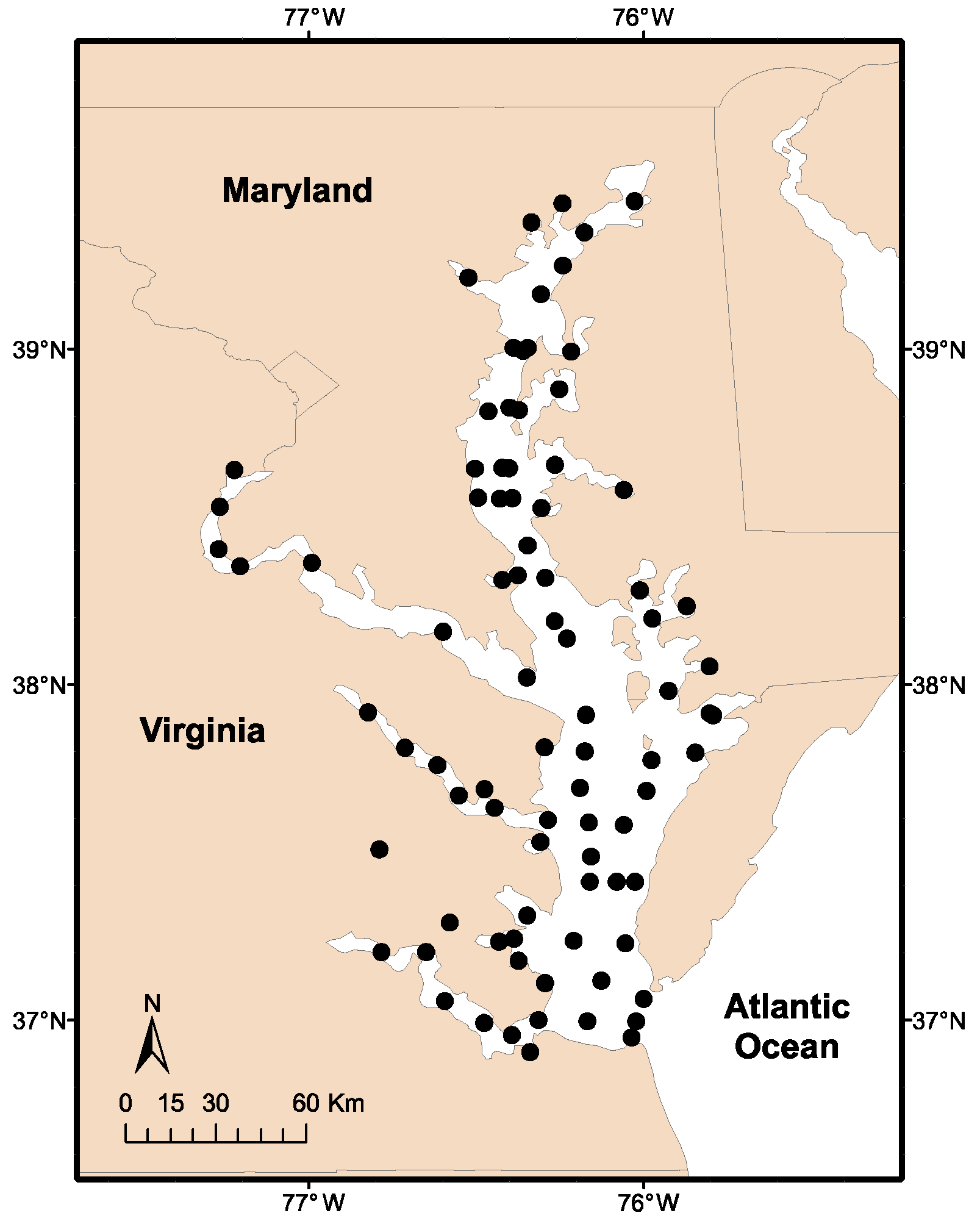
2.1.2. In situ Measurements

In situ TSS measurements used in this study for years 2003 to 2016, and subsequently 2017 for mapped comparisons, were downloaded from the Chesapeake Bay Program’s online water quality database (http://datahub.chesapeakebay.net) [30]. This online database is a collection of bi-monthly water quality measurements taken by state and federal agencies at predetermined stations throughout the Chesapeake Bay (Figure 1). In situ TSS measurements in this database are determined according to the procedure from U.S. EPA method 160.2. Only the measurements taken within the top 1 m of the water column were used for these analyses [10,31].

2.1.3. Satellite-in Situ Matchups

In situ measurements were matched with same-day processed MODIS pixels within 250 meters of the in situ station’s coordinates using a geographical distance matrix in the R package “fields” of the R Statistical Computing Environment [32,33]. Over the 16-year period, we created a dataset of 1360 satellite-in situ matchups found on 490 unique days. Statistics for this matchup dataset are found in Table 1. The 490 days include representative data from all seasons and years, giving us a comprehensive dataset from which to conduct our analyses. There is thought to be no more than a few hours between satellite overpass and in situ sampling times for most matchups because Chesapeake Bay Program sampling for 2003–2016 occurs most frequently during late-morning (Figure S1) while MODIS overpasses occur in the early afternoon. TSS can change within a few hours under storm conditions and in smaller tributaries, but the temporal proximity of the matchups is adequate under most weather conditions and away from the shore. It is also consistent with the matchup criteria used in previous studies [10]. Our satellite-in situ dataset also includes eighty-six unique matchup locations that cover a large portion of the Chesapeake Bay spatially, including both the Mainstem and several large tributaries (Figure 1).
Where one or more MODIS bands are saturated in our matchup dataset due to high surface reflectance or incompatibilities with the atmospheric correction method, missing values are present in the vectors of predictor variables. Because it is necessary to omit missing values in order to run many of our modeling approaches, all satellite-in situ matchups where these missing values occur were excluded from the dataset. This trimming of missing predictor values resulted in 36% of the raw satellite-in situ matchup dataset (n = 2111) being excluded from the final matchup dataset (n = 1360) used for analyses. After this incomplete data was removed (including in situ TSS values up to 137.0 mg/L), the range of in situ measured TSS used in our analyses was limited to 2.18 to 47.0 mg/L (Table 1).

2.2. Methods

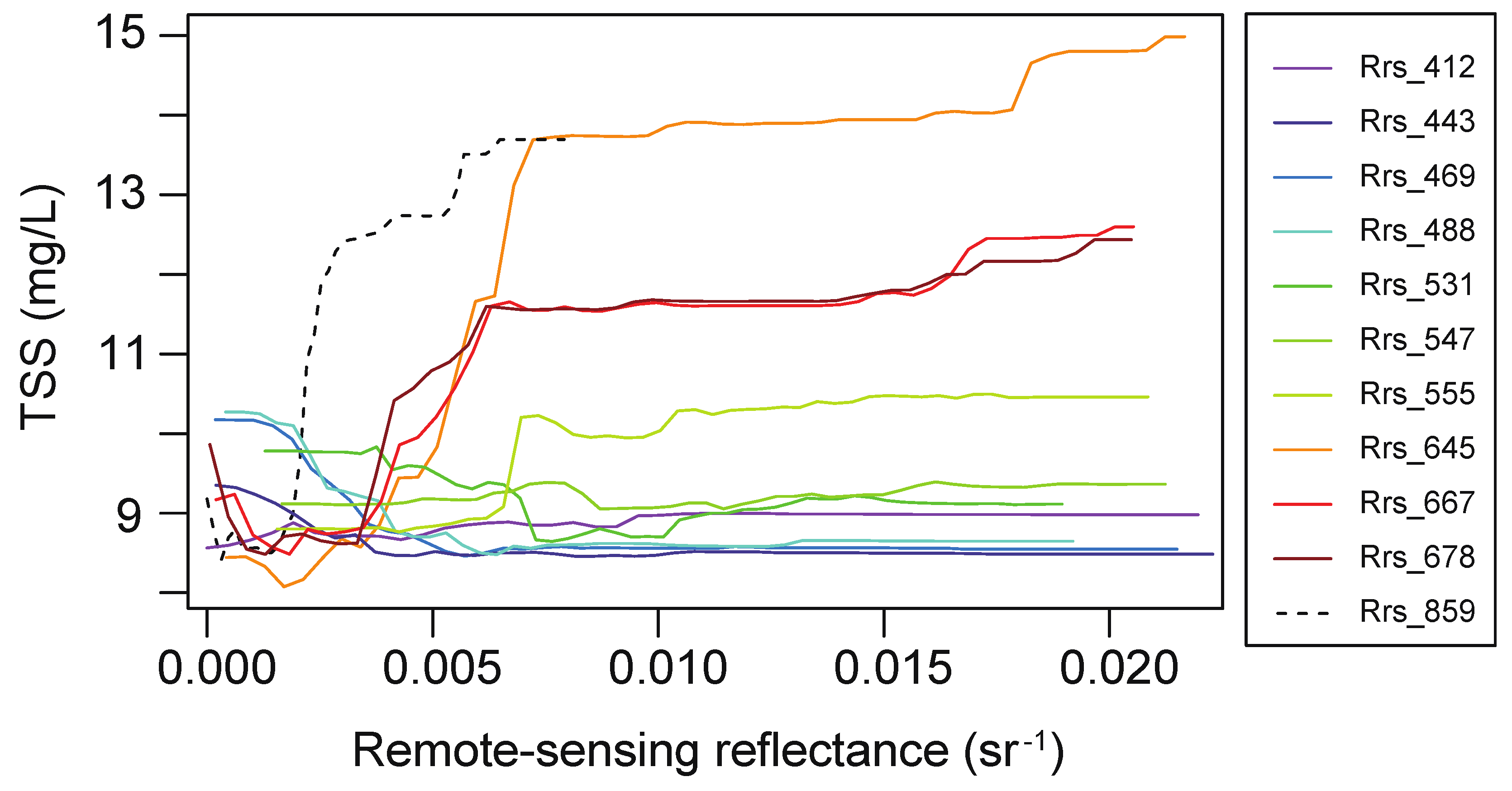
2.2.1. Statistical Methodology

Following a procedure outlined by Urquhart et al. 2012 [31], eight statistical and machine learning models were evaluated for empirically estimating total suspended solids in the Chesapeake Bay using satellite-derived ocean color products. The 11 MODIS remote-sensing reflectances (Rrs) used as predictor variables in these models are summarized in Table 1. We randomly split our dataset of 1360 satellite-in situ matchups into 80% training data and 20% holdout data for cross-validation. We evaluated the predictive performance of our models using three metrics–mean absolute error (MAE), mean square error (MSE), and root mean square error (RMSE). The absolute error gives equal weight to all errors while the two square error metrics give more weight to larger errors or outlier points, with RMSE having the same units as MAE for better comparison. All statistical and machine learning modeling and subsequent computations were done in R Statistical Computing Environment software (version 3.3.2) [33].

2.2.2. Statistical and Machine Learning Models

Eight statistical and machine learning models were chosen for their ability to regress non-parametric, high dimensional data with a continuous response variable. The remote-sensing reflectances (Rrs) from 11 MODIS-Aqua bands used for ocean color and land remote sensing are used as the predictor variables in these models, while TSS concentration is the response variable.
We included three types of decision tree regression models: Classification and regression tree (CART) [34], Bayesian additive regression tree (BART) [35], and Random Forest (RF) [36]. These tree-based models follow rules at data-defined nodes in the covariates to predict output of the response variable. The RF model uses a large number of trees, thereby creating a “forest” and determines output based on the most commonly used decision path for the dataset.
A generalized linear model (GLM) modifies the standard ordinary least squares linear regression model by adding a link function that can account for non-normal distributions of response data [37]. We use a logarithmic link function for our GLM based on the log-normal distribution of TSS measurements in our dataset. Our generalized additive model (GAM) [38] works similarly to the GLM, but accounts for possible non-linear effects of the predictors on the response by first using a smoothing function on the predictor variables. The Multivariate Adaptive Regression Spline (MARS) [39] model is also similar to a GLM, but the number and type of link functions are automatically determined for the given dataset.
Neural networks (NN) take their name from their resemblance to the interactions of neurons and synapses in the brain. A layer of input data consisting of predictor variable data are sent to a predetermined number of hidden layers through connections, for which weights are calculated. When the sum of a connection’s weights reaches a given threshold, the connection “fires” like a synapse and continues to the output data layer [40].
Support Vector Machines (SVM) find a regression fit by using a scaled-linear contribution from data whose residuals fall outside of a user-specified threshold, while data whose residuals are within the threshold do not contribute to the fit [41].
All 11 predictor variables (MODIS-Aqua bands) are retained in the training phase of model development except for in two models. The CART model only finds 645-nm, 667-nm, and 412-nm to be significant predictor variables for tree splitting, while the MARS model excludes the 443-nm, 488-nm, 547-nm and 667-nm predictors. Forcing these models to use all 11 predictors presents the risk of overfitting, which would decrease their performance on the holdout cross-validation dataset.
Prediction errors from the eight models (models fit on the training set and predictions generated for the hold out sample) were compared to each other and to a mean statistical null model, which was a model containing only the mean of the TSS response variable for all predictions. p-Values were calculated for each pair-wise comparison for MAE and MSE and corrected for multiple comparisons using the Holm method to test for statistical significance [42].
TSS predictions from the best performing model were then compared to those from the optically based, single-band algorithm presented in Ondrusek et al. 2012 [10] (referred to as O-2012 henceforth) for the same satellite-in situ matchups. The O-2012 algorithm uses MODIS normalized water leaving radiance (nLw) at 645-nm and is commonly used for estimating TSS in the Chesapeake Bay. It was derived using in situ-measured optical data from only the mid-Chesapeake Bay in 2008 within a few hours of satellite overpass. The authors fit the following 3rd order polynomial function to their data to relate in situ nLw (645) to 35 in situ total suspended matter samples ranging from 4.50 to 14.92 mg/L:
TSM(mg L−1) = 3.8813(nLw(645))3 − 13.822(nLw(645))2 + 19.61(nLw(645))
The algorithm was validated using 270 matchups between MODIS pixels and Chesapeake Bay Program in situ TSS data from 2009 with concentrations up to 100 mg/L. The authors found a mean percent difference of −4.2% and a mean absolute percent difference of 36%.

2.2.3. Geographic and Temporal Cross-Validation

A common criticism of empirical remote sensing models is that they are not generalizable throughout space and time when they are trained on a comprehensive dataset. In order to test the ability of the model to deal with variable sediment distributions between the Mainstem of the Chesapeake Bay and its tributaries as well as missing data due to cloud cover, we trained our highest performing model on one region or time period and tested its performance on another region or time period. To do this, we divided our satellite-in situ matchup dataset into various training datasets based on latitude, longitude, region and time of year. Dataset partitions include East and West based on a selected longitude, North and South based on a selected latitude, Mainstem and tributaries of the estuary, and the high and low flow discharge seasons. We compared the MAE, MSE, and RMSE of our best model on the corresponding holdout datasets to that of O-2012 for the same holdout datasets to test our model’s ability to predict TSS in the Chesapeake Bay as successfully as a single-band, optically-based algorithm.

3. Results and Discussion

3.1. Model Comparison

All eight statistical and machine learning models in this study outperformed the mean statistical null model in MAE and RMSE (Table 2). They were also statistically significant in MAE compared to the mean statistical null model based on a Holm multiple comparisons correction. This suggests that our eight models provide more information than assuming the mean of the dataset.
Of our eight models tested in this study, the Random Forest had the lowest MAE of 2.42, followed by the SVM with MAE of 2.57, the GAM with MAE of 2.64, and the GLM with MAE of 2.69 (Table 2). The RF model also had the best square error predictive accuracy with RMSE of 4.36, followed by the GAM with RMSE of 4.53, the BART with RMSE of 4.66, and MARS with RMSE of 4.69 (Table 2).
In order to better understand how the RF model predicts TSS in our holdout dataset, we looked at each predictor’s contribution to the model through partial dependence plots [43]. Partial dependence plots are valuable tools for interpreting predictive machine learning models like a Random Forest in which the relationships between predictors and response are not intuitive. They allow visualization of the amount of change in predicted response a given predictor variable produces when all other predictors in the model are averaged.
The partial dependence plots for all 11 MODIS bands in the RF model are shown in Figure 2. The red (645-nm, 667-nm, and 678-nm) and NIR (859-nm) bands play the largest role in predicting higher TSS values, which reflects the use of the red and NIR bands used in many TSS algorithms’ development [4,5,6,7,8,9,10,11,12,13,14,15,16]. Several of the blue (496-nm, 448-nm and 443-nm) and green (531-nm and 555-nm) bands appear to be important to predicting lower ranges of TSS. These results suggest that while most algorithms use the “red-ness” of sediment to remotely sense TSS concentrations, it could also be beneficial to use the “blue-ness” of clearer waters in developing algorithms to estimate TSS via satellite. The partial dependence plots also showed that the 412-nm, 443-nm, and 547-nm bands contribute very little to the RF model, shown by the lack of variation in TSS prediction over the respective ranges of remote-sensing reflectances (Figure 2). Pruning the RF model by excluding these three MODIS bands decreased the MAE and RMSE (2.38 and 4.30, respectively). The RF model referred to in the study henceforth is the pruned RF model that includes only 8 MODIS bands.

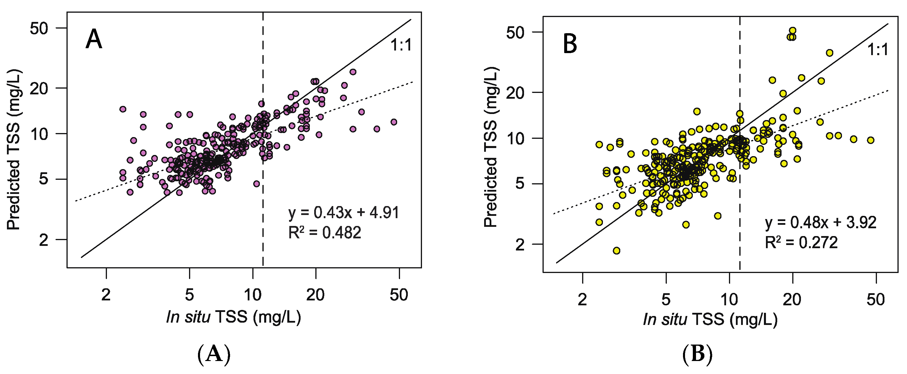
3.2. Comparison with Single-Band TSS Algorithm

We compared our top performing model, a Random Forest that was pruned to minimize error in MAE, MSE and RMSE, to the O-2012 for the holdout validation dataset. The O-2012 algorithm was applied with its published coefficients, as that is the version commonly used in Chesapeake Bay applications. We also generated a version of the same polynomial form but with updated coefficients and without the y-intercept being forced through zero (referred to as O-2012(fit)), fit using the training and evaluation datasets used for our other models:
TSM(mg L−1) = 19.222(nLw(645))3 − 10.293(nLw(645))2 + 115.539(nLw(645)) + 8.467
This customized polynomial model showed an improvement over the standard O-2012 algorithm in our holdout validation test, which may be due to the larger range of TSS concentrations used to train our polynomial regression. However, the RF model using multiple bands still had better performance than the newly fitted O-2012(fit) using a single band (Table 3). Since O-2012 and O-2012(fit) show nearly identical performance and have similar behavior across geography and TSS concentrations, we focus on the original, published O-2012 algorithm through the rest of our analysis.
The RF model produces significantly lower errors from the O-2012 algorithm in both MAE and MSE (Table 3). The RF model also introduces less bias (mean error of −0.04) in the holdout cross-validation than O-2012 (mean error of −0.54). The RF model’s MAE accounts for 5.3% of the range in TSS values used in this study (2.4 to 47.0 mg/L), while O-2012’s MAE accounts for 6.6%. The accuracy necessary for each user’s application may indicate whether either, or both, methods have acceptable performance for TSS estimation.
In order to assess the effect of the algorithmic approach (machine learning versus polynomial regression) we also compared a Random Forest model using only the same remote sensing reflectance in 645-nm as in the O-2012 algorithm. The single-band RF model, referred to as RF(645), performed better in MAE (2.76 vs. 2.97) and RMSE (4.57 vs. 5.61) than O-2012 and better in RMSE (4.56 vs. 4.67) than O-2012(fit) for the holdout cross-validation. This indicates that the application of machine learning alone provides some advantage over the polynomial method. The use of multiple bands provides further improvement (Table 3).
The one-to-one regressions for in situ measured TSS to predicted TSS for the pruned RF model and O-2012 algorithm show that higher TSS values are not predicted as well as lower TSS values for either prediction method (Figure 3). The pruned RF model consistently underestimates the higher range of TSS values, which may be due to the log-normal distribution of the response variable in our training dataset. More data in a higher TSS range in the training dataset may allow the model to better predict higher TSS values, but could come at the cost of not predicting the more frequently measured lower range as accurately. There is a wide spread in predictions for these high TSS events using O-2012.
To better investigate this lack of prediction skill in both the RF model and O-2012 algorithm at higher ranges of TSS, we compared the error for both models for holdout data above the 80th percentile (TSS > 11.3 mg/L, n = 55) (Figure 3). On high TSS values, the RF model had a lower MAE of 5.16 than O-2012, with MAE of 8.33 (Table 4). The RF model also had a lower RMSE than O-2012, 8.24 vs. 11.71, respectively. The RF model’s MAE and MSE error metrics are significantly lower than the O-2012 algorithm’s error metrics to the 95% confidence interval (Table 4). The RF model and O-2012 have similar bias (mean error of 4.50 and 4.51, respectively) for the high TSS range predictions. These results suggest that the RF model is able to better predict TSS values farther from the mean than O-2012, although both methods produce larger errors for higher TSS ranges.
It is also important to compare how the two models perform below the 80th percentile (TSS < 11.3 mg/L, n = 217) because it represents more commonly measured TSS values in the Chesapeake Bay. We find that the RF model and O-2012 perform very similarly for MAE (Table 4). The O-2012 algorithm performs better than the RF model for MSE, 4.67 and 5.92 respectively (Table 4). However, neither MAE nor MSE from the two methods are significantly different at the 0.05 level for this lower TSS holdout validation data (Table 4).

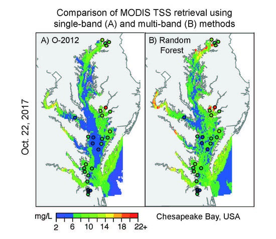
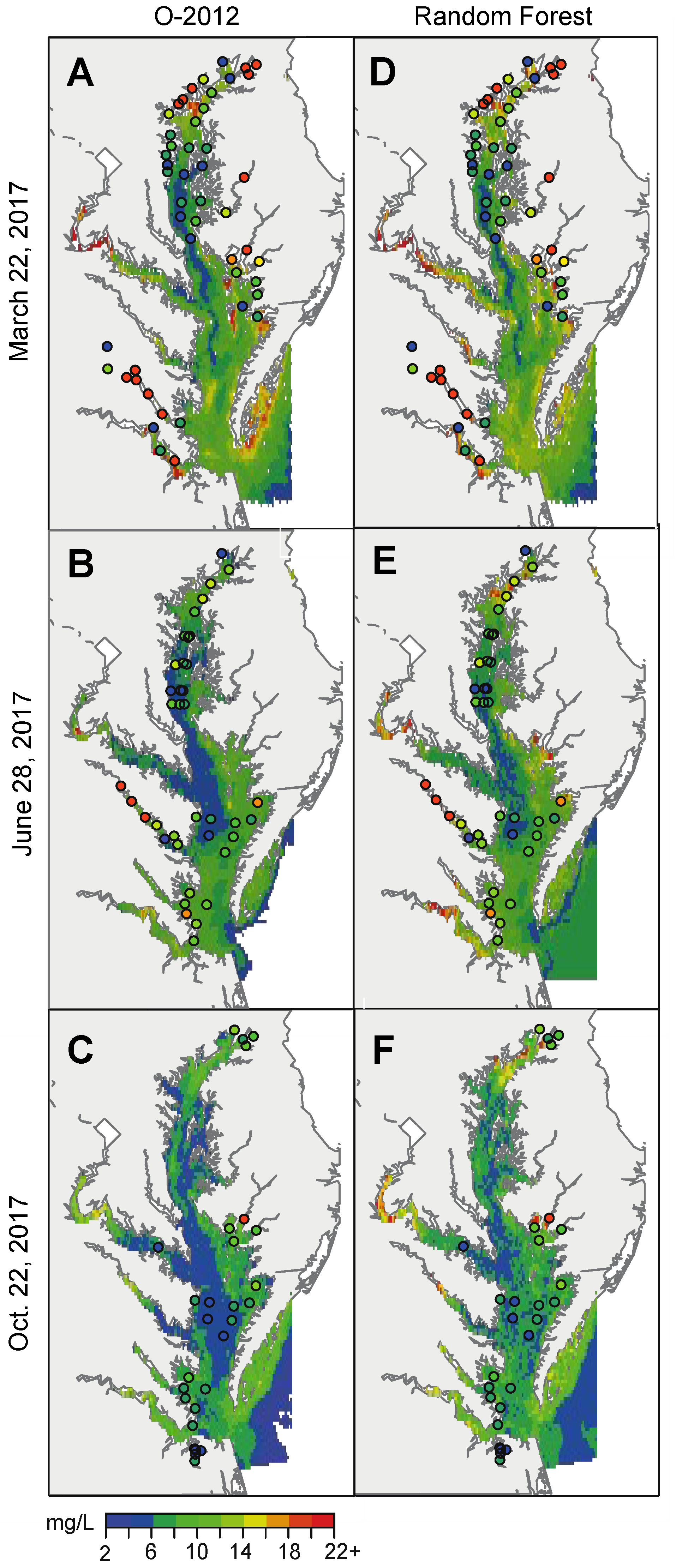
3.3. Daily Satellite, in situ Mapped Comparisons

In order to compare the performance of the RF and O-2012 methods in space, we predicted remotely sensed TSS using each method on data that was not included in either the training dataset or holdout validation dataset. Figure 4 shows three MODIS images from 2017 dates with good spatial coverage of Chesapeake Bay from three seasons: (1) 22 March 2017 in the spring, (2) 28 June 2017 in the summer, and (3) 22 October 2017 in the fall. In situ measurements from the same, previous, or subsequent day (in order to increase the number of comparison points) are also shown for comparison between remotely sensed and in situ measured TSS. Satellite-in situ matchups were determined by the same method outlined in Section 2.1.3.
Overall, Figure 4 shows that both the RF model and O-2012 capture the general structure of TSS across the Bay in these randomly selected matchups. However, relative performance in MAE, MSE, and RMSE depends on the date chosen. In general, O-2012 offers more consistent performance in the lower Mainstem for the three dates shown. In the upper Mainstem and tributaries, the RF model generally performs better than O-2012 for the summer and fall dates, but not for the spring date. The differences in performance between the two methods are not statistically significant in MAE or MSE for any of the regions (upper Mainstem, lower Mainstem, and tributaries) on any of the dates.

3.4. Geographic and Temporal Cross-Validation

In order to test whether our top performing model was generalizable in predicting TSS throughout the Chesapeake Bay, we tested the performance of the RF model for various training and holdout datasets. We then compared the generalizability of the RF model to that of O-2012 for the same holdout datasets using MAE and MSE metrics. The naming convention works similarly to the following example: “East for West” indicates that the model is trained on a dataset encompassing stations only on the Eastern side of the Chesapeake Bay and the holdout validation dataset is comprised of the remaining stations on the Western side.
The results of the geographical and temporal cross-validation are presented in Table 5. Neither the RF model nor the O-2012 algorithm consistently outperforms the other in terms of MAE across the different validation scenarios. Based on MSE however, which gives more weight to larger errors, the RF model performs better than O-2012 in all but one scenario, West for East, and many of the differences between methods are statistically significant. Both methods were more accurate when predicting the East, South, and Mainstem sub-datasets than they were in other regions, and both also had higher skill for holdout predictions in the low discharge season. Both methods are generally similar overall in the accuracy of their predictions across various spatial and temporal partitions of the dataset, even though some differences have statistical significance. Again, the application may determine what level of accuracy or precision is needed in TSS estimations.

4. Conclusions

This study investigates whether additional information can be gained from statistical and machine learning models that utilize multispectral MODIS information when predicting TSS in estuarine systems, using the Chesapeake Bay as a case study. Eight models using 11 MODIS bands, as well as a single-band algorithm, were evaluated for their performance on predicting TSS measurements taken in situ over a 14-year time period throughout the estuary. The Random Forest model performed best out of the eight models and the single-band algorithm on the holdout validation dataset. It also outperformed the single-band algorithm on the top 20th percentile of test data, but did not perform better on the lower 80th percentile. We found that both methods of TSS prediction were generalizable throughout space and time, with relative performance dependent on the error metric used for comparison.
The results of this study suggest that the single-band O-2012 algorithm is a valuable tool for estimating TSS via remote sensing in the Chesapeake Bay for general environmental applications. However, for applications where more accuracy or precision in waters with higher TSS concentrations may be needed, such as when modeling Vibrio bacteria [3], a statistical or machine learning model that utilizes additional MODIS bands could prove valuable. In estuarine systems, additional MODIS bands could provide information about suspended particles other than sediment that contribute to a TSS measurement, such as phytoplankton and detrital matter. Determining the supplementary bands to be added to statistical or machine learning models could vary from estuary to estuary based on the watershed characteristics, biology, and corresponding optical properties of each system. A recent study by Hasan et al. 2017 [15] found that it is beneficial to determine the relationship between reflectance and TSS concentration separately for the Mainstem and tributaries of the Chesapeake Bay, which may account for variability in the optical properties between the two estuarine features. This poorly characterized variability between regions of the estuary may be why a decision tree-based model like a Random Forest better predicts the high TSS values typically found in tributaries.
However, it is important to recognize the utility of a single-band, optically based algorithm like O-2012. These algorithms are generally easier to use for conventional applications of remotely sensed TSS estimates, and their physical basis is more straightforward [16]. In a comprehensive quantitative review of published TSS algorithms, Dorji et al. 2016 [44] found that optically based algorithms generally perform better than empirical algorithms in waters with unknown composition.
Another noteworthy ability of the O-2012 algorithm and other red and NIR algorithms is that of having higher spatial resolution. While red and NIR algorithms can provide 250-m resolution, using other MODIS wavelengths limits spatial resolution to 1-km. This could be a significant disadvantage to using other MODIS bands in a model when near-shore TSS estimates are important. However, recently launched ocean color sensors like the Ocean and Land Colour Instrument (OLCI) provide improved spatial resolution at 300-m resolution bands outside of the red and NIR wavelengths. Therefore, this MODIS study could provide a foundation for multispectral TSS retrieval in higher spatial resolution using newer sensors.
Overall, our results suggest that the application of multispectral data using statistical and machine learning methods to estimate TSS in Chesapeake Bay may offer an increase in skill over standard single-band approaches. It may be particularly useful in regions that often experience higher TSS levels than the lower Mainstem region. However, the existing single-band O-2012 algorithm does perform reasonably well when compared to our best-performing multispectral RF model in Bay-wide evaluations, performing particularly well in lower TSS regions. The relative performance of the two models appears to be sensitive to sub-region, date, and the error metric being evaluated. For this reason, we conclude that the use of additional MODIS bands outside of the red and NIR wavelengths can be utilized to aid in satellite-derived TSS retrieval in estuaries like the Chesapeake Bay, but that the decision on whether adopt such an approach will depend on the objectives of the application.

Supplementary Materials

The following are available online at https://0-www-mdpi-com.brum.beds.ac.uk/2072-4292/10/9/1393/s1, Figure S1: Histogram of sampling times for all Chesapeake Bay program TSS data at or above 1 m depth for years 2003–2016.

Author Contributions

N.M.D. worked on study conceptualization and design, data analysis and writing the manuscript. B.F.Z. advised study conceptualization and design, data analysis, and writing. F.C.C. contributed to data interpretation and revision during the writing process.

Funding

This research was funded by the National Institutes of Allergy and Infectious Diseases (grant No. 1R01AI123931-01A1 to F.C.C. [principal investigator]). Additional support was provided to N.M.D. through The National Science Foundation’s Water, Climate, and Health Integrative Education and Research Traineeship.

Acknowledgments

We thank two anonymous reviewers for their insightful comments and suggestions that added great value to the manuscript. We thank Bruce Monger for his guidance with satellite data processing and Richard Stumpf for his expertise and feedback.

Conflicts of Interest

The authors declare no conflict of interest.

References

  1. Caburlotto, G.; Haley, B.J.; Lleò, M.M.; Huq, A.; Colwell, R.R. Serodiversity and ecological distribution of Vibrio parahaemolyticus in the Venetian Lagoon, Northeast Italy. Environ. Microbiol. Rep. 2010, 2, 151–157. [Google Scholar] [CrossRef] [PubMed]
  2. Johnson, C.N.; Bowers, J.C.; Griffith, K.J.; Molina, V.; Clostio, R.W.; Pei, S.; Laws, E.; Paranjpye, R.N.; Strom, M.S.; Chen, A.; et al. Ecology of Vibrio parahaemolyticus and Vibrio vulnificus in the Coastal and Estuarine Waters of Louisiana, Maryland, Mississippi, and Washington (United States). Appl. Environ. Microbiol. 2012, 78, 7249–7257. [Google Scholar] [CrossRef] [PubMed]
  3. Davis, B.J.K.; Jacobs, J.M.; Davis, M.F.; Schwab, K.J.; DePaola, A.; Curriero, F.C. Environmental determinants of Vibrio parahaemolyticus in the Chesapeake Bay. Appl. Environ. Microbiol. 2017, 83, e01147-17. [Google Scholar] [CrossRef] [PubMed]
  4. Stumpf, R.P. Sediment transport in Chesapeake Bay during floods: Analysis using satellite and surface observations. J. Coastal Res. 1988, 4, 1–15. [Google Scholar]
  5. Hu, C.; Chen, Z.; Clayton, T.; Swarzenski, P.; Brock, J.; Muller-Karger, F. Assessment of estuarine water-quality indicators using MODIS medium-resolution bands: Initial results from Tampa Bay, FL. Remote Sens. Environ. 2004, 93, 423–441. [Google Scholar] [CrossRef]
  6. Doxaran, D.; Ehn, J.; Bélanger, S.; Matsuoka, A.; Hooker, S.; Babin, M. Optical characterisation of suspended particles in the Mackenzie River plume (Canadian Arctic Ocean) and implications for ocean colour remote sensing. Biogeosciences 2012, 9, 3213–3229. [Google Scholar] [CrossRef] [Green Version]
  7. Wang, H.; Hladik, C.M.; Huang, W.; Milla, K.; Edmiston, L.; Harwell, M.A.; Schalles, J.F. Detecting the spatial and temporal variability of chlorophyll-a concentration and total suspended solids in Apalachicola Bay, Florida using MODIS imagery. Int. J. Remote Sens. 2010, 31, 439–453. [Google Scholar] [CrossRef]
  8. Chen, S.; Huang, W.; Chen, W.; Chen, X. An enhanced MODIS remote sensing model for detecting rainfall effects on sediment plume in the coastal waters of Apalachicola Bay. Mar. Environ. Res. 2011, 72, 265–272. [Google Scholar] [CrossRef] [PubMed]
  9. Zhao, H.; Chen, Q.; Walker, N.D.; Zheng, Q.; MacIntyre, H.L. A study of sediment transport in a shallow estuary using MODIS imagery and particle tracking simulation. Int. J. Remote Sens. 2011, 32, 6653–6671. [Google Scholar] [CrossRef]
  10. Ondrusek, M.; Stengel, E.; Kinkade, C.S.; Vogel, R.L.; Keegstra, P.; Hunter, C.; Kim, C. The development of a new optical total suspended material algorithm for the Chesapeake Bay. Remote Sens. Environ. 2012, 119, 243–254. [Google Scholar] [CrossRef]
  11. Feng, L.; Hu, C.; Chen, X.; Song, Q. Influence of the three gorges dam on total suspended matters in the Yangtze estuary and its adjacent coastal waters: Observations from MODIS. Remote Sens. Environ. 2014, 140, 779–788. [Google Scholar] [CrossRef]
  12. Shen, F.; Zhou, Y.; Peng, X.; Chen, Y. Satellite multi-sensor mapping of suspended particulate matter in turbid estuarine and coastal ocean, China. Int. J. Remote Sens. 2014, 35, 4173–4192. [Google Scholar] [CrossRef]
  13. Dogliotti, A.I.; Ruddick, K.G.; Nechad, B.; Doxaran, D.; Knaeps, E. A single algorithm to retrieve turbidity from remotely-sensed data in all coastal and estuarine waters. Remote Sens. Environ. 2015, 156, 157–168. [Google Scholar] [CrossRef]
  14. Han, B.; Loisel, H.; Vantrepotte, V.; Mériaux, X.; Bryére, P.; Ouillon, S.; Dessailly, D.; Xing, Q.; Zhu, J. Development of a semi-analytical algorithm for the retrieval of suspended particulate matter from remote sensing over clear to very turbid waters. Remote Sens. 2016, 8, 211. [Google Scholar] [CrossRef]
  15. Hasan, M.; Benninger, L. Resiliency of the western Chesapeake Bay to total suspended solid concentrations following storms and accounting for land-cover. Estuar. Coast. Shelf Sci. 2017, 191, 136–149. [Google Scholar] [CrossRef]
  16. Chen, J.; D’Sa, E.; Cui, T.; Zhang, X. A semi-analytical total suspended sediment retrieval model in turbid coastal waters: A case study in Changjiang River Estuary. Opt. Express 2013, 21, 13018–13031. [Google Scholar] [CrossRef] [PubMed]
  17. Stumpf, R.P.; Pennock, J.R. Calibration of a general optical equation for remote sensing of suspended sediments in a moderately turbid estuary. J. Geophys. Res. 1989, 94, 14363–14371. [Google Scholar] [CrossRef]
  18. Tzortziou, M.; Herman, J.; Gallegos, C.; Neale, P.; Subramaniam, A.; Harding, L. Bio-optics of the Chesapeake Bay from measurements and radiative transfer closure. Estuar. Coast. Shelf Sci. 2006, 68, 348–362. [Google Scholar] [CrossRef]
  19. Mitchell, C.; Hu, C.; Bowler, B.; Drapeau, D.; Balch, W.M. Estimating particulate inorganic carbon concentrations of the global ocean from ocean color measurements using a reflectance difference approach. J. Geophys. Res. Oceans 2017, 122, 8707–8720. [Google Scholar] [CrossRef]
  20. Qiu, Z. A simple optical model to estimate suspended particulate matter in Yellow River Estuary. Opt. Express 2013, 21, 27891–27904. [Google Scholar] [CrossRef] [PubMed]
  21. Sokoletsky, L.; Shen, F.; Yang, X.; Wei, X. Evaluation of Empirical and Semianalytical Spectral Reflectance Models for Surface Suspended Sediment Concentration in the Highly Variable Estuarine and Coastal Waters of East China. IEEE J. Sel. Top. Appl. 2016, 9, 1–11. [Google Scholar] [CrossRef]
  22. Smith, R.C.; Baker, K.S. Optical classification of natural waters. Limnol. Oceanogr. 1978, 23, 260–267. [Google Scholar] [CrossRef]
  23. Bukata, R.P.; Jerome, J.H.; Kondratyev, K.Y.; Pozdnyakov, D.V. Optical Properties and Remote Sensing of Inland and Coastal Waters; CRC Press: Boca Raton, FL, USA, 1995. [Google Scholar]
  24. Kemp, W.; Boynton, W.; Adolf, J.; Boesch, D.; Boicourt, W.; Brush, G.; Cornwell, J.; Fisher, T.; Glibert, P.; Hagy, J.; et al. Eutrophication of Chesapeake Bay: Historical trends and ecological interactions. Mar. Ecol. Prog. Ser. 2005, 303, 1–29. [Google Scholar] [CrossRef]
  25. Brush, G.S. Rates and patterns of estuarine sediment accumulation. Limnol. Oceanogr. 1989, 34, 1235–1246. [Google Scholar] [CrossRef] [Green Version]
  26. Clean Water Act Section 303(d): Notice for the Establishment of the Total Maximum Daily Load (TMDL) for the Chesapeake Bay (EPA). Available online: Https://www.gpo.gov/fdsys/pkg/FR-2011-01-05/ pdf/2010-33280.pdf (accessed on 12 December 2017).
  27. NASA’s OceanColor Web. Available online: Https://oceancolor.gsfc.nasa.gov (accessed on 16 August 2017).
  28. Bailey, S.W.; Franz, B.A.; Werdell, P.J. Estimation of near-infrared water-leaving reflectance for satellite ocean color data processing. Opt. Express 2010, 18, 7521–7527. [Google Scholar] [CrossRef] [PubMed]
  29. Aurin, D.; Mannino, A.; Franz, B. Spatially resolving ocean color and sediment dispersion in river plumes, coastal systems, and continental shelf waters. Remote Sens. Environ. 2013, 137, 212–225. [Google Scholar] [CrossRef]
  30. Chesapeake Bay Program Water Quality Database (1984-present). Available online: http://www.chesapeakebay.net/what/downloads/cbp_water_quality_database_1984_present (accessed on 16 August 2017).
  31. Urquhart, E.A.; Zaitchik, B.F.; Hoffman, M.J.; Guikema, S.D.; Geiger, E.F. Remotely sensed estimates of surface salinity in the Chesapeake Bay: A statistical approach. Remote Sens. Environ. 2012, 123, 522–531. [Google Scholar] [CrossRef]
  32. Nychka, D.; Furrer, R.; Paige, J.; Sain, S. Fields: Tools for Spatial Data. R package version 9.0. Available online: https://cran.r-project.org/web/packages/fields/fields.pdf (accessed on 1 September 2018).
  33. R Core Team. R: A Language and Environment for Statistical Computing. Available online: http://www.R-project.org (accessed on 16 August 2017).
  34. Breiman, L.; Freidman, J.; Olshen, R.; Stone, C. Classification and Regression Trees; Chapman and Hall/CRC: Boca Raton, FL, USA, 1984. [Google Scholar]
  35. Chipman, H.; George, I.; McCulloch, R. BART: Bayesian additive regression trees. Ann. Appl. Stat. 2010, 4, 266–298. [Google Scholar] [CrossRef]
  36. Breiman, L. Random forests. Mach. Learn. 2001, 45, 5–32. [Google Scholar] [CrossRef]
  37. Nelder, J.; Wedderburn, R. Generalized linear models. J. R. Stat. Soc. Ser. A. 1972, 135, 370–384. [Google Scholar] [CrossRef]
  38. Hastie, T.; Tibshirani, R. Generalized additive models. Stat. Sci. 1986, 1, 297–310. [Google Scholar] [CrossRef]
  39. Friedman, J. Multivariate adaptive regression spline. Ann. Stat. 1991, 19, 1–141. [Google Scholar] [CrossRef]
  40. Lee, K.Y.; Cha, Y.T.; Park, J.H. Short-term load forecasting using an artificial neural network. IEEE Trans. Power Syst. 1992, 7, 124–132. [Google Scholar] [CrossRef] [Green Version]
  41. James, G.; Witten, D.; Hastie, T.; Tibshirani, R. An Introduction to Statistical Learning with Applications in R; Springer: New York, NY, USA, 2013. [Google Scholar]
  42. Holm, S. A simple sequentially rejective multiple test procedure. Scand. J. Stat. 1979, 6, 65–70. [Google Scholar]
  43. Friedman, J.H. Greedy function approximation: A gradient boosting machine. Ann. Stat. 2001, 29, 1189–1232. [Google Scholar] [CrossRef]
  44. Dorji, P.; Fearns, P. A quantitative comparison of total suspended sediment algorithms: A case study of the last decade for MODIS and Landsat-based sensors. Remote Sens. 2016, 8, 810. [Google Scholar] [CrossRef]
Figure 1. Map of Chesapeake Bay estuary showing the 86 Chesapeake Bay Program measurement stations (black dots) used in the satellite-in situ matchup dataset in this study.
Remotesensing 10 01393 g001
Figure 2. Partial dependence plots for the 11 MODIS bands used as predictors in the Random Forest model before pruning.
Remotesensing 10 01393 g002
Figure 3. Log-log plots showing one-to-one regressions of CBP in situ measured versus satellite-derived TSS from (A) the pruned Random Forest model and (B) the O-2012 algorithm. Solid black line is 1:1 line, dotted line is the linear regression and dashed line shows the cutoff for higher TSS range analyses.
Remotesensing 10 01393 g003
Figure 4. Mapped comparisons of daily remotely sensed TSS (mg/L) derived from O-2012 (AC) and RF model (DF) for 2017 dates not included in model training or holdout datasets. In situ measurement values shown in color-filled black circles.
Remotesensing 10 01393 g004
Table 1. Summary of variables used in statistical and machine learning model development and single-band algorithm calculation for this study.
VariableMeanStandard DeviationMaximumMinimum
In situ TSS (mg/L)8.505.4147.002.18
nLw (645) (μW/cm2/nm/sr)0.71270.52403.43860.0683
Rrs_412 (sr−1)0.00210.00210.02398.71 × 10−10
Rrs_443 (sr−1)0.00300.00190.02230.0002
Rrs_469 (sr−1)0.00390.00200.02150.0002
Rrs_488 (sr−1)0.00440.00210.01920.0004
Rrs_531 (sr−1)0.00680.00290.01890.0013
Rrs_547 (sr−1)0.00750.00320.02120.0017
Rrs_555 (sr−1)0.00740.00310.02090.0016
Rrs_645 (sr−1)0.00450.00330.02170.0004
Rrs_667 (sr−1)0.00360.00300.02050.0002
Rrs_678 (sr−1)0.00360.00290.02050.0001
Rrs_859 (sr−1)0.00090.00090.00792.00 × 10−6
Table 2. Holdout mean absolute error (MAE), mean square error (MSE) and root mean square error (RMSE) for all models evaluated in the study for the 20% holdout validation dataset. All models significantly outperform the mean statistical null model at p < 0.05 in both MAE and MSE, adjusted for multiple comparisons using the Holm correction.
RFGAMGLMNNMARSCARTBARTSVMMean
MAE2.422.642.692.762.742.872.732.574.01
MSE19.0420.4922.4324.3221.9823.2221.7322.1935.36
RMSE4.364.534.744.934.694.824.664.715.95
Table 3. Mean absolute error (MAE), mean square error (MSE), and root mean square error (RMSE) for the pruned Random Forest (RF) model, Random Forest model using only 645-nm (RF(645)), the O-2012 algorithm as published, and the O-2012 algorithm fitted for our dataset (O-2012(fit)) for the 20% holdout validation dataset. Asterisk (*) indicates where RF model is statistically different than O-2012 at p < 0.05.
ModelMAEMSERMSE
RF2.38 *18.46 *4.30
RF(645)2.7620.814.56
O-20122.9731.445.61
O-2012(fit)2.7121.774.67
Table 4. Mean absolute error (MAE), mean square error (MSE), and root mean square error (RMSE) for the pruned RF model and O-2012 algorithm for holdout validation dataset above and below the 80th percentile. Asterisk (*) indicates where RF model is statistically different O-2012 at p < 0.05.
Above 80th PercentileBelow 80th Percentile
RFO-2012RFO-2012
MAE5.16 *8.331.671.62
MSE67.97 *137.075.924.67
RMSE8.2411.712.432.16
Table 5. Generalizability cross-validation results. Mean absolute error (MAE) and mean square error (MSE) for the pruned RF model and O-2012 algorithm. Naming scheme for cross-validation is as follows: “East for West” indicates model trained on East dataset and validated West dataset. Asterisk (*) indicates O-2012 is statistically different than RF model at p < 0.05. n indicates the number of data points used in the training dataset for each scenario.
ModelEast for West
(n = 604)
West for East
(n = 756)
North for South
(n = 581)
South for North
(n = 779)
Mainstem for Tributary
(n = 878)
Tributary for Mainstem
(n = 482)
High for Low
(n = 556)
Low for High
(n = 804)
MAERF3.32 *2.41 *2.703.66 *3.65 *2.58 *2.622.90
O-20123.502.082.683.123.892.312.753.04
MSERF26.95 *14.3721.7125.3733.24 *15.2317.00 *21.50 *
O-201235.2611.9424.3125.7040.3416.4322.8227.91

