Evaluation of Different Machine Learning Algorithms for Scalable Classification of Tree Types and Tree Species Based on Sentinel-2 Data


Abstract
:
1. Introduction
2. Materials and Methods
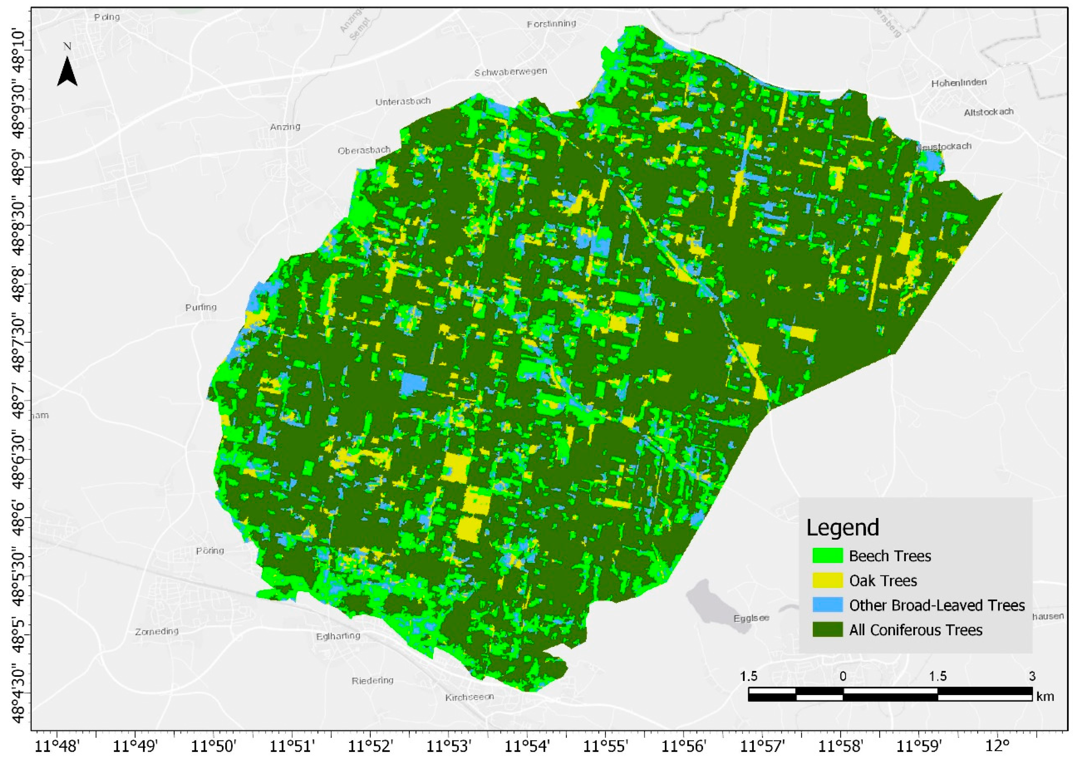
2.1. Study Area
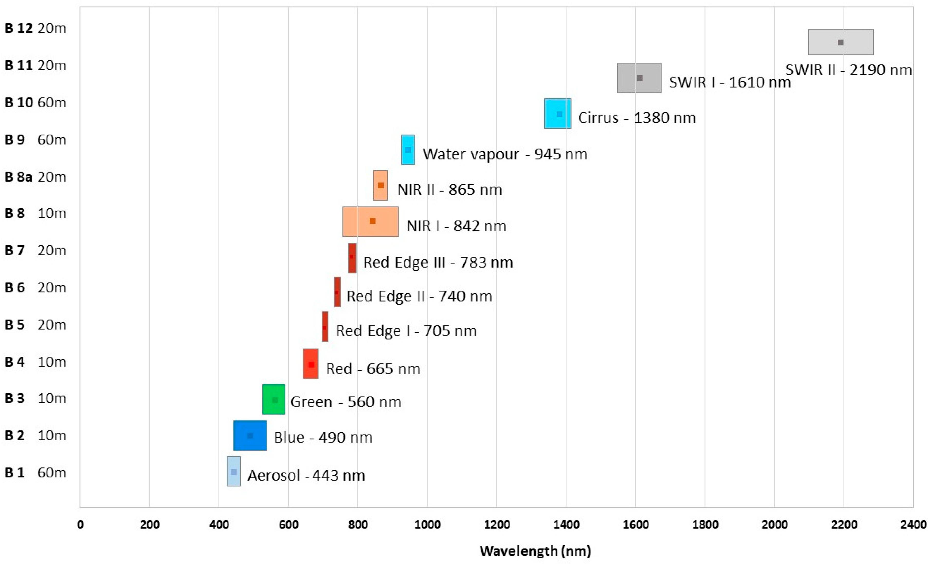
2.2. Data
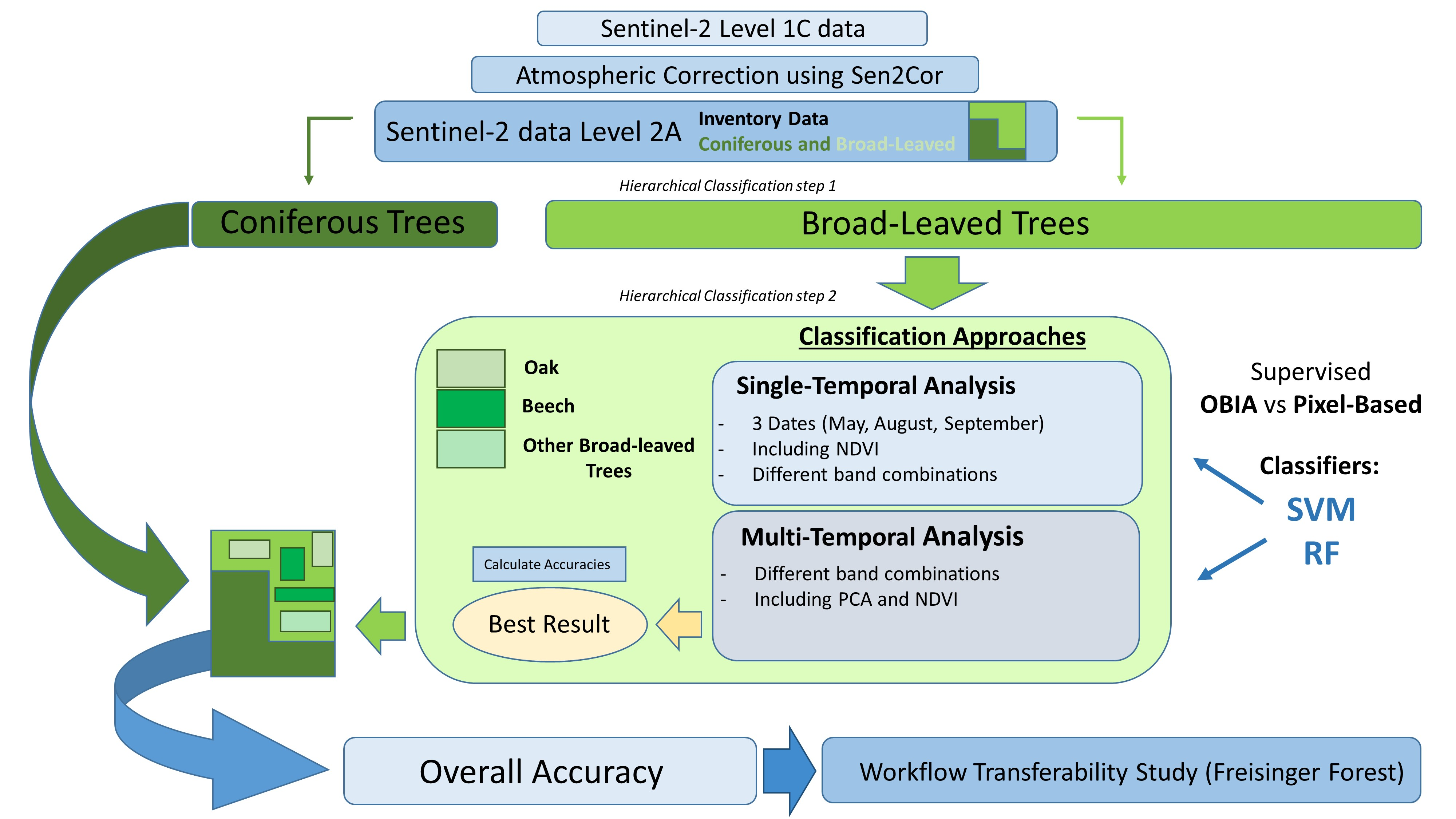
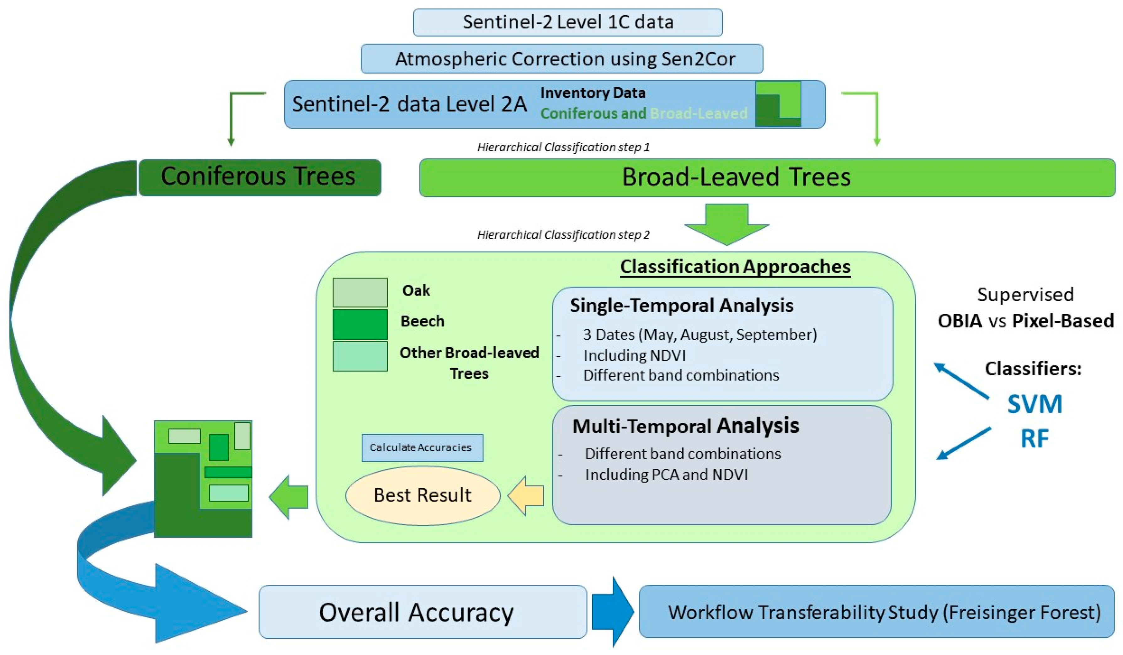
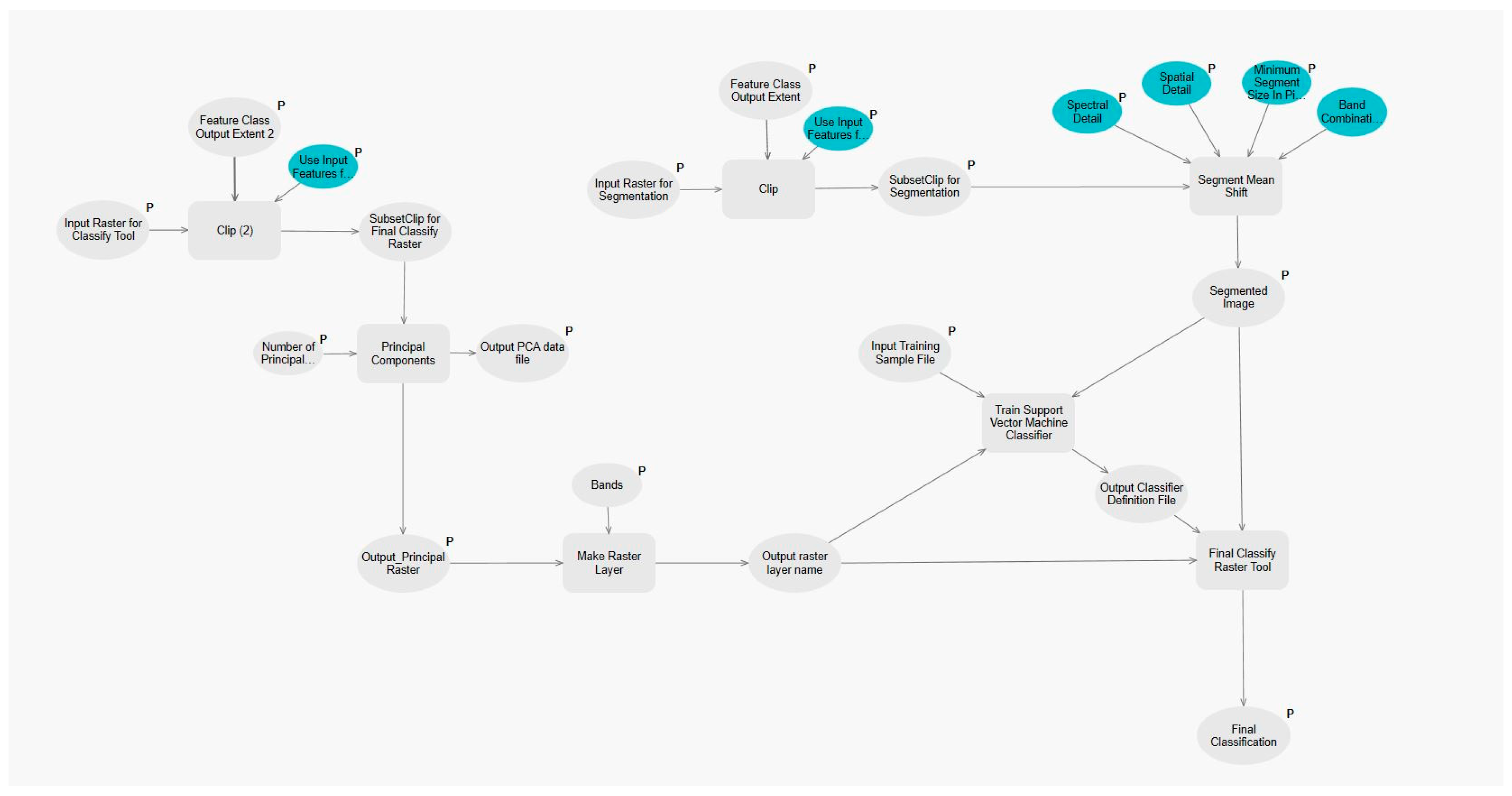
2.3. Data Pre-Processing
2.4. Classification and Accuracy Assessment
3. Results
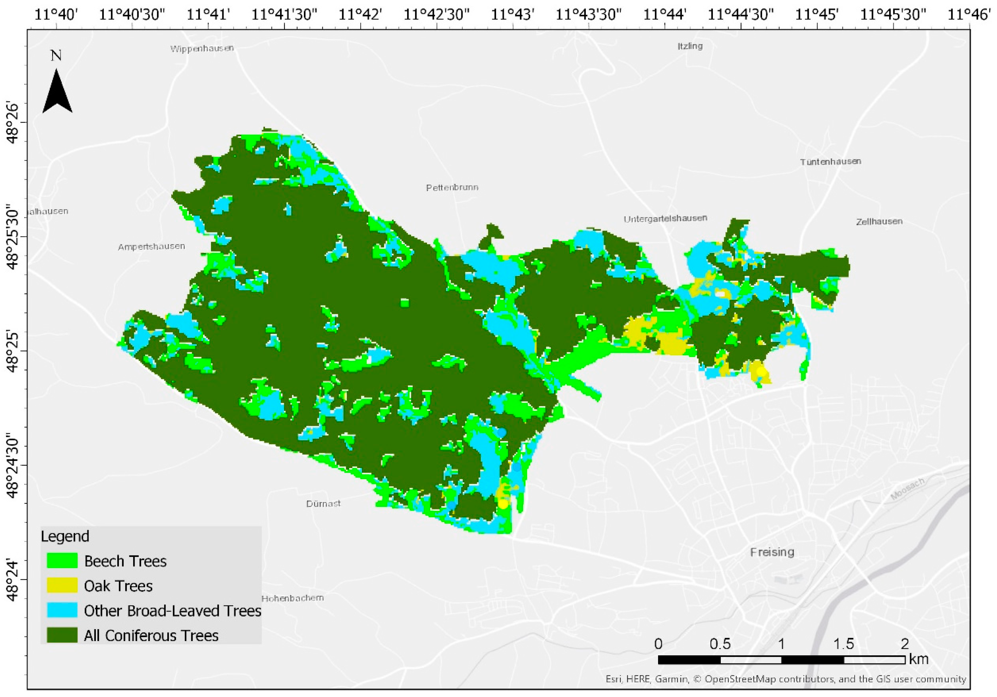
4. Transferability Study to the Freisinger Forest
5. Discussion
6. Conclusions
Author Contributions
Funding
Acknowledgments
Conflicts of Interest
References
- Dotzler, S.; Hill, J.; Buddenbaum, H.; Stoffels, J. The potential of EnMap and Sentinel-2 data for detecting drought stress phenomena in deciduous forest communities. Remote Sens. 2015, 7, 14227–14258. [Google Scholar] [CrossRef]
- Blaschke, T. Object based image analysis for remote sensing. ISPRS J. Photogram. Remote Sens. 2010, 65, 2–16. [Google Scholar] [CrossRef]
- Turner, W.; Spector, S.; Gardiner, N.; Fladeland, M.; Sterling, E.; Steininger, M. Remote sensing for biodiversity science and conservation. Trends Ecol. Evol. 2003, 18, 306–314. [Google Scholar] [CrossRef]
- Kovacs, J. Forest Cover Type Analysis of New England Forests Using Innovative WorldView-2 Imagery. Master’s Thesis, University of New Hampshire, Durham, NC, USA, 2014. [Google Scholar]
- Zhou, Y.; Qiu, F. Fusion of high spatial resolution WorldView-2 imagery and LiDAR pseudo-waveform for object-based image analysis. ISPRS J. Photogramm. Remote Sens. 2015, 101, 221–232. [Google Scholar] [CrossRef]
- Dalponte, M.; Brozzone, L.; Gianelle, D. Tree species classification in the Southern Alps based on the fusion of very high geometrical resolution multispectral/hyperspectral images and LiDAR data. Remote Sens. Environ. 2012, 123, 258–270. [Google Scholar] [CrossRef]
- Johansen, K.; Phinn, S. Mapping structural parameters and species composition of riparian vegetation using IKONOS and Landsat ETM+ data in Australian tropical savannahs. Photogramm. Eng. Remote Sens. 2006, 72, 71–80. [Google Scholar] [CrossRef]
- Peerbhay, K.Y.; Mutanga, O.; Ismail, R. Investigating the capability of few strategically placed Worldview-2 multispectral bands to discriminate forest species in KwaZulu-Natal, South Africa. IEEE J. STARS 2014, 7, 307–316. [Google Scholar] [CrossRef]
- Dennison, P.E.; Brunelle, A.R.; Carter, V.A. Assessing canopy mortality during a mountain pine beetle outbreak using GeoEye-1 high spatial resolution satellite data. Remote Sens. Environ. 2010, 114, 2431–2435. [Google Scholar] [CrossRef]
- ESA. Sentinel satellites—Overview. Observing the Earth. Available online: http://www.esa.int/Our_Activities/Observing_the_Earth/Copernicus/Overview4 (accessed on 27 December 2017).
- European Space Agency. Sentinel-2 User Handbook. Available online: https://sentinels.copernicus.eu/documents/247904/685211/Sentinel-2_User_Handbook (accessed on 27 April 2018).
- European Environment Agency. Copernicus. Available online: http://www.eea.europa.eu/about-us/what/seis-initiatives/copernicus (accessed on 28 December 2017).
- Sentinel-2 MSI Introduction. User Guides, Sentinel Online. Available online: https://sentinel.esa.int/web/sentinel/user-guides/sentinel-2-msi (accessed on 28 December 2017).
- Fassnacht, F.E.; Latifi, H.; Stereńczak, K.; Modzelewska, A.; Lefsky, M.; Waser, L.T.; Straub, C.; Ghosh, A. Review of studies on tree species classification from remotely sensed data. Remote Sens. Environ. 2016, 186, 64–87. [Google Scholar] [CrossRef]
- Immitzer, M.; Vuolo, F.; Atzberger, C. First experience with sentinel-2 data for crop and tree species classifications in central Europe. Remote Sens. 2016, 8, 166. [Google Scholar] [CrossRef]
- Ng, W.-T.; Rima, P.; Einzmann, K.; Immitzer, M.; Atzberger, C.; Eckert, S. Assessing the potential of sentinel-2 and pléiades data for the detection of prosopis and vachellia spp. In Kenya. Remote Sens. 2017, 9, 74. [Google Scholar] [CrossRef]
- Hawryło, P.; Bednarz, B.; Wężyk, P.; Szostak, M. Estimating defoliation of scots pine stands using machine learning methods and vegetation indices of Sentinel-2. Eur. J. Remote Sens. 2018, 51, 194–204. [Google Scholar] [CrossRef]
- Immitzer, M.; Böck, S.; Einzmann, K.; Vuolo, F.; Pinnel, N.; Wallner, A.; Atzberger, C. Fractional cover mapping of spruce and pine at 1 ha resolution combining very high and medium spatial resolution satellite imagery. Remote Sens. Environ. 2018, 204, 690–703. [Google Scholar] [CrossRef]
- Addabbo, P.; Focareta, M.; Marcuccio, S.; Votto, C.; Ullo, S.L. Contribution of Sentinel-2 data for applications in vegetation monitoring. Acta IMEKO 2016, 5, 44–54. [Google Scholar] [CrossRef]
- Puletti, N.; Chianucci, F.; Castaldi, C. Use of Sentinel-2 for forest classification in Mediterranean environments. Ann. Silvic. Res. 2018, 42. [Google Scholar] [CrossRef]
- Sothe, C.; Almeida, C.; Liesenberg, V.; Schimalski, M. Evaluating sentinel-2 and Landsat-8 data to map sucessional forest stages in a subtropical forest in southern brazil. Remote Sens. 2017, 9, 838. [Google Scholar] [CrossRef]
- BaySF. Regionales Naturschutzkonzept für den Forstbetrieb Wasserburg am Inn; Bayerische Staatsforsten Forstbetrieb Wasserburg: Wasserburg, Germany, 2013; p. 65. Available online: http://www.baysf.de/fileadmin/user_upload/01-ueber_uns/05-standorte/FB_Wasserburg_a._Inn/Naturschutzkonzept_Wasserburg.pdf (accessed on 8 February 2018).
- Sen2Cor. STEP, Science Toolbox Exploitation Platform. Available online: http://step.esa.int/main/third-party-plugins-2/sen2cor/ (accessed on 5 June 2017).
- Hadjimitsis, D.G.; Papadavid, G.; Agapiou, A.; Themistocleous, K.; Hadjimitsis, M.; Retalis, A.; Michaelides, S.; Chrysoulakis, N.; Toulios, L.; Clayton, C. Atmospheric correction for satellite remotely sensed data intended for agricultural applications: Impact on vegetation indices. Nat. Hazards Earth Syst. Sci. 2010, 10, 89–95. [Google Scholar] [CrossRef]
- Pal, M.; Mather, P. Support vector machines for classification in remote sensing. Int. J. Remote Sens. 2005, 26, 1007–1011. [Google Scholar] [CrossRef]
- Breiman, L. Random forests. Mach. Learn. 2001, 45, 5–32. [Google Scholar] [CrossRef]
- Pal, M. Random forest classifier for remote sensing classification. Int. J. Remote Sens. 2005, 26, 217–222. [Google Scholar] [CrossRef]
- Belgiu, M.; Drăguţ, L. Random forest in remote sensing: A review of applications and future directions. ISPRS J. Photogramm. Remote Sens. 2016, 114, 24–31. [Google Scholar] [CrossRef]
- Vapnik, V. Statistical Learning Theory; Wiley: New York, NY, USA, 1998; Volume 3. [Google Scholar]
- James, G.; Witten, D.; Hastie, T.; Tibshirani, R. An Introduction to Statistical Learning; Springer: Berlin, Germany, 2013; Volume 112. [Google Scholar]
- Yu, L.; Porwal, A.; Holden, E.-J.; Dentith, M.C. Towards automatic lithological classification from remote sensing data using support vector machines. Comput. Geosci. 2012, 45, 229–239. [Google Scholar] [CrossRef]
- ArcGIS for Desktop. Segment Mean Shift. Available online: http://desktop.arcgis.com/en/arcmap/10.3/tools/spatial-analyst-toolbox/segment-mean-shift.htm (accessed on 5 May 2017).
- Comaniciu, D.; Meer, P. Mean shift: A robust approach toward feature space analysis. IEEE Trans. Pattern Anal. Mach. Intell. 2002, 24, 603–619. [Google Scholar] [CrossRef]
- Bachofer, M.; Mayer, J. Der Kosmos Baumführer; Frankh Kosmos Verlag: Stuttgart, Germany, 2015. [Google Scholar]
- ArcMap. How Principal Components Works. Available online: http://desktop.arcgis.com/en/arcmap/10.3/tools/spatial-analyst-toolbox/how-principal-components-works.htm (accessed on 20 April 2018).
- Visa, S.; Ramsay, B.; Ralescu, A.L.; Van Der Knaap, E. Confusion matrix-based feature selection. MAICS 2011, 710, 120–127. [Google Scholar]
- Pontius, R.G., Jr.; Millones, M. Death to Kappa: Birth of quantity disagreement and allocation disagreement for accuracy assessment. Int. J. Remote Sens. 2011, 32, 4407–4429. [Google Scholar] [CrossRef]
- Ma, L.; Li, M.; Ma, X.; Cheng, L.; Du, P.; Liu, Y. A review of supervised object-based land-cover image classification. ISPRS J. Photogramm. Remote Sens. 2017, 130, 277–293. [Google Scholar] [CrossRef]
- Maldonado, S.; Weber, R. A wrapper method for feature selection using support vector machines. Inf. Sci. 2009, 179, 2208–2217. [Google Scholar] [CrossRef]
- Immitzer, M.; Atzberger, C.; Koukal, T. Tree species classification with random forest using very high spatial resolution 8-band Worldview-2 satellite data. Remote Sens. 2012, 4, 2661–2693. [Google Scholar] [CrossRef]
- Wulder, M.A.; Hall, R.J.; Coops, N.C.; Franklin, S.E. High spatial resolution remotely sensed data for ecosystem characterization. AIBS Bull. 2004, 54, 511–521. [Google Scholar] [CrossRef]
- Brandmeier, M.; Erasmi, S.; Hansen, C.; Höweling, A.; Nitzsche, K.; Ohlendorf, T.; Mamani, M.; Wörner, G. Mapping patterns of mineral alteration in volcanic terrains using aster data and field spectrometry in southern Peru. J. S. Am. Earth Sci. 2013, 48, 296–314. [Google Scholar] [CrossRef]
- Bazi, Y.; Melgani, F. Toward an optimal svm classification system for hyperspectral remote sensing images. IEEE Trans. Geosci. Remote Sens. 2006, 44, 3374–3385. [Google Scholar] [CrossRef]
- Foody, G.M.; Mathur, A. A relative evaluation of multiclass image classification by support vector machines. IEEE Trans. Geosci. Remote Sens. 2004, 42, 1335–1343. [Google Scholar] [CrossRef] [Green Version]
- Adam, E.; Mutanga, O.; Odindi, J.; Abdel-Rahman, E.M. Land-use/cover classification in a heterogeneous coastal landscape using RapidEye imagery: Evaluating the performance of random forest and support vector machines classifiers. Int. J. Remote Sens. 2014, 35, 3440–3458. [Google Scholar] [CrossRef]
- Ghosh, A.; Fassnacht, F.E.; Joshi, P.K.; Koch, B. A framework for mapping tree species combining hyperspectral and LiDAR data: Role of selected classifiers and sensor across three spatial scales. Int. J. Appl. Earth Observ. Geoinf. 2014, 26, 49–63. [Google Scholar] [CrossRef]
- Féret, J.; Asner, G.P. Tree species discrimination in tropical forests using airborne imaging spectroscopy. IEEE Trans. Geosci. Remote Sens. 2013, 51, 73–84. [Google Scholar] [CrossRef]
- Dalponte, M.; Ørka, H.O.; Ene, L.T.; Gobakken, T.; Næsset, E. Tree crown delineation and tree species classification in boreal forests using hyperspectral and ALS data. Remote Sens. Environ. 2014, 140, 306–317. [Google Scholar] [CrossRef]
- Liang, X.; Hyyppä, J.; Matikainen, L. Deciduous-coniferous tree classification using difference between first and last pulse laser signatures. Int. Arch. Photogramm. Remote Sens. Spat. Inf. Sci. 2007, 36, 253–257. [Google Scholar]
- Stratoulias, D.; Balzter, H.; Sykioti, O.; Zlinszky, A.; Tóth, V.R. Evaluating Sentinel-2 for lakeshore habitat mapping based on airborne hyperspectral data. Sensors 2015, 15, 22956–22969. [Google Scholar] [CrossRef] [PubMed]


| Date | Aquisition Time | Cloud Coverage % | Product Level |
|---|---|---|---|
| 22 May 2016 | 18:24:38 | 28.7 | 1C |
| 09 August 2016 | 05:07:27 | 4.5 | 1C |
| 29 September 2016 EF * | 18:51:41 | 0.0 | 1C |
| 29 September 2016 FF * | 18:19:08 | 0.0 | 1C |
| Tree Type | Ebersberger Forest | Freisinger Forest |
|---|---|---|
| Spruce | 777 | 70 |
| Pine | 2 | 1 |
| Larch | 6 | 2 |
| Fir | 1 | 2 |
| Other Coniferous | 8 | 2 |
| Beech | 75 | 4 |
| Oak | 21 | 2 |
| Other Broad-Leaved | 63 | 11 |
| Accuracy | Method | Classifier | Segmented Image | Segmentation Settings |
|---|---|---|---|---|
| 95.2 | OBIA | SVM | May22/Bands 6 7 8 | DS |
| 86.8 | OBIA | RF | May22/Bands 6 7 8 | DS |
| 92.3 | PB | SVM | May22/Bands 6 7 8 | DS |
| 90.2 | OBIA | SVM | May 22/Bands 3 4 8 | DS |
| 74 | OBIA | RF | May 22/Bands 3 4 8 | DS |
| 97 | PB | SVM | May 22/Bands 3 4 8 | DS |
| 87 | OBIA | SVM | May 22/Bands 3 4 8 | SegSize 5 |
| 85 | OBIA | SVM | Multitemporal/May Band 3, Aug Band 8, Sept Band 7 | DS |
| 86.6 | OBIA | RF | Multitemporal/May Band 3, Aug Band 8, Sept Band 7 | DS |
| 83 | PB | SVM | Multitemporal/May Band 3, Aug Band 8, Sept Band 7 | DS |
| 97 | OBIA | SVM | Multitemporal/May Band 8, Aug Band 8, Sept Band 8 | DS |
| 92.4 | OBIA | SVM | Multitemporal/May Band 8, Aug Band 8, Sept Band 8 | SegSize 5 |
| 81.6 | OBIA | RF | Multitemporal/May Band 8, Aug Band 8, Sept Band 8 | DS |
| 89.8 | PB | SVM | Multitemporal/May Band 8, Aug Band 8, Sept Band 8 | DS |
| Class Name | Broad-Leaved-Forest | Coniferous Forest | Total | UserAccuracy | Kappa |
|---|---|---|---|---|---|
| Broad-Leaved Forest | 35 | 0 | 35 | 1 | 0 |
| Coniferous Forest | 3 | 54 | 57 | 0.95 | 0 |
| Total | 38 | 54 | 92 | 0 | 0 |
| ProducerAccuracy | 0.92 | 1 | 0 | 0.97 | 0 |
| Kappa | 0 | 0 | 0 | 0 | 0.93 |
| Accuracy | Method | Classifier | Input Image | Segmented Additional Image | Segmentation Settings |
|---|---|---|---|---|---|
| 60.9 | OBIA | SVM | Sept 29/All Bands | May 22/Bands 8 3 2 | SegSize 5 |
| 54.3 | OBIA | SVM | Sept 29/Bands 2 3 4 5 6 7 8 9 & PCA 1-2 | May 22/Bands 8 3 2 | SegSize 5 |
| 49.4 | OBIA | SVM | Sept 29/Bands 2 3 4 5 6 7 8 9 & PCA 1-2 | May 22/Bands 8 3 2 | SegSize5 & SA 1-6 |
| 71.7 | OBIA | SVM | Sept 29/Bands 2 3 4 5 6 7 8 9 & PCA 1-4 | May 22/Bands 8 3 2 | SegSize 5 |
| 67.3 | OBIA | SVM | Sept 29/Bands 2 3 4 5 6 7 8 9 & PCA 1-5 | May 22/Bands 8 3 2 | SegSize5 & SA 1-6 |
| 59 | OBIA | SVM | Sept 29/Bands 2 3 4 5 6 7 8 9 & PCA 1-6 | May 22/Bands 8 3 2 | SegSize5 & SA 1-2-5 |
| 61.6 | OBIA | RF | Sept 29/Bands 2 3 4 5 6 7 8 9 & PCA 1-7 | May 22/Bands 8 3 2 | SegSize 5 |
| 63.3 | PB | SVM | Sept 29/Bands 2 3 4 5 6 7 8 9 & PCA 1-8 | ||
| 76.2 | PB | RF | Sept 29/Bands 2 3 4 5 6 7 8 9 & PCA 1-9 | ||
| 67.7 | OBIA | SVM | Sept 29/PCA 1-12 | May 22/Bands 8 3 2 | SegSize 5 |
| 61.8 | OBIA | SVM | May 22/All Bands | May 22/Bands 8 3 2 | SegSize 5 |
| 80.7 | OBIA | SVM | May 22/Sept 29/Bands 8 3 2 & PCA 1-4 & NDVI May 22 | May 22/Bands 8 3 2 | SegSize 5 |
| 76 | OBIA | SVM | May 22/All Bands & NDVI & PCA 1-4 | May 22/Bands 8 3 2 | SegSize 5 |
| 65 | OBIA | SVM | May 22/Bands 2 3 8 & NDVI May 22 | May 22/Bands 8 3 2 | SegSize 5 |
| 75.7 | OBIA | SVM | May 22/Bands 2 3 7 8 9 | May 22/Bands 8 3 2 | SegSize 5 |
| 74.3 | OBIA | SVM | May 22/Bands 2 3 7 8 9 & PCA 1-4 & NDVI May 22 | May 22/Bands 8 3 2 | SegSize 5 |
| 55 | PB | SVM | May 22/Bands 2 3 7 8 9 & PCA 1-4 & NDVI May 22 | ||
| 75.1 | PB | RF | May 22/Bands 2 3 7 8 9 & PCA 1-4 & NDVI May 22 | ||
| 87.2 | OBIA | SVM | May 22/Bands 5 6 7 | May 22/Bands 8 3 2 | SegSize 5 |
| 59.9 | OBIA | SVM | May 22/Bands 5 6 7 & PCA 1-4 | May 22/Bands 8 3 2 | SegSize 5 |
| 78.8 | OBIA | SVM | May 22/Bands 5 6 7 | May 22/Bands 8 3 2 | SegSize5 & SA 1-2-3-4 |
| 53.7 | PB | SVM | May 22/Bands 5 6 7 | ||
| 67.1 | OBIA | RF | May 22/Bands 5 6 7 | May 22/Bands 8 3 2 | SegSize 5 |
| 87.2 | OBIA | SVM | May 22/Bands 5 6 7 & NDVI May 22 | May 22/Bands 8 3 2 | SegSize 5 |
| 87.2 | OBIA | SVM | May 22/Bands 4 5 6 7 | May 22/Bands 8 3 2 | SegSize 5 |
| 62.5 | OBIA | RF | May 22/Bands 4 5 6 7 | May 22/Bands 8 3 2 | SegSize 5 |
| 80.3 | OBIA | SVM | May 22/Band 7 & Aug 09/Band 6 & May 22/Band 5 | May 22/Bands 8 3 2 | SegSize 5 |
| 63.3 | OBIA | SVM | May 22/PCA 1-12 | May 22/Bands 8 3 2 | SegSize 5 |
| 60 | OBIA | SVM | May 22/All Bands & PCA May 1-4 | May 22/Bands 8 3 2 | SegSize 5 |
| 89.1 | OBIA | SVM | August 09/All Bands | May 22/Bands 8 3 2 | SegSize 5 |
| 63.1 | OBIA | RF | August 09/All Bands | May 22/Bands 8 3 2 | SegSize 5 |
| 46 | PB | SVM | August 09/All Bands | ||
| 65.2 | OBIA | SVM | August 09/All Bands & PCA May 1-4 | May 22/Bands 8 3 2 | SegSize 5 |
| 80.5 | OBIA | SVM | August 09/Bands 5 6 7 | May 22/Bands 8 3 2 | SegSize 5 |
| 80.7 | OBIA | SVM | August 09/Bands 2 3 8 | May 22/Bands 8 3 2 | SegSize 5 |
| 91 | OBIA | SVM | August 09/PCA 1-12 | May 22/Bands 8 3 2 | SegSize 5 |
| 78.3 | OBIA | SVM | August 09/PCA 1-3 | May 22/Bands 8 3 2 | SegSize 5 |
| 86.3 | OBIA | SVM | August 09/PCA 1-4 | May 22/Bands 8 3 2 | SegSize 5 |
| 53.3 | OBIA | RF | August 09/PCA 1-4 | May 22/Bands 8 3 2 | SegSize 5 |
| 51 | PB | SVM | August 09/PCA 1-10 | ||
| 90.5 | OBIA | SVM | August 09/PCA 1-5 | May 22/Bands 8 3 2 | SegSize 5 |
| 84.5 | OBIA | SVM | August 09/PCA 1-6 | May 22/Bands 8 3 2 | SegSize 5 |
| 85.2 | OBIA | SVM | August 09/PCA 1-7 | May 22/Bands 8 3 2 | SegSize 5 |
| 80.8 | OBIA | SVM | August 09/PCA 1-10 | May 22/Bands 8 3 2 | SegSize 5 |
| 81.9 | OBIA | SVM | August 09/PCA 1-11 | May 22/Bands 8 3 2 | SegSize 5 |
| 90.9 | OBIA | SVM | August 09/PCA 1-12 | May 22/Bands 8 3 2 | SegSize 5 |
| 72.3 | OBIA | SVM | August 09/PCA 1 & 4 | May 22/Bands 8 3 2 | SegSize 5 |
| 74.8 | OBIA | SVM | August 09/PCA 2-4 | May 22/Bands 8 3 2 | SegSize 5 |
| 78.3 | OBIA | SVM | August 09/PCA 1 | May 22/Bands 8 3 2 | SegSize 5 |
| 80.8 | OBIA | SVM | August 09/NDVI August | May 22/Bands 8 3 2 | SegSize 5 |
| 73.5 | OBIA | SVM | August 09/PCA 1-12 & NDVI August 09 | May 22/Bands 8 3 2 | SegSize 5 |
| 77.2 | OBIA | SVM | August 09/PCA All & Sept 29/PCA All | May 22/Bands 8 3 2 | SegSize 5 |
| 66 | OBIA | SVM | May 22/PCA All & August 09/PCA 1-12 & Sept 29/PCA 1-12 | May 22/Bands 8 3 2 | SegSize 5 |
| 82.3 | OBIA | SVM | May 22/PCA All & August 09/PCA All | May 22/Bands 8 3 2 | SegSize 5 |
| Class Name | Beech Trees | Oak Trees | Other Broad-Leaved | Total | UserAccuracy | Kappa |
|---|---|---|---|---|---|---|
| Beech Trees | 15 | 0 | 1 | 16 | 0.94 | 0 |
| Oak Trees | 0 | 21 | 0 | 21 | 1 | 0 |
| Other Broad-Leaved | 4 | 0 | 17 | 21 | 0.81 | 0 |
| Total | 19 | 21 | 18 | 58 | 0 | 0 |
| ProducerAccuracy | 0.79 | 1 | 0.94 | 0 | 0.91 | 0 |
| Kappa | 0 | 0 | 0 | 0 | 0 | 0.87 |
| Class Name | Beech Trees | Oak Trees | Other Broad-Leaved | Coniferous Forest | Total | UserAccuracy | Kappa |
|---|---|---|---|---|---|---|---|
| Beech Trees | 15 | 0 | 1 | 0 | 16 | 0.94 | 0 |
| Oak Trees | 0 | 21 | 0 | 0 | 21 | 1 | 0 |
| Other Broad-Leaved | 4 | 0 | 17 | 0 | 21 | 0.81 | 0 |
| Coniferous Forest | 2 | 0 | 3 | 20 | 25 | 0.8 | 0 |
| Total | 21 | 21 | 21 | 20 | 83 | 0 | 0 |
| ProducerAccuracy | 0.71 | 1 | 0.81 | 1 | 0 | 0.88 | 0 |
| Kappa | 0 | 0 | 0 | 0 | 0 | 0 | 0.83 |
| Class Name | Beech Trees | Oak Trees | Other Broad-Leaved | Coniferous Forest | Total | UserAccuracy | Kappa |
|---|---|---|---|---|---|---|---|
| Beech Trees | 5 | 3 | 1 | 0 | 9 | 0.56 | 0 |
| Oak Trees | 0 | 11 | 0 | 0 | 11 | 1 | 0 |
| Other Broad-Leaved | 2 | 0 | 6 | 0 | 8 | 0.75 | 0 |
| Coniferous Forest | 0 | 0 | 0 | 11 | 11 | 1 | 0 |
| Total | 7 | 14 | 7 | 11 | 39 | 0 | 0 |
| ProducerAccuracy | 0.71 | 0.79 | 0.86 | 1 | 0 | 0.85 | 0 |
| Kappa | 0 | 0 | 0 | 0 | 0 | 0 | 0.79 |
© 2018 by the authors. Licensee MDPI, Basel, Switzerland. This article is an open access article distributed under the terms and conditions of the Creative Commons Attribution (CC BY) license (http://creativecommons.org/licenses/by/4.0/).
Share and Cite
Wessel, M.; Brandmeier, M.; Tiede, D. Evaluation of Different Machine Learning Algorithms for Scalable Classification of Tree Types and Tree Species Based on Sentinel-2 Data. Remote Sens. 2018, 10, 1419. https://0-doi-org.brum.beds.ac.uk/10.3390/rs10091419
Wessel M, Brandmeier M, Tiede D. Evaluation of Different Machine Learning Algorithms for Scalable Classification of Tree Types and Tree Species Based on Sentinel-2 Data. Remote Sensing. 2018; 10(9):1419. https://0-doi-org.brum.beds.ac.uk/10.3390/rs10091419
Chicago/Turabian StyleWessel, Mathias, Melanie Brandmeier, and Dirk Tiede. 2018. "Evaluation of Different Machine Learning Algorithms for Scalable Classification of Tree Types and Tree Species Based on Sentinel-2 Data" Remote Sensing 10, no. 9: 1419. https://0-doi-org.brum.beds.ac.uk/10.3390/rs10091419