Using APAR to Predict Aboveground Plant Productivity in Semi-Arid Rangelands: Spatial and Temporal Relationships Differ

Abstract

Monitoring of aboveground net primary production (ANPP) is critical for effective management of rangeland ecosystems but is problematic due to the vast extent of rangelands globally, and the high costs of ground-based measurements. Remote sensing of absorbed photosynthetically active radiation (APAR) can be used to predict ANPP, potentially offering an alternative means of quantifying ANPP at both high temporal and spatial resolution across broad spatial extents. The relationship between ANPP and APAR has often been quantified based on either spatial variation across a broad region or temporal variation at a location over time, but rarely both. Here we assess: (i) if the relationship between ANPP and APAR is consistent when evaluated across time and space; (ii) potential factors driving differences between temporal versus spatial models, and (iii) the magnitude of potential errors relating to space for time transformations in quantifying productivity. Using two complimentary ANPP datasets and remotely sensed data derived from MODIS and a Landsat/MODIS fusion data product, we find that slopes of spatial models are generally greater than slopes of temporal models. The abundance of plant species with different structural attributes, specifically the abundance of C4 shortgrasses with prostrate canopies versus taller, more productive C3 species with more vertically complex canopies, tended to vary more dramatically in space than over time. This difference in spatial versus temporal variation in these key plant functional groups appears to be the primary driver of differences in slopes among regression models. While the individual models revealed strong relationships between ANPP to APAR, the use of temporal models to predict variation in space (or vice versa) can increase error in remotely sensed predictions of ANPP.

1. Introduction

Monitoring of plant phenology and aboveground net primary production (ANPP) is critical for effective management of grassland and rangeland ecosystems, particularly for managers seeking to flexibly match forage demand of livestock with forage availability [1,2]. However, accurate measurements of spatial and temporal variability in ANPP at scales relevant to rangeland managers is challenging due the substantial labor costs associated with directly harvesting biomass with sufficient replication across the vast areas of the earth managed for livestock production. Satellite-based remote sensing has been hailed as a solution to this challenge because of the well-known positive relationship between the Normalized Difference Vegetation Index (NDVI) and the proportion of incoming photosynthetic active radiation (fPAR) absorbed by active growing vegetation [3,4,5]. This relationship has led to numerous analyses of relationships between NDVI or, more recently the Enhanced Vegetation Index [4], and ANPP on all the vegetated continents [6,7,8,9,10,11]. Although spectral indices may be ineffective in estimating ANPP where leaf area and seasonal patterns of carbon gain are not highly correlated, such as in evergreen vegetation [12,13], the seasonal development of the canopy and accumulation of carbon are closely coupled in grass-dominated ecosystems, making them a promising candidate for the use of NDVI to remotely estimate ANPP [6].

Approaches for relating NDVI to ANPP typically rely on a season-long integration of NDVI values from frequently repeated measurements of a location over time (iNDVI), such as from the Advanced Very High Resolution Radiometer/National Oceanic and Atmospheric Agency (AVHRR/NOAA) available at a 1-km resolution [6], or the Moderate Resolution Imaging Spectroradiometer (MODIS) available at a 250–1000-m resolutions [4,14]. Studies using these satellite platforms have demonstrated clear relationships between iNDVI and ANPP based on regression models describing spatial variation among locations that span a broad gradient in ANPP (e.g., across the rainfall gradients in grasslands of North and South America [6,7,8,9,14]), or models examining temporal variation either within the growing season [8,14] or among years for a given locality, where the size of a locality varies from a single pixel [15] to several square kilometers [16]. Two limitations to these approaches are (1) uncertainty regarding the equivalence of spatial versus temporal regression models, and (2) the coarse resolution of the ANPP estimation in existing spatial regression models, which limits utility for rangeland managers [17]. Landsat imagery measures NDVI at a finer spatial resolution (e.g., 30 m) and can effectively monitor long-term changes in peak plant greenness or biomass at a given locality, thereby allowing managers to monitor trends in rangeland conditions [18]. However, Landsat imagery is available at less frequent intervals, such that temporal changes in NDVI over a growing season are more difficult to accurately measure, particularly when a portion of the images during the growing season include cloud cover [19]. Furthermore, Landsat scenes collected at different times within the growing season can produce different slopes for the relationship of spectral indices to ANPP [19]. Within a scene, spatial variation in greenness can be quantified relative to reference sites [20], but generating absolute values of ANPP in known units requires site and scene-specific calibration.

Spatial variability in plant community composition introduces another key challenge to broad-scale remote sensing of ANPP. Slopes for regression models relating iNDVI (or iAPAR derived from iNDVI and PAR) to ANPP can vary substantially among vegetation types. For example, Grigera et al. [14] found the slope for sown upland pastures was more than double that for naturalized lowland pastures in South America. In extensive rangeland systems with diverse native plant communities, a key uncertainty is the degree to which relationships between iNDVI and ANPP change in response to more subtle shifts in the relative abundance of different forage species associated with changes in soils, topography, climate, or the history of grazing management. The extent to which changes in plant community composition alter the slope of the NDVI-ANPP relationship will determine how extensively landscapes need to be stratified or subdivided into units that each require their own calibration. In landscapes where a small number of communities adequately characterize such variation (e.g., the two types of pastures modelled by Grigera et al. 2007 [14]), remote sensing of ANPP can be a powerful resource for rangeland managers. Such utility will be restricted in landscapes where plant community compositional heterogeneity results in a large number of strata that each require their own calibration.

Here, we examined relationships between remotely sensed measurements of NDVI at two spatial scales (250-m and 30-m pixels) and ground-based measurements of ANPP at two corresponding spatial scales (130-ha pastures and 3-ha plots) within a 6500 ha experimental ranch in the shortgrass steppe of eastern Colorado, USA. NDVI was converted to an estimate of APAR following the approach of Grigera et al. [14], and relationships between ANPP and integrated APAR (iAPAR) were examined both in terms of spatial variation within a year, and temporal variation among years, at both spatial scales. The relationship was first examined using a long-term grazing management experiment (in place since 1939) which has altered grassland species composition in well-documented ways across relatively homogenous underlying soil characteristics [21,22,23]. We then examine spatial and temporal variation in ANPP across pastures where prior grazing management has been consistent historically, but vegetation varies due to heterogeneity in soil types, topography, and locally variable rainfall. In this latter experiment, to obtain measurements of NDVI at both a high spatial (30 m) and temporal (daily) resolution, we used a data fusion approach that integrates surface reflectance from MODIS and Landsat platforms to generate a daily NDVI time series over the growing season for each 30-m pixel. These datasets were used to examine the consistency of the ANPP-iAPAR relationship in space and in time, and discuss the implications for remote sensing of ANPP at fine spatial resolution over broad spatial extents.

2. Materials and Methods

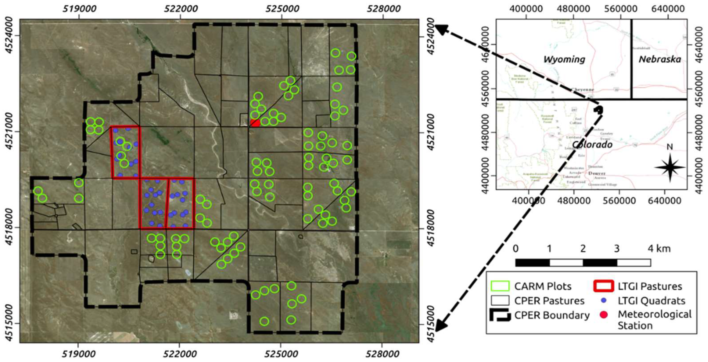
2.1. Study Area

This research was conducted at the USDA ARS Central Plains Experimental Range (CPER), a Long-Term Agroecosystem Research site located in northeastern Colorado (40°49’N, 107°46’W; Figure 1). The study area is dominated by shortgrass steppe vegetation, with a mix of perennial warm-season (C4) and cool-season (C3) graminoids. Blue grama (Bouteloua gracilis [Willd. ex Kunth] Lag. ex Griffiths) is the dominant warm season grass species, with buffalograss (B. dactyloides [Nutt.] J.T. Columbus) and plains pricklypear cactus (Opuntia polyacantha Haw.) as subdominants. Dominant perennial cool-season graminoids included needle-and-thread (Hesperostipa comata [Trin. & Rupr.] Barkworth), needle-leaf sedge (Carex duriuscula C.A. Mey.), and western wheatgrass (Pascopyrum smithii [Rydb.] Á. Löve). The dominant forb and subshrub are Scarlet globemallow (Sphaeralcea coccinea [Nutt.] Rydb.), and fringed sagewort (Artemisia frigida Willd.), respectively. Annual grasses consist almost entirely of six-weeks fescue (Vulpia octoflora [Walter] Rydb.). The mean annual precipitation is 34 cm and the mean annual temperature is 8.4 ℃, ranging from −2.6 ℃ in December to 21.3 ℃ in July.

2.2. Ground Based Observations

Ground-based estimates of ANPP were compiled from two independent experiments at the CPER: the Long-Term Grazing Intensity (LTGI) experiment and the Collaborative Adaptive Rangeland Management (CARM) experiment. Starting in 1939, the Long-Term Grazing Experiment [23,24] has consistently applied three distinct cattle grazing intensities, light (20% utilization of peak growing season biomass), moderate (40% utilization), and heavy (60% utilization), from mid-May to October with season-long grazing on three adjoining ~130 hectare pastures (Figure 1). The three experimental pastures have a uniform soil type (loamy) and are topographically similar. ANPP was measured from 2003–2016 in the last week of July or the first week of August, corresponding to the historical timing of peak biomass. For ANPP measurements, twelve 1.5 m² temporary exclosures were established each year and co-located with 4 permanent transects (3 exclosures per transect) in each pasture. Each spring, the 3 exclosures associated with a transect were moved in a random distance and cardinal direction. ANPP was measured in 0.1 m² quadrats within each exclosure by clipping all aboveground biomass at ground level. Shrubs and cacti were excluded from ANPP measurements due to the inability of the sampling procedure to characterize the extreme spatial variability of these plants, which on average, account for less than 5% of the total biomass. Clipped biomass was separated into seven plant functional groups: perennial C3 cool-season graminoids (C3PG), Bouteloua spp. (BOBU), other perennial C4 warm-season grasses (OC4PG), annual grasses (AG), forbs (FORBS), subshrubs, and standing dead vegetation. Aboveground net herbaceous productivity (ANHP) was calculated by summing biomass of all these functional groups except subshrubs and standing dead. Subshrubs are an extremely minor component of ANPP, but including them in ground-based measurements can increase variance in ANPP estimates, hence they were excluded. Hereafter, we use the term ANHP to denote our best estimate of ANPP.

The Collaborative Adaptive Rangeland Management (CARM) experiment [25] contrasts the impacts of traditional versus adaptive grazing management practices. The study contains twenty, ~130-ha pastures, 10 of which are adaptively managed with rotational grazing of one large herd of cattle while 10 pastures are traditionally managed with moderate levels of continuous season-long grazing. All pastures are grazed from mid-May to October. For the first pre-treatment year of the experiment (2013), all 20 pastures were managed in a similar manner with a moderate stocking rate and continuous season-long grazing. In subsequent years, the adaptively managed pastures were excluded from our remote sensing analyses to ensure that we are examining spatial variation in ANHP across pastures with consistent grazing management (i.e., we used only the traditionally managed pastures, N = 10). Each pasture in the CARM experiment contains four to six 125-m radius plots that include four 30-m transects in each quadrant (Figure 1 and Figure 2). Of the four transects per plot, two are used to measure ANHP by clipping biomass inside temporary grazing exclosures located at 10 m and 20 m along each transect. Methods to determine ANHP were the same as those described for the LTGI study above, except we clipped biomass from a 0.18 m² quadrat in each temporary exclosure. The CARM biomass is sampled within a few days after the LTGI pastures are clipped. Similar to the LTGI study, each spring the CARM exclosures are moved in a random distance and cardinal direction around each transect.

While the LTGI and CARM experiments are co-located at the same study area, they apply two very different conceptual study designs. The LTGI experiment involves three non-replicated pastures, each with a different long-term grazing history, but soil type and topography are similar across the three pastures. The ground-based sampling scheme for LTGI is specifically designed to assess annual variation in vegetation dynamics at the pasture scale. The CARM experiment involves pastures with varying soil types (encompassing a gradient from loamy to sandy soil texture; see [22]), but consistent grazing management. While the overall scale of the CARM experiment is larger (more pastures, plots, and samples), the sampling protocol does not characterize individual pasture dynamics as accurately as the LTGI experiment. Therefore, it is useful to conceptualize the LTGI experiment as characterizing pasture scale vegetation dynamics and the CARM experiment as characterizing plot scale vegetation dynamics. Simply due to their differing spatial scales, the CARM measurements encompass a broader range in the magnitude of ANHP and plant functional group biomass across a more diverse landscape than the LTGI pasture-scale study.

A meteorological station located at CPER measured hourly incoming photosynthetically active radiation (PAR) (Figure 1). PAR measurements were aggregated at a daily time step and subsequently used in the calculation of the absorbed photosynthetically active radiation (APAR) time series.

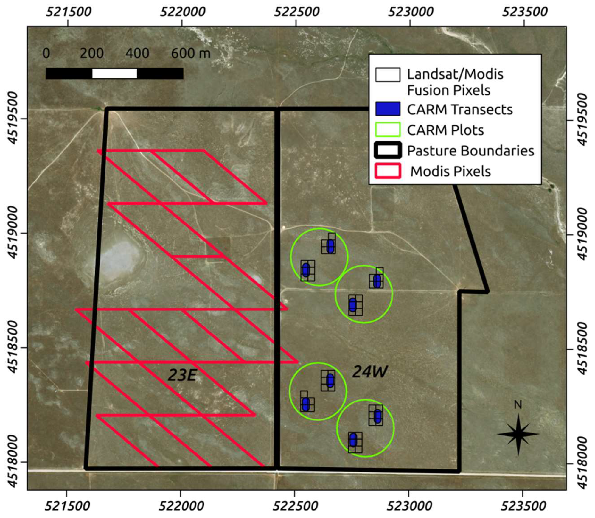
2.3. Remotely Sensed Observations and Aggregations

NDVI observations from the Terra and Aqua MODIS satellites were used to develop time series across the study area. The MOD13Q1 V006 [26] and MYD13Q1 V006 [27] are each a composite dataset that select the best pixel value over a 16-day interval, and, when combined, result in a quasi 8-day time series. The two MODIS datasets were aggregated and downloaded from Google Earth Engine [28] for the study area. The resulting data had a nominal spatial resolution of 250-m at a quasi 8-day interval. Using the pixel reliability metric band, observations that were deemed less than marginal were discarded. The resulting 8-day NDVI time series data was linearly interpolated to daily data for each pixel. The spatial and temporal scales of the resulting data (termed NDVI₂₅₀), was sufficient to characterize the spatial and temporal dynamics at the LTGI pasture scale. To avoid edge effects when aggregating the NDVI₂₅₀ time series to the LTGI pastures, pixels with less than 90% overlap with a pasture, excluding existing exclosures and the playa located between the light and heavy pastures, were excluded (Figure 1). The remaining data were spatially averaged to produce a pasture specific daily time series. The resulting NDVI to LTGI ANHP characterization included a total of 12 in-situ measurements of peak ANHP per pasture and 13, 11, and 14 MODIS pixels in the light, moderate, and heavily grazed pastures, respectively.

A major challenge for remote sensing of rangelands at scales relevant to managers is quantifying spatial patterns at sufficiently fine spatial resolutions. A remote sensing data fusion technique was used to integrate the spatial resolution of Landsat imagery with the temporal resolution of MODIS imagery. The Spatial and Temporal Adaptive Reflectance Fusion Model (STARFM) [29,30] was used to generate a Landsat-MODIS data fusion product. The STARFM approach blends Landsat (30-m spatial and 16-day temporal resolution) and MODIS (250-m spatial and 1-day temporal resolution) surface reflectance. The MODIS daily bi-directional surface reflectance (MOD09GQ) was first corrected to the nadir view reflectance using MODIS BRDF product (MCD43A1). The resulting 30-m spatial and daily temporal resolution surface reflectance dataset was used to compute NDVI (termed NDVI₃₀). Daily NDVI images may still have gaps due to cloud interference in either Landsat or MODIS images. To make a complete time-series NDVI, we used the Savitzky–Golay (SG) filter to smooth data and fill gaps. The SG filter is a moving fitting approach. Each point is smoothed using the value computed from the polynomial function fit to the observations within the moving window. Both original Landsat and the fused Landsat-MODIS data were used in this process. The resulting daily NDVI time series at 30-m resolution was able to characterize NDVI dynamics at appropriate scales for comparison to the ground-based CARM biomass observations (Figure 2). This is the first time we have been able to investigate the relationships between ANHP and NDVI or iAPAR for rangelands using daily observations at 30-m resolution through multi-sensor data fusion.

The CARM biomass data were aggregated at the plot level with mean and variance calculated for each set of quadrats (N = 4). For the NDVI₃₀ data, we calculated the mean value for all pixels within a 15-m buffer around each 30-m transect. The mean NDVI value per transect was calculated with bilinear resampling, and then the values from the two transects were averaged for each plot.

The in situ and remotely sensed data associated with the CARM and LTGI studies are complementary. The LTGI data strongly characterize the temporal relationship (N = 14 years) with few replicates (N = 3 pastures) and poorly characterize the spatial relationship (N = 3 pastures) with many replicates (N = 14 years). In contrast, the CARM data strongly characterize the spatial relationship (N = 40 to 92 plots depending on year) with few temporal replicates (N = 4 years) and poorly characterize the temporal relationship (N = 4 years) with many replicates (N = 46 plots that were measured in ≥3 years). These differing but complementary datasets allowed us to assess how variation in time, space, and plant community composition affect the ANHP-iAPAR relationship.

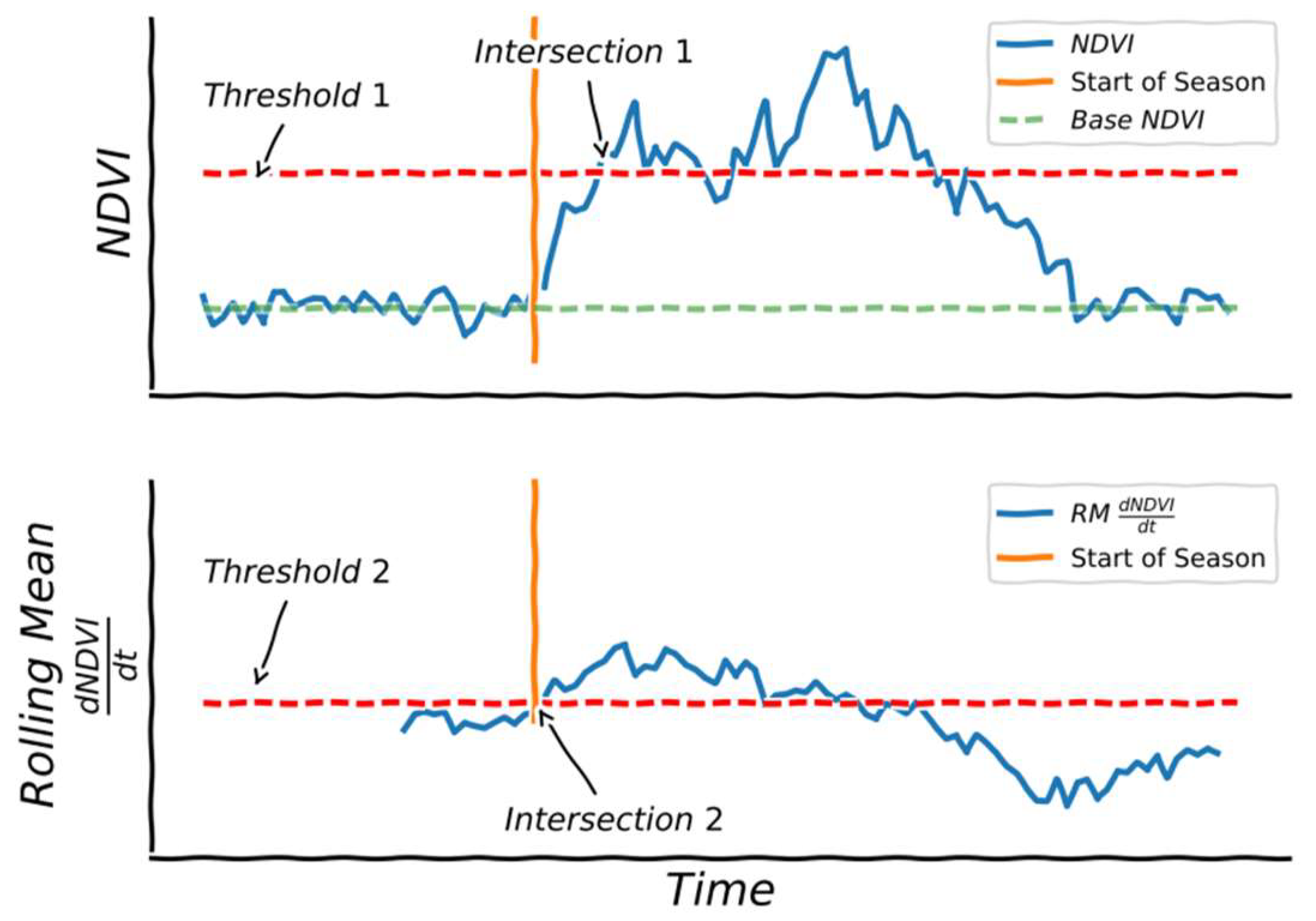
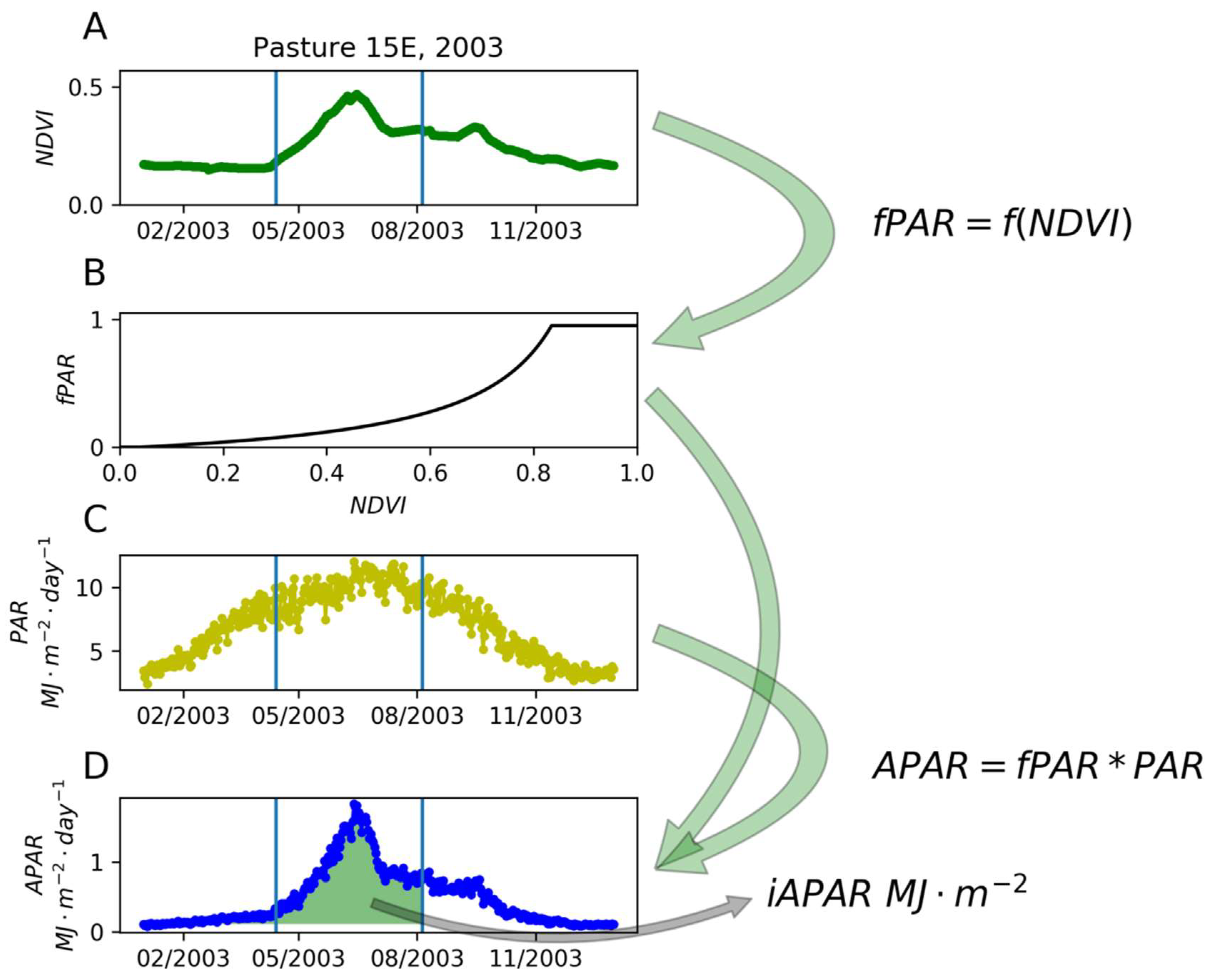
2.4. Phenological Calculations

To infer the total live biomass for a growing season from remotely sensed data, a “start of the growing season” phenologic metric was calculated from the NDVI time series (Figure 3). We used a two staged threshold approach to calculate the start of the growing season. The first threshold was set to the first date the NDVI time series reached the 30th (LTGI) or 50th (CARM) percentile (Figure 3, a schematic generated from non-real data). The percentiles for the first threshold were calculated from the NDVI data between 1 April; 19 July. Starting from the date the first threshold intersected the NDVI time series, the algorithm worked backwards until the second threshold was intersected. The second threshold was the 40th (LTGI) or 30th (CARM) percentile of the 25 day rolling average of the differenced NDVI time series.

To estimate APAR, the time series of NDVI was converted to fPAR following methods by Grigera et al. and Caride et al. [14,31] using an exponential function between fPAR and NDVI. To do so, we used the parameters proposed in Grigera et al. [14] derived from vegetation with a similar structure and herbaceous species. The fPAR time series is multiplied with PAR measured at the CPER meteorological station to calculate the APAR time series (Equation (1), Figure 4).

The APAR and NDVI values associated with the dormant period were calculated annually as the average APAR/NDVI between the first (non-interpolated) NDVI observation of that year and 16 March (denoted as base APAR or NDVI). Cumulative APAR (iAPAR) is calculated by numerically integrating from the start of the season to the quadrat clip date and between the base APAR value and the APAR time series (Equation (1), Figure 4). Including the base APAR value in the iAPAR calculation minimizes any error in the start of the growing season calculation and reduces the effect of spatially heterogeneous soils on the observed NDVI.

$$iAPAR={{\displaystyle \int }}_{t=start\_of\_season}^{t=clip\_date}(fPAR\left(NDV{I}_t\right)\ast PA{R}_t-APA{R}_{base})dt$$

(1)

An example of the iAPAR calculation is shown in Figure 4 (see Supplemantary Materials for all phenologic calculations). Based on visual inspection, the start of the growing season calculation and the region of integration were accurate for all the NDVI/APAR time series in the study. The mean and standard deviation of the start of the season metric for each year ranged from 96 to 144 and 0 to 5 days for the LTGI pastures and from 94 to 118 and 6 to 12 days for the CARM plots, respectively. The difference in the range of the start of season between the LTGI (14 years) and CARM (4 years) study is due to the greater temporal variability in the start of the season metric as compared to the spatial variability.

2.5. Statistical Approaches

We fit linear regression models relating ANHP to iAPAR for each set of spatial and temporal collections from the CARM and LTGI studies independently. Slopes from the ANHP to iAPAR relationships are related to the radiation use efficiency (RUE), a measure of a plant community’s ability to convert incoming PAR to dry plant matter. In cases where the Y-intercept equals zero the slope coefficient is equivalent to the RUE. Non-zero Y-intercepts suggest an increasing (negative Y-intercept) or decreasing (positive Y-intercept) RUE efficiency across the range of iAPAR values [32]. We compared slopes from temporal and spatial models for each study using t-tests. For LTGI data, which were normally-distributed, we used a parametric t-test assuming unequal variances to compare slopes from temporal vs. spatial models. Slopes were square-root transformed to attain normally distributed model residuals. For CARM data and for all data combined, which were not normally-distributed, we used two-sample Wilcoxon nonparametric tests to compare slopes from temporal vs. spatial models. Models with R² less than 0.1 (N = 5) were excluded from statistical analyses. For LTGI data, to determine how long-term grazing management affected the temporal relationship between ANHP and iAPAR, we ran an ANOVA with grazing intensity (light, moderate, heavy), iAPAR, and the interaction between these two terms as predictors, and ANHP as the response variable. Residuals were checked for normality and homogeneity of variances. This analysis approach was not applicable to CARM data because all pastures included in the CARM dataset experienced the same grazing treatment (moderate season-long grazing).

We used multiple linear regression to assess how plant functional groups affected the relationship between ANHP and iAPAR. Specifically, we modeled iAPAR (response variable) as a function of aboveground biomass of all functional groups (predictor variables). Standing dead biomass was excluded in the ANHP aggregation but included in these functional group regressions to test if it would impact the predicted iAPAR and therefore the relationship between ANHP and iAPAR. Due to the wide range in variance within the biomass data, we used inverse variance weighting of the total ANHP by pasture (LTGI) or plot (CARM) when fitting the models. This approach gave more weight to observations for which we had higher confidence. For the CARM data, due to the hierarchical study design in which each pasture contained multiple plots, we implemented a mixed effects linear model with pasture as a random intercept to account for autocorrelation among plots within the same pasture. For this analysis we used a linear and nonlinear mixed effects model package in R [33]. For the LTGI data for which data were already aggregated at the scale of pasture, we used the base R linear model function [34]. For the LTGI model, we transformed iAPAR by exponentiation to the 1.5 power to attain normally-distributed model residuals.

3. Results

We found strong positive correlations between ANHP and iAPAR in the CARM (NDVI₃₀) and LTGI (NDVI₂₅₀) data for both temporal and spatial models (Figure 5 and

Table 1. Model results from the spatial and temporal linear regressions of ANHP on iAPAR for the LTGI and CARM experiments. In the “Type” column, sp = spatial model and temp = temporal model. The “Model” column refers to the year (for spatial models) or pasture/plot for temporal models.

Model	R2	Slope	Intercept	Type	Dataset		Model	R2	Slope	Intercept	Type	Dataset		Model	R2	Slope	Intercept	Type	Dataset
2003	0.76	0.70	48.75	sp	LTGI		15E P3	0.01	−0.07	80.14	temp	CARM		25SE P1	0.50	1.14	19.17	temp	CARM
2004	1.00	2.76	−33.96	sp	LTGI		15E P4	0.01	−0.03	93.45	temp	CARM		25SE P2	0.94	2.01	−38.79	temp	CARM
2005	0.95	3.01	−170.62	sp	LTGI		17N P1	0.34	3.39	−100.82	temp	CARM		25SE P3	0.81	1.56	7.58	temp	CARM
2006	1.00	4.23	−149.40	sp	LTGI		17N P2	0.68	1.50	−9.24	temp	CARM		25SE P4	0.81	0.92	29.02	temp	CARM
2007	0.98	2.73	−66.00	sp	LTGI		17N P3	0.69	1.78	45.12	temp	CARM		26E P1	0.87	2.03	−41.87	temp	CARM
2008	0.14	1.64	−13.53	sp	LTGI		17N P4	1.00	2.08	0.50	temp	CARM		26E P2	0.94	1.29	−12.66	temp	CARM
2009	0.98	5.98	−505.20	sp	LTGI		17N P5	0.47	1.12	13.27	temp	CARM		26E P3	1.00	1.27	−3.34	temp	CARM
2010	1.00	10.34	−769.89	sp	LTGI		17N P6	0.91	2.17	−39.75	temp	CARM		26E P4	0.43	1.77	−33.68	temp	CARM
2011	0.91	2.00	−35.98	sp	LTGI		19N P1	0.73	1.48	38.26	temp	CARM		31E P1	0.60	1.28	−4.22	temp	CARM
2012	0.72	5.65	−160.24	sp	LTGI		19N P2	0.27	0.64	72.57	temp	CARM		31E P2	0.23	0.86	33.23	temp	CARM
2013	0.80	5.54	−181.35	sp	LTGI		19N P3	0.75	1.08	14.18	temp	CARM		31E P3	0.30	1.27	13.01	temp	CARM
2014	0.89	2.92	−113.06	sp	LTGI		19N P4	0.23	0.67	72.36	temp	CARM		31E P4	0.42	1.44	−21.30	temp	CARM
2015	0.37	2.06	−9.93	sp	LTGI		20SE P1	0.97	1.87	21.17	temp	CARM		5E P1	0.00	−0.07	109.40	temp	CARM
2016	0.42	1.29	39.91	sp	LTGI		20SE P2	0.97	1.04	86.10	temp	CARM		5E P2	0.40	−3.30	330.10	temp	CARM
23E (heavy)	0.87	1.39	4.63	temp	LTGI		20SE P3	0.35	0.84	69.29	temp	CARM		5E P3	0.13	−1.71	242.81	temp	CARM
23W (light)	0.84	1.87	−11.60	temp	LTGI		20SE P4	0.61	1.24	51.89	temp	CARM		5E P4	0.11	0.35	84.09	temp	CARM
15E (moderate)	0.86	1.95	−23.92	temp	LTGI		20SE P5	0.13	0.38	115.12	temp	CARM		7NW P1	0.33	0.56	76.13	temp	CARM
2013	0.49	1.83	−24.19	sp	CARM		20SE P6	0.77	1.46	9.28	temp	CARM		7NW P2	0.58	0.89	53.24	temp	CARM
2014	0.48	1.94	−58.15	sp	CARM		24W P1	0.08	0.77	42.38	temp	CARM		7NW P3	0.43	0.73	64.69	temp	CARM
2015	0.47	1.80	9.76	sp	CARM		24W P2	0.00	−0.05	85.75	temp	CARM		7NW P4	0.88	1.72	−20.76	temp	CARM
2016	0.12	2.71	−53.30	sp	CARM		24W P3	0.62	0.74	33.82	temp	CARM		7NW P5	0.13	1.00	65.64	temp	CARM
15E P1	0.54	0.85	35.52	temp	CARM		24W P4	0.05	0.31	77.34	temp	CARM		7NW P6	0.00	0.01	111.12	temp	CARM
15E P2	0.95	1.05	17.53	temp	CARM

), highlighting that iAPAR can be used to estimate ANHP across both space and time. However, the relationship between ANHP and iAPAR varied considerably, with the 95% confidence interval of slope estimates from correlated models (R² > 0.1) ranging from 1.23 to 2.27 (Table 1). Variability in slopes of temporal and spatial models was correlated to the underlying number of observations in each model as well as the total number of models. For instance, the slope of the three temporal LTGI models (N = 14 observations per model), ranged from 1.39 to 1.95 while the 14 spatial models (N = 3 observations per model) ranged from 0.7 to 10.34 (Table 1).

For both LTGI and CARM datasets, spatial models had significantly greater slopes than temporal models (Figure 6; LTGI P = 0.02; CARM P = 0.04). Pooling slopes from both experiments strengthened this result (P < 0.001). Our test for the interaction between grazing intensity and iAPAR (i.e., evaluating whether the relationship between iAPAR and ANHP differed among levels of grazing intensity) revealed only weak evidence for a possible difference in slope (grazing intensity*iAPAR P = 0.13). Inspection of the regressions (Figure 5) suggests that at high iAPAR, predicted ANHP may be lower in the heavy grazing treatment (i.e., in a C₄-shortgrass community where C₃ midgrasses are rare) compared to the moderate and light grazing treatments (i.e., communities with a mixture of C₃ midgrass and C₄ shortgrass).

Results of multiple linear regressions of iAPAR on plant functional group biomass showed strong significance for all functional group explanatory variables except standing dead in the LTGI model (

Table 2. Model results from the multiple linear regressions of plant functional groups on iAPAR for the LTGI and CARM experiments. The LTGI response variable (iAPAR) was exponentiated by 1.5 to obtain normal residuals.

LTGI							CARM
Term	Type	Estimate	Std Error	T-Value	P-value		Term	Type	Estimate	Std Error	T-Value	P-value
Intercept	-	−59.75	55.99	−1.07	0.2939		Intercept	-	25.52	4.32	5.90	0.0000
AG	C4 Short	4.81	1.45	3.32	0.0022		AG	C4 Short	0.52	0.11	4.53	0.0000
BOBU	C4 Short	6.28	1.09	5.76	0.0000		BOBU	C4 Short	0.48	0.05	8.88	0.0000
C3PG	C3 Tall	7.15	2.95	2.42	0.0213		C3PG	C3 Tall	0.32	0.03	12.03	0.0000
FORB	C3 Tall	4.81	1.44	3.35	0.0021		FORB	C3 Tall	0.27	0.10	2.75	0.0064
OC4PG	C4 Short	12.10	3.61	3.35	0.0021		OC4PG	C4 Short	0.44	0.06	7.49	0.0000
SD	-	−3.60	2.26	−1.60	0.1203		SD	-	−0.14	0.05	−2.94	0.0036

). For the CARM model, standing dead biomass had a significant negative effect on observed iAPAR. For the remaining plant functional group coefficients, levels of significance varied across the two models (Table 2). For both the LTGI and the CARM models, tall-structured vegetation generally had significantly lower coefficients than the short-structured vegetation (Table 2). This was particularly evident in the most prevalent functional groups of the CARM model, BOBU (Bouteloua spp.), which are short-structured C4 grasses, and C3PG, which is predominantly composed of Pascopyrum smithii, Hesperostipa comata, and other tall-structured C3 perennial grasses. The BOBU and C3PG coefficients, excluding standing dead, comprised the two endmembers of the CARM model whose standard errors do not overlap. Thus, for a given unit of increase in iAPAR, biomass increased significantly more for taller-structured than shorter-structured perennial grasses (e.g., Figure 7). However, for the LTGI model, relationships between plant functional group biomass and iAPAR were less conclusive (Table 2). The coefficients, excluding standing dead, had overlapping standard errors, indicating that functional group composition did not significantly influence the relationship between ANHP and iAPAR in this experiment/model (Table 2).

CARM multiple linear regressions of plant functional groups on iAPAR suggested that compositional dynamics, specifically the ratio of C₃ perennial graminoids and forbs (C3PG-FORB) to C₄ shortgrasses (BOBU; Figure 7), may be the cause of the difference between the temporal and spatial ANHP to iAPAR relationship. To further evaluate this result, for each temporal and spatial model, we assessed the correlation between the fraction of C3PG-FORB and ANHP. Within each experiment, correlations between C3PG-FORB and ANHP were higher for spatial than for temporal models (Figure 8a). Across experiments, we found that both the LTGI temporal and CARM spatial models had moderately positive correlations (median of 0.45 to 0.47) between the relative abundance of C3PG-FORB and ANHP, whereas we found poor correlations for the temporal CARM model (median of 0.25) and strongly positive correlations for the LTGI spatial model (median of 0.84; Figure 8a). Furthermore, due to the difference in scales between the experiments, the overall range in the fraction of C3PG-FORB within the LTGI pastures was smaller than the range in the CARM plots (Figure 8b,c).

4. Discussion

The use of remotely sensed data to reliably measure aboveground net plant production (ANPP) is beginning to revolutionize grassland ecology and rangeland management by providing pasture-scale measures of forage availability across vast landscapes that are difficult to monitor on the ground [14]. Despite extensive research on this topic [6,7,8,9,10,11], few studies have explored datasets that encompass both high spatial and high temporal replication, along with quantitative, ground-based data on management regimes and plant community composition. We used two unique, extensive datasets to explore spatial and temporal relationships between ANPP and remotely sensed vegetation metrics. In our study, ANHP was used as a surrogate for ANPP due to the inability of the in-situ sampling to characterize highly spatially variable biomass components such as shrubs and cacti. However, ANHP may be a more valuable metric to rangeland managers because it more closely reflects available forage.

Converting NDVI, a spectral index, to a biophysical parameter like APAR, provided a physically meaningful metric to assess plant biomass dynamics. The resulting linear relationship observed between ANHP and iAPAR relates to the plant community’s RUE [32]. A challenge in calculating iAPAR was determining the start of the season from the NDVI time series. Here, we presented a new method to calculate the start of season (Figure 3) that differs from existing methods such as delayed moving average [35] and seasonal midpoint [36]. It is noteworthy that we used different threshold levels for calculating the start of the season for the NDVI₃₀ and NDVI₂₅₀ data. As such, this approach is not applicable to broad scale studies, and if applied to other NDVI time series data, these thresholds need to be calibrated.

Frequent satellite observations at medium spatial resolution (10–100-m) are critical for monitoring pasture condition and estimating ANHP at management-relevant scales. Current rangeland and pasture monitoring systems (e.g., GEOGLAM RAPP [37]) rely on data, which are too coarse in resolution for rangeland management. Our data fusion approach blends spatial information from Landsat and temporal information from MODIS, and provides a feasible solution for rangeland monitoring. This research can be considered a pilot study for estimating ANHP using Landsat-MODIS data fusion. Additional medium-resolution data have recently become freely available from the European Space Agency’s (ESA) Sentinel-2A and Sentinel-2B satellites. By combining Landsat and Sentinel-2, we can expect 3–4 day revisit cycles. A data fusion system that integrates Landsat, Sentinel-2, MODIS and VIIRS could further improve our monitoring capability and will be explored in the future.

In both of our datasets, strong positive, linear relationships between ANHP and iAPAR were present. When moving across either time or space, the strong linear relationships between iAPAR and ANHP remained. Thus, our findings broadly align with previous studies that have used remote sensing to predict shifts in ANPP across either space [6,7,38], or time [15,16], or both [8]. A review of previous findings suggested that the specific coefficients relating ANPP to remotely sensed biomass in grass dominated rangelands varied widely, largely due to the methodologies various studies employed (e.g., linear or non linear models, annual or monthly time scales, integrated or averaged approaches, NDVI or APAR, etc.) [6,7,8,11,14,15,16,20]. However, our results broadly fall within the range of these previous studies.

Although we found that iAPAR could be used to predict ANHP across either time or space, temporal and spatial relationships were non-substitutable. Specifically, our ability to combine spatially and temporally robust datasets allowed us to discern, for the two experiments in this study (LTGI and CARM), that a given increase in iAPAR is equivalent to a larger change in ANHP when moving across space compared to change over time. Mean slope coefficients for spatial models were nearly double the coefficients for temporal models built from identical data (Figure 6).

The CARM multiple regression results (Figure 7 and Table 2) suggest that plant composition, specifically, plant communities containing more tall-structured grassland vegetation (e.g., Pascopyrum smithii and Hesperostipa comata) were capable of producing more ANHP per unit increase in iAPAR than plant communities with shorter-structured vegetation (e.g., Bouteloua species). This finding is similar to the relationship found in Derner et al. [39], comparing precipitation to ANPP. The range in plant community composition, and specifically in the proportion of total biomass represented by tall-structured vegetation, were stronger for the ranch-scale CARM study than the spatially constrained LTGI study (Figure 8). The LTGI study pastures were originally chosen to minimize differences in soils, in order to assess effects of grazing management on plant communities and productivity [21,24]. The reduced variability may explain why we did not find statistically significant differences in plant functional groups in the LTGI multiple regression model (Figure 7 and Table 2). Nevertheless, it appears that within these compositionally different but internally homogeneous pastures, spatial variation in plant composition can lead to divergence in spatial vs. temporal ANHP-iAPAR relationships (Figure 6 and Figure 8).

We found that correlations between C3 perennial grass and forb (C3PG-FORB) abundance and ANHP (Figure 8a) were directly related to the deviation between the spatial and temporal models in the LTGI and CARM experiments (Figure 6). Within each experiment, correlations were lower for temporal than for spatial models (Figure 8a). The CARM temporal model had the lowest ANHP-iAPAR slope as well as the lowest correlation between ANHP and C3PG-FORB. The LTGI temporal and CARM spatial models had equivalent ANHP-iAPAR slopes and equivalent correlations between C3PG-FORB and ANHP. The LTGI spatial model had the highest ANHP-iAPAR slope as well as the highest correlation between ANHP and C3PG-FORB. The direct relationship between C3PG-FORB abundance and ANHP-iAPAR slope further suggests that plant composition is driving the observed differentiation between the temporal and spatial models.

The intercepts of the best characterized models, LTGI temporal and CARM spatial, corroborate the finding that plant composition dynamics strongly affect the ANHP-iAPAR relationship. For the averaged LTGI mixed midgrass and shortgrass temporal models (light and moderate grazing intensities) and CARM spatial models, the Y-intercept is −17.8 and −31.5, suggests that RUE is increasing with iAPAR and the abundance of C3PG-FORB. However, the LTGI temporal model associated with a more homogeneous short grass plant composition (heavy grazing intensity) the Y-intercept is 4.6, suggesting very little change in the RUE with varying levels of iAPAR. These results strongly suggest, both from individual model Y-intercepts and comparisons across aggregated model slopes, that plant composition is driving changes in RUE and subsequently, the ANHP-iAPAR relationship. RUE is a complex parameter relating to biophysical properties of plants and physical parameters such as soil fertility, temperature, and vapor pressure deficit. It is unclear if the observed differentiation in RUE between tall structured C₃ midgrass and short structured C₄ shortgrass is related to biophysical properties [40], variations in soil or moisture conditions across the study domain, or the impact of relating two dimensional imagery to an inherently three dimensional property (ANPP, Figure 9).

The underlying factors driving the plant composition dynamics that result in significantly different spatial and temporal models are different between the LTGI and CARM experiments. The CARM temporal data (4 years) had less variance in total productivity and plant composition than the CARM spatial (plots ≥ 42) or LTGI temporal (14 years) data. Due to the reduced variance and associated poor correlation between the abundance of C3PG-FORB and ANHP (Figure 8a), the CARM temporal model did not fully incorporate the effect of changing plant composition and associated RUE dynamics on the ANHP-iAPAR relationship (Figure 6).

In contrast, the lower spatial resolution of the LTGI data produced significantly higher slopes in the ANHP-iAPAR relationship (Figure 6). This result arises from the fact that grazing management history, and hence the plant composition and the associated RUE, strongly varies spatially across the LTGI pastures [21]. The less productive C₄ shortgrass community produces less biomass per unit iAPAR compared to the mixed midgrass and shortgrass C₃/C₄ communities. Due to the low spatial resolution (3 pastures) and the divergent plant composition dynamics between the pastures, the LTGI spatial models result in a larger slope in the ANHP–iAPAR relationship (Figure 6). This slope is larger than we would expect if the relationship was assessed across the same plant community subjected to varying levels of productivity (e.g., varying rainfall), such as the LTGI temporal model.

Of particular importance is the finding that the spatial model from the CARM experiment, in which spatial variation in plant composition was due to variation in soils, topography, and spatially varying rainfall, yielded a slope nearly identical to that of the temporal model in LTGI experiment (where variation in biomass and plant composition was driven by annual variation in precipitation). These findings suggest that both the slope of a spatial model that is well-replicated in space, or a temporal model that is well-replicated in time, can be spatially or temporally transformed to provide effective predictions of ANHP, given that the spatial and temporal plant composition dynamics are similar (i.e., plant composition varies equally across space and time).

Functional group results (Figure 7 and Figure 8) from the CARM and LTGI study support previous research in which different plant community types required different regressions between APAR and ANPP [14] or NDVI and ANPP [41]. In some of these efforts, changes in plant community were associated with soil fertility [14]. For example, moving from cropping aptitude soils to soils with no aptitude (flooded soils) changed plant community, with a negative effect on the ANPP-APAR slope. In other grasslands, the replacement of native herbaceous vegetation with cultivated grasses (on soils with similar cropping aptitude) increased the ANPP-NDVI slope [41]. Developing a generalized framework to address plant structure/composition remains an open question. Our study builds on previous efforts by showing that even within a spatially-constrained, natural ecosystem, subtle changes in soils, topography or grazing management can lead to continuous gradients in plant community composition [21], and these gradients, in turn, affect relationships between ANHP and iAPAR. Ultimately, iAPAR is a two-dimensional metric while plant communities are three-dimensional (Figure 9). The idea that plant structure may affect the ANHP-iAPAR relationship is intuitive, but we believe this idea may be underappreciated in rangeland systems, which are often characterized by subtle gradients in vegetation structure and composition. For the shortgrass steppe and likely for many grasslands, spatial shifts in structure led to larger magnitude shifts in ANHP than temporal, weather-driven fluctuations with the same plant community. Our system is relatively short-structured overall, and our results may therefore be magnified in locations where structure is even more strongly influenced by grazing management or soil type [42].

The potential for different ANHP-iAPAR relationships in space versus time, driven by differences in plant composition dynamics, has implications for the use of remotely sensed data to inform management decision-making. For instance, if we seek to make a prediction of spatial variation in the landscape next year, our findings suggest that the most appropriate regression model is a spatial model that has been calibrated in multiple prior years; i.e., the CARM spatial models averaged over the four years of our calibrations. This average spatial model predicts ANHP varies from 51 to 300 gm⁻² for iAPAR values varying from 40 to 160. If we used a temporal model derived from mixed midgrass and shortgrass communities (the average of the temporal model from light and moderately grazed communities), we predict relatively similar values of 59 gm^-2 and 288 gm⁻² at low and high iAPAR respectively. However, a temporal model derived from a heavily grazed site gives a similar estimate of 60 gm⁻² at low iAPAR, but a substantial underestimate of 227 g m^-2 at high iAPAR. Fortunately, these errors are relatively small across the lower range of iAPAR, but become much larger (differences of 32–72 gm⁻²) for iAPAR values from 100 to 160.

Where the goal is to predict variation in ANPP among years, the LTGI temporal model derived from mixed communities (the average temporal model from the light and moderately grazed pastures) predicts ANHP varies from 59 to 288 g m⁻² for iAPAR values varying from 40 to 160. Inappropriate application of a temporal calibration from a shortgrass (the temporal model from the heavily grazed pasture) dominated community would again lead to minimal errors at low iAPAR, but large errors (30–61 gm⁻²) for iAPAR values from 100 to 160. A comparison of the CARM spatial model with predicted ANPP varying from 51 to 300 gm⁻² across the iAPAR range from 40 to 160, to the LTGI mixed grass temporal model yields less egregious errors (differences of 1.9–11.2 gm⁻²) because the underlying plant community data have similar plant compositional dynamics (Figure 8). Overall, these comparisons show that the most problematic errors arise from the application of calibrations derived from shortgrass communities to mixed grass communities in years or locations with iAPAR greater than 100.

The multiple linear modeling of functional group results (Figure 7) also point to the potentially confounding role of standing dead vegetation. As standing dead vegetation biomass increases, iAPAR will gradually decrease even though more total biomass is present in the ecosystem (Figure 7), because iAPAR is tightly correlated to active growing vegetation [5]. Our system has relatively low amounts of standing dead, but in more productive grasslands, problematic issues with standing dead may increase. Accounting for total biomass, both standing dead and green vegetation, will be a particularly difficult problem during consecutive wet seasons or years [43], or when pastures are deliberately rested (ungrazed) for grass-banking use in future years. In these situations, we suggest that our approach will underestimate ANPP during the subsequent growing season [5,44,45,46].

Despite potential issues related to space-for-time substitution, our findings ultimately support the value of iAPAR as a predictive tool for rangeland ecology and management. With appropriate calibration data, both spatial and temporal relationships between ANHP and iAPAR displayed relatively high R² values (Table 1). Remotely sensed data have the major advantage of complete spatial coverage and, in many cases, high temporal resolution. New data fusion methods such as the one used here enable spatial and temporal data resolution that is more directly relevant to real-time management applications at the pasture or even sub-pasture scale. To fully utilize these improved data, and provide accurate predictions of ANPP at equivalent scale, a priori knowledge of the spatial and temporal variation in plant community composition will be critical.

5. Conclusions

Our findings emphasize both the promise and the pitfalls of using remotely sensed data to estimate aboveground productivity in rangeland ecosystems. New computing resources increase the efficiency in synthesizing large remote sensing datasets and extrapolating results across large spatial extents and time periods. For a given site or region, both spatial and temporal ground-truthing are needed, and spatial extrapolations should be conducted separately from temporal ones unless the landscape is spatially stratified to account for the plant composition differences. Our study suggests that, to insure temporal and spatial robustness, in situ observations of ANPP across space and time need to account for the full range of potential variation in plant composition during low and high productivity years.

This study establishes a foundational framework for enhancing the accuracy of remotely sensed ANPP. Our study focused on a relatively small, intensively sampled research station. However, the broader objective is to provide productivity estimates at much larger spatial domain. Development of robust remotely sensed models of ANPP will require spatially and temporally extensive data. Considering the substantial cost of ground-based ANPP measurements, it will be critical to develop pooled data, such as in Petrie et al. [43], and utilize existing networks, such as the PhenoCam Network [47]. Once this legwork is complete, however, it should be possible to remotely predict aboveground production at fine spatio-temporal resolutions. Accurately quantifying spatio-temporal variation in production has the potential to transform how rangeland managers address decisions related to foraging pressure and resource allocation, and will improve our general understanding of ecosystem functions in rangelands.

References

1. Bastian, C.T.; Ritten, J.P.; Derner, J.D. Ranch Profitability Given Increased Precipitation Variability and Flexible Stocking. J. Am. Soc. Farm Manag. Rural Apprais. 2018, 122–139. [Google Scholar]
2. Derner, J.D.; Augustine, D.J. Adaptive Management for Drought on Rangelands. Rangelands 2016, 38, 211–215. [Google Scholar] [CrossRef]
3. Sellers, P.J.; Berry, J.A.; Collatz, G.J.; Field, C.B.; Hall, F.G. Canopy reflectance, photosynthesis, and transpiration. III. A reanalysis using improved leaf models and a new canopy integration scheme. Remote Sens. Environ. 1992, 42, 187–216. [Google Scholar] [CrossRef]
4. Huete, A.; Didan, K.; Miura, T.; Rodriguez, E.; Gao, X.; Ferreira, L. Overview of the radiometric and biophysical performance of the MODIS vegetation indices. Remote Sens. Environ. 2002, 83, 195–213. [Google Scholar] [CrossRef]
5. Di Bella, C.M.; Paruelo, J.M.; Becerra, J.E.; Bacour, C.; Baret, F. Effect of senescent leaves on NDVI-based estimates of f APAR: Experimental and modelling evidences. Int. J. Remote Sens. 2004, 25, 5415–5427. [Google Scholar] [CrossRef]
6. Paruelo, J.M.; Epstein, H.E.; Lauenroth, W.K.; Burke, I.C. ANPP Estimates From NDVI For The Central Grassland Region of the United States. Ecology 1997, 78, 953–958. [Google Scholar] [CrossRef]
7. Liu, Z.; Huang, M. Assessing spatio-temporal variations of precipitation-use efficiency over Tibetan grasslands using MODIS and in-situ observations. Front. Earth Sci. 2016, 10, 784–793. [Google Scholar] [CrossRef]
8. Piñeiro, G.; Oesterheld, M.; Paruelo, J.M. Seasonal Variation in Aboveground Production and Radiation-use Efficiency of Temperate rangelands Estimated through Remote Sensing. Ecosystems 2006, 9, 357–373. [Google Scholar] [CrossRef]
9. Chen, M.; Parton, W.J.; Del Grosso, S.J.; Hartman, M.D.; Day, K.A.; Tucker, C.J.; Derner, J.D.; Knapp, A.K.; Smith, W.K.; Ojima, D.S.; et al. The signature of sea surface temperature anomalies on the dynamics of semiarid grassland productivity. Ecosphere 2017, 8, e02069. [Google Scholar] [CrossRef] [Green Version]
10. Tucker, C.J.; Vanpraet, C.L.; Sharman, M.J.; Ittersum, G.V. Satellite remote sensing of total herbaceous biomass production in the senegalese sahel: 1980–1984. Remote Sens. Environ. 1985, 17, 233–249. [Google Scholar] [CrossRef]
11. Lo Seen Chong, D.; Mougin, E.; Gastellu-Etchegorry, J.P. Relating the Global Vegetation Index to net primary productivity and actual evapotranspiration over Africa. Int. J. Remote Sens. 1993, 14, 1517–1546. [Google Scholar] [CrossRef]
12. Garbulsky, M.F.; Peñuelas, J.; Gamon, J.; Inoue, Y.; Filella, I. The photochemical reflectance index (PRI) and the remote sensing of leaf, canopy and ecosystem radiation use efficiencies: A review and meta-analysis. Remote Sens. Environ. 2011, 115, 281–297. [Google Scholar] [CrossRef]
13. Gamon, J.A.; Field, C.B.; Goulden, M.L.; Griffin, K.L.; Hartley, A.E.; Joel, G.; Penuelas, J.; Valentini, R. Relationships Between NDVI, Canopy Structure, and Photosynthesis in Three Californian Vegetation Types. Ecol. Appl. 1995, 5, 28–41. [Google Scholar] [CrossRef] [Green Version]
14. Grigera, G.; Oesterheld, M.; Pacín, F. Monitoring forage production for farmers’ decision making. Agric. Syst. 2007, 94, 637–648. [Google Scholar] [CrossRef]
15. Hermance, J.F.; Augustine, D.J.; Derner, J.D. Quantifying characteristic growth dynamics in a semi-arid grassland ecosystem by predicting short-term NDVI phenology from daily rainfall: A simple four parameter coupled-reservoir model. Int. J. Remote Sens. 2015, 36, 5637–5663. [Google Scholar] [CrossRef]
16. Moran, M.S.; Ponce-Campos, G.E.; Huete, A.; McClaran, M.P.; Zhang, Y.; Hamerlynck, E.P.; Augustine, D.J.; Gunter, S.A.; Kitchen, S.G.; Peters, D.P.; et al. Functional response of US grasslands to the early 21st-century drought. Ecology 2014, 95, 2121–2133. [Google Scholar] [CrossRef] [PubMed]
17. Scott Butterfield, H.; Malmstrom, C.M. Experimental Use of Remote Sensing by Private Range Managers and Its Influence on Management Decisions. Rangel. Ecol. Manag. 2006, 59, 541–548. [Google Scholar] [CrossRef]
18. Washington-Allen, R.A.; West, N.E.; Ramsey, R.D.; Efroymson, R.A. A Protocol for Retrospective Remote Sensing–Based Ecological Monitoring of Rangelands. Rangel. Ecol. Manag. 2006, 59, 19–29. [Google Scholar] [CrossRef]
19. Tebbs, E.; Rowland, C.; Smart, S.; Maskell, L.; Norton, L. Regional-Scale High Spatial Resolution Mapping of Aboveground Net Primary Productivity (ANPP) from Field Survey and Landsat Data: A Case Study for the Country of Wales. Remote Sens. 2017, 9, 801. [Google Scholar] [CrossRef]
20. Blanco, L.J.; Ferrando, C.A.; Biurrun, F.N. Remote Sensing of Spatial and Temporal Vegetation Patterns in Two Grazing Systems. Rangel. Ecol. Manag. 2009, 62, 445–451. [Google Scholar] [CrossRef]
21. Porensky, L.M.; Derner, J.D.; Augustine, D.J.; Milchunas, D.G. Plant Community Composition After 75 Yr of Sustained Grazing Intensity Treatments in Shortgrass Steppe. Rangel. Ecol. Manag. 2017, 70, 456–464. [Google Scholar] [CrossRef]
22. Augustine, D.J.; Derner, J.D.; Milchunas, D.; Blumenthal, D.; Porensky, L.M. Grazing moderates increases in C3 grass abundance over seven decades across a soil texture gradient in shortgrass steppe. J. Veg. Sci. 2017, 28, 562–572. [Google Scholar] [CrossRef]
23. Hart, R.H.; Ashby, M.M. Grazing intensities, vegetation, and heifer gains: 55 years on shortgrass. J. Range Manag. 1998, 51, 392–398. [Google Scholar] [CrossRef]
24. Klipple, G.E.; Costello, D.F. Vegetation and cattle responses to different intensities of grazing on short-grass ranges on the Central Great Plains. Tech. Bull. US. Dep. Agric. 1960, N, 82. [Google Scholar]
25. Wilmer, H.; Fernandez-Gimenez, M.E.; Derner, J.D.; Briske, D.D.; Augustine, D.J.; Porensky, L.M.; Tate, K.W.; Roche, L.M. Adaptive Grazing Management for Multiple Ecosystem Goods and Services: Does it Enhance Effective Decision-Making? 10th Int. Rangel. Congr. 2016, 1108. [Google Scholar]
26. Didan, K. MOD13Q1 MODIS/Terra Vegetation Indices 16-Day L3 Global 250m SIN Grid V006 [Data set]. NASA EOSDIS LP DAAC 2015. Available online: doi:10.5067/MODIS/MOD13Q1.006 (accessed on 5 July 2018).
27. Didan, K. MYD13Q1 MODIS/Aqua Vegetation Indices 16-Day L3 Global 250m SIN Grid V006 [Data set]. NASA EOSDIS LP DAAC 2015. Available online: doi:10.5067/MODIS/MYD13Q1.006 (accessed on 5 July 2018).
28. Gorelick, N.; Hancher, M.; Dixon, M.; Ilyushchenko, S.; Thau, D.; Moore, R. Google Earth Engine: Planetary-scale geospatial analysis for everyone. Remote Sens. Environ. 2017, 202, 18–27. [Google Scholar] [CrossRef]
29. Gao, F.; Hilker, T.; Zhu, X.; Anderson, M.; Masek, J.; Wang, P.; Yang, Y. Fusing Landsat and MODIS Data for Vegetation Monitoring. IEEE Geosci. Remote Sens. Mag. 2015, 3, 47–60. [Google Scholar] [CrossRef]
30. Gao, F.; Masek, J.; Schwaller, M.; Hall, F. On the blending of the Landsat and MODIS surface reflectance: predicting daily Landsat surface reflectance. IEEE Trans. Geosci. Remote Sens. 2006, 44, 2207–2218. [Google Scholar] [CrossRef]
31. Caride, C.; Piñeiro, G.; Paruelo, J.M. How does agricultural management modify ecosystem services in the argentine Pampas? The effects on soil C dynamics. Agric. Ecosyst. Environ. 2012, 154, 23–33. [Google Scholar] [CrossRef]
32. Verón, S.R.; Oesterheld, M.; Paruelo, J.M. Production as a Function of Resource Availability: Slopes and Efficiencies Are Different. J. Veg. Sci. 2005, 16, 351–354. [Google Scholar] [CrossRef]
33. Pinheiro, J.; Bates, D.; DebRoy, S.; Sarkar, D. R Core Team nlme: Linear and Nonlinear Mixed Effects Models. Available online: https://cran.r-project.org/web/packages/nlme/index.html (accessed on 5 July 2018).
34. R Core Team. R: A Language and Environment for Statistical Computing; R Foundation for Statistical Computing: Vienna, Austria, 2013. [Google Scholar]
35. Reed, B.C.; Brown, J.F.; VanderZee, D.; Loveland, T.R.; Merchant, J.W.; Ohlen, D.O. Measuring phenological variability from satellite imagery. J. Veg. Sci. 1994, 5, 703–714. [Google Scholar] [CrossRef]
36. White, M.A.; Nemani, R.R.; Thornton, P.E.; Running, S.W. Satellite Evidence of Phenological Differences Between Urbanized and Rural Areas of the Eastern United States Deciduous Broadleaf Forest. Ecosystems 2002, 5, 260–273. [Google Scholar] [CrossRef]
37. GEOGLAM RAPP Rangeland and Pasture Productivity. Available online: http://www.geo-rapp.org/ (accessed on 24 June 2018).
38. Charles, G.K.; Porensky, L.M.; Riginos, C.; Veblen, K.E.; Young, T.P. Herbivore effects on productivity vary by guild: cattle increase mean productivity while wildlife reduce variability. Ecol. Appl. 2017, 27, 143–155. [Google Scholar] [CrossRef] [PubMed] [Green Version]
39. Derner, J.D.; Hess, B.W.; Olson, R.A.; Schuman, G.E. Functional Group and Species Responses to Precipitation in Three Semi-Arid Rangeland Ecosystems. Arid Land Res. Manag. 2008, 22, 81–92. [Google Scholar] [CrossRef]
40. Albrizio, R.; Steduto, P. Resource use efficiency of field-grown sunflower, sorghum, wheat and chickpea. Agric. For. Meteorol. 2005, 130, 254–268. [Google Scholar] [CrossRef]
41. Blanco, L.J.; Paruelo, J.M.; Oesterheld, M.; Biurrun, F.N. Spatial and temporal patterns of herbaceous primary production in semi-arid shrublands: A remote sensing approach. J. Veg. Sci. 2016, 27, 716–727. [Google Scholar] [CrossRef]
42. Fuhlendorf, S.D.; Harrell, W.C.; Engle, D.M.; Hamilton, R.G.; Davis, C.A.; Leslie, D.M. Should Heterogeneity be the Basis for Conservation? Grassland Bird Response to Fire and Grazing. Ecol. Appl. 2006, 16, 1706–1716. [Google Scholar] [CrossRef]
43. Petrie, M.D.; Peters, D.P.C.; Yao, J.; Blair, J.M.; Burruss, N.D.; Collins, S.L.; Derner, J.D.; Gherardi, L.A.; Hendrickson, J.R.; Sala, O.E.; et al. Regional grassland productivity responses to precipitation during multiyear above- and below-average rainfall periods. Glob. Change Biol. 2018, 24, 1935–1951. [Google Scholar] [CrossRef] [PubMed]
44. Sellers, P.J. Canopy reflectance, photosynthesis and transpiration. Int. J. Remote Sens. 1985, 6, 1335–1372. [Google Scholar] [CrossRef] [Green Version]
45. Asner, G.P. Biophysical and Biochemical Sources of Variability in Canopy Reflectance. Remote Sens. Environ. 1998, 64, 234–253. [Google Scholar] [CrossRef]
46. van Leeuwen, W.J.D.; Huete, A.R. Effects of standing litter on the biophysical interpretation of plant canopies with spectral indices. Remote Sens. Environ. 1996, 55, 123–138. [Google Scholar] [CrossRef]
47. Phenocam. Available online: https://phenocam.sr.unh.edu/webcam/ (accessed on 24 June 2018).
Figure 1. Overview map showing the study area, pasture boundaries, and vegetation sampling locations (coordinates in EPSG 32613). The dashed black outline delineates the USDA ARS Central Plains Experimental Range (CPER).
Remotesensing 10 01474 g001
Figure 2. Map (coordinates in EPSG 32613) showing examples of the spatial scales of remote sensing observations associated with the Long Term Grazing Intensity (LTGI) and the Collaborative Adaptive Rangeland Management (CARM) experiments. Corresponding MODIS (red rhomboids—LTGI experiment) and Landsat/Modis fusion (black squares—CARM experiment) pixels are displayed. Note that pixels overlapping a depression (playa basin) on the west side of the LTGI pasture were excluded.
Remotesensing 10 01474 g002
Figure 3. Schematic (non-real data) showing the approach used to calculate the start of the growing season. The two thresholds used to calculate the start of the season (horizontal dashed red lines), the intersection with the Normalized Difference Vegetation Index (NDVI) and rolling mean NDVI derivative (vertical sold orange lines), and the average 1 January to 16 March NDVI (base NDVI–horizontal dashed green line) values are illustrated.
Remotesensing 10 01474 g003
Figure 4. Example calculation of cumulative absorbed photosynthetically active radiation (iAPAR) (plot D) derived from NDVI (plot A), the fPAR to NDVI relationship (plot B), and incoming PAR (plot C) for pasture 15 East (LTGI moderate grazing intensity) during 2003.
Remotesensing 10 01474 g004
Figure 5. Spatial and temporal regressions of aboveground net herbaceous productivity (ANHP) on iAPAR for (A) the LTGI and (B) the CARM experiments. Error bars represent standard deviation in the measured ANHP. Slope, R2, and the number of observations for each model are shown in Table 1.
Remotesensing 10 01474 g005
Figure 6. Distributions of slope coefficients related to the spatial and temporal models for the LTGI (blue) and CARM (red) experiments (mean ± SE).
Remotesensing 10 01474 g006
Figure 7. Visualization of the CARM model coefficients from Table 2.
Remotesensing 10 01474 g007
Figure 8. The relationship between the relative abundance of C3PG to ANHP. (a) Box plots of the Pearson correlation coefficient for the CARM and LTGI, spatial and temporal models. (b,c) Examples for a LTGI temporal model (Pasture = 15E, moderately grazed) and CARM spatial model (Year = 2013), respectively.
Remotesensing 10 01474 g008
Figure 9. Conceptual model displaying the influence of space and time on iAPAR (represented by distance along the X and Y axes) and ANHP (represented by grey saturation within the figure). Temporal variation leads to shifts in both ANHP and iAPAR. However, spatial variation driven by changes in plant species composition and associated three-dimensional vegetation structure can lead to larger increases in ANHP per unit increase of iAPAR.
Remotesensing 10 01474 g009