Time Series Analysis of Land Surface Temperatures in 20 Earthquake Cases Worldwide


Faculty of Geo-Information Science and Earth Observation (ITC), University of Twente, 7514 AE Enschede, The Netherlands
*
Author to whom correspondence should be addressed.
Remote Sens. 2019, 11(1), 61; https://0-doi-org.brum.beds.ac.uk/10.3390/rs11010061
Submission received: 19 November 2018
/
Revised: 21 December 2018
/
Accepted: 23 December 2018
/
Published: 30 December 2018
(This article belongs to the Special Issue Applications of Land Surface Temperature and its Combination with other Satellite Land Products)
Abstract
:Earthquakes are reported to be preceded by anomalous increases in satellite-recorded thermal emissions, but published results are often contradicting and/or limited to short periods and areas around the earthquake. We apply a methodology that allows to detect subtle, localized spatio-temporal fluctuations in hyper-temporal, geostationary-based land surface temperature (LST) data. We study 10 areas worldwide, covering 20 large (Mw > 5.5) and shallow (<35 km) land-based earthquakes. We compare years and locations with and without earthquake, and we statistically evaluate our findings with respect to distance from epicentra and temporal coincidence with earthquakes. We detect anomalies throughout the duration of all datasets, at various distances from the earthquake, and in years with and without earthquake alike. We find no distinct repeated patterns in the case of earthquakes that happen in the same region in different years. We conclude that earthquakes do not have a significant effect on detected LST anomalies.
1. Introduction
Observations that are referred to as ‘thermal anomalies’ have been reported to precede earthquakes worldwide since the 1980s (see, for example, [1] and references therein). Several reports describe sudden increases in brightness temperatures (BT) recorded by satellite sensors [2,3,4]; in surface temperatures derived using either satellite observations [5,6,7] or numerical simulations [8,9]; in air temperatures recorded with ground-based meteorological stations [10,11]; in satellite-based outgoing longwave radiation (OLR) [12,13]; in surface latent heat flux (SLHF) [14,15]; and in soil temperatures measured on-site [16,17].
The physical link between observed anomalies and earthquakes has not been established so far, however, and the main reason can be traced back to methodological shortcomings in existing literature [18]. Definitions of what is actually an earthquake related thermal anomaly vary among researchers and among different methodologies. Observed anomalies also seem to differ for the same earthquake: they may appear a few hours [19] to a few years [20] prior to an earthquake, and they might reappear shortly after an earthquake [21]. The spatial extent of reported anomalies is not clear, because the spatial resolution of the input data can be as limited as point observations from a meteorological station (e.g., [22]) or as coarse as gridcells of 2° × 2° (e.g., [23]). Study areas are often limited, in space and in time, around the earthquake (e.g., approximately one month and only in the pixel covering the earthquake epicenter in [7,24]). Such settings do not allow for detailed examination of the spatiotemporal coincidence of earthquakes with detected anomalies and do not permit to detect false positives. Statistical evaluation of the results is often missing (relevant discussion can be found in [25]). Furthermore, anomalies are often found to relate to atmospheric influences and artefacts due to data processing [26].
The objective of this study is to make use of the advantages provided by geostationary-based LST data and of a recently published methodological approach, in order to examine the presence of thermal anomalies shortly before large, shallow, land-based earthquakes. We consider that an earthquake is large when it has magnitude larger than Mw 5.5 and that an earthquake is shallow when it has focal depth <35 km. We study 20 earthquake cases in 10 study areas around the world, with different local environmental and climatic conditions. We apply a methodology which suppresses large-scale patterns in the satellite signal time series and isolates only spatially localized fluctuations [27]. This methodology allows to constrain the spatial extent of detected anomalies and the time of their occurrence. Thermal anomalies may appear for a variety of reasons other than earthquakes, including spatiotemporal variations of surface spectral emissivity [28] and local atmospheric conditions, like atmospheric inversions [29]. We therefore test the hypothesis that more anomalies would be detected at closer distances to the earthquake, shortly prior or during the earthquake, and only in years with earthquake occurrence. This hypothesis is supported by published research [30], concluding that anomalies increase with increasing earthquake magnitude; anomalies are found predominantly near the epicenter, one day before and on the day of the earthquake; and anomalies are more easily observed during shallow earthquakes than the deep ones. We statistically evaluate our findings, taking into account the spatial and temporal occurrence of detected anomalies and earthquakes.
2. Materials and Methods
2.1. Input Data
Research suggests that the use of satellite-derived land surface temperature (LST) data can provide significant advantages in this field of study [6,31,32]. LST products are estimated from top-of-atmosphere brightness temperatures after cloud-masking and application of atmospheric corrections. As a result, they are less affected by artefacts of atmospheric origin [6]. Operational LST products of improved accuracy, compared to previous decades [33], are consistently derived at a near-global scale and accompanied by uncertainty estimates [34,35,36,37]. Geostationary sensors offer high temporal resolution, which can resolve the duration and timing of thermal anomalies [31]. The spatial resolution of these sensors is higher than the spatial resolution of available atmospheric reanalysis products, and their geosynchronous orbit reduces positioning uncertainty and observation errors [38].
We use the Copernicus land surface temperature dataset (http://land.copernicus.vgt.vito.be), which is produced with the application of atmospheric corrections and cloud masking on top-of-atmosphere observations of three geostationary satellites (METEOSAT, GOES, MTSAT). The product is available at a nominal spatial resolution of 5 km. Its temporal resolution is 24 images per day, with the exception of the first six months of 2010 (eight images daily) [35]. Its spatial coverage is near-global (no coverage over Central Asia and northern latitudes) and, at the time of download, data were available for the period 2010–2016. The product is delivered ready to use and free of charge through the Copernicus network (Copernicus Global Land Services, https://land.copernicus.eu/global/index.html) along with uncertainty information in the form of error margins. Quality information is also provided based on total column moisture content and satellite positioning.
2.2. Earthquake Catalog
We involve in our study all large, shallow-focus, land-based earthquake cases that take place in the temporal and spatial domain of the available Copernicus LST dataset, according to the online USGS earthquake catalog (https://earthquake.usgs.gov/earthquakes/search/). Events registered within a 24-h window are grouped together. Each of these earthquakes is covered by a one-year-long LST dataset, and all study areas are also tested in years without earthquakes. The study cases are presented in Table 1, along with their magnitude, focal depth, and focal mechanism, whenever available.
2.3. Methodology
2.3.1. Pre-Processing
We involve only pixels with at least nominal quality (i.e., with an estimated error smaller than 2K). Clouds, missing observations, water bodies and pixels with error margin >2K are masked out and appear as missing data. The data are spatially subset ensuring that the study areas fully cover the earthquake-struck areas and provide reference of the signal of non-earthquake struck regions at the same time period. In total, 10 study areas are defined. Following the Koeppen-Geiger climate classification [39], in four of the study areas the climate is temperate; in three, continental; in one, arid, and in two tropical. After spatial subsetting, images are stacked sequentially to construct time series. Missing images are included as gaps in the dataset. One-year datasets are constructed including all available timeslots throughout the day, allowing analysis of annual, seasonal and daily fluctuations. Stacks of the same area are prepared in years with and without occurrence of large earthquakes. Years are chosen to cover all main events in the same area separately, so for example there are three datasets covering Italy: one for year 2012 (Emilia-Romagna earthquakes), one for year 2016 (Amatrice-Norcia events), and one for year 2011 (reference year, no large earthquake).
2.3.2. Normalization
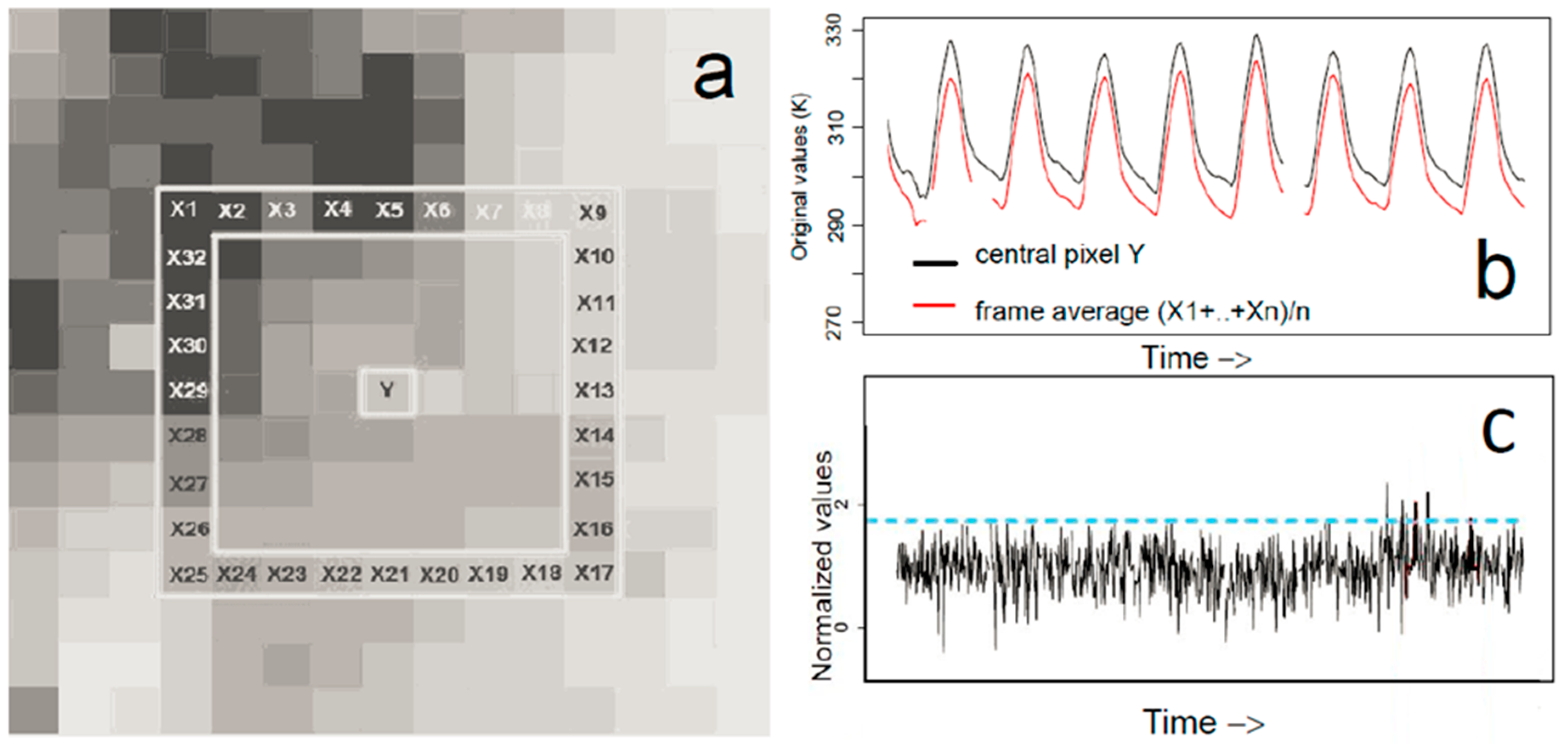
The normalization step suppresses patterns common between the central pixel and an open frame of neighboring pixels. Such patterns could be the diurnal cycle, seasonal effects, humid conditions extending in large areas, or a heat wave. Every pixel value is divided by the average value of a square frame of neighbor pixels (Figure 1). This process is repeated for every pixel of every image in the dataset. After normalization, only localized fluctuations remain and are highlighted in the resulting normalized time series.
An identical frame size is used in all study areas to obtain comparable results. The assumption is that anomalous thermal emissions caused by stress accumulation would be more pronounced over a stressed area. We therefore use larger frames than that area to highlight potential anomalous emissions by applying the normalization. Following Saradjian and Akhoondzadeh [40], the area of stress accumulation is estimated based on the definition of earthquake preparation area given by Dobrovolsky et al. [41]. Dobrovolsky et al. [41] describe a spherical “region of earthquake preparation” defined as a function of the magnitude of an impending earthquake. Rupture length is also taken into account for the decision on frame size, because it could give a first indication of the spatial extent of stress accumulation. Moment magnitude can be used to approximate rupture length based on empirical relationships [42], even though this relationship may vary across different locations.
We set the frame size based on the largest event in our earthquake list: the Kaikoura Mw 7.8 thrust rupture in New Zealand. Its preparation area according to Dobrovolsky et al. [41] has a diameter of 68 km, slightly smaller than 14 pixels in our image datasets. The expected rupture length based on Wells and Coppersmith [42] is 113 km; Shi et al. [43] report it as approximately 116 km on-land, estimated across at least 12 major fault sections. The frame is therefore chosen to have a side length of 29 pixels (145 km), which exceeds the extent of both the estimated earthquake preparation area and the rupture length in all earthquake cases of this study.
2.3.3. Anomaly Detection
The result of the first step is a time series with normalized values. In this time series, normalized values that exceed or are equal to a threshold equal to the mean plus twice the standard deviation of the series (μ + 2σ) are flagged as anomalies. Thus, in our study, an anomaly is consistently defined in all parts of all datasets as a departure higher than +2 standard deviations of the temporal average value of a pixel relative to its neighbors.
The choice of μ + 2σ threshold is in accordance with previous research on detection of earthquake-related anomalies [3,44,45,46]. The threshold is determined by each pixel’s series separately, and is thus dynamically adjusted to local environmental conditions. Furthermore, it is applied uniformly to the whole image, allowing for detection of anomalies without a priori knowledge on where anomalies may appear. Sensitivity analysis of the original method showed that this threshold could capture fluctuations as low as +2K/+3K compared to surroundings of lower/higher background variability [27]. For the possibility that this threshold may also capture lesser environmental influences distorting the statistical evaluation of the results, we repeat the same analysis with a stricter μ + 3σ threshold.
2.3.4. Anomaly Density Calculations
This step includes counting the number of anomalies per unit time, for four spatial zones describing different distances from an earthquake epicenter, and for different time periods (see Table 2 for spatial and temporal details).
A distinction between pre-, post-, and co- seismic periods is suggested by previous research, especially considering the co-seismic period [25]. Pre-seismic periods are considered as a time of stress accumulation. Potential anomalies related to this stress accumulation are expected to appear closer to the time of the rupture [30,47]. A co-seismic period is considered to be the time of rupture and stress release. Thermal anomalies appearing in this time would be related more to friction and the rupture itself rather than stress accumulation. Post-seismic periods follow the rupture and have less stress than the pre-seismic periods, since part of the accumulated stress has been released during the rupture. We define co-seismic periods as 24 h before and 24 h after an earthquake. All events of Mw > 5.5 that happen more than 24 h after another event are seen, in this definition, as separate. Pre- and post-seismic periods of equal duration (two months) are defined for comparability and based on literature on the appearance of earthquake-related anomalies (e.g., [48,49,50]). In periods later and earlier than these, earthquake related anomalies should be unlikely.
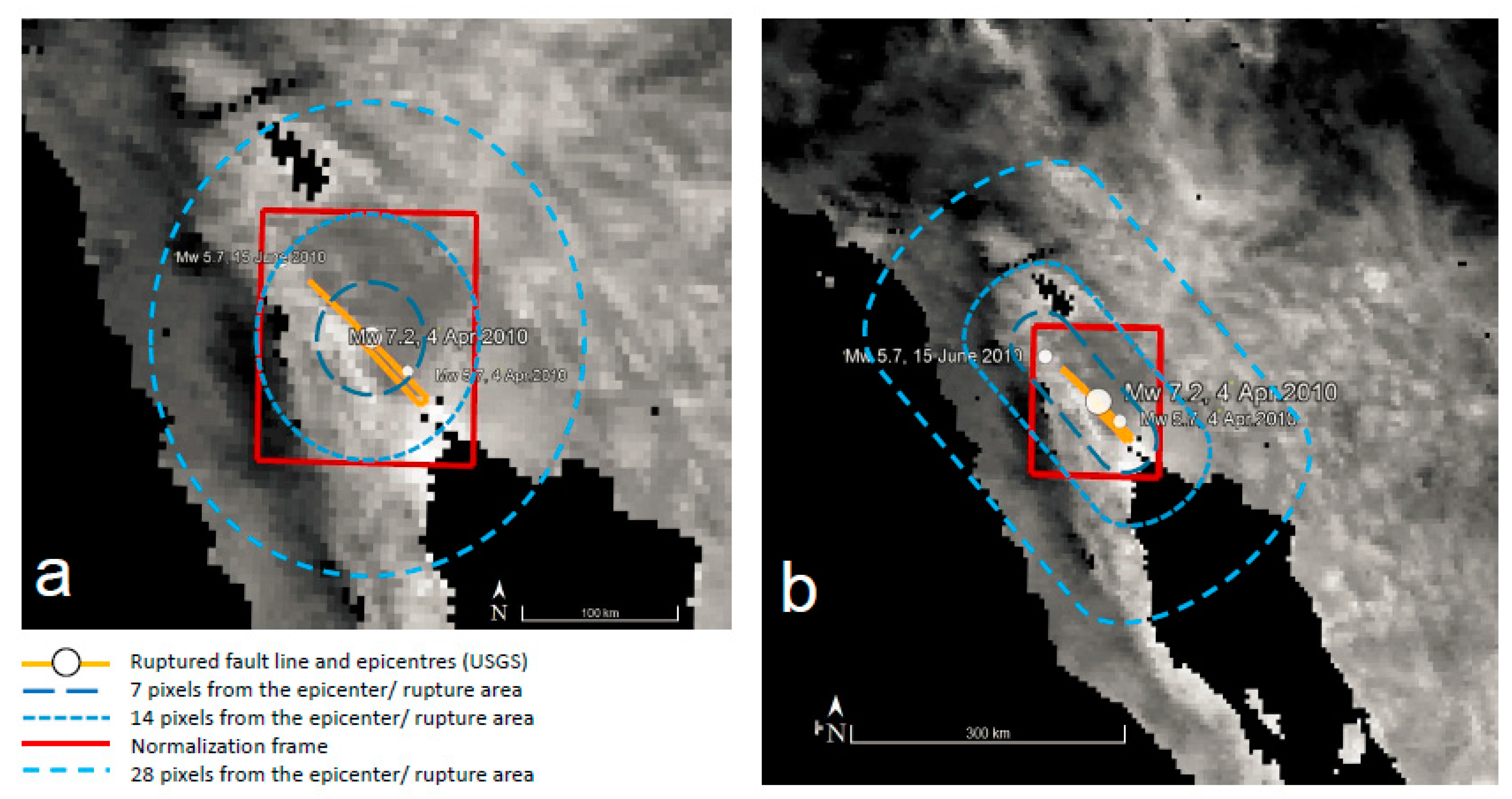
This study includes earthquakes which may be considered as parts of longer earthquake sequences. The sequences are characterized by a higher frequency of low-medium magnitude events than in the rest of the earthquake catalog. It could be argued that, in these cases, stress is being released not in a single rupture but through a sequence of ruptures. To account for such prolonged sequences, the analysis is done twice: once with a 48 h-long co-seismic period and once with a prolonged co-seismic period, adjusted to cover the duration and spatial extent of each sequence. When prolonged co-seismic periods are used, distance zones are defined with regard to the ruptured area, which includes the ruptured fault and epicenters of all large earthquakes in the sequence (Figure 2). Analysis is performed on both standard and adjusted co-seismic periods in the cases described in Table 2.
The total number of anomalies in each zone and period is divided by the total number of available observations in the corresponding zone/period. The result is anomaly density in different periods at different distances from each earthquake. The same processing (normalization-anomaly detection-calculation of anomaly density) is repeated in years with and without earthquake occurrence.
2.3.5. Statistical Analysis
Statistical analysis follows to evaluate detection results based on the hypothesis that a higher anomaly density should be found in areas spatially closer to the earthquake, and in periods shortly before or during the earthquake and only in the years with an earthquake.
A three-way mixed analysis of variance (ANOVA) analysis allows to test for significant combined effects among three factors of interest: time period, distance zone and earthquake/no earthquake year.
There are several possible outcomes of such an analysis. One is that there is a statistically significant combined effect of time period and distance zone only in the earthquake year. This is expressed as a significant three-way interaction effect between time period, distance zone and earthquake year. Such a finding can confirm the hypothesis only if the interaction between them shows that there is a higher anomaly density before or during the earthquake. If the three-way interaction shows a higher anomaly density after the earthquake, then the hypothesis is rejected and anomaly density cannot be considered as a precursory or co-seismic phenomenon. If no significant three-way interaction is found, the hypothesis is rejected.
Another possible outcome is that there is a statistically significant combined effect of any two factors, regardless of the third factor. For example, the combination of time period and distance zone may have a statistically significant effect also in the non-earthquake year. Such an effect may be present for reasons other than an earthquake occurrence, and as a result this finding does not confirm the hypothesis. This condition is expressed as a two-way interaction effect, only between two factors. A third possible outcome is that any of the factors (time period, distance zone, earthquake year) separately affect anomaly density, regardless of the effect of their combination. For example, anomaly density may differ between time periods in the whole study area, regardless if there is an earthquake or not. This is expressed as a statistically significant simple main effect, separately for each factor. Such effects indicate that the period, the year and/or the location affect anomaly density regardless of earthquake occurrence, and as a result this finding does not confirm the hypothesis. The last possible finding is that there is no statistically significant interaction between the factors (they have no combined effect on anomaly density) or that there is no significant simple effect of each factors separately. The absence of simple and/or two-way interaction effects does not provide information for the hypothesis. The only finding that can confirm or reject the hypothesis is the presence or absence of a significant three-way interaction.
3. Results
3.1. Anomaly Detection
This section presents results of the anomaly detection. Examples, highlighting the results of the spatial and temporal processing, are shown for the earthquakes of Emilia Romagna, Italy, in 2012 (Figure 3) and Baja California, Mexico in 2010 (Figure 4). These results are compared to results of the same periods and regions in 2011 and 2016, respectively, when no earthquakes of Mw >5 are recorded in these areas.
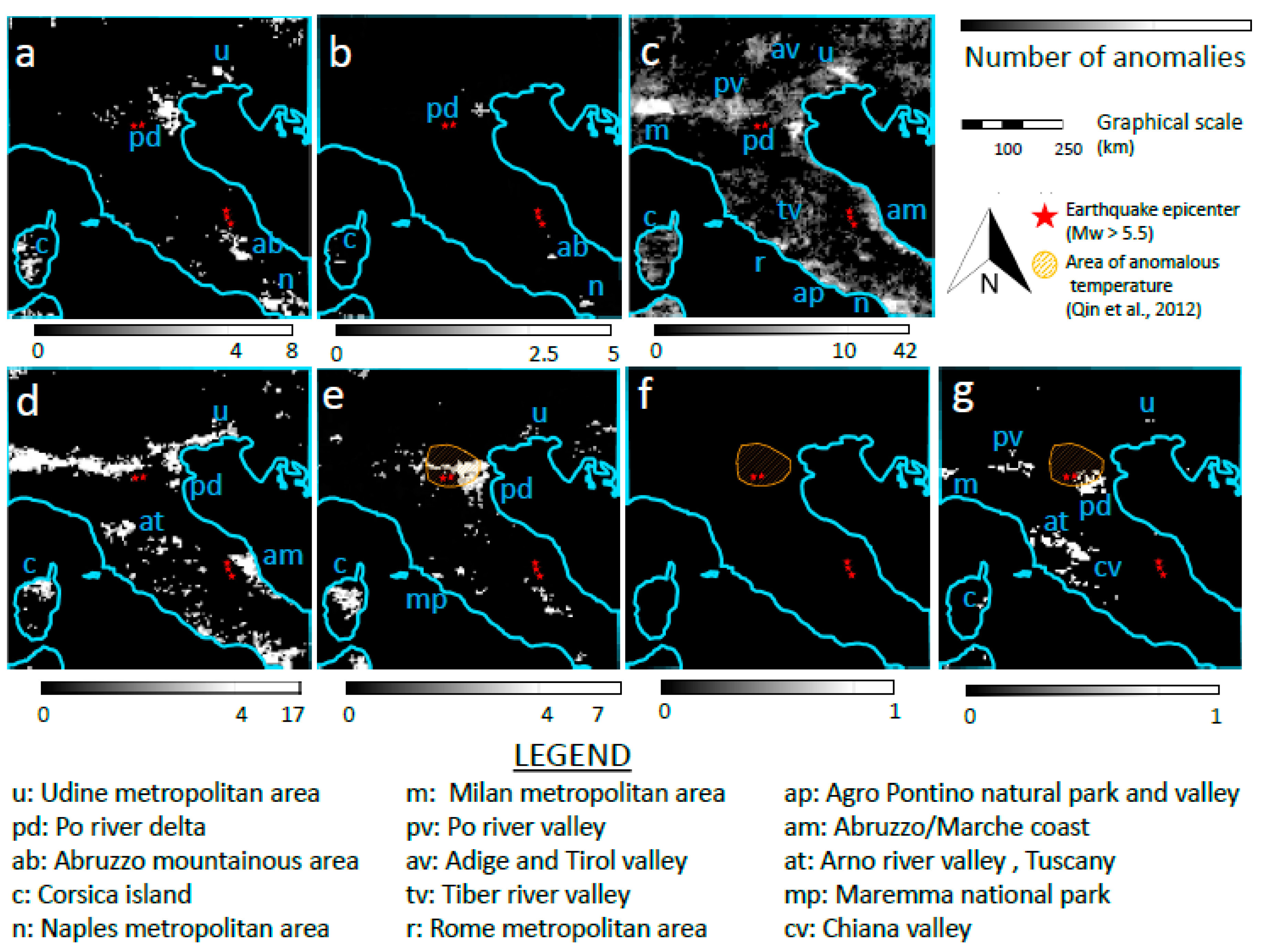
The spatial distribution and the number of anomalies detected in the co-seismic period of the first earthquake of 2012 (19–21 May, 48 time observations in total, see details in Table 1) is shown in Figure 3a. The earthquake epicenters of Emilia Romagna are shown with red stars in the north. The cluster of anomalies closest to the earthquake epicenter appears around 50 km to the east. This cluster (designated pd in Figure 3) is approximately 100 km long and 50 km wide. The highest number of anomalies in this cluster, for the whole co-seismic period, is six of a total of 48 observations. The anomalies of this cluster appear in the morning and early afternoon, mostly between 7:00 a.m. and 2:00 p.m., and then disappear. Scattered anomalous pixels can be seen at the same distance from the earthquake, but towards the west. At a distance of around 180 km to the northeast of the earthquake epicenter, another, less spatially extended, cluster of anomalies (u) can be seen. The core of this cluster covers 25 × 25 km and has the highest number of anomalies in time for the whole study area (8 anomalies in 48 observations). More clusters of anomalies appear towards the south of the earthquake. One cluster (ab) appears at approximately 330 km SE of the epicenter, close to the area where the earthquakes of Norcia, Visso and Amatrice occur over four years later (shown in Figure 3 with three red stars in the south). The highest number of anomalies in cluster (ab) is also 6 out of 48 observations, like in the cluster closest to the earthquake. At 500 km SE of the earthquake, a more extended complex of clusters (n) is visible with a high number of anomalies (8 anomalies in the 48 observations, the highest of the whole study area). Finally, a cluster of anomalies (c) appears on the southwestern end of the island of Corsica, approximately 600 km SW of the earthquake epicenter. It has fewer anomalies (4 in 48 observations) and extends to an area as big as the cluster closest to the earthquake.
When the detection threshold is increased to μ + 3σ (Figure 3b), only the highest normalized values are considered anomalous and less anomalies overall are detected. Smaller clusters of anomalies are visible in the study area. The cluster (pd) closest to the earthquake epicenter is still visible and has 4 anomalous values in 48 observations, similar to the clusters of Corsica (c) and central Italy (ab) which are located further than 300 km from the earthquake epicenter. The highest number of anomalies recorded in time is 5 anomalies in 48 observations and can be found in cluster (n), 500 km SE from the earthquake. Cluster (u) is not visible.
When a longer co-seismic period is considered (19–31 May, using the μ + 2σ threshold), to cover all earthquakes of the 2012 sequence, more anomalies are detected (Figure 3c). The previously identified clusters—(pd), (c), (n), and (u)—remain but are now more spatially extended. The most extended, and new, cluster is located 200 km northwest of the earthquake epicenter. This cluster (m) shows the highest number of anomalies in the image, 42 in the 240 observations compared to the up to 26 anomalies out of 240 observations close to the epicenter. An area of anomalies (shown as pv, with 200 km maximum length and 500 km maximum width) connects clusters (m) and (pd). More clusters of anomalies appear along the east (ap, r, tv) and the west (am) coast of Italy, and on the islands of Corsica (c) and Sardinia (just south of cluster c).
When the same processing is applied for the co-seismic period of 19–21 May in a year without large earthquakes (2011, Figure 3d), similar patterns are observed as compared to the year with earthquake (2012, Figure 3a,c). Previously identified clusters in the north and south (m, pd, u, n) are again visible. The anomalies in the north are connected in an extended cluster with maximum length of ~100 km and a width of ~500 km (pv). Clusters appear in the center of Italy (at) and at the east coast (at, am). Scattered smaller clusters are visible throughout central Italy. The maximum number of anomalies in the year without earthquake is higher than in the year of the earthquake (17 out of 48 observations in 2011, compared to 8 out of 48 observations in 2012) and is found in cluster (m).
Anomalies have been reported to appear earlier than one day before the earthquake. For the earthquakes of the example from Italy, Qin et al. [57] report “local temperature enhancements around the epicenters on the night of May 12 2012, i.e., 8 days before the 20 May, 2012 earthquake”. They present an anomaly on an image corresponding to 8:00 p.m. on 12 May, 2012 (shown in Figure 3e–g as the shaded area). They find anomalies at the same location in an image showing daily average temperatures of 12 May 2012. We detect no anomalies in the image of 8:00 p.m. (Figure 3f). In terms of daily averages, Figure 3e shows the total numbers of anomalies we detected for the full day of 12 May 2012. A cluster of anomalies (pd) is visible close to the earthquake epicenter, which is the most spatially extended cluster in the image. Half of the area of the cluster coincides spatially with the anomaly reported by Qin et al. [57]. The highest number of anomalies in this cluster (but not in the whole image) is six out of a total of 24 observations, and all six appear between the morning and the early afternoon. A cluster of anomalies of the same intensity but covering a slightly smaller spatial extent than the one close to the earthquake, is visible in Figure 3e, over the island of Corsica (c). Clusters (n) and (ab) are also visible but have smaller spatial extent than in the co-seismic period. The highest number of anomalies in the image, that is 7 out of a total of 24 observations, appears in cluster (mp) on the west coast of Italy.
Cluster (pd), which is visible to the east of the earthquake epicenters in the pre- and co-seismic period of 2012, is also visible in other years and days. An example from a post-seismic period (27 September 2011) is shown in Figure 3g. On that day the cluster covers the earthquake epicenter and partially coincides with the area where Qin et al. [57] found an anomaly in 2012. Clusters (m), (at), (pv), (u), (at), and (c) are also visible.
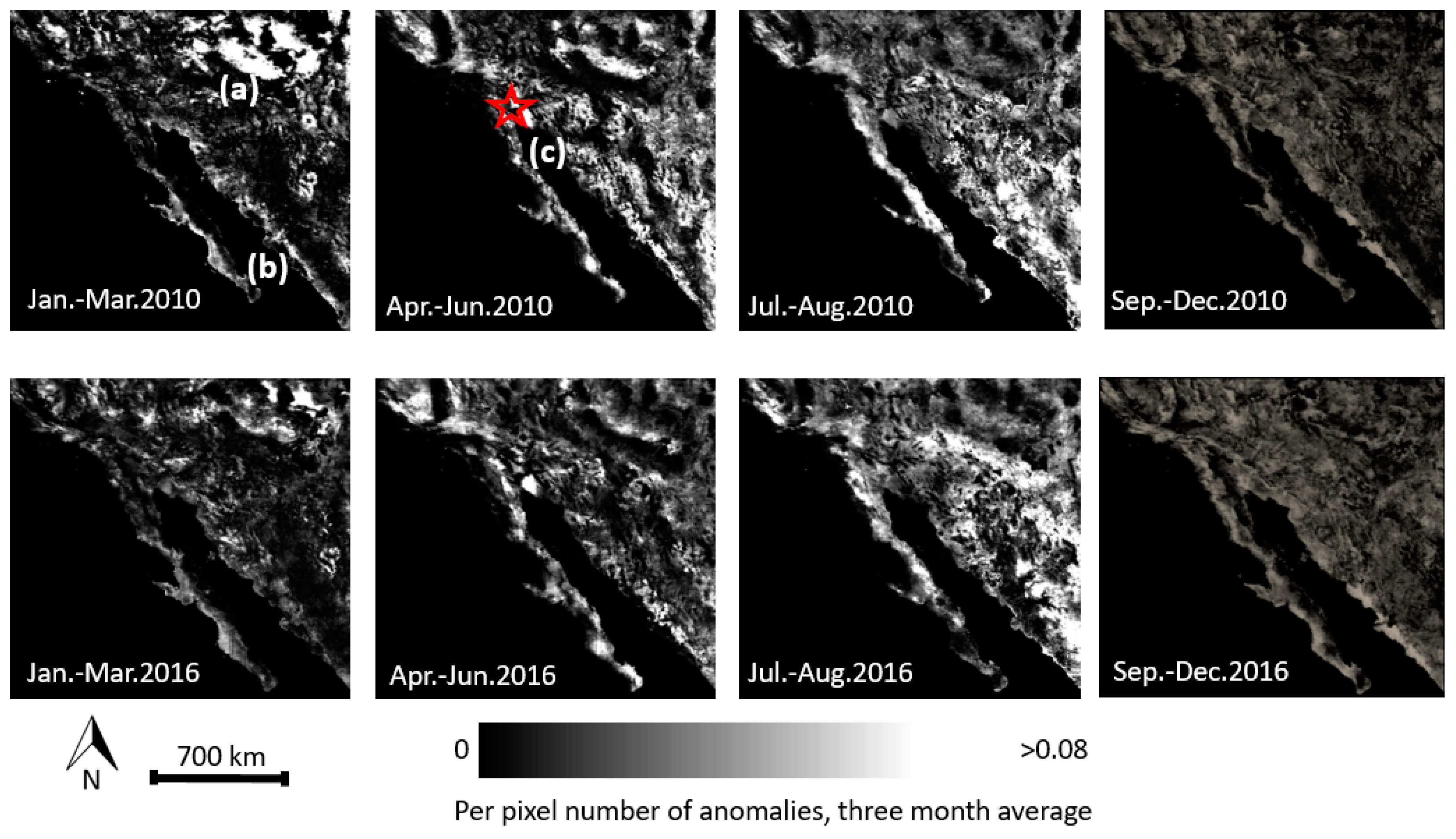
For a more synoptic presentation of the spatiotemporal distribution of detected anomalies, we summarize and plot numbers of anomalies for longer periods. An example is shown in Figure 4 for the study area of Baja California. In the figure, anomalies are presented as three-month averages for two years: 2010 (year of the earthquake) and 2016 (year without earthquake). The area (c) closest to the earthquake shows higher numbers of anomalies between April and June. This is a recurrent phenomenon rather than an earthquake-related effect, because it appears in the earthquake year 2010 (earthquake epicenter shown with a red star) but also in 2016. The mountainous areas (a) in Arizona (Grand Canyon, Mongolon Rim) show a higher number of anomalies from the beginning of the year until June, in both years (less pronounced in 2016). The mountain range of the Sierra Madre Occidental (b) produces anomalies throughout the year, most prominently between September and December.
In the examples above, but also in all studied areas and periods, localized anomalies are found throughout the duration of the datasets. Clusters of anomalies with high intensity appear at different distances from the earthquake epicentre. In Italy, the highest number of anomalies is not found in the cluster closest to the earthquake. The cluster closest to the earthquakes of Emilia Romagna is also present in the year without an earthquake, and at different times of the year (May, September). In Mexico, the area close to the earthquake shows anomalies between April and June in both years (with and without earthquake).
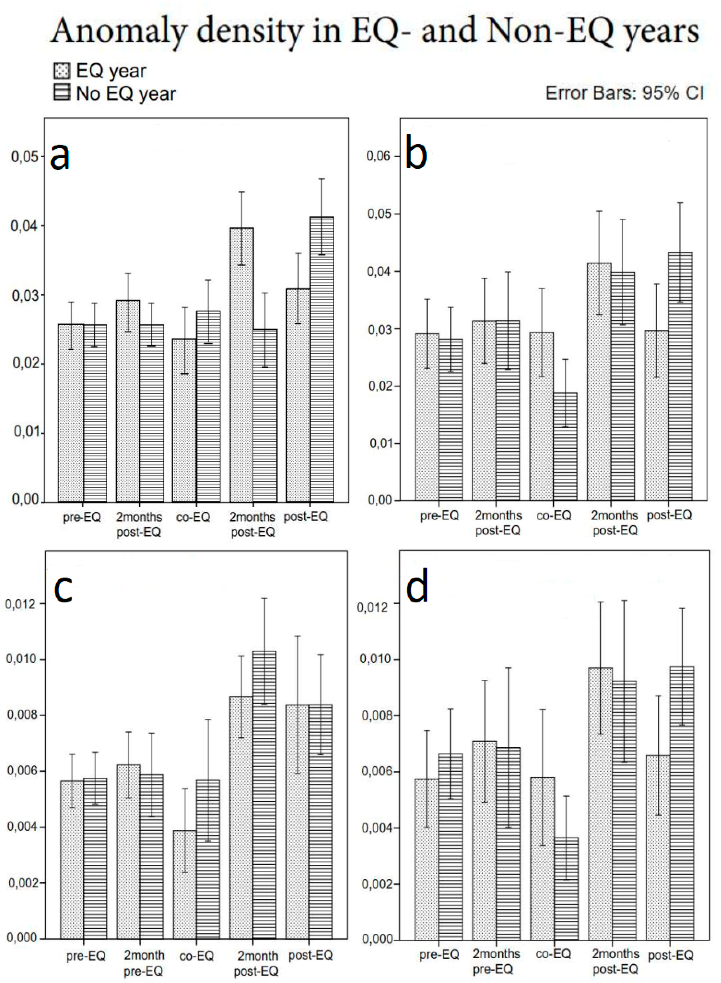
We calculate anomaly density values for each spatial zone and period, to have comparable results in periods of different duration (for example, the co-seismic period of 48 h and the pre-seismic period of 2 months). Anomaly density values for all earthquakes are provided as Supplementary (Dataset S1—S4) of this manuscript. The mean anomaly density of spatial zones further from the earthquake (distance > 70 km) is higher than in zones closer to the earthquake. In terms of time, post-earthquake periods have the highest mean anomaly density and the co-seismic period has the lowest (Figure 5).
3.2. Statistical Analysis
The results of anomaly detection, described above, show presence of anomalies in years with and without earthquakes. Statistical analysis is performed to conclude if there is a significant relation between the occurrence of earthquakes and detected anomalies. Such a relation would be established only if anomaly density is higher close to earthquake epicentres, before/during the earthquake and only in the years with an earthquake. The analysis is repeated for the following experimental configurations: use of different thresholds (mean + 2σ, mean + 3σ) and with/without adjustment of the co-seismic period. Additionally, the analysis shows the statistical significance of the differences of average anomaly density between different zones/periods (Figure 5). Table 3 presents the results of each ANOVA test, in the different experimental configurations. A technical description of the tests is provided in Appendix A.
In all experimental configurations, there is no statistically significant three-way interaction between earthquake year, period, and distance zone (Line 1, Table 3). This means that there is no significant difference in anomaly density found only in the year of the earthquake. It is thus not possible to say that there are more anomalies close to the earthquake, before/during the earthquake, and only in the year of the earthquake. Any differences between the anomaly density in different zones and periods are present in earthquake and no-earthquake years alike, and they cannot be attributed to the occurrence of the earthquake. This is the only statistical result related to the hypothesis that there is a relation between earthquakes and anomalies, and the findings reject the hypothesis.
Statistical analysis further provides indications of how anomaly density differs in different years, locations and periods, regardless of the earthquake (Lines 2–7 of Table 3). Regardless of the experimental configuration, location relative to the earthquake epicenter does not affect anomaly density at any time (lines 2, 4). Distance from the earthquake by itself has no significant effect on anomaly density (line 6). Anomaly density differs with period and year, depending on the experimental configuration (line 3). Period by itself has a statistically significant effect in anomaly density of different years and distance zones (line 5). This effect is found in all cases except when an adjusted co-seismic period is applied with a μ + 3σ threshold. Year by itself has a significant effect on anomaly density only when adjusted co-seismic periods are applied in combination with a μ + 3σ threshold (line 7).
Overall, the result of the statistical analysis is that regardless of the applied threshold and the definition of the co-seismic period, there is no significant effect of the earthquakes in the anomaly density measured across distance zones and periods.
4. Discussion
4.1. Choice of Data Input
Our study uses LST data derived from geostationary sensors to investigate the presence of local increases in LST which may be linked to earthquake occurrence. The choice of data is critical for the study. As suggested by previous research, geostationary-based LST data series are less affected by uncertainties related to image co-location and observational conditions [38]. Cloud masking and atmospheric corrections applied for LST derivation minimize the risk that detected anomalies are related to atmospheric effects and clouds, rather than surface processes [31]. To further decrease the propagation of input uncertainty throughout detection, we analyze only pixels with estimated LST retrieval errors less than 2K. Uncertainties related to sensor noise, surface emissivity/land cover type, and water vapor [35] above this limit are therefore accounted for in our detection results. The spatial and temporal resolution of the data allow for examination of the spatiotemporal coincidence between detected anomalies and earthquakes, and for detailed study of the extent and duration of LST increases. These are further discussed in the following sections.
4.2. Spatial Extent of Anomalies
In published research, the spatial extent of detected anomalies is often not clear. For example, Akhoondzadeh et al. [7,19] and Pulinets et al. [59] study the 6.4 Mw earthquake of Ahar, NW Iran (2012) using data from meteorological stations. Such data have very limited spatial cover and cannot describe the full extent of detected anomalies. Even when Akhonzadeh et al. [7] use satellite data (MODIS LST), they confine their anomaly detection to an area 5 × 5 km over the earthquake epicenter. Other researchers study larger areas using data with coarse spatial resolution. For example, Alvan et al. [8], who study the event of Baja California (2010), report anomalies in gridcells of a spatial extent of 2° × 2°. For the same event Jie and Guangmeng [22] find anomalies in an area of 1° × 1° over the epicenter. Qin et al. [9,57] and Wu et al. [60], who report anomalies in New Zealand (2010) and Italy (2012), use data with a 2° × 2° spatial resolution. When reported anomalies extend to degrees latitude/longitude, it is not possible to trace back in detail their exact origin and their spatial relation to faults and other potential causative processes. In our study, anomaly detection is based on gridded satellite data of 5 × 5 km spatial resolution, which allows a more detailed description of the location of anomalies with respect to the earthquake. For example, reported anomalies in Italy and Mexico, with an extent of 2° × 2° [22,57] spatially coincide in our results with anomalies scattered over different locations.
Furthermore, the normalization procedure we apply ensures that detected anomalies have a spatial extent less than the normalization frame (up to 18,225 km2). It therefore makes it possible to distinguish localized anomalies from larger-scale weather patterns, image-wide diurnal patterns, and climatic trends. That could explain the cases when other researchers find anomalies and our results show none. In our findings, extended patterns, like the thermal inversion described by Qu et al. [29] as a more probable reason for the appearance of a pre-earthquake anomaly in Mongolia, are suppressed. An unusually warm day in the whole study area is not linked to the earthquake, and anomalies are not masked by unusually cold days.
4.3. Distance between Anomalies and Earthquakes
In the first reports that describe earthquake-related thermal anomalies, the distance between anomalies and earthquakes was not taken into account. Anomalies were traced as far as 500 km away from the epicenter [61] or further [28,62]. Piroddi and Ranieri [63] argue that observable phenomena further than 60 km from the earthquake, even if they were spatially associable to the seismic event, they would not be practically useful as precursors because the potential alarm areas would be too big. We address the issue of the distance between anomalies and epicenters by classifying all detected anomalies in four different spatial zones, based on their distance from the earthquake. The two zones closest to the earthquake correspond to the suggestion of Piroddi and Ranieri [63] and are used to distinguish areas in the more or less immediate vicinity of the earthquake. In our study areas, anomaly density is, on average, higher in zones further away from the earthquake, and the analysis shows that even this difference is not statistically significant. Since no difference is found in anomaly density between the zones, the location of the earthquake has no effect on anomaly density.
4.4. Temporal Resolution
Previous studies use daily averages or one image per 24 h for detection (e.g., [7,19,64]). We use one image every hour and construct hyper-temporal time series to allow the study of transient anomalies. The use of LST over the whole diurnal cycle provides information to explore temporal persistence and potential causes of the anomaly. In the example of Italy, the anomaly closest to the earthquake is found only in six images in the co-seismic period of 48 observations. It appears early in the day (between 7:00 a.m. and 2:00 p.m.) and it is recurrent in different days and years. There is no physical evidence to support why earthquake effects appear, disappear and reappear within hours at preferred times of the day, and persist in years without an earthquake. Furthermore, by using the full diurnal cycle we consider the serial dependence of LST observations and utilize it to describe normal behavior. In contrast, choosing only specific samples (only a few night-time images, for example) would not address LST temporal dynamics and could introduce bias in anomaly detection and statistical analysis.
4.5. Temporal Coincidence with Earthquakes
We examine complete years, and the same area is examined with and without earthquake occurrence. This allows us to test for presence of anomalies in periods without earthquakes. Previous studies often test a variety of periods but only shortly before and after the earthquake [8,19,22]. This leaves the possibility that similar anomalies may be a regular occurrence appearing throughout the year(s) without any earthquake effect, as found by Blackett et al. [26]. Our results show that anomalies in the vicinity of earthquake epicenters, as well as everywhere in the study areas, appear throughout the years, regardless of an earthquake occurrence.
4.6. Statistical Analysis
We investigate the link between earthquakes and anomalies with the application of statistical analysis following the suggestions of Eneva et al. [25]. We take all detected anomalies into account and extend our analysis in years with and without earthquakes. The statistical analysis shows that detected anomalies appear regardless of earthquake occurrence, in terms of time and distance from an earthquake epicenter. These results are in agreement with Eneva et al. [25], who applied a similar statistical design reaching the same conclusions. Zhang et al. [65], following a different statistical scheme, also conclude that in their data the correlation between occurrence of earthquakes and detected anomalies was very low. Changing the anomaly threshold or the period of investigation (to a larger co-seismic period) in our work, does not change the results. Furthermore, no recognizable patterns are found in the case of earthquakes that repeatedly appear in similar locations (Italy, New Zealand and Oklahoma).
4.7. Potential Sources of Anomaly
Potential earthquake-related effects on LST may exist but remain undetected if they are weaker than, or at least similar to other sources of LST variability. In terms of the potential sources underlying the anomalies we detect, locations over urban centers, rough terrain and complex topography, agricultural activity, and wetlands appear to have high numbers of detected anomalies throughout the study areas and periods (see for example Figure 3 and Figure 4).
Rough terrain and complex topography can lead to differential heating of surfaces more or less exposed to solar irradiation, resulting in differences in the thermal emissions (and as a result, the LST) recorded from different locations. Topography and elevation contribute to atmospheric phenomena, like temperature inversions, which may lead to increased recorded emissions [66]. The surfaces and the human activities that occur in urban areas increase LST and LST variability [67,68]. Vegetation cover, and subsequently LST, varies throughout the year in agricultural areas, as does the presence of water. Water in the soil and in wetlands affects registered LST through its emissivity, thermal behavior and phase transitions. Liquid water and moist soil have higher heat capacity and emissivity than dry soils [69]. Total atmospheric water vapor increases absorption and attenuates the registered thermal emissions [70], while phase transitions like vapor condensation release latent heat in the atmosphere. It should be noted that such effects would have more impact on detection methodologies which rely only on spatial image statistics for anomaly detection. In our results, however, we detect anomalies based on the temporal dynamics of normalized series, and the above-mentioned localized effects and/or their combinations are a source of anomaly when they fluctuate temporally. This is reflected in the statistical analysis, which indicates weak effects of time (period/year relative to the earthquake) and not of space, in the density of detected anomalies (Table 3).
These observations vary among the studied areas and cannot be further explored in the frame of this study. Detailed examination in combination with additional data (emissivity, land use/land cover) could provide more information on the sources of natural LST variability and their interactions.
4.8. Limitations
In order to set the detection threshold and to define co-seismic periods, we use information from literature on earthquake preparation area definition, fault lengths and earthquake sequences. However, we acknowledge that existing literature is descriptive rather than exploratory. To this moment, there is no physically-based detection threshold or definition of a co-seismic period. In recognition of this, we test different settings to evaluate the sensitivity of our results to those settings. We find that the main results are robust to the use of different settings, and they remain the same regardless of the use of stricter detection thresholds or adjusted co-seismic period.
Regarding the size of normalization frame, we set it based on literature on the earthquake preparation area. It may be argued, however, that there may be links between earthquakes and anomalies appearing hundreds of kilometers away from the earthquake without being present in the immediate proximity of the event, or that earthquake-related influences extend over areas larger than 18,225 km2. In such cases, the frame we apply may be considered too strict and a future researcher could choose to apply normalization frames of different sizes. To this moment, the theoretical background behind such occurrences is not yet established and their precursory value may currently be limited, as discussed earlier.
We have examined 20 earthquakes. This collection is diverse in terms of fault mechanism, climatic conditions, topography, and land cover, but it still is only a sample. An ideal sample would contain multiple similar large earthquakes with different focal mechanisms, in areas with different local conditions. Their occurrence should be covered by comparable satellite sensors and unperturbed years should be included for statistical analysis of anomaly occurrence. Further research, supported by the release of longer LST datasets, should be systematically extended to include more earthquake cases, of different characteristics and from different regions. This could increase representativeness of the sample and reduce the variability in the results of statistical analysis.
5. Conclusions
The study of hyper-temporal geostationary-based LST records to detect anomalous increases of spatial extent up to 18,225 km2 in ten land-based, earthquake-prone areas worldwide, yields anomalies throughout the year-long datasets and throughout the study areas, regardless of the occurrence of an earthquake. The results show no statistically significant difference in anomaly density between years with and without earthquake, in the same location; and no difference among locations closer to or further from the earthquake, within the same study area and year. No recognizable patterns are identified when earthquakes occur in the same region in different years. We conclude that the 20 earthquake events we tested do not significantly affect thermal anomalies as observed in geostationary satellite LST data on the investigated scales. The findings suggest that if an earthquake-related effect exists, it is weaker than other environmental influences or spatially more extensive than what is tested.
Supplementary Materials
The following are available online at https://0-www-mdpi-com.brum.beds.ac.uk/2072-4292/11/1/61/s1, Dataset S1: Anomaly densities, mean + 2σ threshold, 48-h co-seismic period; Dataset S2: Anomaly densities, mean + 2σ threshold, adjusted co-seismic period; Dataset S3: Anomaly densities, mean + 3σ threshold, 48-h co-seismic period; Dataset S4: Anomaly densities, mean + 3σ threshold, adjusted co-seismic period.
Author Contributions
Conceptualization, M.v.d.M., E.P., C.H., and H.v.d.W.; Methodology, M.M, E.P., H.v.d.W., and C.H.; Software, E.P., H.v.d.W.; Formal analysis, E.P.; Resources, E.P.; Data curation, E.P.; Writing—original draft preparation, E.P.; Writing—review and editing, M.M, C.H., and H.v.d.W.; Visualization, E.P.; Supervision, M.v.d.M., C.H., and H.v.d.W.
Funding
Funding for all authors related to this work was provided by the University of Twente, The Netherlands.
Acknowledgments
LST datasets were obtained online from the Copernicus network (Copernicus Global Land Services, https://land.copernicus.eu/global/products/lst. Earthquake data were retrieved from the online USGS earthquake catalog (https://earthquake.usgs.gov/earthquakes/search/). Statistical analysis was performed using the software IBM SPSS statistics for Windows, Version 24.0.
Conflicts of Interest
The authors do not perceive any financial or affiliation-related conflict of interest with respect to this study.
Appendix A
Appendix A1. Statistical Analysis of Anomaly Density Data, μ + 2σ Threshold, No Adjustment of the Co-Seismic Period
In the data there were 14 outliers, as assessed by examination of studentized residuals for values greater than ±3. The outliers are traced back in the anomaly density of Myanmar (2012), Baja California (June 2010), and New Zealand (2010) and were spread across distance zones and periods. They were kept in the data because they did not materially affect the results as assessed by a comparison of the results with and without the outliers. Anomaly density was not normally distributed in all cases, as assessed by a Shapiro-Wilk test. Transformation of the data did not establish normality in all cases so analysis was performed on the original values. There was homogeneity of variances, as assessed by Levene’s test for equality of variances (p > 0.05). Mauchly’s test of sphericity indicated that the assumption of sphericity was violated for the two-way interaction, χ2(9) = 113.503, p < 0.001. Thus, the Greenhouse-Geisser correction was applied (following Maxwell et al. [58], ε < 0.75).
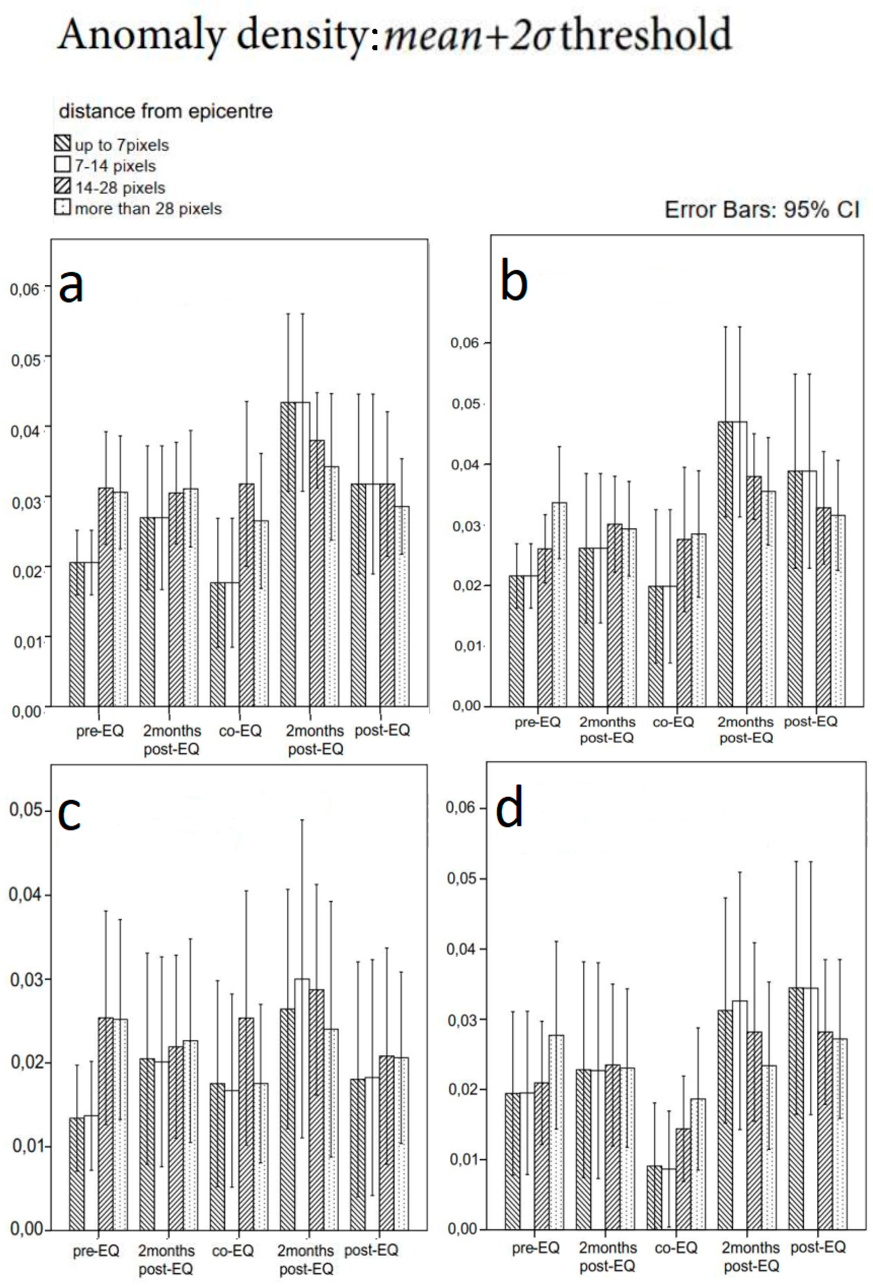
No significant interaction was found between earthquake occurrence, period and distance from the earthquake, F(6.094, 134.060) = 0.162, p = 0.987, partial η2 = 0.007. There was no statistically significant two-way interaction, F(8.914, 196.116) = 1.645, p = 0.106, partial η2 = 0.070 (between period and distance zone); F(3, 66) = 0.844, p = 0.475, partial η2 = 0.037 (between earthquake year and distance zone); F(2.031, 66) = 0.959, p = 0.387, partial η2 = 0.014 (between earthquake year and period). There was a significant simple main effect of period, F(2.971, 196.116) = 11.738, p < 0.001, partial η2 = 0.151 which was present regardless of location or earthquake occurrence. In particular, the two-month post-earthquake period had the highest average anomaly density (0.040 ± 0.026). The lowest mean anomaly density (0.023 ± 0.021) was found in the co-seismic period.
Average anomaly density from all earthquake cases is shown in Figure A1a,b, grouped per period, zone, and earthquake year.
Appendix A2. Statistical Analysis of Anomaly Density Data, μ + 2σ Threshold, with Adjustment of the Co-Seismic Period
In the data there were 18 outliers, as assessed by examination of studentized residuals for values greater than ±3. The outliers are traced back in anomaly density of Myanmar (2012 and 2011), China (2010), Italy (2012) and New Zealand (2010) and were spread across distance zones and periods. They were kept in the data because they did not materially affect the results as assessed by a comparison of the results with and without the outliers. Anomaly density was not normally distributed in all cases, as assessed by a Shapiro–Wilk’s test. Transformation of the data did not establish normality in all cases so analysis was performed on the original values. There was homogeneity of variances, as assessed by Levene’s test for equality of variances (p > 0.05). Mauchly’s test of sphericity indicated that the assumption of sphericity was violated for the two-way interaction, χ2(9) = 82.177, p < 0.001. Thus, the Greenhouse-Geisser correction was applied (following Maxwell et al. [58] with ε < 0.75).
No significant interaction was found between earthquake occurrence, period and distance from the earthquake, F(6.767, 121.798) = 0.596, p = 0.753, partial η2 = 0.032. There was no statistically significant two-way interaction between period and distance zone, F(6.832, 122.971) = 0.574, p = 0.772, partial η2 = 0.031; none between earthquake year and distance zone, F(3, 54) = 2.279, p = 0.090, partial η2 = 0.112; and there was significant two-way interaction between earthquake year and period, F(2.256, 54) = 6.954, p = 0.001, partial η2 = 0.114 regardless of distance to the earthquake. There was also a significant simple main effect of period, F(2.971, 196.116) = 11.738, p < 0.001, partial η2 = 0.151. In particular, the post-earthquake period in no-earthquake years had the highest average anomaly density (0.043 ± 0.026). The lowest mean anomaly density (0.019 ± 0.018) was found in the co-seismic period of no-earthquake years.
Average anomaly density from all earthquake cases is shown in Figure A1c,d, grouped per period, zone and earthquake year.
Figure A1.
Anomaly density using a μ + 2σ threshold and 48 h- or adjusted co-seismic period. Results from all earthquake cases grouped per time period, spatial zone and earthquake year. (a) Earthquake years, 48-h co-seismic period (b) No-Earthquake years, 48-h co-seismic period (c) Earthquake years, adjusted co-seismic period (d) No-Earthquake years, adjusted co-seismic period.

Appendix A3. Statistical Analysis of Anomaly Density Data, μ + 3σ Threshold, No Adjustment of the Co-Seismic Period
In the data there were 14 outliers, as assessed by examination of studentized residuals for values greater than ±3. The outliers are traced back in anomaly density of Myanmar (2012 and 2011), Baja California (June 2010), Van (2012) and Ahar (2011) and were spread across distance zones and periods. They were kept in the data because they did not materially affect the results as assessed by a comparison of the results with and without the outliers. Anomaly density was not normally distributed in all cases, as assessed by a Shapiro–Wilk’s test. Transformation of the data did not establish normality in all cases so analysis was performed on the original values. There was homogeneity of variances, as assessed by Levene’s test for equality of variances (p > 0.05) except for the case of the pre-earthquake period of non-earthquake years (p = 0.028). Mauchly’s test of sphericity indicated that the assumption of sphericity was violated for the two-way interaction, χ2(9) = 188.861, p < 0.001. Thus, the Greenhouse-Geisser correction was applied (following Maxwell et al. [58], with ε < 0.75).
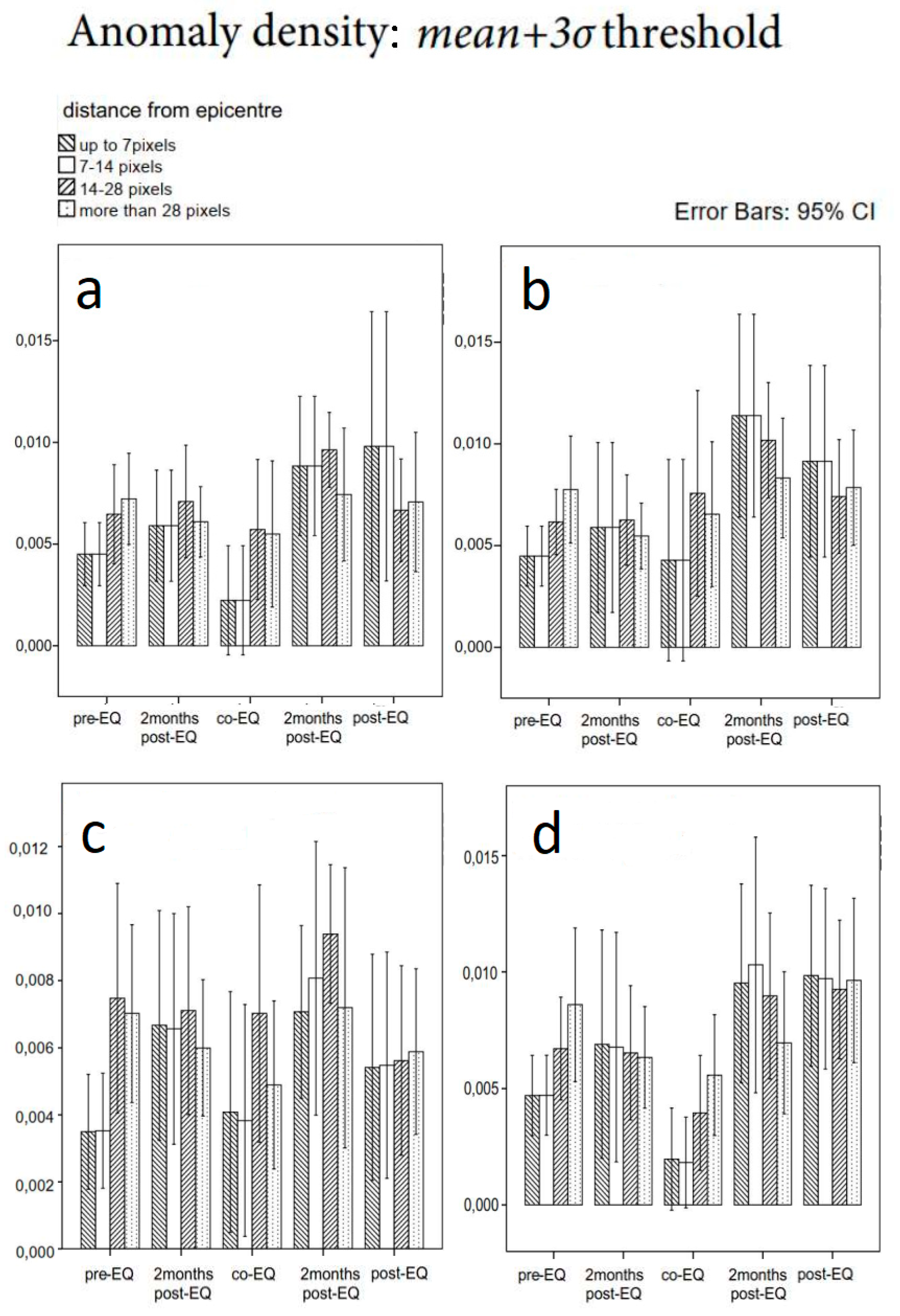
No significant interaction was found between earthquake occurrence, period and distance from the earthquake, F(5.210, 116.355) = 0.148, p = 0.983, partial η2 = 0.007. There was no statistically significant two-way interaction, F(8.905, 198.888) = 1.224, p = 0.282, partial η2 = 0.052 (between period and distance zone); F(3, 67) = 0.008, p = 0.999, partial η2 < 0.001 (between earthquake year and distance zone); F(1.737, 67) = 0.934, p = 0.384, partial η2 = 0.014 (between earthquake year and period). There was a significant simple main effect of period, F(2.968, 116.355) = 9.927, p < 0.001, partial η2 = 0.129 which was present regardless of location or earthquake occurrence. In particular, the 2-month post-earthquake period had the highest average anomaly density (0.0095 ± 0.0073). The lowest mean anomaly density (0.0048 ± 0.0080) was found in the co-seismic period.
Average anomaly density from all earthquake cases is shown in Figure A2a,b, grouped per period, zone and earthquake year.
Appendix A4. Statistical Analysis of Anomaly Density Data, μ + 3σ Threshold, with Adjustment of the Co-Seismic Period
In the data there were 13 outliers, as assessed by examination of studentized residuals for values greater than ±3. The outliers are traced back in anomaly density of Myanmar (2012 and 2011) and Baja California (June 2010) and were spread across distance zones and periods. They were kept in the data because they did not materially affect the results as assessed by a comparison of the results with and without the outliers. Anomaly density was not normally distributed in all cases, as assessed by a Shapiro–Wilk’s test. Transformation of the data did not establish normality in all cases so analysis was performed on the original values. There was homogeneity of variances, as assessed by Levene’s test for equality of variances (p > 0.05) except for the case of the pre-earthquake period of non-earthquake years (p = 0.013). Mauchly’s test of sphericity indicated that the assumption of sphericity was violated for the two-way interaction, χ2(9) = 49.772, p < 0.001. Thus, the Greenhouse-Geisser correction was applied (following Maxwell et al. [58], with ε < 0.75).
No significant interaction was found between earthquake occurrence, period and distance from the earthquake, F(8.507, 155.958) = 0.422, p = 0.915, partial η2 = 0.022. There was no statistically significant two-way interaction between period and distance zone, F(7.604, 139.413) = 0.788, p = 0.608, partial η2 = 0.041 ; neither between earthquake year and distance zone F(3, 55) = 0.626, p = 0.601, partial η2 = 0.033. There was a significant two-way interaction between earthquake year and period, F(2.836, 55) = 6.485, p < 0.001, partial η2 = 0.105. There was a significant simple main effect of period, F(2.535, 139.413) = 6.631, p < 0.001, partial η2 = 0.108 which was present regardless of location or earthquake occurrence; and a simple main effect of earthquake year, F(1, 55) = 14.914, p < 0.001, partial η2 = 0.213. In particular, the post-earthquake period in no-earthquake years had the highest average anomaly density (0.0097 ± 0.0062). The lowest mean anomaly density (0.0036 ± 0.0045) was found in the co-seismic period of no-earthquake years.
Average anomaly density from all earthquake cases is shown in Figure A2c,d, grouped per period, zone and earthquake year.
Figure A2.
Anomaly density using a μ + 3σ threshold and adjusted co-seismic period. Results from all earthquake cases grouped per time period, spatial zone and earthquake year. (a) Earthquake years, 48-h co-seismic period (b) No-Earthquake years, 48-h co-seismic period (c) Earthquake years, adjusted co-seismic period (d) No-Earthquake years, adjusted co-seismic period.

References
- Tramutoli, V.; Corrado, R.; Filizzola, C.; Genzano, N.; Lisi, M.; Pergola, N. From visual comparison to Robust Satellite Techniques: 30 years of thermal infrared satellite data analyses for the study of earthquake preparation phases. Boll. Geofis. Teor. Appl. 2015, 56, 167–202. [Google Scholar]
- Lisi, M.; Filizzola, C.; Genzano, N.; Grimaldi, C.; Lacava, T.; Marchese, F.; Mazzeo, G.; Pergola, N.; Tramutoli, V. A study on the Abruzzo 6 April 2009 earthquake by applying the RST approach to 15 years of AVHRR TIR observations. Nat. Hazards Earth Syst. Sci. 2010, 10, 395–406. [Google Scholar] [CrossRef] [Green Version]
- Ouzounov, D.; Bryant, N.; Logan, T.; Pulinets, S.; Taylor, P. Satellite thermal IR phenomena associated with some of the major earthquakes in 1999–2003. Phys. Chem. Earth Parts A/B/C 2006, 31, 154–163. [Google Scholar] [CrossRef]
- Tramutoli, V.; Di Bello, G.; Pergola, N.; Piscitelli, S. Robust satellite techniques for remote sensing of seismically active areas. Ann. Geofis. 2001, 44. [Google Scholar] [CrossRef]
- Baral, S.; Sharma, K.; Saraf, A.; Das, J.; Singh, G.; Borgohain, S.; Kar, E. Thermal anomaly from NOAA data for the Nepal earthquake. Curr. Sci. 2016, 110, 150. [Google Scholar]
- Lisi, M.; Filizzola, C.; Genzano, N.; Paciello, R.; Pergola, N.; Tramutoli, V. Reducing atmospheric noise in RST analysis of TIR satellite radiances for earthquakes prone areas satellite monitoring. Phys. Chem. Earth Parts A/B/C 2015, 85–86, 87–97. [Google Scholar] [CrossRef]
- Akhoondzadeh, M. A comparison of classical and intelligent methods to detect potential thermal anomalies before the 11 August 2012 Varzeghan, Iran, earthquake (Mw = 6.4). Nat. Hazards Earth Syst. Sci. 2013, 13, 1077. [Google Scholar] [CrossRef]
- Alvan, H.V.; Mansor, S.; Omar, H.; Azad, F.H. Precursory signals associated with the 2010 M8.8 Bio-Bio earthquake (Chile) and the 2010 M7.2 Baja California earthquake (Mexico). Arab. J. Geosci. 2014, 7, 4889–4897. [Google Scholar] [CrossRef]
- Qin, K.; Wu, L.; Santis, A.D.; Meng, J.; Ma, W.; Cianchini, G. Quasi-synchronous multi-parameter anomalies associated with the 2010–2011 New Zealand earthquake sequence. Nat. Hazards Earth Syst. Sci. 2012, 12, 1059–1072. [Google Scholar] [CrossRef]
- Pulinets, S.; Dunajecka, M. Specific variations of air temperature and relative humidity around the time of Michoacan earthquake M8. 1 Sept. 19, 1985 as a possible indicator of interaction between tectonic plates. Tectonophysics 2007, 431, 221–230. [Google Scholar] [CrossRef]
- Panda, S.; Choudhury, S.; Saraf, A.; Das, J. MODIS land surface temperature data detects thermal anomaly preceding 8 October 2005 Kashmir earthquake. Int. J. Remote Sens. 2007, 28, 4587–4596. [Google Scholar] [CrossRef]
- Lu, X.; Meng, Q.Y.; Gu, X.F.; Zhang, X.D.; Xie, T.; Geng, F. Thermal infrared anomalies associated with multi-year earthquakes in the Tibet region based on China’s FY-2E satellite data. Adv. Space Res. 2016, 58, 989–1001. [Google Scholar] [CrossRef]
- Ouzounov, D.; Liu, D.; Chunli, K.; Cervone, G.; Kafatos, M.; Taylor, P. Outgoing long wave radiation variability from IR satellite data prior to major earthquakes. Tectonophysics 2007, 431, 211–220. [Google Scholar] [CrossRef]
- Cervone, G.; Maekawa, S.; Singh, R.; Hayakawa, M.; Kafatos, M.; Shvets, A. Surface latent heat flux and nighttime LF anomalies prior to the Mw = 8.3 Tokachi-Oki earthquake. Nat. Hazards Earth Syst. Sci. 2006, 6, 109–114. [Google Scholar] [CrossRef]
- Dey, S.; Singh, R. Surface latent heat flux as an earthquake precursor. Nat. Hazards Earth Syst. Sci. 2003, 3, 749–755. [Google Scholar] [CrossRef] [Green Version]
- Rezapour, N.; Fattahi, M.; Bidokhti, A.A. Possible soil thermal response to seismic activities in Alborz region (Iran). Nat. Hazards Earth Syst. Sci. 2010, 10, 459–464. [Google Scholar] [CrossRef] [Green Version]
- Liu, D.-F.; Peng, K.-Y.; Liu, W.-H.; Li, L.-Y.; Hou, J.-S. Thermal omens before earthquakes. Acta Seismol. Sin. 1999, 12, 710–715. [Google Scholar] [CrossRef]
- Jordan, T.H.; Chen, Y.-T.; Gasparini, P.; Madariaga, R.; Main, I.; Marzocchi, W.; Papadopoulos, G.; Sobolev, G.; Yamaoka, K.; Zschau, J. Operational Earthquake Forecasting. State of Knowledge and Guidelines for Utilization. Ann. Geophys. 2011, 2011, 54. [Google Scholar] [CrossRef]
- Akhoondzadeh, M. An Adaptive Network-based Fuzzy Inference System for the detection of thermal and TEC anomalies around the time of the Varzeghan, Iran, (Mw = 6.4) earthquake of 11 August 2012. Adv. Space Res. 2013, 52, 837–852. [Google Scholar] [CrossRef]
- Yao, Q.-L.; Qiang, Z.-J. The elliptic stress thermal field prior to M S 7.3 Yutian, and M S 8.0 Wenchuan earthquakes in China in 2008. Nat. Hazards 2010, 54, 307–322. [Google Scholar] [CrossRef]
- Tronin, A. Thermal IR satellite sensor data application for earthquake research in China. Int. J. Remote Sens. 2000, 21, 3169–3177. [Google Scholar] [CrossRef]
- Jie, Y.; Guangmeng, G. Preliminary analysis of thermal anomalies before the 2010 Baja California M7.2 earthquake. Atmósfera 2013, 26, 473–477. [Google Scholar] [CrossRef] [Green Version]
- Singh, R.P.; Mehdi, W.; Gautam, R.; Senthil Kumar, J.; Zlotnicki, J.; Kafatos, M. Precursory signals using satellite and ground data associated with the Wenchuan Earthquake of 12 May 2008. Int. J. Remote Sens. 2010, 31, 3341–3354. [Google Scholar] [CrossRef]
- Ouzounov, D.; Freund, F. Mid-infrared emission prior to strong earthquakes analyzed by remote sensing data. Adv. Space Res. 2004, 33, 268–273. [Google Scholar] [CrossRef]
- Eneva, M.; Adams, D.; Wechsler, N.; Ben-Zion, Y.; Dor, O. Thermal Properties of Faults in Southern California from Remote Sensing Data; Imagair Inc. Contracted by NASA Goddard Space Flight Center, SAIC n.NNH05CC13C: San Diego, CA, USA, 2008. [Google Scholar]
- Blackett, M.; Wooster, M.J.; Malamud, B.D. Exploring land surface temperature earthquake precursors: A focus on the Gujarat (India) earthquake of 2001. Geophys. Res. Lett. 2011, 38. [Google Scholar] [CrossRef] [Green Version]
- Pavlidou, E.; van der Meijde, M.; van der Werff, H.; Hecker, C. Finding a needle by removing the haystack: A spatio-temporal normalization method for geophysical data. Comput. Geosci. 2016, 90, 78–86. [Google Scholar] [CrossRef]
- Tramutoli, V.; Cuomo, V.; Filizzola, C.; Pergola, N.; Pietrapertosa, C. Assessing the potential of thermal infrared satellite surveys for monitoring seismically active areas: The case of Kocaeli (Izmit) earthquake, August 17, 1999. Remote Sens. Environ. 2005, 96, 409–426. [Google Scholar] [CrossRef]
- Qu, C.Y.; Ma, J.; Shan, X.J. Counterevidence for an earthquake precursor of satellite thermal infrared anomalies. Chin. J. Geophys. 2006, 49, 426–431. [Google Scholar] [CrossRef]
- Xiong, P.; Shen, X.H. Outgoing longwave radiation anomalies analysis associated with different types of seismic activity. Adv. Space Res. 2017, 59, 1408–1415. [Google Scholar] [CrossRef]
- Jiao, Z.-H.; Zhao, J.; Shan, X. Pre-seismic anomalies from optical satellite observations: A review. Nat. Hazards Earth Syst. Sci. 2018. [Google Scholar] [CrossRef]
- Bhardwaj, A.; Singh, S.; Sam, L.; Joshi, P.K.; Bhardwaj, A.; Martín-Torres, F.J.; Kumar, R. A review on remotely sensed land surface temperature anomaly as an earthquake precursor. Int. J. Appl. Earth Obs. Geoinf. 2017, 63, 158–166. [Google Scholar] [CrossRef]
- Li, Z.-L.; Tang, B.-H.; Wu, H.; Ren, H.; Yan, G.; Wan, Z.; Trigo, I.F.; Sobrino, J.A. Satellite-derived land surface temperature: Current status and perspectives. Remote Sens. Environ. 2013, 131, 14–37. [Google Scholar] [CrossRef] [Green Version]
- Freitas, S.C.; Trigo, I.F.; Bioucas-Dias, J.M.; Gottsche, F.M. Quantifying the Uncertainty of Land Surface Temperature Retrievals From SEVIRI/Meteosat. IEEE Trans. Geosci. Remote Sens. 2010, 48, 523–534. [Google Scholar] [CrossRef] [Green Version]
- Freitas, S.C.; Trigo, I.F.; Macedo, J.; Barroso, C.; Silva, R.; Perdigão, R. Land surface temperature from multiple geostationary satellites. Int. J. Remote Sens. 2013, 34, 3051–3068. [Google Scholar] [CrossRef]
- Trigo, I.F.; Dacamara, C.C.; Viterbo, P.; Roujean, J.-L.; Olesen, F.; Barroso, C.; Camacho-de-Coca, F.; Carrer, D.; Freitas, S.C.; García-Haro, J.; et al. The Satellite Application Facility for Land Surface Analysis. Int. J. Remote Sens. 2011, 32, 2725–2744. [Google Scholar] [CrossRef]
- Wan, Z. New refinements and validation of the collection-6 MODIS land-surface temperature/emissivity product. Remote Sens. Environ. 2014, 140, 36–45. [Google Scholar] [CrossRef]
- Aliano, C.; Corrado, R.; Filizzola, C.; Genzano, N.; Pergola, N.; Tramutoli, V. Robust TIR satellite techniques for monitoring earthquake active regions: Limits, main achievements and perspectives. Ann. Geophys. 2008, 51, 303–317. [Google Scholar]
- Peel, M.C.; Finlayson, B.L.; McMahon, T.A. Updated world map of the Köppen-Geiger climate classification. EGU Hydrol. Earth Syst. Sci. Discuss. 2007, 4, 439–473. [Google Scholar] [CrossRef]
- Saradjian, M.; Akhoondzadeh, M. Prediction of the date, magnitude and affected area of impending strong earthquakes using integration of multi precursors earthquake parameters. Nat. Hazards Earth Syst. Sci. 2011, 11, 1109. [Google Scholar] [CrossRef]
- Dobrovolsky, I.P.; Gershenzon, N.I.; Gokhberg, M.B. Theory of electrokinetic effects occurring at the final stage in the preparation of a tectonic earthquake. Phys. Earth Planet. Inter. 1989, 57, 144–156. [Google Scholar] [CrossRef]
- Wells, D.L.; Coppersmith, K.J. New empirical relationships among magnitude, rupture length, rupture width, rupture area and surface displacement. Bull. Seismol. Soc. Am. 1994, 84, 974–1002. [Google Scholar]
- Shi, X.; Wang, Y.; Liu-Zeng, J.; Weldon, R.; Wei, S.; Wang, T.; Sieh, K. How complex is the 2016Mw 7.8 Kaikoura earthquake, South Island, New Zealand? Sci. Bull. 2017, 62, 309–311. [Google Scholar] [CrossRef]
- Daneshvar, M.R.M.; Tavousi, T.; Khosravi, M. Synoptic detection of the short-term atmospheric precursors prior to a major earthquake in the Middle East, North Saravan M 7.8 earthquake, SE Iran. Air Qual. Atmos. Health 2014, 7, 29–39. [Google Scholar] [CrossRef]
- Qin, K.; Guo, G.; Wu, L. Surface latent heat flux anomalies preceding inland earthquakes in China. Earthq. Sci. 2009, 22, 555–562. [Google Scholar] [CrossRef] [Green Version]
- Tronin, A.A.; Hayakawa, M.; Molchanov, O.A. Thermal IR satellite data application for earthquake research in Japan and China. J. Geodyn. 2002, 33, 519–534. [Google Scholar] [CrossRef]
- Barkat, A.; Ali, A.; Rehman, K.; Awais, M.; Riaz, M.S.; Iqbal, T. Thermal IR satellite data application for earthquake research in Pakistan. J. Geodyn. 2018, 116, 13–22. [Google Scholar] [CrossRef]
- Qin, K.; Wu, L.; Zheng, S.; Liu, S. A deviation-time-space-thermal (DTS-T) method for global earth observation system of systems (GEOSS)-based earthquake anomaly recognition: Criterions and quantify indices. Remote Sens. 2013, 5, 5143–5151. [Google Scholar] [CrossRef]
- Wei, L.; Guo, J.; Liu, J.; Lu, Z.; Li, H.; Cai, H. Satellite Thermal Infrared Earthquake Precursor to the Wenchuan Ms 8.0 Earthquake in Sichuan, China, and its Analysis on Geo-dynamics. Acta Geol. Sin. (Engl. Ed.) 2009, 83, 767–775. [Google Scholar] [CrossRef] [Green Version]
- Wu, L.; Liu, S.; Li, J.; Dong, Y.; Xu, X. Theoretical analysis to impending tectonic earthquake warning based on satellite infrared anomaly. In Proceedings of the Geoscience and Remote Sensing Symposium, IGARSS 2007, Barcelona, Spain, 23–28 July 2007; IEEE International: Piscataway, NJ, USA; pp. 3723–3727. [Google Scholar]
- Quigley, M.C.; Hughes, M.W.; Bradley, B.A.; van Ballegooy, S.; Reid, C.; Morgenroth, J.; Horton, T.; Duffy, B.; Pettinga, J.R. The 2010–2011 Canterbury Earthquake Sequence: Environmental effects, seismic triggering thresholds and geologic legacy. Tectonophysics 2016, 672, 228–274. [Google Scholar] [CrossRef]
- Hauksson, E.; Stock, J.; Hutton, K.; Yang, W.; Vidal-Villegas, J.A.; Kanamori, H. The 2010 M w 7.2 El Mayor-Cucapah Earthquake Sequence, Baja California, Mexico and Southernmost California, USA: Active Seismotectonics along the Mexican Pacific Margin. Pure Appl. Geophys. 2011, 168, 1255–1277. [Google Scholar] [CrossRef]
- Chiaraluce, L.; Di Stefano, R.; Tinti, E.; Scognamiglio, L.; Michele, M.; Casarotti, E.; Cattaneo, M.; De Gori, P.; Chiarabba, C.; Monachesi, G.; et al. The 2016 Central Italy Seismic Sequence: A First Look at the Mainshocks, Aftershocks, and Source Models. Seismol. Res. Lett. 2017. [Google Scholar] [CrossRef]
- Doğan, B.; Karakaş, A. Geometry of co-seismic surface ruptures and tectonic meaning of the 23 October 2011 Mw 7.1 Van earthquake (East Anatolian Region, Turkey). J. Struct. Geol. 2013, 46, 99–114. [Google Scholar] [CrossRef]
- Elliot, J.R.; Copley, A.C.; Holley, R.; Scharer, K.; Parsons, B. The 2011 Mw 7.1 Van (Eastern Turkey) earthquake. J. Geophy. Res. Solid Earth 2011, 118. [Google Scholar] [CrossRef]
- Govoni, A.; Marchetti, A.; De Gori, P.; Di Bona, M.; Lucente, F.P.; Improta, L.; Chiarabba, C.; Nardi, A.; Margheriti, L.; Agostinetti, N.P.; et al. The 2012 Emilia seismic sequence (Northern Italy): Imaging the thrust fault system by accurate aftershock location. Tectonophysics 2014, 622, 44–55. [Google Scholar] [CrossRef]
- Qin, K.; Wu, L.X.; De Santis, A.; Cianchini, G. Preliminary analysis of surface temperature anomalies that preceded the two major Emilia 2012 earthquakes (Italy). Ann. Geophys. 2012. [Google Scholar] [CrossRef]
- Maxwell, S.E.; Delaney, H.D.; Kelley, K. Designing Experiments and Analyzing Data: A Model Comparison Perspective, 3rd ed.; Routledge: New York, NY, USA, 2018. [Google Scholar]
- Pulinets, S.A.; Morozova, L.I.; Yudin, I.A. Synchronization of atmospheric indicators at the last stage of earthquake preparation cycle. Res. Geophys. 2014, 4. [Google Scholar] [CrossRef]
- Wu, L.-X.; Qin, K.; Liu, S.-J. GEOSS-based thermal parameters analysis for earthquake anomaly recognition. Proc. IEEE 2012, 100, 2891–2907. [Google Scholar] [CrossRef]
- Tronin, A.A. Thermal satellite data for earthquake research. In Proceedings of the Geoscience and Remote Sensing Symposium, IGARSS 2000, Honolulu, HI, USA, 24–28 July 2000; IEEE International: Piscataway, NJ, USA; pp. 2703–2705. [Google Scholar]
- Qiang, Z.-J.; Xu, X.-D.; Dian, C.-G. Case 27 thermal infrared anomaly precursor of impending earthquakes. Pure Appl. Geophys. 1997, 149, 159–171. [Google Scholar] [CrossRef]
- Piroddi, L.; Ranieri, G. Night thermal gradient: A new potential tool for earthquake precursors studies. An application to the seismic area of L’Aquila (central Italy). IEEE J. Sel. Top. Appl. Earth Obs. Remote Sens. 2012, 5, 307–312. [Google Scholar] [CrossRef]
- Zhang, Y.; Guo, X.; Zhong, M.; Shen, W.; Li, W.; He, B. Wenchuan earthquake: Brightness temperature changes from satellite infrared information. Chin. Sci. Bull. 2010, 55, 1917–1924. [Google Scholar] [CrossRef]
- Zhang, W.; Zhao, J.; Wang, W.; Huazhong, R.; Chen, L.; Yan, G. A Preliminary Evaluation of Surface Latent Heat Flux as an Earthquake Precursor. Nat. Hazards Earth Syst. Sci. 2013, 1, 2667–2693. [Google Scholar] [CrossRef]
- Eneva, M.; Coolbaugh, M. Importance of Elevation and Temperature Inversions for the Interpretation of Thermal Infrared Satellite Images used in Geothermal Exploration. Trans. Geotherm. Resour. Counc. 2009, 33, 467–470. [Google Scholar]
- Phelan, E.P.; Kaloush, K.; Miner, M.; Golden, J.; Phelan, B.; Silva, H.I.; Taylor, R.A. Urban Heat Island: Mechanisms, Implications, and Possible Remedies. Annu. Rev. Environ. Resour. 2015, 40, 285–307. [Google Scholar] [CrossRef]
- Sismanidis, P.; Bechtel, B.; Keramitsoglou, I.; Kiranoudis, C.T. Mapping the Spatiotemporal Dynamics of Europe’s Land Surface Temperatures. IEEE Geosci. Remote Sens. Lett. 2018, 15, 202–206. [Google Scholar] [CrossRef]
- Mira, M.; Valor, E.; Boluda, R.; Caselles, V.; Coll, C. Influence of soil water content on the thermal infrared emissivity of bare soils: Implication for land surface temperature determination. J. Geophys. Res. Earth Surf. 2007, 112. [Google Scholar] [CrossRef] [Green Version]
- Sobrino, J.A.; Jiménez-Muñoz, J.C. Minimum configuration of thermal infrared bands for land surface temperature and emissivity estimation in the context of potential future missions. Remote Sens. Environ. 2014, 148, 158–167. [Google Scholar] [CrossRef]
Figure 1.
(a) An example of anomaly detection. (b) The value of every pixel of the image is divided by the average of an open frame of neighboring pixels. The pixels in between the central pixel and the frame are not included, and the averages are calculated based only on the number of available pixels. (c) The procedure is repeated for all images of the dataset, resulting in a normalized time series for every pixel (black solid line). Then a mean + 2sigma threshold (blue dashed line) is applied to each pixel’s normalized time series to distinguish extreme values that are then regarded as anomalies. Note: the size of the frame shown in this Figure is small for clarity, and it does not correspond to the frame we used in this study.

Figure 2.
Definition of distance zones in the case of Baja California, Mexico. The images show the Copernicus LST image of 4 April 2010, 09:00 h (day of the earthquake). Without adjustment of the co-seismic period, earthquakes which occur more than 24 h apart are considered separate events. (a) Definition of distance zones based only on the earthquake of April 4th. The distance zones (dashed lines) are defined around the epicenter. (b) Definition of distance zones based on the whole earthquake sequence (in the case of California, one day before the 4 April event until one day after the 15 June event). Distance zones are defined with regard to the ruptured area, which includes the ruptured fault and the epicenters of all large earthquakes in the sequence. The size of the normalization frame is shown with squares in both panels.

Figure 3.
Anomalies detected in the study area of Italy. Earthquake epicenters (stars) in the north correspond to the Italian Mw > 5 earthquakes of 2012. Earthquake epicenters (stars) in the southeast correspond to the Italian Mw > 5 earthquakes of 2016. (a) Detection results for 19–21 May 2012 (co-seismic period, earthquake year) using a μ + 2σ detection threshold. (b) The same as in (a) but using a μ + 3σ threshold. (c) Detection results for 19–30 May 2012 (prolonged co-seismic period, earthquake year). (d) Detection results for 19–21 May 2011 (year without earthquakes). (e) Detection results for the whole day of 12 May 2012. (f) Detection results for 12 May 2012, 20:00 h, when an anomaly is reported by Qin et al. [57] (shaded area in the North). (g) Detection results for the 27 September 2011 (year with no earthquakes). Note: anomaly detection was performed in all available pixels in the study area. Black pixels within the country boundaries are pixels where no anomaly was detected. Results from periods without earthquakes are shown in panels (d,g).

Figure 4.
Three-month anomaly averages, for the years 2010 (upper row, with earthquake) and 2016 (lower row, without earthquake) in the study area of Baja California. Areas with higher numbers of anomalies are shown in white tones. The red star indicates the epicenter of the 2010 earthquake. Note: anomaly detection was performed in all available pixels in the study area. Results from periods without earthquakes are shown in all panels of the second row.

Figure 5.
Anomaly density for all studied earthquakes in years with and without an earthquake, summarized by period. Results are shown for all different configurations: (a) detection using μ + 2σ threshold, 48-h co-seismic period; (b) detection using μ + 2σ threshold, adjusted co-seismic period; (c) detection using μ + 3σ threshold, 48-h co-seismic period and (d) detection using μ + 3σ threshold, adjusted co-seismic period.


Table 1.
Earthquake events studied in this work and corresponding study areas. The spatial extent is given in km2 based on the nominal spatial resolution of the LST dataset. Earthquakes occurring within 24 h are grouped together. The climate classification is based on Peel et al. [39]. The earthquake information is taken from the online earthquake catalogue of USGS (https://earthquake.usgs.gov/earthquakes/search/).
| Earthquake | Date | Mw | Epic. Depth (km) | Focal Mechanism | EQ Year | Control Year | Study Area (km2) | Climate |
|---|---|---|---|---|---|---|---|---|
| 1. Ahar, Iran | 11 August 2012 | 6.2 | 12 | strike-slip | 2012 | 2011 | 415 × 530 | Conti-nental |
| 2. Ahar, Iran | 11 August 2012 | 6.4 | 11 | strike-slip | 2012 | 2011 | 415 × 530 | Conti-nental |
| 3. Baja California, Mexico | 4 April 2010 | 7.2 | 10 | strike-slip | 2010 | 2016 | 1705 × 1665 | Arid |
| 4 April 2010 | 5.7 | 10 | thrust | 2010 | 2016 | |||
| 4. Ocotillo, Mexico | 15 June 2010 | 5.7 | 8.7 | strike-slip | 2010 | 2016 | 1705 × 1665 | Arid |
| 5. Yunnan, China | 10 March 2011 | 5.5 | 10 | strike-slip | 2011 | 2012 | 840 × 550 | Tempe-rate |
| 6. Shwebo, Myanmar | 11 November 2012 | 6.8 | 13.7 | strike-slip | 2011 | 2012 | 665 × 550 | Tropical |
| 11 November 2012 | 5.8 | 6 | strike-slip | 2011 | 2012 | |||
| 11 November 2012 | 5.5 | 28.4 | strike-slip | 2011 | 2012 | |||
| 7. Burma, Myanmar | 24 March 2011 | 6.9 | 8 | strike-slip | 2011 | 2012 | 1505 × 455 | Tropical |
| 23 March 2011 | 5.7 | 10 | strike-slip | 2011 | 2012 | |||
| 8. Christchurch,NZ | 14 February 2016 | 5.8 | 7.6 | thrust | 2016 | 2012 | 1350 × 1400 | Tempe-rate |
| 9. Kaikoura, NZ | 13 November 2016 | 7.8 | 15 | thrust | 2016 | 2012 | 1350 × 1400 | Tempe-rate |
| 13 November 2016 | 6.5 | 10 | thrust | 2016 | 2012 | |||
| 13 November 2016 | 6.2 | 10 | strike-slip | 2016 | 2012 | |||
| 13 November 2016 | 6.1 | 14 | strike-slip | 2016 | 2012 | |||
| 13 November 2016 | 5.5 | 10 | 2016 | 2012 | ||||
| 14 November 2016 | 6.5 | 9 | strike-slip | 2016 | 2012 | |||
| 10. Amberlay, NZ | 22 November 2016 | 5.5 | 10 | strike-slip | 2016 | 2012 | 1350 × 1400 | Tempe-rate |
| 11. Canterboury, NZ | 3 September 2010 | 7 | 12 | thrust/strike-slip | 2010 | 2012 | 1350 × 1400 | Tempe-rate |
| 12. Van, Turkey | 23 October 2011 | 7.1 | 18 | thrust | 2011 | 2012 | 465 × 530 | Conti-nental |
| 23 October 2011 | 5.9 | 5 | thrust | 2011 | 2012 | |||
| 23 October 2011 | 5.7 | 5 | 2011 | 2012 | ||||
| 23 October 2011 | 5.6 | 9 | 2011 | 2012 | ||||
| 23 October 2011 | 5.6 | 5 | 2011 | 2012 | ||||
| 13. Van, Turkey | 25 October 2011 | 5.6 | 14 | thrust | 2011 | 2012 | 465 × 530 | Conti-nental |
| 14. Emilia Romagna, Italy | 20 May 2012 | 6 | 6.3 | thrust | 2012 | 2011 | 655 × 655 | Tempe-rate |
| 15. Emilia Romagna, Italy | 29 May 2012 | 5.8 | 10.2 | thrust | 2012 | 2011 | 655 × 655 | Tempe-rate |
| 29 May 2012 | 5.5 | 6.8 | thrust | 2012 | 2011 | |||
| 16. Norcia/Amatrice, Italy | 24 August 2016 | 6.2 | 4.4 | normal | 2016 | 2011 | 655 × 655 | Tempe-rate |
| 24 August 2016 | 5.6 | 3.2 | normal | 2016 | 2011 | |||
| 17. Norcia/Visso, Italy | 26 October 2016 | 6.1 | 10 | normal | 2016 | 2011 | 655 × 655 | Tempe-rate |
| 26 October 2016 | 5.5 | 6 | normal | 2016 | 2011 | |||
| 18. Norcia, Italy | 30 October 2016 | 6.6 | 8 | normal | 2016 | 2011 | 655 × 655 | Tempe-rate |
| 19. Oklahoma, USA | 3 September 2016 | 5.8 | 5.6 | strike-slip | 2016 | 2012 | 1100 × 1100 | Tempe-rate |
| 20. Oklahoma, USA | 6 November 2011 | 5.7 | 5.2 | strike-slip | 2011 | 2012 | 1100 × 1100 | Tempe-rate |
| 21. Louisa, USA | 23 August 2011 | 5.8 | 0.02 | thrust | 2011 | 2012 | 1155 × 955 | Conti-nental |
Table 2.
Definitions of spatial zones, temporal periods, and adjusted co-seismic periods applied for anomaly density calculations.
Table 2.
Definitions of spatial zones, temporal periods, and adjusted co-seismic periods applied for anomaly density calculations.
| Spatial Zones | |
| Zone | Zone definition |
| Zone 1 | Within a radius of 7 pixels (35 km) from the epicenter (up to half the frame side) |
| Zone 2 | Between 7 and 14 pixels (35–70 km) from the epicenter (half the frame side until the edge of the frame side) |
| Zone 3 | Between 14 and 28 pixels (70–140 km) from the epicenter (between one and two times the frame side) |
| Zone 4 | Distances larger than 28 pixels (>140 km) from the epicenter (larger than twice the frame side) |
| Temporal periods | |
| Period | Period definition |
| Period 1 (pre-earthquake) | Beginning of the dataset until two months prior to the co-seismic period |
| Period 2 (two months pre-earthquake) | Two months before the co-seismic period |
| Period 3 (co-seismic) | 24 h before and 24 h after the earthquake |
| Period 4 (two months post-earthquake) | Two months after the co-seismic period |
| Period 5 (post-earthquake) | Two months after the co-seismic period until the end of the dataset |
| Extended co-seismic periods | |
| Earthquake sequence | Duration of adjusted co-seismic period |
| Canterbury, New Zealand [51] | 2 September 2010–31 December 2010 |
| Kaikoura, New Zealand [43] | 12 November 2016–31 December 2016 |
| Baja California, Mexico [52] | 3 April 2010–16 June 2010 |
| Italian sequence of 2016 [53] | 23 August 2016–31 October 2016 |
| Van, Turkey [54,55] | 22 October 2011–10 November 2011 |
| Emilia-Romagna, Italy [56] | 19 May 2012–30 May 2012 |
Table 3.
Summary of the results of statistical tests. F-values show which part of the variance observed in the sample results from a specific effect or interaction, rather than from chance. The p-value is an expression of the probability of obtaining the calculated values when no (interaction) effect is present. Partial η2 is a measure of the size of an observed statistically significant effect, denoting how much the effect contributes to the total variation in the sample. More information on ANOVA can be found, for example, in Maxwell et al. [58]. Significant effects are denoted with *(p < 0.05) or ** (p < 0.001).
| μ + 2σ Threshold | μ + 3σ Threshold | ||||
|---|---|---|---|---|---|
| 48-h co-Seismic Period | Adjusted Co-Seismic Period | 48-h co-Seismic Period | Adjusted Co-Seismic Period | ||
| 1 | Effect of the earthquake across distance zones and periods | NONE F(6.094, 134.060) = 0.162, p = 0.987, partial η2 = 0.007 | NONE F(6.767, 121.798) = 0.596, p = 0.753, partial η2 = 0.032 | NONE F(5.210, 116.355) = 0.148, p = 0.983, partial η2 = 0.007 | NONE F(8.507, 155.958) = 0.422, p = 0.915, partial η2 = 0.022 |
| 2 | Interaction effect between period and distance, regardless of year | NONE F(8.914, 196.116) = 1.645, p = 0.106, partial η2 = 0.070 | NONE F(6.832, 122.971) = 0.574, p = 0.772, partial η2 = 0.031 | NONE F(8.905, 198.888) = 1.224, p = 0.282, partial η2 = 0.052 | NONE F(7.604, 139.413) = 0.788, p = 0.608, partial η2 = 0.041 |
| 3 | Interaction effect between period and year, regardless of distance | NONE F(2.031, 66) = 0.959, p = 0.387, partial η2 = 0.014 | YES ** F(2.256, 54) = 6.954, p = 0.001, partial η2 = 0.114 | NONE F(1.737, 67) = 0.934, p = 0.384, partial η2 = 0.014 | YES ** F(2.836, 55) = 6.485, p < 0.001, partial η2 = 0.105 |
| 4 | Interaction effect between year and distance, regardless of period | NONE F(3,66) = 0.844, p = 0.475, partial η2 = 0.037 | NONE F(3, 54) = 2.279, p = 0.090, partial η2 = 0.112 | NONE F(3, 67) = 0.008, p = 0.999, partial η2 < 0.001 | NONE F(3, 55) = 0.626, p = 0.601, partial η2 = 0.033 |
| 5 | Simple effect of period | YES ** F(2.971, 196.116) = 11.738, p < 0.001, partial η2 = 0.151 | YES * F(2.277, 122.971) = 4.787, p = 0.007, partial η2 = 0.081 | YES ** F(2.968, 116.355) = 9.927, p < 0.001,partial η2 = 0.129 | NONE F(2.535, 139.413) = 6.631, p < 0.001, partial η2 = 0.108 |
| 6 | Simple effect of distance | NONE F(3, 66) = 0.333, p = 0.801, partial η2 = 0.015 | NONE F(3, 54) = 0.060, p = 0.980, partial η2 = 0.003 | NONE F(3, 67) = 0.084, p = 0.969, partial η2 = 0.004 | NONE F(3, 55) = 0.468, p = 0.706, partial η2 = 0.025 |
| 7 | Simple effect of year | NONE F(1, 66) = 0.284, p = 0.596, partial η2 = 0.004 | NONE F(1, 54) = 1.967, p = 0.167, partial η2 = 0.035 | NONE F(1, 67) = 1.834, p = 0.180, partial η2 = 0.027 | YES ** F(1, 55) = 14.914, p < 0.001, partial η2 = 0.213 |
© 2018 by the authors. Licensee MDPI, Basel, Switzerland. This article is an open access article distributed under the terms and conditions of the Creative Commons Attribution (CC BY) license (http://creativecommons.org/licenses/by/4.0/).
Share and Cite
MDPI and ACS Style
Pavlidou, E.; Van der Meijde, M.; Van der Werff, H.; Hecker, C. Time Series Analysis of Land Surface Temperatures in 20 Earthquake Cases Worldwide. Remote Sens. 2019, 11, 61. https://0-doi-org.brum.beds.ac.uk/10.3390/rs11010061
AMA Style
Pavlidou E, Van der Meijde M, Van der Werff H, Hecker C. Time Series Analysis of Land Surface Temperatures in 20 Earthquake Cases Worldwide. Remote Sensing. 2019; 11(1):61. https://0-doi-org.brum.beds.ac.uk/10.3390/rs11010061
Chicago/Turabian StylePavlidou, Efthymia, Mark Van der Meijde, Harald Van der Werff, and Christoph Hecker. 2019. "Time Series Analysis of Land Surface Temperatures in 20 Earthquake Cases Worldwide" Remote Sensing 11, no. 1: 61. https://0-doi-org.brum.beds.ac.uk/10.3390/rs11010061
Note that from the first issue of 2016, this journal uses article numbers instead of page numbers. See further details here.