Reconstructing Cloud Contaminated Pixels Using Spatiotemporal Covariance Functions and Multitemporal Hyperspectral Imagery

Abstract

One of the major challenges in optical-based remote sensing is the presence of clouds, which imposes a hard constraint on the use of multispectral or hyperspectral satellite imagery for earth observation. While some studies have used interpolation models to remove cloud affected data, relatively few aim at restoration via the use of multi-temporal reference images. This paper proposes not only the use of image time-series, but also the implementation of a geostatistical model that considers the spatiotemporal correlation between them to fill the cloud-related gaps. Using Hyperion hyperspectral images, we demonstrate a capacity to reconstruct cloud-affected pixels and predict their underlying surface reflectance values. To do this, cloudy pixels were masked and a parametric family of non-separable covariance functions was automated fitted, using a composite likelihood estimator. A subset of cloud-free pixels per scene was used to perform a kriging interpolation and to predict the spectral reflectance per each cloud-affected pixel. The approach was evaluated using a benchmark dataset of cloud-free pixels, with a synthetic cloud superimposed upon these data. An overall root mean square error (RMSE) of between 0.5% and 16% of the reflectance was achieved, representing a relative root mean square error (rRMSE) of between 0.2% and 7.5%. The spectral similarity between the predicted and reference reflectance signatures was described by a mean spectral angle (MSA) of between 1° and 11°, demonstrating the spatial and spectral coherence of predictions. The approach provides an efficient spatiotemporal interpolation framework for cloud removal, gap-filling, and denoising in remotely sensed datasets.

1. Introduction

The reflectance of a material is defined by its capacity to return a proportion of the radiant energy incident upon it and represents a key parameter that provides insights into the surface physical and chemical constituents. As a consequence, any change in these components over time can be revealed through their multi-temporal reflectance behavior, e.g., tracking changes in the physiological properties of vegetation across the phenological cycle [1]. Within the wide variety of sensors available for remote observation [2,3], hyperspectral instruments provide a capacity to monitor hundreds of adjacent wavelengths across much of the visible and infrared spectrum [4]. In combination, these individual spectral features provide a dense record of reflectance behavior across spatial, temporal, and spectral dimensions. However, passive remote sensing via optical multispectral or hyperspectral sensors is routinely affected by scan-gaps [5], dust [6], and clouds and their shadows [7,8], all of which impose radiative impacts and represent a contamination of the true surface reflectance response. Removing cloud contaminated pixels in multi-spectral and hyperspectral imagery represents a particular challenge, since the predicted results should not only be visually or spatially coherent, but also spectrally satisfactory.

The impact of cloud cover generally depends on the season, the frequency of observation, and the geographic location of the target [9], but for most earth observation purposes, cloud pixels are considered as no data values or represented as gaps that should be filled. Not surprisingly, a wide range of cloud removal approaches has been proposed, not just for detecting, but also restoring contaminated pixels [10]. These efforts can be classified into four broad categories, based on the spatial, the temporal, and the spectral structure of the data, along with hybrid methods that combine elements of these [11]. Spatial and temporal methods include regression trees that predict digital numbers (DN) from multi-temporal imagery [12], linear [13] and non-linear [14] predictors that can be trained with cloud-free pixels to reconstruct cloud-contaminated areas in multi-spectral images, or multisource data fusions [15]. These approaches can be based on support vector machines (SVM) or extreme learning machines (ELM) [16] to speed up the training process of the neural algorithm when dealing with large multitemporal and multispectral datasets. Alternative techniques that have been proposed include wavelet decomposition, which involves fusing two sequential images by decomposing and reconstructing the affected swath by means of a discrete wavelet transformation (DWT) [17], or transforming the source images by a pseudo-Wigner distribution (PWD) [18] and applying a temporal interpolator based on a fast Fourier transformation (FFT) of time series of irregularly spaced images [19]. Other approaches, like multi-point geostatistics (MPS) [20,21], establish conditional stochastic representations of spatial phenomena to reconstruct the target image, based on the patterns present in multitemporal training images. More traditional geostatistical methods have also been employed to fit spatial covariance models and to fill striping gaps in multispectral satellite imagery using co-kriging interpolators to replace cloudy pixels from consecutive scenes [22]. On the other hand, spectral similarity approaches are used to replace cloud and shadow pixels with their most “spectrally similar” non-cloudy pixels, regardless of the spatial distance between them. Several such methods have been proposed, including the Euclidean distance in the spectral domain [23] and spatiotemporal Markov random fields (MRF) [24]. Linear spectral unmixing procedures have also been used [25,26], whereby a measured per pixel spectral profile is decomposed into a collection of pure spectra (endmembers) from the land covers in the same scene, then each cloudy pixel is reconstructed as a weighted sum of the endmembers. Defogging an image, by proportionally removing the fog spectra component from each pixel spectra [27], is yet another alternative.

From the aforementioned approaches, the geostatistical methods have demonstrated strong cloud removal and gap-filling performance [19], although with some limitations when applied to heterogeneous and dynamic landscapes or with large data gaps [28]. They can also be computationally expensive, making their routine application challenging [22]. Both categories of approaches have previously been developed and applied to multispectral imagery only, although with potential application to hyperspectral datacubes. Regardless of the approach, the question of predictive accuracy remains, especially in the cases of high spectral resolution, where the aim should be directed toward achieving spectrally coherent results. Importantly, while these studies have explored the use of imagery time series to account for temporal dynamics in the prediction models, the temporal correlation of the data has been modeled separately from any spatial correlation in the formulation of the methods. Because remotely sensed time series have a spatial and temporal structure, and reflectance dynamically varies across space and time, modeling the magnitude and pattern of that variability in an integrated spatiotemporal domain is necessary for accurate prediction of the affected pixels.

Recent advances in the spatiotemporal statistical analysis could be key to model reflectance as a physical and dynamic process [29]. One such method is the construction of general classes of parametric spatiotemporal covariance functions developed by Gneiting et al. [30], which model the variability inherent to processes that evolve in space and time by fitting a family of covariance functions integrating both spatial and temporal parameters. Applications of this approach to study spatiotemporal phenomena in other disciplines include modeling the daily dynamics of wind speeds over southern Italy [31], determining weekly averages of tropospheric ozone (O₃) pollution over Tehran [32], and estimating hourly average nitrogen dioxide (NO₂) concentrations [33] over Milan, have achieved more reliable and accurate results compared to using more traditional covariance functions.

In view of the above, the aim of this work is to model the spatiotemporal correlation structure of passive remote sensing data to gap-fill cloud affected hyperspectral images by interpolating reflectance values. A weekly sequence of Hyperion satellite data collected over a two month period was used to establish a kriging-based prediction model. Raw radiance data were atmospherically corrected and normalized to obtain surface reflectance and to mask cloud-detected areas. A block sampling strategy is proposed to optimize the computational effort required to model high-dimensional data. Here, the space-time covariance modeling framework proposed by Gneiting et al. [30] is followed to retrieve optimal and consistent predictions. In this case, the spatiotemporal interaction between reflectance observations at different locations and time is measured through the separability parameter defined by this approach. The spatial accuracy of the results is evaluated by imposing an artificial mask onto specific scene areas and estimating metrics, such as the root mean square error (RMSE) and the relative root mean square error (rRMSE). Likewise, the spectral coherence between predicted reflectance profiles and reference signatures is examined via the use of the mean spectral angle (MSA).

2. Materials and Methods

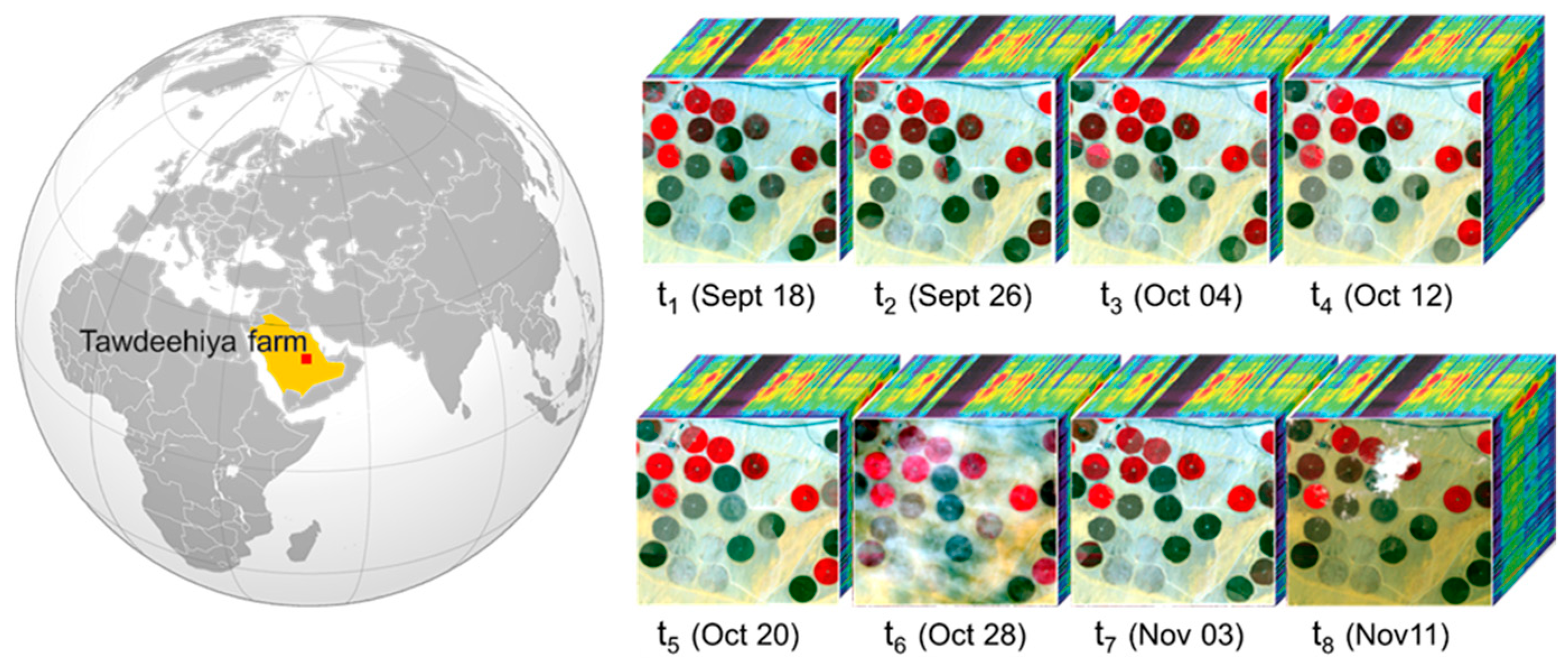
2.1. Study Site

The investigation was focused over the Tawdeehiya commercial farm, located around 70 km southeast of Al Kharj in Saudi Arabia. Situated in a flat desert environment, approximately 380 m above sea level, the farm covers around 30 km², growing a range of crops and vegetables across 47 center-pivots. The arid climate of this region is reflected by the 35 °C average daily maximum over the summer, and an average total annual precipitation of 90 mm, which is concentrated during the months of December through to April [34]. The site was chosen due to a range of ongoing hydrometeorological and remote sensing studies, which are supported by a dense network of ground-based infrastructure [35,36].

A sequence of Hyperion imagery was captured through the fall season from September 18 (DOY 261) to November 11 (DOY 315) 2015 (see Figure 1). Weather conditions during this period were characterized by an average daily maximum temperature of 30 °C, and an average daily low of 20 °C. Apart from the beginning of November, skies were mostly clear at the imagery collection time (09:00 UTC+3 approximately) [35]. Hazy conditions were frequently measured in MODIS aerosol optical thickness (AOT550) retrievals, indicating low visibility (see

Table 1. Scene collection conditions from the Hyperion metadata files.

Time (t)	Date	DOY	Time (UTC + 3)	Cloud (%)	AOD τ550	Visibility (km)	Sensor Azimuth (°)	Sensor Zenith (°)	Sensor Look Angle (°)
t1	18-Sep-15	261	8:54:05	2	0.405	18	112.475	153.778	26.222
t2	26-Sep-15	269	8:48:59	2	0.194	36	115.518	162.033	17.967
t3	4-Oct-15	277	8:43:00	2	0.366	20	118.321	171.426	8.5741
t4	12-Oct-15	285	8:37:22	4	0.460	16	120.731	181.554	-1.554
t5	20-Oct-15	293	8:31:39	4	0.564	13	122.827	168.255	11.745
t6	28-Oct-15	301	8:25:51	9	0.530	14	124.538	158.672	21.328
t7	3-Nov-15	307	8:45:51	4	0.490	15	130.147	159.946	20.054
t8	11-Nov-15	315	8:39:59	20	0.587	13	130.944	169.782	10.218

).

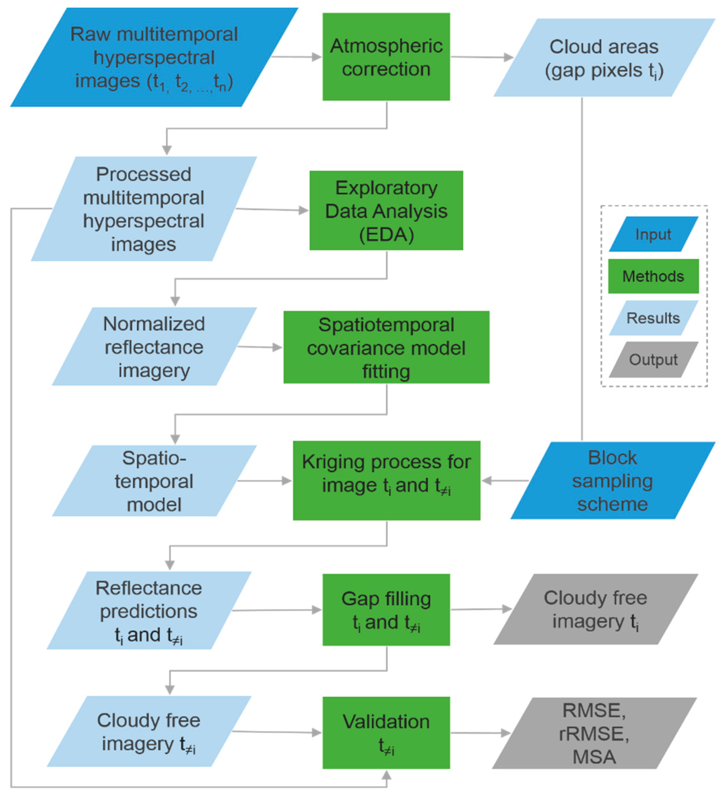
2.2. Hyperion Data Pre-Processing

Hyperion is a push-broom imager onboard the Earth Observing-1 (EO-1) satellite, and the first imaging system composed of two spectrometers in space. It records a total of 242 adjacent spectral channels, with one operating in the visible and near-infrared range (VNIR) between 400 and 1060 nm, and the other covering the shortwave infrared (SWIR) range between 860 and 2500 nm. Hyperion was programmed for targeted high-frequency collections in narrow swaths (7.5 km), with an off-nadir sensor viewing capability (±22°) that allows for up to five image acquisitions during a 16-day period over the same location [37]. Eight hyperspectral images captured over the study site were selected from the NASA-USGS Earth Explorer data pool. Each raw image includes 196 calibrated channels, with a spatial resolution of 30 m, 10 nm spectral resolution, and a cloud cover percentage of less than 10%. All scenes were radiometrically corrected to obtain absolute radiance (W·cm²·sr⁻¹·nm⁻¹) and pre-processed to eliminate bad bands before conversion from at-sensor radiance to surface reflectance. The Fast Line-of-sight Atmospheric Analysis of Spectral Hypercubes (FLAASH) tool in ENVI 5.1, which is based on the Moderate-resolution atmospheric transmission (MODTRAN) model [38], was used to perform the atmospheric correction. Water vapor was calculated using the U.S standard atmosphere model, setting water vapor absorption bands around 1135 nm, based on the non-tropical moisture conditions [39,40]. In addition, an aerosol optical depth at 550 nm was retrieved considering the standard MODTRAN maritime model. From Table 1, the 10 to 20 km visibility suggests the presence of larger particles. Here, the maritime aerosol is the best option since it gives a more realistic wavelength dependence and the desert model is not available in FLAASH. Visibility was estimated per scene via the Koschmieder Equation (1) [41], using aerosol optical depth (AOD) at 550 nm from the MOD04 product (see Table 1):

$$\mathrm{Visibility}=\frac{\ln \left(\frac{1}{\epsilon }\right)}{\left(E_{550}\right)+0.01159{\mathrm{km}}^{-1}},$$

(1)

where ε = 0.02 is the threshold contrast in MODTRAN, E_550 is the retrieved aerosol extinction coefficient at 550 nm, and 0.01159 km⁻¹ is the Rayleigh scattering coefficient for air at the surface at 550 nm. E550 is estimated by dividing AOD by an effective layer thickness of 2 km [40,41].

Since surface reflectance presents a large contrast in desert environments [42], there is an adjacency effect that mixes the reflectance/radiance spectra of the direct line-of-sight pixel with that of its neighboring pixels. In order to radiometrically compensate for this, FLAASH models adjacency effects through the convolution of the radiance image with a point spread function (PSF) kernel, also accounting for wavelength dependence and asymmetry in off-nadir viewing scenes [43]. PSF performs as an exponential function of the radial horizontal distance, depending on the aerosol scale height parameter used to calculate E₅₅₀ (2 km). Multiple scattering in short wavelengths (blue-red) is corrected by using the high-scatter DISORT model [44].

Previous noise assessments have reported a relatively low signal-to-noise ratio (SNR) in Hyperion data of different magnitudes in the VNIR and SWIR sensors [45,46], related to spatial and spectral artifacts, such as along-track stripping and smile effect in the cross-track direction. Removal of these effects was performed in two steps. First, enabling a FLAASH spectral polishing process [47], which consists of looking for some pixels whose spectra can be assumed as a smooth shape (for instance, bare soil free of spectral features and bright enough), and comparing their raw reflectance with a low-pass filtered spectrum to build a linear correction for the entire scene. Finally, a de-noising process was performed on each reflectance cube by running a minimum noise fraction (MNF) transformation [48], from which visible and near-infrared (VNIR) bands 8–57 (420 nm to 890 nm) together with short-wave infrared (SWIR) bands 77–120 (980 nm to 1350 nm), 130–165 (1440 nm to 1800 nm), and 181–222 (1950 nm to 2380 nm) were retained. This pre-processing resulted in a subset of the original cubes having 166 bands per scene.

Additionally, FLAASH defines a mask of cloudy pixels (cirrus and hazy) based on criteria, such as high albedo values, the amount of water in the column, and high reflectance in cirrus channels [49]. Each pixel of this mask is considered as a gap location to fill. The scene captured on November 11 was used as input data to calculate a mask that had an extent of 4 km² and covering a total of 4446 “cloud” pixels (Figure 1).

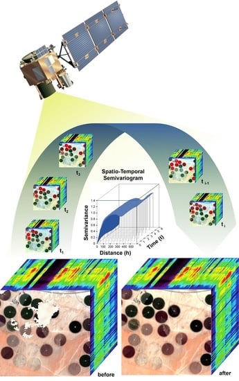
2.3. Spatiotemporal Statistics Approach

The aim of spatiotemporal statistical methods is to characterize a process by analyzing data sets and summarizing their main features in space and time. These techniques ensure that interpolation models produce realistic results in space and forecasts in time. In this research, the reflectance is assumed as a realization of a stochastic process for any hyperspectral datacube. Thus, a spatiotemporal regression model is implemented to estimate land surface reflectance at cloud affected locations in a Hyperion scene, producing a gap-filled image. From a multitemporal dataset of eight weekly collections covering the same area, the correlation between observations in space and time is used to fit a spatiotemporal covariance function and obtain predictions through kriging. The following sections describe the methodological workflow to sample, explore, and model the data, and ultimately the procedures used to evaluate the results. A schematic of this process is presented in Figure 2.

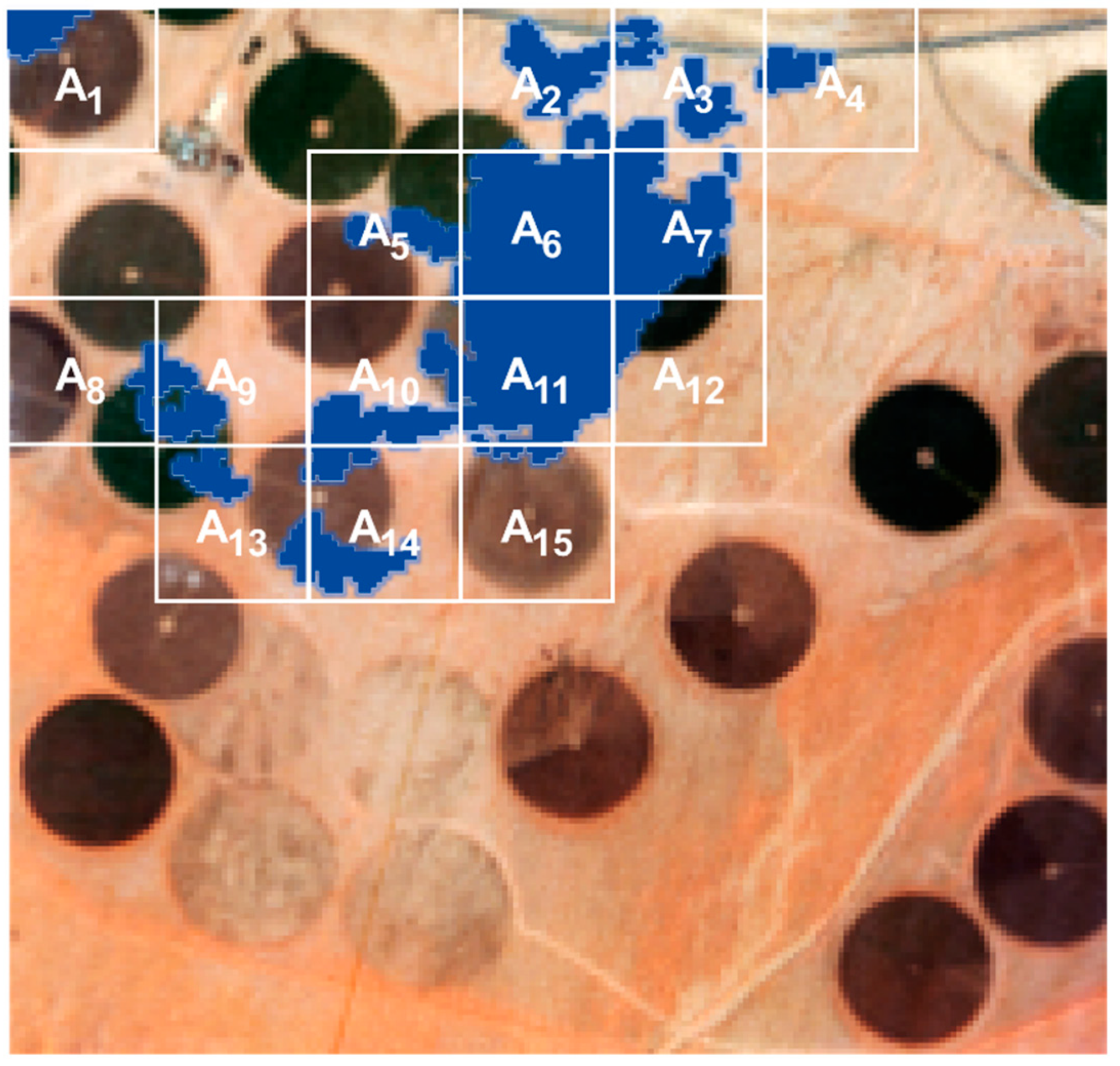
2.4. Block Sampling Scheme

Considering the size of the input hyperspectral dataset (210 rows x 210 columns x 166 bands x 8 times), an efficient sampling strategy is required to reduce the computational impact. The purpose of using a spatial sampling scheme is to collect representative training samples in the n-space domain to optimize parameter tuning in the model construction process [50]. One method to do this is stratified random sampling, under which the population is spatially divided into subgroups, which are non-overlapping, and whose subpopulation is independent and identically distributed while minimizing the heterogeneity in each group [51]. Following this, a strategy for simplifying the process is to divide the whole area covered by cloud masked pixels into several tiles and perform the prediction process for each of them separately, but parallelized. In this way, the sample statistics and uncertainty from this distribution can be incorporated in the kriging process [52]. Figure 3 shows the defined block scheme over the cloudy areas, which are divided into 15 polygons with dimensions of 30 × 30 pixels (see

Table 2. Cloud cover percentages per block.

Block	Clouds %	Block	Clouds %
A1	22	A9	25
A2	30	A10	28
A3	23	A11	90
A4	17	A12	18
A5	20	A13	20
A6	95	A14	32
A7	83	A15	5
A8	10

).

2.5. Spatiotemporal Covariance Function

The most important phase of the spatiotemporal prediction is choosing an appropriate covariance function to model the structure of the spatiotemporal variance of the data series. For this reason, statisticians are constantly seeking efficient and robust spatiotemporal covariance functions, and numerous parametric models have been proposed over the years [53]. Some of them, composed by means of the sum or product of purely spatial and purely temporal covariances, are referred to as separable functions. However, these are characterized by low flexibility and do not capture space–time interactions. Realizing these limitations, this paper follows an alternative type of covariance model called non-separable, which considers that a process can change dynamically, e.g., changes of land cover reflectance in space and over time. Under this approach, the reflectance is considered as a real-valued variable, Z(s,λ,t), observed at the coordinate triplets (s₁,λ₁,t₁),…,(s_i,λ_b,t_j), corresponding to the center point of a pixel at location s, band λ, and time t. It is assumed that Z(s,λ) has a mean function, μ(s,t) = E(Z(s,t)), and its covariance structure is stationary in space and time. Thus, Cov(Z(s,t),Z(s + h,t + u)) = C(h,u), where the covariance depends on the space and time lags, h and u. If u = 0, the covariance function, C(h,0), is purely spatial. Likewise, if h = 0, the covariance function, C(0,u), is considered purely temporal [54]. In contrast to separable models, non-separable functions have a different structure. One such example is that proposed by Gneiting (2) [55], which takes into account space-time interactions when h > 0 and u > 0:

$$C\left(h,u\right)=\frac{{\sigma }^2}{\psi {\left(\left|u^2\right|\right)}^{\frac{d}{2}}}\phi \left(\frac{\parallel h{\parallel }^2}{\psi ({\left|u\right|}^2)}\right),\left(h,u\right)\in {ℝ}^d\times ℝ,$$

(2)

where d = 2 (two dimensions), σ² is the variance of the process, φ(t) is any completely monotone function and represents the spatial structure of the covariance, and ψ(t) is any positive function with a completely monotonic derivative and represents the temporal structure of the covariance.

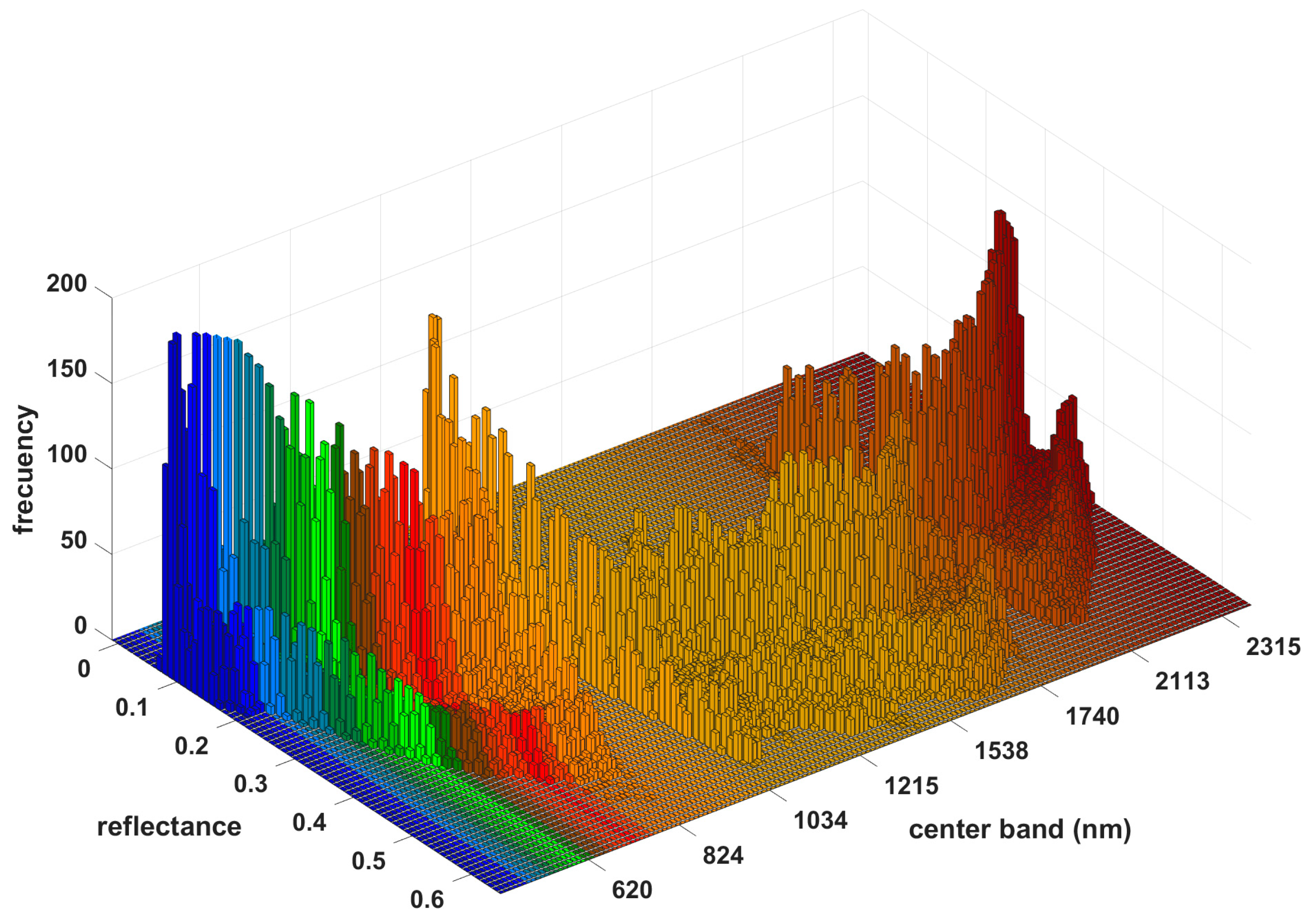
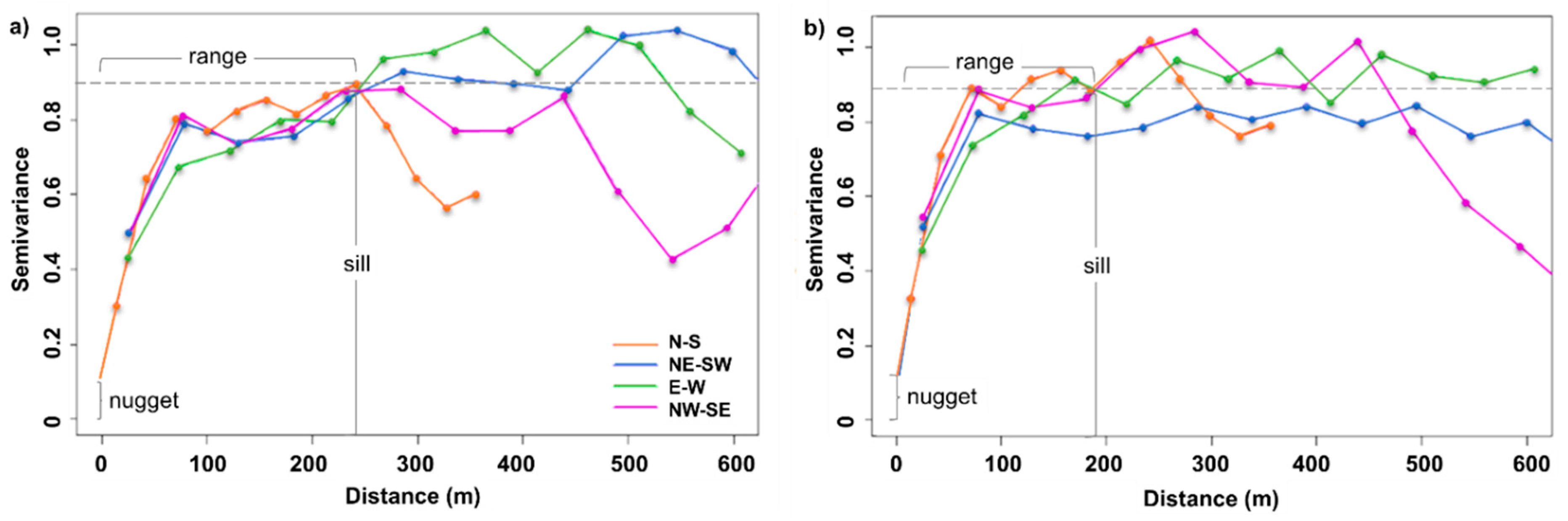
2.6. Exploratory Data Analysis

An exploratory data analysis is required to assess the assumptions on which the non-separable approach is based, which includes that the data is normally distributed, stationary, and correlated through time. If these conditions do not hold, then the covariance function is incorrectly fitted, which can result in inaccurate predictions. First, histograms were plotted to explore the reflectance distribution and homogeneity per band, based on clear-sky pixels only. Figure 4 shows an example of histograms for each band of one of the blocks delimited on the November 11 scene. In this example, most of the band-histograms are right or left skewed and do not represent normal distributions. If the empirical distribution is skewed, then the kriging estimator is likely to be sensitive to overestimation.

Transformation of data is commonly used to facilitate the modeling of non-Gaussian distributions under Gaussian assumptions [56]. One strategy is the standardization method (3), whereby values are adjusted for differing levels and spread using the mean and standard deviation of the variable:

$$Z^{*}=\frac{Z-\mu }{\sigma }.$$

(3)

Then, the resulting standardized reflectance, Z* (s,λ,t), is used as input for subsequent modeling. Figure 5 shows an example comparing the multitemporal distribution of a single band before and after the standardization. It is noticeable how the transformation changes the scale of the variable making all histograms comparable, centering them along a zero mean, μ*. An additional premise to verify is the second-order stationarity, which is based on two aspects: The mean is constant between samples at any location, and the covariance or semivariance is the same between any pair of points that are at the same distance and direction apart. To examine this, directional semivariograms per band were plotted to explore the spatial autocorrelation in the data and check for significant spatial trends. Each semivariogram results from measuring the distance between any two pixels and plotting the difference squared between the residual reflectance values at the sampled locations. An example of two different bands is presented in Figure 6, which shows the distance ranges reached by the four principal directional semivariograms, 180 m (see Figure 6b) in the case of band 23, and 240 m (see Figure 6a) for band 13. Their close trend indicates that variance behaves similarly in all directions before reaching the sill, thereby supporting the stationarity assumption.

Finally, the empirical temporal correlation was evaluated by estimating a multitemporal autocorrelation matrix for all datacubes based on a linear Pearson’s correlation. Autocorrelation refers to a variable which is correlated with itself. In this case, temporally-near images (i.e., close in time to each other) are more likely to have similar reflectance values and high correlation, while image pairs further apart in time are likely to have less similar values and low correlation. Figure 7 presents the high degree of temporal autocorrelation over an approximately 2 month period, and indicating that it is possible to predict a value at one specific time based on the values sampled (before or after) from a near-in-time scene.

2.7. Spatiotemporal Covariance Model Fitting and Kriging

After performing the exploratory data analysis, the standardized reflectance dataset is used as input to fit a parametric spatiotemporal variogram per band. A special case of the nonseparable and stationary covariance proposed by Gneiting (2) [55] is modeled using the package ‘CompRandFld’ (4) (5) (6), which was coded by Padoan and Bevilacqua [57] in R [58]:

$$C_{st}\left(h;u\right)=g_t{\left(u\right)}^{-1}\exp \left\{-\frac{d_s\left(h\right)}{g_t{\left(u\right)}^{-\frac{\eta k_s}{2}}}\right\},0\le \eta \le 1,$$

(4)

$$d_s\left(h\right)={\left(\frac{\parallel h\parallel }{{\psi }_s}\right)}^{k_s},g_s\left(h\right)=1+d_s\left(h\right),{\psi }_s,{\psi }_t>0,$$

(5)

$$d_t\left(u\right)={\left(\frac{\left|u\right|}{{\psi }_t}\right)}^{k_t},g_t\left(u\right)=1+d_t\left(u\right),0<k_s,k_t\le 2,$$

(6)

where $k_s$ and $k_t$ are smoothing parameters, ${\psi }_s$ and ${\psi }_t$ represent the scale parameters, with s and t subscripts representing space and time structures, respectively, and $\eta$ is the separability parameter that defines the spatiotemporal interaction of the variable, Z, taking values between 0 and 1. When $\eta =1$, the covariance model is considered non-separable. When $\eta =0$, this is considered separable. With the variable, Z, representing reflectance, as $\eta$ increases, the spatiotemporal interaction of the reflectance strengthens.

Once the empirical semivariograms are defined, the dataset is rearranged before performing the fitting process per band. Considering each one of the eight hyperspectral images as a 3D matrix, captured in time t, with s pixels and λ = 166 bands, these are reorganized into 166 individual 2D matrices by stacking the s pixels per band in a column and then joining the eight multitemporal single lines.

Several methods have been proposed to fit a semivariogram [59]. Here, the composite marginal likelihood (CML) is used for the joint optimization of the set of parameters formulated in Equations (4), (5), and (6). CML is an ideal likelihood fitting procedure in terms of computational efficiency for big datasets [60], since it does not require matrix inversions and is implemented in the R package. Likelihood refers to the probability that a given model could produce the observed data, with the likelihood function of the vector of parameters, θ = (η,k_s,k_t,ψ_s,ψ_t), given the observed data Z* = (Z*(s₁;t₁),…,Z*(s_i;t_j)) expressed as (7):

$$ℒ\left(\theta \right|Z\prime )=f\left(\theta ;Z^{*}\right).$$

(7)

The composite marginal case considers a likelihood based on only a part of the data, for example, by using each one of the blocks, $A_R$, previously defined (Figure 3) rather than a whole scene. If $A=\{A_1,\dots ,A_R\}$ is a marginal subset of $Z^{*}\left(s_i;t_j\right)$, with $i>R$, then the CML could be formulated as (8):

$$CML\left(\theta ;A_R\right)={{\displaystyle \sum }}_{r=1}^{R}f\left(\theta ;A_r\right),$$

(8)

whose composite estimator, ${\widehat{\theta }}_{CML}$, maximizes the probability of the parametrized model for each block of observed data (9):

$${\widehat{\theta }}_{CML}=arg\underset{\theta }{\max }CML\left(\theta ;A_R\right),CML\left({\widehat{\theta }}_{CML};A_R\right)\ge CML\left(\theta ;A_R\right).$$

(9)

The Akaike information criterion (AIC) is a metric used for the best model selection for the given data [61]. The model with the smallest AIC score is then the best fitting option (i.e., the one that minimizes the distance between the model and the truth values). It is defined here as (10):

$$AIC=-2CLM\left(\theta ;A_R\right)+2K,$$

(10)

where $K$ represents the number of parameters in the fitted model.

Three different separability scenarios are considered to evaluate the spatiotemporal interaction of the reflectance given the input data series when $\eta =\left\{0,0.5,1\right\}$. Once the best model is selected, each empirical semivariogram per band is fitted to the theoretical family function and is now ready to perform the spatiotemporal predictions. The selection of a Kriging method depends on the degree of stationarity followed by the process [62]. Here, the simple Kriging approach is used, since $Z^{*}$ follows a second-order stationarity with a constant and known mean ${\mu }^{*}$, and known covariance function, $C_{st}\left(h;u\right)$. Assuming that $Z^{*}$ is composed by the true process, $Y\left(s;t\right)$, and the measurement error, $\epsilon$, this could be denoted as (11):

$$Z^{*}=Y+\epsilon ,$$

(11)

where ε is a normally distributed measurement error with a mean, E(ε) = 0, and variance, var(ε) = σ_ε². If the aim is to predict the gap positions, Y($s$₀;t₀), for the image at time t₈ from the observed data, Z*, the simple Kriging predictor, $\widehat{Y}$, is defined as (12):

$$\widehat{Y}\left(s_0;t_o\right)={\mu }^{*}\left(s_0;t_0\right)+C_{st}{\left(s_0;t_0\right)}^{\prime }{C}_{st}^{-1}\left(Z^{*}\left(s_i;t_j\right)-{\mu }^{*}\left(s_i;t_j\right)\right).$$

(12)

Finally, after obtaining the kriged results, these are back-transformed to the units of the original data and replaced pixel by pixel and band by band, filling the cloud affected locations in the original hyperspectral scene (13):

$$\widehat{Z}=\widehat{Y}\sigma +\mu .$$

(13)

2.8. Evaluation of Results

The model is evaluated by imposing a sample cloud from the original mask (t₈) over four different free-cloud scenes, t₁, t₂, t₃, and t₄. The predictions are performed using a subset of three concentric blocks, in order to assess the accuracy of the model under high percentages of clouds, different block sizes, and different times. The defined sizes were 30 × 30 (area 1), 60 × 60 (area 2), and 90 × 90 (area 3) pixels, with 95%, 75%, and 55% of cloud cover levels, respectively (see Figure 8) (see

Table 3. Size and percentage of cloud pixels comprised by each area.

Block	Size	% of Clouds
Area 1	30 × 30	95
Area 2	60 × 60	75
Area 3	90 × 90	55

). Each round of evaluation involves masking one block per time and per band, then fitting the model using the cloud-free data series and retrieving the prediction on the subset of masked pixels.

Quantitative statistical metrics, such as the root mean square error (RMSE), the relative root mean squared error (rRMSE), and the mean spectral angle (MSA), were used to assess the performance of the model in estimating reflectance over these cloud-imposed areas. Since the kriging round is executed band by band for every single block, the RMSE (14) is used as a standard statistical metric to measure the model performance, by calculating the residuals between the predictions, $\widehat{Z}$, and true reflectance, Z, and aggregating the residuals into a single measure per band:

$$RMSE=\sqrt{\frac{1}{n}{{\displaystyle \sum }}_{i=1}^n{\left(\widehat{Z}\left(s_i;t_j\right)-Z\left(s_i;t_j\right)\right)}^2}.$$

(14)

One of the properties of RMSE is that it operates in the same units as the predicted variable. In this case, the unit of reflectance is percent (%), with possible values between 0 and 100. Thus, the closer the RMSE values are to zero, the more precise the interpolator. Considering that bands in the visible domain often have relatively lower reflectance than those in the near infrared region, a relative metric is reported in addition to the RMSE. The rRMSE (15) represents the root mean square error estimated as a percentage (%) of the mean measures, where lower values indicate less residual variance:

$$rRMSE=\sqrt{\frac{1}{n}{{\displaystyle \sum }}_{i=1}^n{\left(\widehat{Z}\left(s_i;t_j\right)-Z\left(s_i;t_j\right)\right)}^2}\ast \frac{100}{\overline{\frac{1}{n}{{\displaystyle \sum }}_{i=1}^{n}Z\left(s_i;t_j\right)}}.$$

(15)

The MSA (16) measures the spectral similarity between the predicted and the observed spectra [28]. By considering these as vectors in a space $b$-dimensional, the angle between them is calculated in a range from 0° (high similarity) to 90° (high dissimilarity). This metric is not affected by solar illumination effects since this is independent of the vectors length.

$$MSA=\frac{1}{n}\times \frac{180}{\pi }{{\displaystyle \sum }}_{i=1}^n{\cos }^{-1}\frac{{{\displaystyle \sum }}_{j=1}^{b}Z\left(s_i;{\lambda }_b;t_4\right)\widehat{Z}\left(s_i;{\lambda }_b;t_4\right)}{\sqrt{{{\displaystyle \sum }}_{j=1}^{b}Z{\left(s_i;{\lambda }_b;t_4\right)}^2{{\displaystyle \sum }}_{j=1}^b\widehat{Z}{\left(s_i;{\lambda }_b;t_4\right)}^2}}.$$

(16)

3. Results

As discussed above, the main goal of this study is to model the spatiotemporal correlation of surface reflectance to produce realistic predictions under cloud affected pixels in hyperspectral images. A general class of covariance functions was implemented to model the spatiotemporal features contained in a time series of hyperspectral imagery. As part of the processing workflow, model parameters were tuned following a likelihood-based criterion, and the best fitting covariance function was selected to perform the interpolation. The prediction results and the model evaluation over areas dominated by croplands, bare soil, and desert are presented in the following sections.

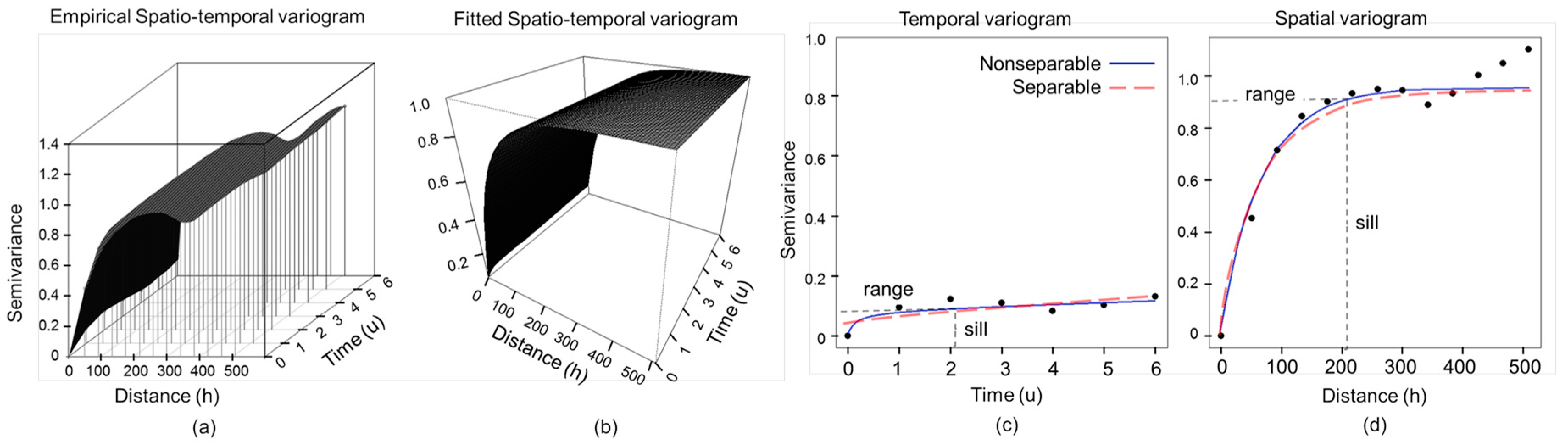
3.1. Spatiotemporal Covariance Model

For the cloudy scene, t₈, a spatiotemporal covariance function was fitted for predicting reflectance across cloud affected pixels. The sensitivity of the model was evaluated based on the separability, $\eta$, which is the only free-parameter, considering three different scenarios. In accordance with Gneiting [54], as $\eta$ increases, the space–time interaction strengthens.

Table 4. Fitted parameters and Akaike information criterion reported for three modeled scenarios.

Separability $\mathit{\eta }$	Power Space ${\mathit{k}}_{\mathit{s}}$	Power Time ${\mathit{k}}_{\mathit{t}}$	Scale Space ${\mathit{\psi }}_{\mathit{s}}$	Scale Time ${\mathit{\psi }}_{\mathit{t}}$	Spatial Sill	Temporal Sill	AIC
0	0.25	2	400	6	0.96	0.16	6330.44
0.5	1.50	1	290	4	0.93	0.11	6311.78
1	1.50	0.25	200	2	0.91	0.09	6305.72

presents the estimated parameters obtained by the composite maximum likelihood estimator.

The separable ($\eta =0$) and non-separable ($\eta =1$) cases are shown in Figure 9. Figure 9a displays a 3D cloud of points representing the empirical spatiotemporal variogram, where each column profile corresponds to a temporal variogram for a given spatial distance, and each row profile corresponds to a spatial variogram for a given temporal instant. Figure 9b shows the fitted version for the nonseparable case. Figure 9c,d show the temporal and spatial variogram, respectively. Points represent the empirical semivariance, and the red and blue lines the parametric estimates. Comparing these, it is noticeable how different power values (k_s,k_t) define the smooth fitting of the curve, and how the scale parameters define the ranges in time (ψ_t) and distance (ψ_s), where the models first flatten out to reach a sill. The lower AIC value reached by the last model in Table 4 (when $\eta =1$), suggests that the non-separable method performs the best fit, which means that for this dataset, a model that accounts for time–space interactions is suitable. Both spatial and temporal variograms provide information about how much two sampled pixels vary in reflectance percentage, depending on the distance and time between them. Following the spatial autocorrelation principle [53], pixels that are closer should have similar values, and as they become farther apart, they should be more dissimilar. In the case of boundary areas where two or more land cover types converge, the spatial autocorrelation will be low and the estimation will rely mostly on the temporal component of the model. At some distance and lapse of time, in this case, 200 meters and 2 weeks, the differences between pixels become fairly constant and the spatial and temporal variograms flattens out into a maximum variance of 0.91 and 0.09, respectively (see Figure 9b). This means that from 0 to 200 meters of spatial distance, and considering up to 2 weeks of temporal difference, the pixel reflectance can still be considered autocorrelated.

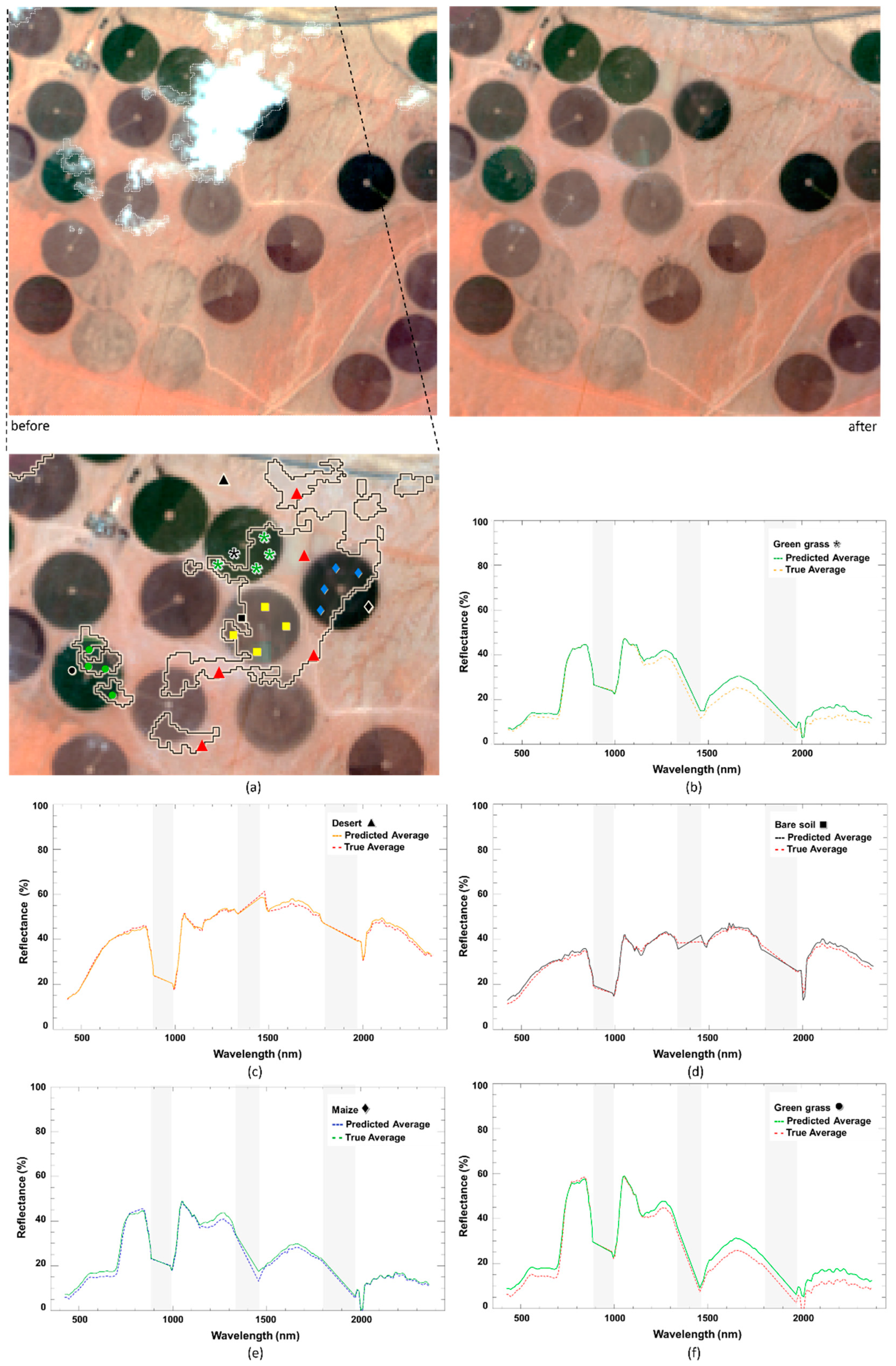
3.2. Reflectance Predictions

The fitted nonseparable covariance is used as input to perform simple kriging per block, and each band is processed by following the methodology described before. The gap positions are then filled with the predicted reflectance values, and all bands are stacked together in a single hyperspectral data cube to create the new cloud-free image. Figure 10 displays the image result for t₈ (top right panel), zooming in on the initial cloud affected area. A visual inspection of the results shows how cloudy areas with different shapes and sizes were filled with predicted reflectance values over heterogeneous land covers, including grass, maize (at maturity stage), bare-field soil, and desert soil. Clear spatial patterns and features in the original image are retained: For instance, the uniformity in circle pivot edges, the linear features of some trails, and the center pivot locations.

Figure 10b–f display a comparison between the averaged observed spectral profiles for each land cover type and the predicted spectral signatures across a selection of cloud affected pixels. Absorptions or minimum reflectance in spectra provide a good reference for analyzing the reconstruction results, since they reflect the unique spectral response to the land cover, or mixtures of covers, within each pixel. Of course, sometimes very different materials can be chemically and spectrally similar, resulting in comparable responses. Examining these spectra for each land cover specific case, the maize predicted profiles were similar to the reference signature, although an overestimation of approximately 4% of absolute reflectance was evident in the red absorption (550–700 nm) and in the near-infrared region (1180–1320 nm). The reconstructed profile for the desert soil presented a close match through the visible and near-infrared until 1450 nm, after which the predicted value exceeded the reference by approximately 3% of absolute reflectance in the 1500 to 1700 nm region and around 1% in the middle infrared. The bare soil response was similar in shape, but less reflective than the desert spectrum, with an approximately 8% lower predicted across all wavelengths. Finally, the Rhodes grass gap-filled predictions were overestimated for most of the bands by approximately 5% of absolute reflectance in the visible region, 3% between 1150 nm and 1320 nm, and 8% in the middle infrared bands. In all land cover specific cases, the shape of the predicted reflectance curves closely matched the observed image spectra, which indicates that the method works well in preserving the spectral consistency across wavelengths.

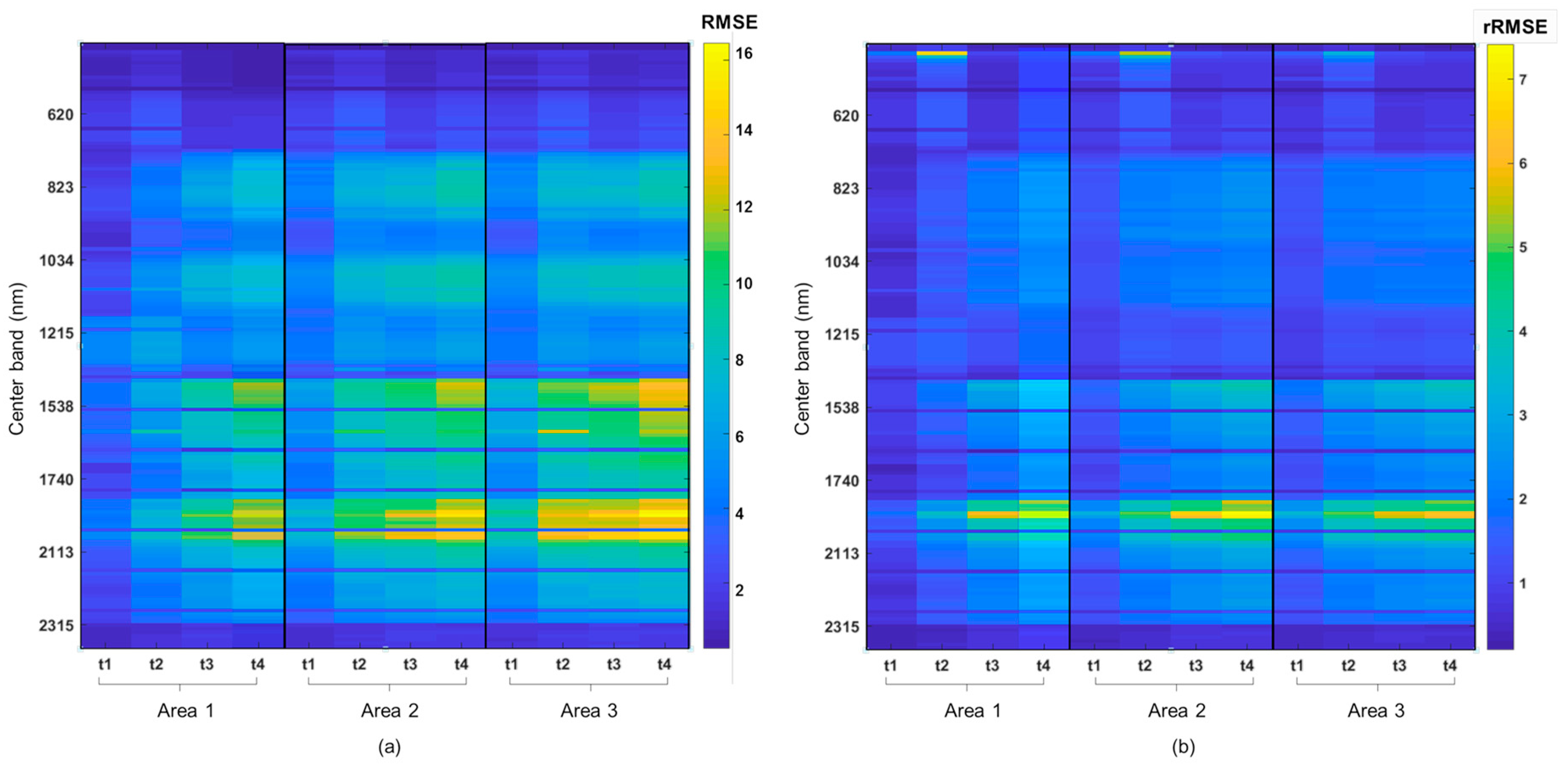
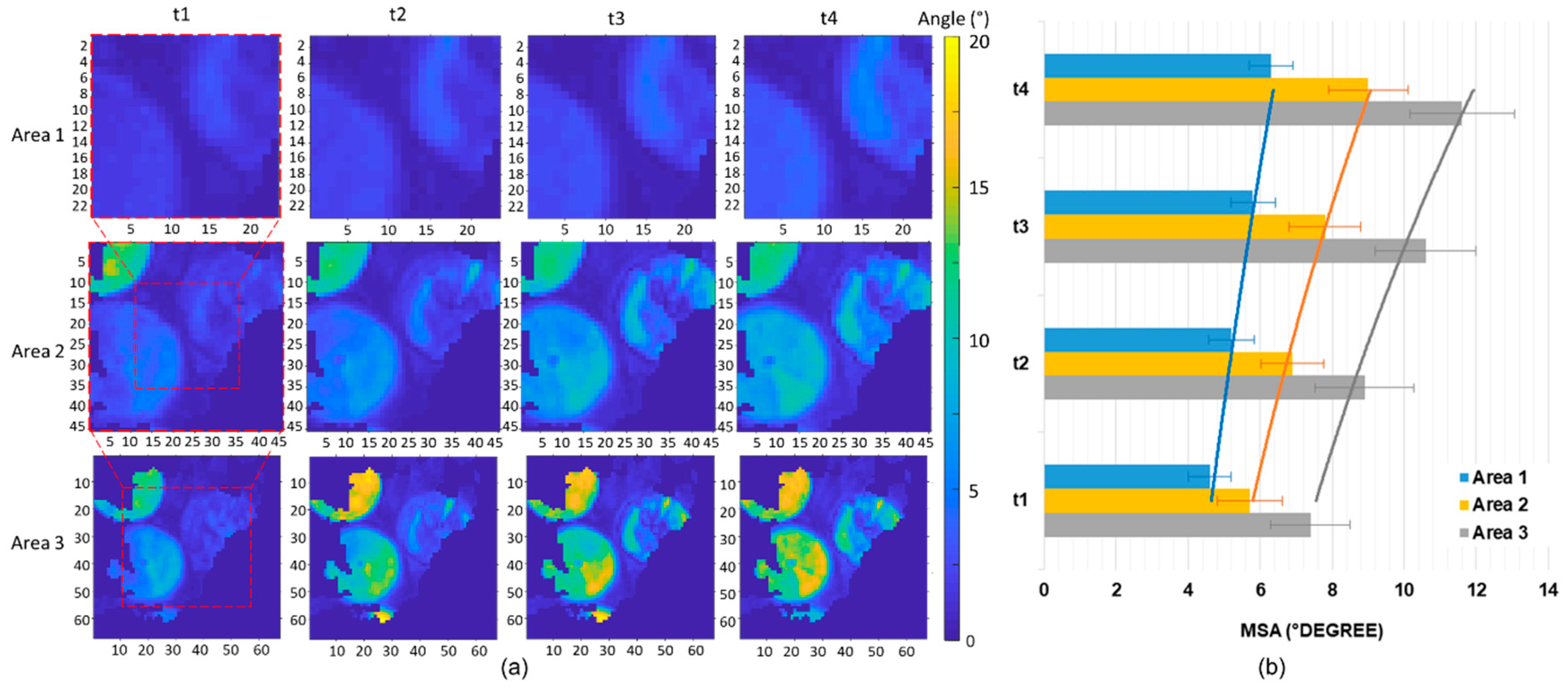
3.3. Evaluation of Cloud-Free Imagery

As described previously, the methodology was also evaluated using cloud-free areas from images t₁, t₂, t₃, and t₄, by superimposing an artificial cloud and performing the prediction on each one of these. Figure 11 presents the achieved root mean square error (RMSE) and relative root mean square error (rRMSE) per band (rows), for each time and sampled area (columns). As can be seen, low RMSE and rRMSE are achieved for most of the bands. Those in the visible spectrum from 420 to 700 nm and in the shortwave infrared from 2300 to 2350 nm, show the lowest RMSE values (0.5%–3% of absolute reflectance), which amount to an rRMSE of between 0.3% and 2%. In contrast, the largest RMSE (13%–16% of absolute reflectance) were estimated for shortwave infrared channels, corresponding to an rRMSE between 6% and 7% for those bands centered on 1500 nm, and between 3% and 4% for those centered on 2000 nm. It is evident that the accuracy of the model varies depending on the block size, but not on the cloud percentage, since there is an incremental RMSE as the block size grows while the cloud area decreases (Figure 8). Comparing the residual results in time, there is a slight incremental trend from t₁ to t₄ predictions, although that trend strengthens as the area size increases. For area 1, the minimum RMSE (0.5% of absolute reflectance) is achieved when t₁ is modeled, and the maximum RMSE of around 11% and 12% when t₄ is considered. For the larger prediction blocks (area 2 and area 3), higher residuals start to appear at a range of 13% to 14% and 14% to 16%, respectively. Consistent with the tendency observed in the RMSE, the prediction errors show overall low variances for the evaluated scenarios with some high rRMSE values for those bands centered on the 2000 nm wavelength (Figure 11b).

The spectral coherence of the results was assessed on the basis of the mean spectral angle (MSA) estimation conducted over the predicted pixels. Using this metric, the spectral similarity between the predicted and observed spectra was determined for each gap location (Figure 12a). As demonstrated in the residual analysis above, the block size can have a substantial impact on resulting surface reflectance predictions. The lowest MSA were achieved for the smallest test area, with spectral angles between 4° and 7°. For larger windows (i.e., area 2 and area 3), the spectral coherence is affected as time goes by, particularly for dynamic areas covered by pivot crops. Spectral differences ranging from 5 to 10° are obtained for area 2. The model produces comparatively higher MSA for area 3 (7, 9, 10.5, and 11.5°) (Figure 12b), consistent with the tendency observed in the other tiles. Overall, the high spectral similarity achieved for all the predicted pixel locations under the smallest tiling scheme indicates a satisfactory performance of the method to model the spatiotemporal dynamics of surface reflectance.

4. Discussion

Following is a more detailed examination of the proposed spatiotemporal gap-filling methodology, focusing on some of the challenges related to the spectral consistency of the results, and the performance of the sampling strategy under heterogeneous areas, and providing some guidance on improvements and future work required to improve the computational efficiency of the method.

4.1. Spatiotemporal Statistical Model for Predicting Reflectance

One of the motivations of this work was to exploit the spatial, temporal, and spectral information within this dataset to fit a spatiotemporal predictive model, and then to use this model to fill the missing data. An exploratory analysis provided a means to examine the data distribution and the spatial and temporal autocorrelation among the measured values, which are key considerations in determining how the interpolation model should be constructed. It was anticipated that the data would not follow a Gaussian distribution (Figure 5) since reflectance values vary according to the land surface dynamics. Thus, the data were transformed (Figure 6) to satisfy the normal distribution and stationarity assumptions required for kriging (Figure 7). Some authors [22,63] have suggested that these assumptions may limit the applicability of kriging approaches in remote sensing. However, this strategy is recognized as a useful tool to perform the interpolation, enabling the transformation of predictions back to their original scale [56]. Overall, the data was highly temporally autocorrelated, with a slight dependence on the time separation between scenes (Figure 9), indicating that temporally close images were more correlated to each other. However, since the data were collected weekly, and during a transition between summer and fall, the correlation for the last two scenes was only moderate.

Following the exploratory analysis, the critical stage of the prediction process was selecting and fitting the covariance function (Figure 9). In contrast to methods proposed by Zhang et al. and Pringle et al. [63,64] (

Table 5. Spatial and temporal statistical approaches for gap-filling remote sensing data.

Author	Covariance Function	Domains	Fitting Method	Kriging
Zhang et al. [61]	Exponential	Spatial (2D) + Temporal (1D)	Full likelihood	Ordinary, Co-Kriging
Pringle et al. [62]	Double spherical	Spatial (2D) + Temporal (1D)	Simulated annealing	Co-Kriging
Here proposed	Gneiting	Spatio-temporal (3D)	Composite marginal likelihood	Simple

), which model the spatial and temporal correlation separately by fitting two-dimensional covariance functions, here, we used a single three-dimensional model to account for the spatiotemporal autocorrelation of the measured sample pixels. The approach developed by Gneiting [55] was employed for its practicality, avoiding complex formulations and providing a general class of parametric spatiotemporal covariance functions. Comprised of seven unique parameters (three spatial, three temporal, and one for the structure separability), the approach was fitted in an automated way by using the composite marginal likelihood (CML) method. This provides an advantage over other solutions since in practice, fitting a semivariogram model is often done by eye, trying different parameter combinations based on the empirical variogram and running cross-validation to select the best model [65]. Such an approach would limit the use of geostatistical techniques for hyperspectral datasets, considering that the process must be iterated as many times as the number of bands. Hence, one of the benefits of using a general class of functions optimized with a maximum likelihood method is being able to individually fit a covariance per channel. An additional advantage of CML is that the method provided a selection criterion (AIC) of the model, with which the nonseparable covariance class was selected for performing the best fit for these data (see Table 2). This reaffirms that reflectance must be considered as a process that evolves in both space and time, rather than only considering its spatial distribution at a given time (purely spatial process), or its evolution over time at a given location (purely temporal process). Once the model is fitted, any kriging technique can be used to perform the interpolation band by band, as developed by Pringle et al. [64], assuming that the autocorrelation through space and time provides more information than the cross-correlation between bands. An extension of this work can be addressed by exploring cross-covariance functions for multivariate random fields based on the Gneiting approach [66,67], considering each band as an individual variate (e.g., using tools, such as the R package, CompRandFld [57]). Additional challenges relating to the stationarity assumption can be addressed using covariance models, also based on Gneiting’s work, that capture the non-stationarity in data (small-scale space-time variations) without involving many additional parameters [68].

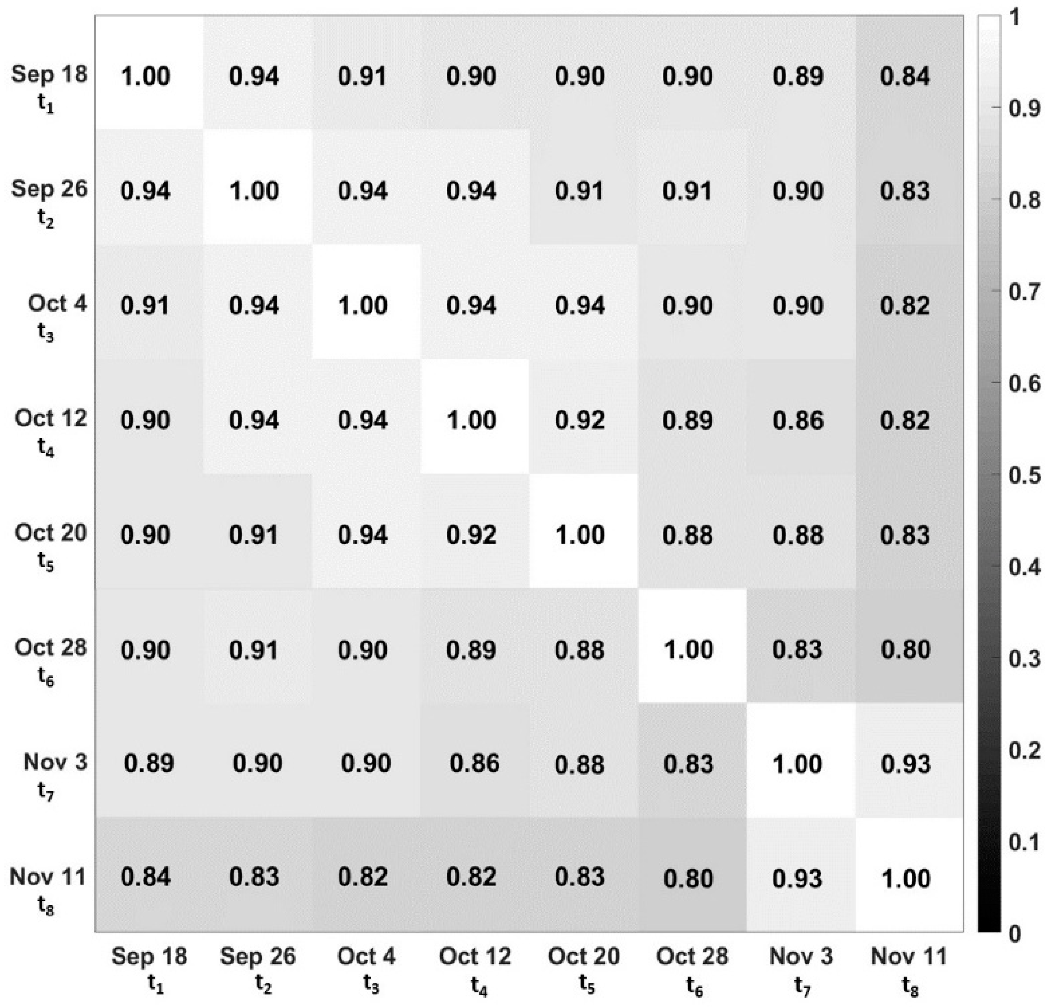
4.2. Assessment of the Spectral Consistency

One of the challenges in this study was to provide spectrally consistent predictions, which are required in numerous applications, such as thematic classification and change detection of land covers, or to monitor physical and chemical metrics of vegetation, bare soils, and water surfaces. The different land cover features present in the hyperspectral time-series were qualitatively and quantitatively analyzed to assess the spectral consistency of the results by comparing the predicted spectra with the observed signatures. In general, the predicted spectra were well matched to the real land cover types (Figure 10), achieving high levels of similarity across all the bands. Some slight systematic differences were evident between the visible (400 nm–700 nm) and near-infrared (700 nm–1300 nm) and the shortwave infrared (1300 nm–2300 nm) bands. From the prediction assessment over cloud-free areas, small and low variant residuals were obtained for the visible range, whereas higher residuals were achieved for the shortwave infrared bands (Figure 11). This wavelength-dependent effect could be related to a previously reported issue in the SWIR spectrometer of Hyperion [69], which presents a lower signal-to-noise ratio than the VNIR sensor and usually leads to calibration/registration issues in the SWIR bands. Although polishing and de-noising processes were performed on the raw data, some artifacts, like line striping, remained in these bands. However, this effect was not present in the VNIR bands, since the prediction was based on a band-by-band routine. To address this, some authors have suggested to process and model both datasets independently [70]. Figure 11a,b show this effect in both the RMSE and rRMSE results. Similarly, Figure 10b,f show how the same effect is even more evident in vegetation spectra, with slightly higher differences between the true and the predicted spectra, which is also noted in the MSA results (Figure 12). For further research in cross-covariance models attempting to exploit the correlation between bands, it is recommended to give attention to this kind of signal-to-noise mismatch between channels in order to avoid detrimentally affecting predictions.

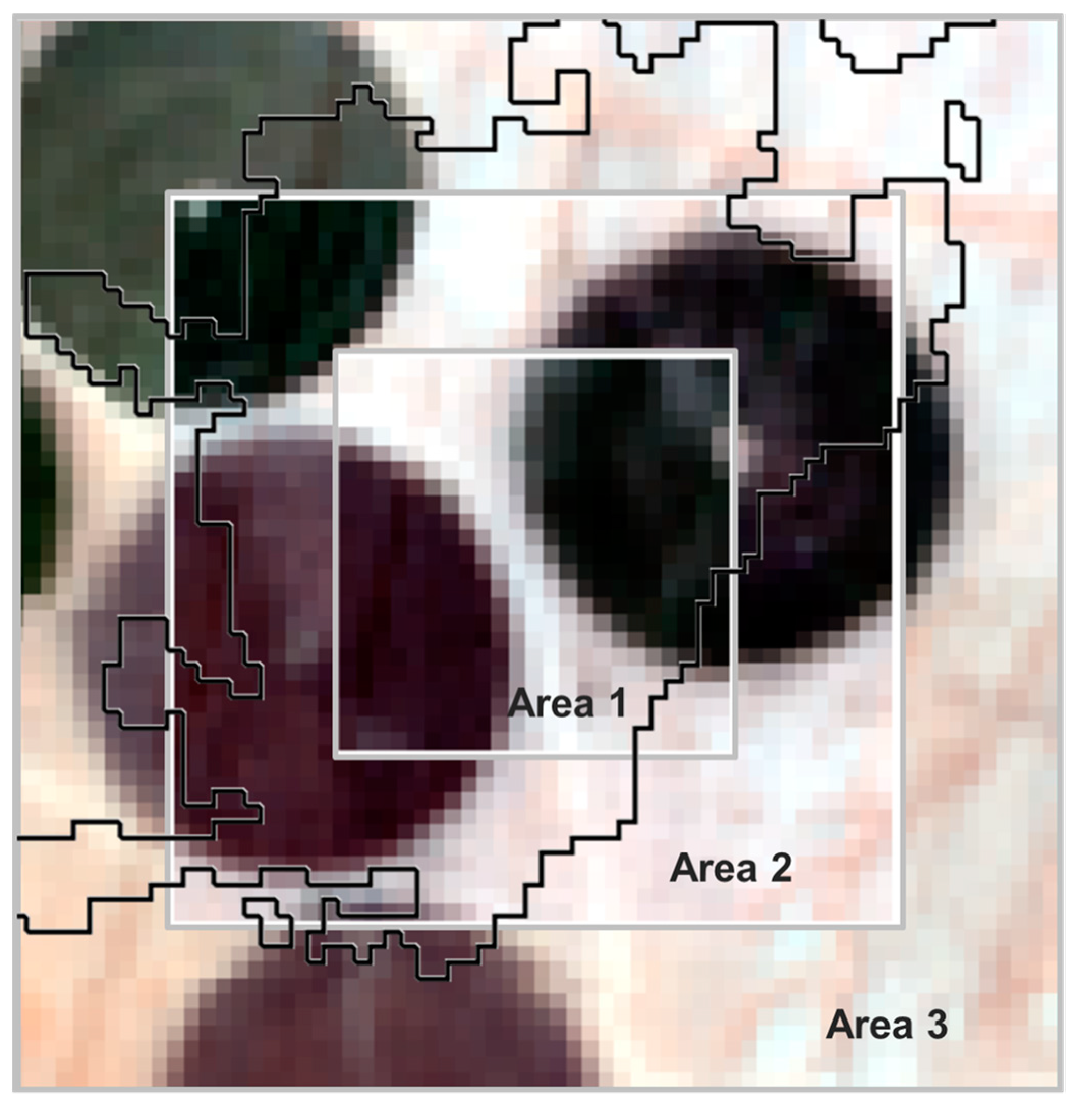
4.3. Block Sampling Strategy for Predictions in Heterogeneous Areas

The spatial sampling efficiency depends on the careful definition of shapes and size of the samples that capture the autocorrelation of the data [51]. Thus, all the spectral information from a sampled neighborhood is used to fit the covariance model. The blocking scheme, framed into the random stratified sampling, was efficient in selecting a subset of heterogeneous pixels within the cloud affected areas to capture representative sample statistics of the whole scene, thereby allowing the prediction of reflectance values at unsampled locations with minimum error variance. Other designs, like those based on the zonation of land covers [22], were not considered since it has been demonstrated that the efficiency of the prediction process is diminished and computationally expensive under highly dynamic data series [51]. Following the blocking strategy, the spatiotemporal and spectral consistency of the predictions was assessed, based on the grid size, the percentage of cloud cover, and time range. The error variation of predictions was minimal between blocks (Figure 11 and Figure 12) with slight variations in RMSE and MSA for bigger block sizes (area 2 and area 3). It should be stressed that even for high cloud percentages (i.e., area 1 with 95%), low errors and high spectrally coherent results were achieved. This suggests that the block sampling strategy should be implemented to only account for the observations close to the target gaps, by defining the block size based on the effective range from the empirical spatial variogram. Following the same rationale, the model should be used to gap fill data series based on temporally closer images, by determining the temporal range from the empirical temporal variogram. Additional further studies should be conducted over different larger areas where sampling blocks can include several dynamic cover types, and different grid sizes can be fitted according to the heterogeneity of a particularly targeted gap.

4.4. Computational Efficiency

Hyperspectral data can be difficult and computationally intensive to process, and both the sampling strategy and the quality of the data may affect the fidelity of the prediction process. Given the high spectral resolution of the dataset, the computational efficiency of the prediction process was a key concern in this study. This was addressed in two steps: 1) By defining the block sampling strategy, the number of pixels being processed at any one time is reduced significantly; and 2) by employing the CML estimator, which is considered as one of the fastest likelihood-based methods [57], to optimize the parametric estimation when fitting the covariance model. The prediction method required a wall time of 3 minutes for a datacube of 30 × 30 × 166 affected pixels, based on a complete iteration of the coded routine in R software, using a machine with a 3.4 GHz processor and 24 GB of memory. Further research should explore improvements in the kriging interpolator, which involves the inversion of covariance matrices with a high computational cost. Techniques, such as the fixed rank kriging (FRK) proposed by Cressie et al. [71], address the problems of both data size and spatial heterogeneity, while reducing the computational complexity of the conventional kriging formulation, and may provide an improvement in computational time.

5. Conclusions

The use of remotely sensed time series data for earth and environmental science applications are routinely constrained by the availability of cloud-free scenes. A wide range of gap-filling approaches has been developed to reconstruct cloud affected pixels, with geostatistical methods generally proving to be the most effective. However, few of these available techniques have examined their application to hyperspectral imagery as compared to multispectral data. Here, we exploited a prediction approach that is based on state-of-the-art spatiotemporal statistical modeling. From the wide range of valid covariance functions available, Gneiting’s method provides a flexible strategy to model surface reflectance as a physically dynamic process through time. Commonly used correlation functions in gap-filling and image denoising techniques often turn to generalizations of spatial statistical models to separately account for spatial and temporal features. Here, we proposed to address the limitations and complexity of separate modeling by implementing this novel spatiotemporal approach. To do this, space-time dynamics from a series of eight Hyperion scenes were modeled efficiently by fitting a single composed covariance function from which the gap-filling was processed by retrieving kriging predictions for cloud-masked locations. A block sampling technique was proposed to reduce the number of pixels to be processed at a time, and the use of a composite likelihood method improved the speed of the parameter estimation. Both strategies positively impacted the operability of the full workflow.

Overall, the predicted spectra achieved relatively low error residuals and high spectral similarity to reference signatures across a range of different land covers, preserving visual features, like shapes, textures, edges, and spatial continuity. A small systematic difference in the accuracy of the predicted reflectance between the VNIR and SWIR bands was attributed to the low signal-to-noise ratio of the Hyperion SWIR spectrometer, which has been previously reported in the literature. The spatial and spectral consistency of these results demonstrates the convenient use of spatiotemporal methods in image processing. Importantly, this approach can be extended to solve other gap-filling challenges in multi-temporal series of hyperspectral or multispectral images, such as shadows, dust, salt and pepper noise, orbit related missing data, and bright spots. Considering the increasing demand for realistic and computationally efficient solutions to model large remote sensing datasets, identifying novel and efficient approaches for producing high-quality time series and understanding land cover dynamics represents a much-needed focus of research.

References

1. Gamon, J.A.; Qiu, H.; Sanchez-Azofeifa, A. Ecological applications of remote sensing at multiple scales. In Functional Plant Ecology, 2nd ed.; Pugnaire, F., Valladares, F., Eds.; CRC Press: Boca Raton, FL, USA, 2007; Volume 1, pp. 655–675. [Google Scholar]
2. Ustin, S.L.; Gamon, J.A. Remote sensing of plant functional types. New Phytol. 2010, 186, 795–816. [Google Scholar] [CrossRef] [Green Version]
3. Malenovský, Z.; Mishra, K.; Zemek, F.; Rascher, U.; Nedbal, L. Scientific and technical challenges in remote sensing of plant canopy reflectance and fluorescence. J. Exp. Bot. 2009, 60, 2987–3004. [Google Scholar] [CrossRef] [Green Version]
4. Dale, L.; Thewis, A.; Boudry, C.; Rotar, L.; Dardenne, P.; Baeten, V.; Fernández, J.A. Hyperspectral imaging applications in agriculture and agro-food product quality and safety control: A review. Appl. Spectrosc. Rev. 2013, 48, 142–159. [Google Scholar] [CrossRef]
5. Preliminary Assessment of the Value of Landsat 7 ETM+ SLC-off Data. Available online: https://landsat.usgs.gov/sites/default/files/documents/SLC_off_Scientific_Usability.pdf (accessed on 8 April 2019).
6. Tanre, D.; Deschamps, P.Y.; Devaux, C.; Herman, M. Estimation of Saharan aerosol optical thickness from blurring effects in thematic mapper data. J. Geophys. Res. 1988, 93, 15955–15964. [Google Scholar] [CrossRef]
7. Adler-Golden, S.M.; Robertson, D.C.; Richtsmeier, S.C.; Ratkowski, A.J. Cloud effects in hyperspectral imagery from first-principles scene simulations. In Proceedings of the SPIE Defense, Security, and Sensing, Orlando, FL, USA, 27 April 2009. [Google Scholar]
8. Validation of On-Board Cloud Cover Assessment Using EO-1. Available online: https://eo1.gsfc.nasa.gov/new/extended/sensorWeb/EO-1_Validation On-board Cloud Assessment_Rpt.pdf (accessed on 8 April 2019).
9. Ju, J.; Roy, D.P. The availability of cloud-free Landsat ETM Plus data over the conterminous United States and globally. Remote Sens. Environ. 2007, 112, 1196–1211. [Google Scholar] [CrossRef]
10. Lin, C.H.; Tsai, P.H.; Lai, K.H.; Chen, J.Y. Cloud removal from multitemporal satellite images using information cloning. IEEE Trans. Geosci. Remote Sens. 2013, 51, 232–241. [Google Scholar] [CrossRef]
11. Shen, H.; Xinghua, L.; Cheng, Q.; Zeng, C.; Yang, G.; Li, H.; Zhang, L. Missing Information Reconstruction of Remote Sensing Data: A Technical Review. IEEE Geosci. Remote Sens. Mag. 2015, 3, 61–85. [Google Scholar] [CrossRef]
12. Helmer, E.; Ruefenacht, B. Cloud-free satellite image mosaics with regression trees and histogram matching. Photogramm. Eng. Remote Sens. 2005, 71, 1079–1089. [Google Scholar] [CrossRef]
13. Benabdelkader, S.; Melgani, F. Contextual spatiospectral postreconstruction of cloud-contaminated images. IEEE Geosc. Remote Sens. 2008, 5, 204–208. [Google Scholar] [CrossRef]
14. Melgani, F. Contextual reconstruction of cloud-contaminated multitemporal multispectral images. IEEE Trans. Geosci. Remote Sens. 2006, 44, 442–455. [Google Scholar] [CrossRef]
15. Shen, H.; Wu, J.; Cheng, Q.; Aihemaiti, M.; Zhang, C.; Li, Z. A spatiotemporal fusion based cloud removal method for remote sensing images with land cover changes. IEEE J. Sel. Top. Appl. Earth Obs. Remote Sens. 2019, 12, 862–874. [Google Scholar] [CrossRef]
16. Chang, N.B.; Bai, K.; Chen, C.F. Smart information reconstruction via time-space-spectrum continuum for cloud removal in satellite images. IEEE J. Sel. Top. Appl. Earth Obs. Remote Sens. 2015, 8, 1898–1912. [Google Scholar] [CrossRef]
17. Wang, B.; Ono, A.; Muramatsu, K.; Fujiwarattt, N. Automated detection and removal of clouds and their shadows from Landsat TM images. IEICE Trans. Inf. Syst. 1999, 82, 453–460. [Google Scholar]
18. Gabarda, S.; Cristóbal, G. Cloud covering denoising through image fusion. Image Vis. Comput. 2007, 25, 523–530. [Google Scholar] [CrossRef] [Green Version]
19. Roerink, G.J.; Menenti, M.; Verhoef, W. Reconstructing cloudfree NDVI composites using Fourier analysis of time series. Int. J. Remote Sens. 2010, 21, 1911–1917. [Google Scholar] [CrossRef]
20. Mariethoz, G.; McCabe, M.F.; Renard, P. Spatiotemporal reconstruction of gaps in multivariate fields using the direct sampling approach. Water Resour. Res. 2012, 48, W10507. [Google Scholar] [CrossRef]
21. Jha, S.K.; Mariethoz, G.; Evans, J.P.; McCabe, M.F. Demonstration of a geostatistical approach to physically consistent downscaling of climate modeling simulations. Water Resour. Res. 2013, 49, 245–259. [Google Scholar] [CrossRef] [Green Version]
22. Zhang, C.; Li, W.; Travis, D.J. Restoration of clouded pixels in multispectral remotely sensed imagery with cokriging. Int. J. Remote Sens. 2009, 30, 2173–2195. [Google Scholar] [CrossRef]
23. Meng, Q.M.; Borders, B.E.; Cieszewski, C.J.; Madden, M. Closest spectral fit for removing clouds and cloud shadows. Photogramm. Eng. Remote Sens. 2009, 75, 569–576. [Google Scholar] [CrossRef]
24. Cheng, Q.; Shen, H.; Zhang, L.; Yuan, Q.; Zeng, C. Cloud removal for remotely sensed images by similar pixel replacement guided with a spatio-temporal MRF model. ISPRS J. Photogramm. Remote Sens. 2014, 92, 54–68. [Google Scholar] [CrossRef]
25. Cerra, D.; Müller, R.; Reinartz, P. Cloud removal in image time series through unmixing. In Proceedings of the 8th International Workshop on the Analysis of Multitemporal Remote Sensing Images, Annecy, France, 22–24 July 2015. [Google Scholar]
26. Xu, M.; Pickering, M.; Plaza, A.J.; Jia, X. Thin cloud removal based on signal transmission principles and spectral mixture analysis. IEEE Trans. Geosci. Remote Sens. 2016, 54, 1659–1669. [Google Scholar] [CrossRef]
27. Feng, W.; Chen, Q.; He, W.; Gu, G.; Zhuang, J.; Xu, S. A defogging method based on hyperspectral unmixing. Acta Opt. Sin. 2015, 35, 115–122. [Google Scholar]
28. Yin, G.; Mariethoz, G.; McCabe, M.F. Gap-filling of landsat 7 imagery using the direct sampling method. Remote Sens. 2017, 9, 12. [Google Scholar] [CrossRef]
29. Shekhar, S.; Jiang, Z.; Ali, R.Y.; Eftelioglu, E.; Tang, X.; Gunturi, V.M.V.; Zhou, X. Spatiotemporal data mining: A computational perspective. ISPRS Int. J. Geo-Inf. 2015, 4, 2306–2338. [Google Scholar] [CrossRef]
30. Gneiting, T.; Genton, M.G.; Guttorp, P. Geostatistical space-time models, stationarity, separability and full symmetry. In Statistical Methods for Spatio-Temporal Systems, 1st ed.; Finkenstadt, B., Held, L., Isham, V., Eds.; Chapman and Hall/CRC: New York, NY, USA, 2006; Volume 1, pp. 151–175. [Google Scholar]
31. De Iaco, S.; Palma, M.; Posa, D. A general procedure for selecting a class of fully symmetric space-time covariance functions. Environmetrics 2016, 27, 212–224. [Google Scholar] [CrossRef]
32. Omidi, M.; Mohammadzadeh, M. A new method to build spatio-temporal covariance functions: Analysis of ozone data. Stat. Pap. 2015, 57, 689–703. [Google Scholar] [CrossRef]
33. De Iaco, S.; Myers, D.E.; Posa, D. Nonseparable space-time covariance models: Some parametric families. Math. Geol. 2002, 34, 23–42. [Google Scholar] [CrossRef]
34. Historical Weather for 2015 in Al-Kharj Prince Sultan Air Base, Saudi Arabia. WeatherSpark, 2015. Available online: http://weatherspark.com/history/32768/2015/Al-Kharj-Riyadh-Saudi-Arabia (accessed on 8 April 2019).
35. Houborg, R.; McCabe, M.F. Adapting a regularized canopy reflectance model (REGFLEC) for the retrieval challenges of dryland agricultural systems. Remote Sens. Environ. 2016, 186, 105–112. [Google Scholar] [CrossRef]
36. El Kenawy, A.M.; McCabe, M.F. A multi-decadal assessment of the performance of gauge and model based rainfall products over Saudi Arabia: Climatology, anomalies and trends. Int. J. Climatol. 2016, 36, 656–674. [Google Scholar] [CrossRef]
37. Folkman, M.A.; Pearlman, J.; Liao, L.B.; Jarecke, P.J. EO-1/Hyperion hyperspectral imager design, development, characterization, and calibration. Proc. SPIE 2001, 4151, 40–51. [Google Scholar] [Green Version]
38. Perkins, T.; Adler-Golden, S.M.; Matthew, M.W. Speed and accuracy improvements in FLAASH atmospheric correction of hyperspectral imagery. Opt. Eng. 2012, 51, 111707. [Google Scholar] [CrossRef]
39. Felde, G.W.; Anderson, G.P.; Gardner, J.A.; Adler-Golden, S.M.; Matthew, M.W.; Berk, A. Water vapor retrieval using the FLAASH atmospheric correction algorithm. In Proceedings of the SPIE Defense and Security, Orlando, FL, USA, 12 August 2004. [Google Scholar]
40. Rochford, P.; Acharya, P.; Adler-Golden, S.M. Validation and refinement of hyperspectral/multispectral atmospheric compensation using shadowband radiometers. IEEE Trans. Geosci. Remote Sen. 2005, 43, 2898–2907. [Google Scholar] [CrossRef]
41. Griffin, M.K.; Burke, H.K. Compensation of hyperspectral data for atmospheric effects. Linc. Lab. J. 2003, 14, 29–54. [Google Scholar]
42. Houborg, R.; McCabe, M.F. Impacts of dust aerosol and adjacency effects on the accuracy of Landsat 8 and RapidEye surface reflectances. Remote Sens. Environ. 2017, 194, 127–145. [Google Scholar] [CrossRef]
43. Adler-Golden, S.M.; Matthew, M.W.; Berk, A.; Fox, M.J.; Ratkowski, A.J. Improvements in aerosol retrieval for atmospheric correction. In Proceedings of the IGARSS 2008—2008 IEEE International Geoscience and Remote Sensing Symposium, Boston, MA, USA, 7–11 July 2008. [Google Scholar]
44. Stamnes, K.; Tsay, S.C.; Wiscombe, W.; Jayaweera, K. Numerically stable algorithm for Discrete-Ordinate-Method Radiative Transfer in multiple scattering and emitting layered media. Appl. Opt. 1988, 27, 2502–2509. [Google Scholar] [CrossRef]
45. Staenz, K.; Neville, R.A.; Clavette, S.; Landry, R.; White, H.P. Retrieval of surface reflectance from Hyperion radiance data. In Proceedings of the IEEE International Geoscience and Remote Sensing Symposium, Toronto, ON, Canada, 24–28 June 2002. [Google Scholar]
46. Pearlman, J.S.; Barry, P.S.; Segal, C.C.; Shepanski, J.; Beiso, D.; Carman, S.L. Hyperion, a space-based imaging spectrometer. IEEE Trans. Geosci. Remote Sens. 2003, 41, 1160–1173. [Google Scholar] [CrossRef]
47. Matthew, M.W.; Adler-Golden, S.M.; Berk, A.; Felde, G.; Anderson, G.P.; Gorodetzkey, D.; Paswaters, S.; Shippert, M. Atmospheric correction of spectral imagery: Evaluation of the FLAASH algorithm with AVIRIS data. In Proceedings of the Applied Imagery Pattern Recognition Workshop, Washington, DC, USA, 17–23 October 2003. [Google Scholar]
48. Green, A.A.; Berman, M.; Switzer, P.; Craig, M.D. A Transform for ordering multispectral data in terms of image quality with implications for noise removal. IEEE Int. Geosci. Remote Sens. 1988, 26, 65–74. [Google Scholar] [CrossRef]
49. Matthew, M.W.; Adler-Golden, S.M.; Berk, A.; Richtsmeier, S.C.; Levine, R.Y.; Bernstein, L.S.; Acharya, P.K.; Anderson, G.P.; Felde, G.W.; Hoke, M.P.; et al. Status of atmospheric correction using a modtran4-based algorithm. In Proceedings of the SPIE AeroSense 2000, Orlando, FL, USA, 23 August 2000. [Google Scholar]
50. Cochran, W.G. Sampling Techniques, 3rd ed.; John Wiley & Sons: New York, NY, USA, 1977. [Google Scholar]
51. Wang, J.F.; Haining, R.P.; Cao, Z.D. Sample surveying to estimate the mean of a heterogeneous surface: Reducing the error variance through zoning. Int. J. Geogr. Inf. Sci. 2010, 24, 523–543. [Google Scholar] [CrossRef]
52. Wang, J.F.; Stein, A.; Gao, B.; Ge, Y. A review of spatial sampling. Spat. Stat. 2012, 2, 1–14. [Google Scholar] [CrossRef]
53. Montero, J.M.; Fernández, G.; Mateu, J. Spatial and Spatio-Temporal Geostatistical Modeling and Kriging, 1st ed.; John Wiley & Sons: Chichester, UK, 2015; pp. 178–265. [Google Scholar]
54. Cressie, N.; Huang, H. Classes of nonseparable, spatio-temporal stationary covariance functions. J. Am. Stat. Assoc. 1999, 94, 1330–1340. [Google Scholar] [CrossRef]
55. Gneiting, T. Nonseparable, stationary covariance functions for space-time data. J. Am. Stat. Assoc. 2002, 97, 590–600. [Google Scholar] [CrossRef]
56. Tukey, J. On the comparative anatomy of transformations. Ann. Math. Stat. 1957, 28, 602–632. [Google Scholar] [CrossRef]
57. Package CompRandFld. R Package Version 1.0.3-4. Available online: https://cran.r-project.org/package=CompRandFld (accessed on 8 April 2019).
58. R Core Team. R: A Language and Environment for Statistical Computing. R Package Version 3.2.2. Available online: http://www.R-project.org (accessed on 8 April 2019).
59. Zimmerman, D.L.; Zimmerman, M.B. A comparison of spatial semivariogram estimators and corresponding ordinary kriging predictors. Technometrics 1991, 33, 77–91. [Google Scholar] [CrossRef]
60. Curriero, F.; Lele, S. A Composite Likelihood Approach to Semivariogram Estimation. J. Agric. Biol. Environ. Stat. 1999, 4, 9–28. [Google Scholar] [CrossRef]
61. Padoan, S.; Bevilacqua, M. Analysis of random fields using CompRandFld. J. Stat. Softw. 2015, 63, 1–27. [Google Scholar] [CrossRef]
62. Cressie, N.; Wikle, C. Statistics for Spatio-Temporal Data, 1st ed.; John Wiley & Sons: Chichester, UK, 2011. [Google Scholar]
63. Zhang, C.; Li, W.; Travis, D. Gaps-fill of SLC-off Landsat ETM+ satellite image using a geostatistical approach. Int. J. Remote Sens. 2007, 28, 5103–5122. [Google Scholar] [CrossRef]
64. Pringle, M.J.; Schmidt, M.; Muir, J.S. Geostatistical interpolation of SLC-off Landsat ETM+ images. ISPRS J. Photogramm. Remote Sens. 2009, 64, 654–664. [Google Scholar] [CrossRef]
65. Webster, R.; Oliver, M.A. Geostatistics for Environmental Scientists, 1st ed.; John Wiley & Sons: Chichester, UK, 2007. [Google Scholar]
66. Porcu, E.; Bevilacqua, M.; Genton, M. Spatio-temporal covariance and cross-covariance functions of the great circle distance on a sphere. J. Am. Stat. Assoc. 2016, 111, 888–898. [Google Scholar] [CrossRef]
67. Genton, M.; Kleiber, W. Cross-covariance functions for multivariate geostatistics. Stat. Sci. 2015, 30, 147–163. [Google Scholar] [CrossRef]
68. Jun, M. Non-stationary cross-covariance models for multivariate processes on a globe. Scand. J. Stat. 2011, 38, 726–747. [Google Scholar] [CrossRef]
69. Thome, K.J.; Biggar, S.F.; Wisniewski, W. Cross comparison of EO-1 sensors and other Earth resources sensors to Landsat-7 ETM+ using Railroad Valley Playa. IEEE Trans. Geosci. Remote Sens. 2003, 41, 1180–1188. [Google Scholar] [CrossRef]
70. Datt, B.; Jupp, D.L.B. Hyperion Data Processing Workshop, Hands-On Processing Instructions; CSIRO Office of Space Science & Applications Earth Observation Centre: Canberra, Australia, 2004. [Google Scholar]
71. Cressie, N.; Johannesson, G. Fixed rank kriging for very large spatial data sets. J. R. Stat. Soc. Ser. B Stat. Methodol. 2008, 70, 209–226. [Google Scholar] [CrossRef]
Figure 1. Location of the region of interest covered by each Hyperion swath at eight different times. Color composition for all images is described by an infrared false color, with R: Band 45 (862.01 nm) G: Band 23 (650.66 nm) B: Band 13 (548.92 nm). Crop circles correspond to alfalfa, corn, and grass fields (approximately 800 m in diameter) at different growth stages.
Remotesensing 11 01145 g001
Figure 2. Flowchart of the proposed gap-filling method.
Remotesensing 11 01145 g002
Figure 3. Cloudy areas masked (blue) from the t8 scene are divided into 15 different regular blocks accounting for different cloud cover percentages.
Remotesensing 11 01145 g003
Figure 4. Reflectance histograms per band for a block with 22% of cloud cover (A1), based on the image t8.
Remotesensing 11 01145 g004
Figure 5. Comparison between multitemporal reflectance histograms (a) for band 1 (426 nm), and standardized reflectance histograms (b) after applying a transformation.
Remotesensing 11 01145 g005
Figure 6. Directional empirical semi-variograms captured on September 18. (a) Semi-variograms for band 13 centered at 549 nm, reached the sill at a range of 240 m. (b) Semi-variograms for band 23 centered at 650 nm, reached the sill at a range of 180 m.
Remotesensing 11 01145 g006
Figure 7. Multi-temporal linear Pearson correlation matrix for all datacubes. Grayscale indicates the correlation level.
Remotesensing 11 01145 g007
Figure 8. Artificial cloud superimposed over cloud-free areas, which is then used to assess the spatiotemporal model performance at four different times (t1, t2, t3, t4).
Remotesensing 11 01145 g008
Figure 9. Spatiotemporal variograms for band 45 (862.01nm). (a) 3D empirical variogram. (b) 3D fitted variogram. (c) Fitted separable and non-separable temporal variogram. (d) Fitted separable and non-separable spatial variogram.
Remotesensing 11 01145 g009
Figure 10. (a) True color composite of the reconstructed image (before and after), together with a comparison between the cloud resolved (predicted average) and cloud-free (true average) spectral profile for different land covers, including (b) green grass, (c) desert, (d) bare soil, (e) maize, and (f) green grass. Gray bars indicate non-observed wavelength ranges.
Remotesensing 11 01145 g010
Figure 11. Evaluation results of the gap-filling spatiotemporal model showing: (a) color-scale image of the RMSE (% of absolute reflectance units) for each one of the 166 bands (rows) per prediction time (columns) and arranged in ascending order from left to right according to the sampled area. (b) Color-scale image of the corresponding rRMSE achieved (% units).
Remotesensing 11 01145 g011
Figure 12. Evaluation of the spectral accuracy of the gap-filling spatiotemporal model, showing (a) spectral angle difference per retrieved time per each sampled area, and (b) MSA metric per retrieved time per each sampled area.
Remotesensing 11 01145 g012