Domain Adversarial Neural Networks for Large-Scale Land Cover Classification

1
Department of Information Engineering and Computer Science, University of Trento, Via Sommarive, 9, I-38123 Povo (TN), Italy
2
Athena Srl., Via Nenni, 7, I-37024 Negrar (VR), Italy
*
Author to whom correspondence should be addressed.
Remote Sens. 2019, 11(10), 1153; https://0-doi-org.brum.beds.ac.uk/10.3390/rs11101153
Submission received: 29 March 2019
/
Revised: 10 May 2019
/
Accepted: 12 May 2019
/
Published: 14 May 2019
(This article belongs to the Special Issue Analysis of Big Data in Remote Sensing)
Abstract
:Learning classification models require sufficiently labeled training samples, however, collecting labeled samples for every new problem is time-consuming and costly. An alternative approach is to transfer knowledge from one problem to another, which is called transfer learning. Domain adaptation (DA) is a type of transfer learning that aims to find a new latent space where the domain discrepancy between the source and the target domain is negligible. In this work, we propose an unsupervised DA technique called domain adversarial neural networks (DANNs), composed of a feature extractor, a class predictor, and domain classifier blocks, for large-scale land cover classification. Contrary to the traditional methods that perform representation and classifier learning in separate stages, DANNs combine them into a single stage, thereby learning a new representation of the input data that is both domain-invariant and discriminative. Once trained, the classifier of a DANN can be used to predict both source and target domain labels. Additionally, we also modify the domain classifier of a DANN to evaluate its suitability for multi-target domain adaptation problems. Experimental results obtained for both single and multiple target DA problems show that the proposed method provides a performance gain of up to 40%.

1. Introduction
Advances in sensing technologies and satellite missions have enabled the potential to acquire remote sensing images over large geographical areas with short revisiting time. The acquired images can be utilized for applications such as vegetation monitoring, climate-change detection, urban planning, and change detection. Over the years, the remote sensing community has developed several machine learning models (ML) to process and analyze remote sensing images. For instance, ML models for remote sensing image classification is a well-studied topic. Early approaches [1,2] to the problem of classification utilized hand-crafted features to represent an image and train a classifier, such as support vector machines (SVM) [3], to perform prediction on unseen examples. With the availability of large real-world datasets, such as ImageNet [4], and high-performance computing devices, ML models moved toward learning image features from the data itself, thereby significantly improving the performance of the models. Such models, also called deep learning models, are being utilized by the remote sensing community. While some of the methods proposed take advantage of pre-trained models [5,6], others propose to train models (for example, stacked auto-encoders (SAEs) and convolutional neural networks (CNN)) from scratch for better discriminative image features [7,8].
In general, the problem of classification starts by building a training set composed of annotated samples with the corresponding class labels and training a model using these samples. Performance of the trained model depends on the quality and number of samples collected. In the context of remote sensing, labeled sample collection is performed through a ground survey or photo-interpretation by an expert [9]. Ground surveying requires expert knowledge, manpower, and it is not usually economical, whereas photo-interpretation cannot be used for some applications, such as chlorophyll concentration [10] and tree species [11].
Obtaining a sufficiently labeled dataset to train a model with good generalization capability is expensive, time-consuming, and not always feasible. In such a scenario, adapting an existing model trained with a related dataset to the problem at hand is potentially useful. A branch of machine learning that deals with developing methods that enable knowledge transfer between different but related problems is called transfer learning. Transfer learning problems, such as domain adaptation (DA), multi-task learning, and domain generalization, have been considered in the literature. The focus of this work is on the problem of domain adaptation.
Domain adaptation techniques focus on learning models that are invariant to a possible distribution shift between two datasets, which are called source and target domains. In the context of remote sensing, possible causes of the shift include a temporal difference in the acquisition, acquisition sensor difference, and a geographical difference between the source and target datasets. Due to the distribution shift, a model trained using source domain data is likely to have poor performance on the target domain samples. Domain adaptation can be supervised, semi-supervised, or unsupervised. Supervised DA methods assume that labeled samples are available for both source and target domains, whereas semi-supervised models assume that the labeled sample set available for the target domain is “small”. Contrarily, unsupervised DA models consider labels that are available only for the source domain. A recent review of the domain adaptation techniques in remote sensing [9] groups the proposed methods into four main categories: Domain invariant feature selection, adapting data distributions (also called representation learning or domain invariant feature extraction), adapting classifiers, and adapting classifiers using active learning methods.
The first group of methods focuses on obtaining features that are robust to the shifting factors and training a model using these features. These features can be obtained through feature selection techniques, that is, a subset of features that are invariant to the domain shift are selected from the original set of features and used for training. For instance, the authors in [12] proposed a multi-objective cost function to select a subset of features that are spatially invariant in both supervised and semi-supervised DA settings. The proposed objective function is a combination of a class separability measure (to select discriminative features) and an invariance measure (to select spatially invariant features). This method was further extended to a non-parametric approach which uses kernel-based methods in order to capture a non-linear dependence between input and output variables [13]. Data augmentation is also an alternative approach to feature selection. In this approach, additional synthetically labeled samples are used to enrich the training set and extract features that better model invariance between the domains. The authors in [14] adopted this strategy to encode data invariance in support vector machines (SVMs).
The second group of methods proposes learning a joint latent space where all the domains are treated equally and a model is trained to simultaneously classify both domains [9]. Among the methods proposed, the authors in [15] presented an N-dimensional probability density function (pdf) matching technique to align a pair of multi-temporal remote sensing images. The proposed method takes into account the correlation between spectral channels while adapting multidimensional histograms of the two images. In [16], the transfer component analysis (TCA) [17] is used in a semi-supervised setting to project samples from both domains into a common latent space where local data structures from the original space are preserved. In the context of change detection, Volpi et al. [18] used a regularized kernel canonical correlation analysis transform (kCCA) to perform pixel-wise alignment of multi-temporal cross sensor images. In hyperspectral image classification, training a spatially invariant classifier is useful to overcome the problem of both spatial and spectral shifts in land cover images. Jun et al. [19] proposed a method that separates the spatially varying component from the original spectral features and utilizes the residual information to model a Gaussian process maximum likelihood model (GP-ML). Manifold alignment techniques proposed in [20,21,22,23,24] also focus on projecting samples from both domains into a common space while preserving local manifold structures of the datasets during the transformation. In [25], the authors proposed a three-layer domain adaptation technique for a multi-temporal very high resolution (VHR) image classification problem. The proposed layers are composed of two extreme learning machine (ELM) layers, one for regression and the other for multi-class classification, followed by a spatial regularization layer based on the random walker algorithm [26].
The methods proposed above focus on transferring knowledge between multi-temporal and/or spatially disjointed images acquired from an overhead view. On the other hand, very large ground-level labeled image datasets, such as ImageNet [4], have become publicly available. Leveraging such datasets for domain adaptation can reduce the problem of labeled sample scarcity in the remote sensing community. Sun et al. [27] proposed an algorithm that finds a joint subspace where the domain shift between ground-view datasets and over-head view datasets is minimized.
Methods that adapt parameters of a classifier trained on source domain samples fall into the third category. Such methods take advantage of unlabeled samples from the target domain to adapt the classifier while keeping the data distributions unchanged. Most of the methods in this category assume that the two domains share the same set of classes and features [9]. For instance, the authors in [28] explored the possibility of using a binary hierarchical classifier for the transfer of knowledge between domains. The classifier is updated using the expectation maximization (EM) algorithm to account for the change in the statistics of the target domain. Methods proposed in [29,30,31,32,33] consider modifying the formulation of support vector machines (SVMs) to incorporate knowledge from unlabeled samples, which come from another domain, in order to obtain a robust classifier. The authors in [34] formulated the problem of DA as a multitask learning problem, where regularization schemes are used to learn a relationship across tasks. Contrary to the previous methods, where the source and target domains are assumed to share the same classes, Bhirat et al. considered the problem of DA where the domains have class differences. The authors used change detection techniques to identify whether new classes appeared or existing classes disappeared.
An alternative approach to the third group of methods proposed is to incorporate additional expert knowledge through active learning (AL) strategies. AL methodologies provide the user with a way to interact with the models, where the user is asked to provide labels for the most informative target samples [9]. These labels are then used to gradually modify the optimal classifier trained on source samples to learn target domain distribution. Such methods help in dealing with strong deformation or the appearance of new objects in the new domain. The main objective of the methods in this category is the selection of informative samples so that few additional samples are used to update the classifier effectively. For instance, Rajan et al. [35] proposed to select samples that maximize the information gain between a posteriori pdfs of the source domain samples and the source domain plus the selected samples. In [36], the authors proposed two methods for selecting informative samples. In the first method, unlabeled samples that fall within the margins of an SVM classifier, which is trained using labeled samples, are considered to be informative samples and are included in the training set to adjust the decision boundary, whereas the second method considers the prediction disagreement from a committee of SVM classifiers to select informative samples (samples with a maximum disagreement between the classifiers). In addition to selecting most informative samples using the Breaking Ties heuristic, the authors in [37] also incorporated clustering techniques to cope with the appearance of unobserved classes in the training set. Methods proposed in [38,39] consider both adding the most informative samples as well as removing (iteratively reweighting) misleading source samples. In the context of large-scale land cover classification, the change in distribution can be significant and convergence of AL algorithms can be slow due to the unexplored regions in the feature space [40]. In order to overcome this problem, the authors in [40] proposed to apply initialization strategies that select the first batch of unlabeled samples before applying AL techniques.
One of the main reasons for the necessity of DA techniques is the cost of labeling. AL techniques on the other hand aim to use labeled samples, although they propose only using a few samples to reduce the cost of labeling. However, the methods proposed above do not consider the real cost and procedure of labeling. The methods proposed in [41,42] take into account this issue and include the cost of labeling into the model training process. The authors in [43] approached this problem from a different perspective. They proposed region-based query strategies in which the expert is presented with compact spatial sample batches for labeling, which is more aligned with human perception and reduces the cost and time of labeling.
The method proposed in this paper, domain adversarial neural network (DANN) [44], falls into the second group of DA techniques (i.e., learning a domain-invariant representation). In contrary to these methods where DA is performed in two stages, DANN is an end-to-end approach that combines both representation and classifier learning into a single stage. First proposed in the machine learning community, DANN has also been used in the remote sensing community for the problem of land-use classification using hyperspectral images and crop mapping using multispectral images [45]. In this work, we evaluate the usefulness of DANN for large-scale land cover classification in an unsupervised setting (assuming target domain labels are not available). The proposed method considers domain shifts due to temporal, spatial, and a combination of both. In addition, we also evaluate the suitability of the method for multi-target domain adaptation, that is, learning representation in the presence of multiple target domains.
This article is organized as follows: A detailed description of the proposed method is presented in Section 2. Section 3 is dedicated for dataset description, experimental setup, results, and a comparison with an existing method. A discussion of the results and concluding remarks are made in Section 4 and Section 5.
2. Methodology
Unsupervised representation learning methods for domain adaptation learn a domain-invariant representation in two stages. In the first stage, both source and target domain samples are mapped to a new latent space where the domain discrepancy is negligible by using a function, . In the second stage, a classifier is trained using labeled source domain samples in the new space and is used to predict labels of target domain samples. A possible downside of the two-stage approach is that, although the domain discrepancy is negligible, the new features may not be discriminative enough, which can result in low classification accuracy. Hence, taking into account the discriminative capability of features in the new space while learning the mapping function is vital.
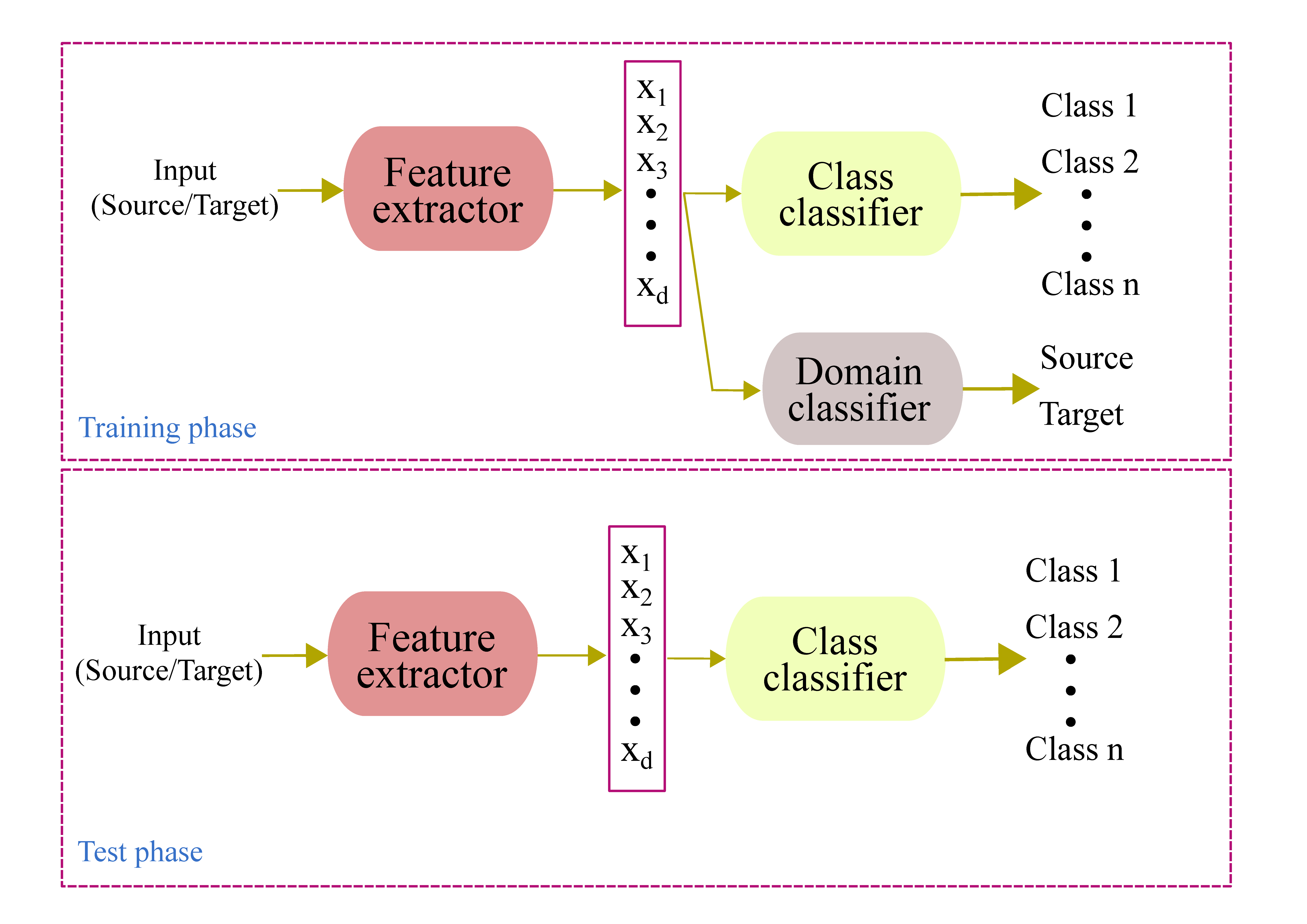
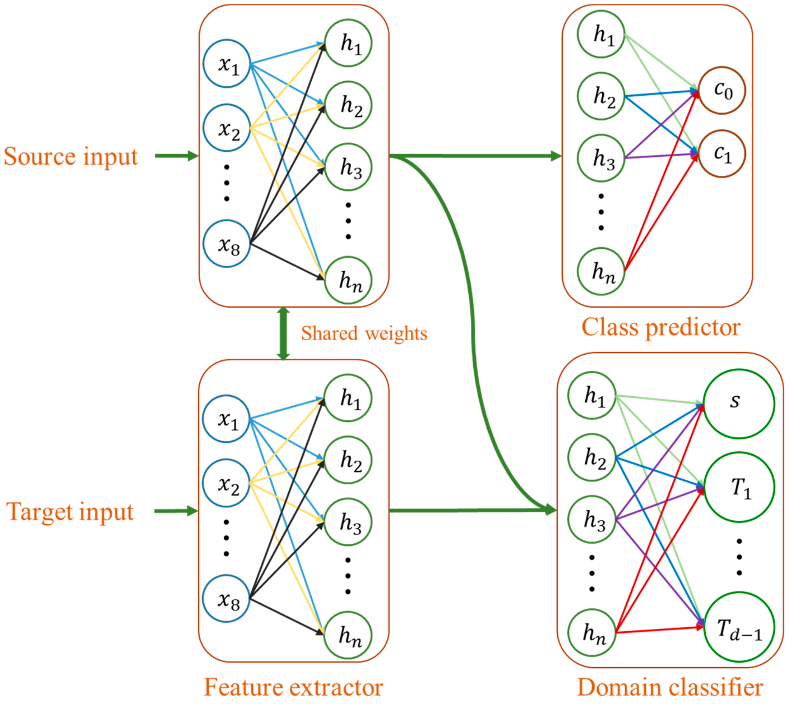
Domain adversarial neural network (DANN) is a representation learning (RL) technique in which both domain invariance and discriminative properties are taken into account while learning the mapping function, . The architecture of a DANN (Figure 1) is composed of three blocks: Feature extractor, class predictor, and domain classifier. The feature extractor is a standard feed-forward network that learns a mapping function, which transforms the input to a new d—dimensional representation. The function, F, has learnable parameters, . Similarly, both the class predictor and domain classifier are feed-forward networks that learn mapping functions, and , where and are the number of classes and domains, respectively. Both the class predictor and domain predictors have learnable parameters and , respectively. The objective of the class predictor is to learn mapping from the input space to the space of the class labels, while the objective of the domain classifier is to learn mapping from the input space to the space of the domains, that is, it predicts whether an input is sampled from the source or target domains. During training, weights of the classifier are updated to minimize classification error and weights of the domain predictor are updated to minimize domain classification error. On the other hand, the aim of the feature encoder is twofold: The first is to minimize the class prediction error and the second is to update its parameters in such a way that the domain invariance between the source and target domains is minimized. In order to accomplish this, the feature encoder maximizes the domain classifier loss, that is, when the domain classifier tries to minimize the domain classification loss, thereby increasing its ability to discriminate the source of input, the feature encoder does the opposite in order to confuse the domain classifier. Hence, the feature encoder and domain classifier work in an adversarial manner, hence the name adversarial.
Mathematically, the cost function for a DANN is expressed as
where and are the total loss for the class and domain predictors, respectively. The parameters , , and are trainable weights associated with the feature extractor, class predictor, and domain classifier, respectively. The parameter in Equation (1) is a hyper-parameter that controls the contribution of the domain discriminator to the total loss. The learning algorithm [44] updates to maximize the loss, , (Equation (3)) while keeping and fixed. Similarly, and are simultaneously updated to minimize (Equation (2)) while keeping fixed.
The gradient update rule is as follows:
In order to utilize the standard backpropagation algorithm for training, the authors in [44] proposed a gradient reversal layer (GRL) that acts as an identity transformation during forward propagation and changes the sign of a subsequent level gradient during backpropagation, that is, a gradient is multiplied by −1 before passing it to the preceding layer. The GRL is inserted between the feature extractor and domain classifier blocks and does not have parameters to be learned. Mathematically, this layer, , is defined by two equations for the forward (Equation (7)) and backpropagation (Equation (8)) properties [44]:
where is an identity matrix.
This work deals with the problem of domain adaption for large-scale land cover classification, that is, we consider remote sensing images that cover wide geographical areas acquired at different times. Such images are affected by spectral shift due to photographic distortion, changes in scale and illumination, and variation in the observed content [9], which makes it difficult to find a generic model for efficient classification. Hence, we adopt the DANN method in order to obtain a model that performs better, irrespective of the spectral shift in such images. This method takes data sampled from both source and target domains as input and learns a new representation. We also evaluate the suitability of the method to learn a generic representation for target domain samples drawn from multiple domains, referred to as multi-target domain adaptation from here on.
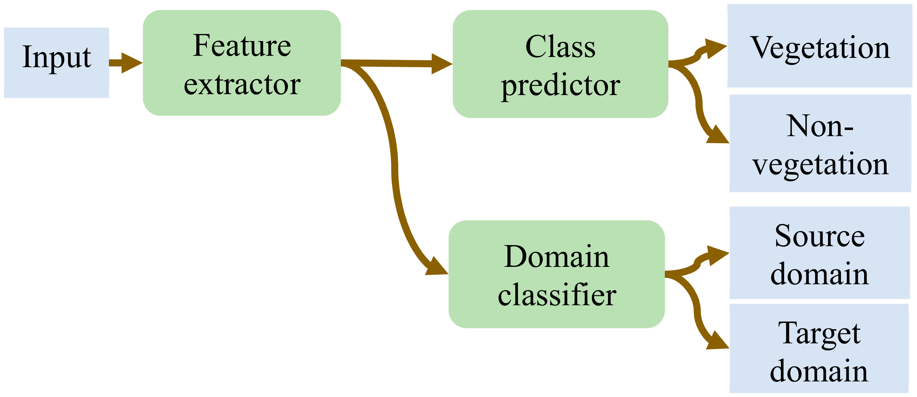
With regard to the cost function, the binary cross-entropy loss function (Equation (9)) is used for the classifier of the DANN as we are dealing with a binary classification (vegetation and non-vegetation) problem. For the domain classifier, depending on the number of target domains and the source domain, we utilize either the binary cross entropy (Equation (9)) loss or the multi-class cross entropy (Equation (10)) loss. For instance, when we are dealing with a single-target domain () the objective of the domain classifier is to distinguish whether the input data is from the source domain () or . Since we are dealing with two classes, we employ the binary cross entropy as a loss function. On the other hand, when we are seeking a domain invariant representation in the presence of a source domain () and multiple target domains (), we are dealing with a d-class classification problem and hence, we employ the multi-class cross entropy loss function.
where is the number of training samples, is the number of domains (source plus target) considered for adaptation, and and represent the true and predicted classes/domains of an input sample, respectively.
3. Experimental Results
3.1. Dataset Description
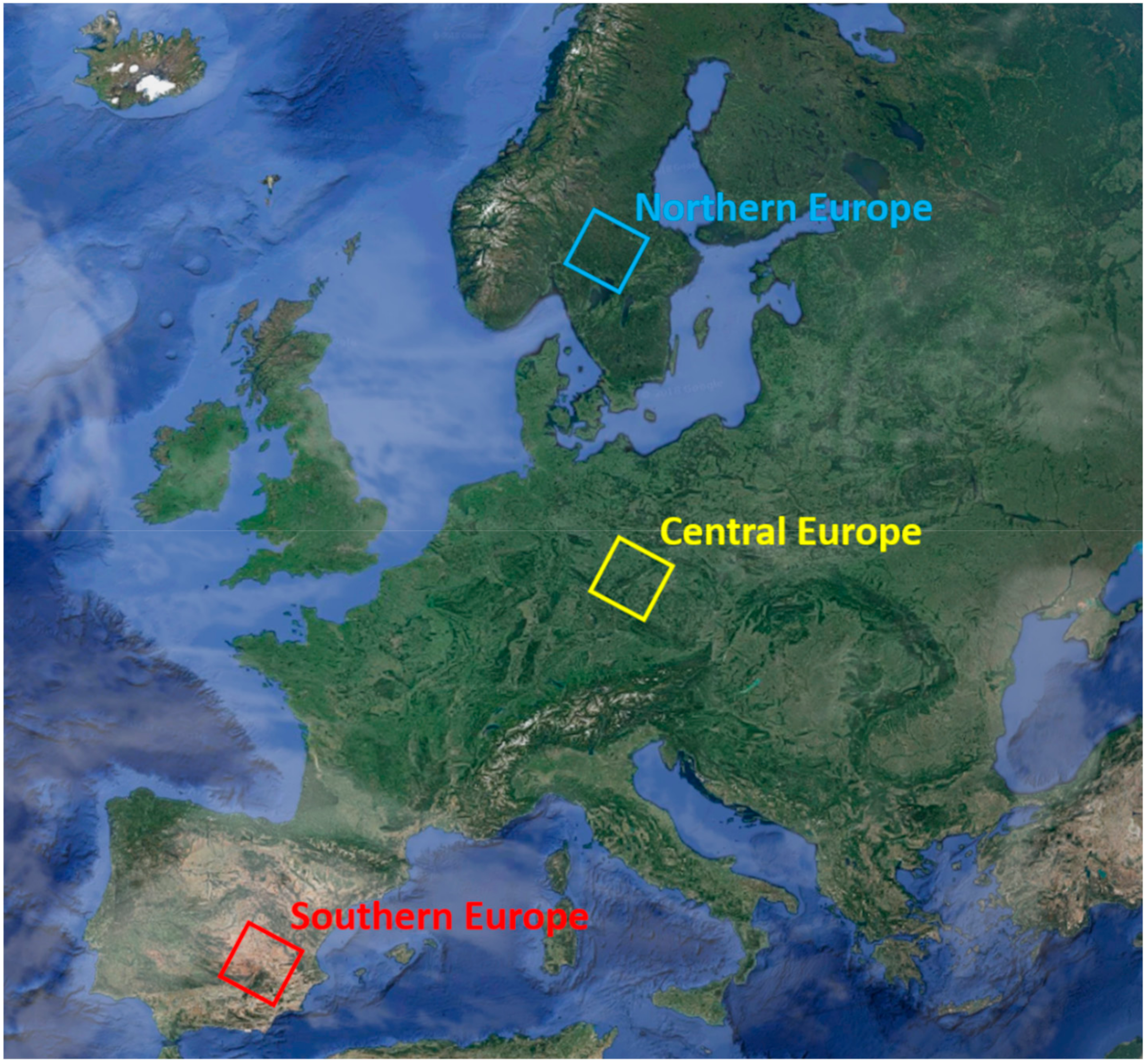
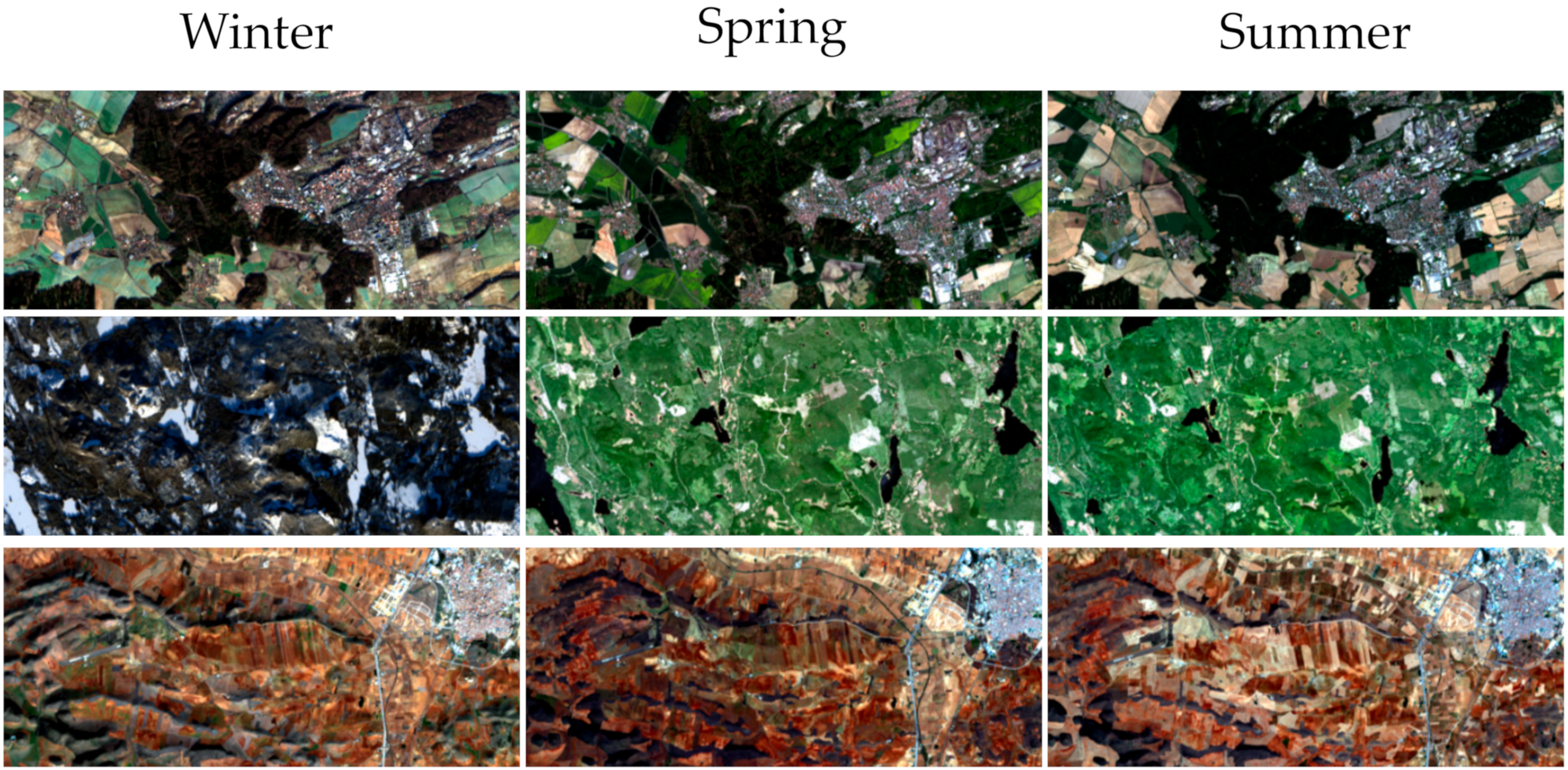
In order to validate the proposed method, we used Landsat 8 multi-spectral images characterized by a spatial resolution of 30 meters. The images were selected from three different geographical areas (Figure 2), northern, central, and southern Europe, and over three seasons, winter, spring, and summer. The winter images were acquired in January 2016, whereas the spring and summer images were acquired in May and August 2016, respectively. Moreover, each image covered a geographical area of approximately 33,000 km2 and was composed of more than 30 million pixels. Examples of images from each region per season are shown in Figure 3. For the purpose of training, we labeled parts of the images into two categories, vegetation and non-vegetation. We split the datasets into training (8000 labeled samples), validation (1000 labeled samples), and test sets. The number of labeled samples for each region per season is given in Table 1.
3.2. Experimental Setup
With regard to the network architecture (Figure 4), all three blocks were made up of fully connected layers. The output of the feature encoder was directly connected to the class classifier and the domain discriminator. The input to the feature encoder was 8-dimensional pixel samples. The main hyper-parameters of the network were the number of hidden layers, the number of neurons in each layer, the learning rate, the mini-batch training size, and lambda. In order to select the best configuration, we conducted a grid-based hyper-parameter search by training a classifier for each domain and selecting a configuration with the smallest classification loss on the corresponding domain validation set. With regard to the number of neurons in a hidden layer and the mini-batch size, we experimented with values ranging from 22 to 26 and 25 to 29, respectively. For the learning rate, the search was conducted on values ranging from 10−1 to 10−5 with a step of 0.1. Moreover, during the DANN training, the selected base learning was decreased by 0.1 every 100 training epochs. While conducting the configuration search, we observed that the accuracy on the validation sets exceeded 98% for all domains, hence we decided to limit the number of hidden layers to one. Finally, instead of using a fixed value, lambda was exponentially incremented at every epoch starting from 0 to 1. Accordingly, the best configuration for each domain is shown in Table 2. The network, implemented in Tensorflow, was kept the same for both single- and multi-target domain adaptation problems. Adam optimizer [46] was used for training with the number of training epochs fixed to 500.
3.3. Experimental Results
As mentioned in Section 2, we conducted experiments when we had single-target domain data and data from multiple target domains. As a performance metric, we report overall accuracy values (the number of correctly classified test samples divided by the total number of test samples) and provide lower bound (overall accuracy of a classifier trained on source domain data and tested with target domain data) and upper bound (overall accuracy of a classifier trained and tested with labeled samples from the target domain) values for the purpose of comparison. Moreover, the reported performance values are averaged over ten experiments and the corresponding standard deviation is also reported.
3.3.1. Single-Target Domain Adaptation
In this scenario, we conducted experiments where one of the domains, for example, northeast summer (NESU), was considered as a source domain data and the others, such as southeast winter (SEWI), were individually considered as target domain samples. We categorized these experiments into three main groups. The first and second group of experiments attempted to perform spatial (the distribution shift between source and target domains was due to the geographical difference between the samples) and temporal (the distribution shift between source and target domains was due to the difference in acquisition time) domain adaptations, respectively, whereas the third group of experiments dealt with spatiotemporal domain adaptation. The distribution shift was due to both geographical and temporal, which was more challenging compared to the first two scenarios.
In the case of spatial domain adaptation (Table 3, Table 4 and Table 5), the proposed method provided an improvement ranging from 1.1% to 14.1% in the overall accuracy of target domain samples compared to the lower boundary values in most of the source-target domain combinations. However, there were exceptions where the performance of the proposed method was much lower than the corresponding lower boundary. For instance, when northeast winter (NEWI) was used as a source domain, the performance on target domains central-east winter (CEWI) and SEWI dropped by 9.7% and 11.9%, respectively. Similarly, for the southeast summer (SESU)–NESU and SESU–central-east summer (CESU) experiments, the accuracy dropped by 19.1% and 11.6%, respectively. However, DANN performance improved when the source and target domains were interchanged. A possible reason for the decrease (increase in the reverse direction) in performance could be due to the difference in the network hyper-parameters employed for training.
Similar to the spatial domain adaptation, the proposed method yielded an increment of the overall accuracy ranging from 0.6% to more than 32%, with respect to the corresponding lower boundary accuracy values for more than half the temporal source-target pair experiments (Table 6, Table 7 and Table 8). Similar to the spatial DA case, there were source-target pairs where the proposed method had lower performance compared to the lower boundary. The most significant decreases in performance were observed for the NEWI–northeast spring (NESP), NEWI–NESU, and CESU–CEWI experiments where the accuracies dropped by 21.5%, 40.7%, and 27.9%, respectively. Considering the reverse direction (target-source), there was a decrease in performance, with the exception of CESU–CEWI, where the accuracy increased by 6.8%. However, the decreases were very small. Besides the network configuration difference in the sour-target and target-source pairs, a possible reason for the decline in performance is that the considered source domain can have a positive or negative impact on the DA process.
In the third category of experiments, we evaluated the suitability of the proposed method for spatiotemporal domain adaptation problems. In such cases, the distribution shift between source and target domains is a combined result of both temporal and spatial shift, which makes it challenging compared to the first two categories. From the results in Table 9, Table 10 and Table 11, the proposed method outperformed the lower boundary accuracy values in most of the source-target domain combinations, with an increase in the overall accuracy ranging from 0.2% to 37.1%. The challenging nature of the spatiotemporal DA was also observed from the results provided in Table 9, Table 10 and Table 11. Among the thirty-six source-target pair experiments, the proposed method failed to improve the overall accuracy compared to the lower boundary in fifteen of the experiments. Among those pairs, the largest decrease in performance was observed in the SESU–NESP (27.7% decrease) and NEWI–central-east spring (CESP) (17.2% decrease) experiments. On the other hand, if we consider the reverse directions, specifically the NESP–SESU and CESP–NEWI experiments, DANN improved the overall accuracy by 2.8% and −6.1%, respectively. Similar to the spatial and temporal experiments, the decline in performance observed in the spatiotemporal experiments was possibly due to the architecture difference and the choice of the source domain considered for the process.
3.3.2. Multi-Target Domain Adaptation
The objective of multi-target domain adaptation was to have a single model that performed well on two or more target domain datasets that had temporal, spatial, and/or spatiotemporal distribution shift. Accordingly, we modified the domain discriminator to a multi-class classifier that utilized the multi-class cross entropy loss (Equation (10)) as a cost function. In order to understand the performance of the proposed method for multi-domain adaptation, we chose two source domains (CE Spring (CESP) and NE Winter (NEWI)) based on their performance on the single-domain adaptation problem, that is, we selected the best and worst source domains based on the average increment of the target domain samples. In addition, since there were a lot of possible combinations, we limited the analysis by ranking the performance improvement in descending order and incremented the number of domains. We report the overall accuracy along with the upper and lower bound values obtained for target domains ranging from two to eight. Similar to the single-domain case, the reported results are averaged over ten experiments.
From the results in Table 12, Table 13, Table 14, Table 15, Table 16, Table 17 and Table 18, the proposed method provided an improvement in the overall accuracy ranging from 1% to 34.9% with respect to the lower boundary accuracy in almost all of the experiments in the case of the CESP source domain. Comparing the multi-domain performances with respect to the single-domain, as the number of the target domains increased from two to seven, the maximum decrease in accuracy was not more than 7%. When there were eight target domains, the accuracy for CESP–NEWI decreased by 15.8% compared to the corresponding single-domain result. On the other hand, the performance results in Table 12, Table 13, Table 14, Table 15, Table 16, Table 17 and Table 18 show that using the NEWI as a source domain for multi-target domain adaptation does not provide improvement in almost all of the source-target combination experiments. The maximum increment obtained with this setup was not more than 4%, regardless of the number of target domains. This is mainly due to the distribution of the NEWI dataset, which is discussed in Section 4.
3.4. Comparison
Besides the lower bound performance values, we compared the proposed method with denoising auto-encoders (DAEs) [47]. A DAE is a type of auto-encoder that aims to learn a mapping function that can reconstruct a “clean” input from its corrupted version by first encoding the input into a new latent space and then decoding back the input from the latent space. Following the same setup as in [16], we conducted feature encoding using this method in two settings: The first setup used only source domain samples, i.e., , to learn the encoding and the second setting used both source and target domain training samples, i.e., , to learn the encoding. We termed these settings as 1-DOM and 2-DOM, respectively. After the encoding, we trained a softmax classifier using the encoded source domain samples and classified target domain samples. The DAE parameters, such as the number of hidden layers, the number of neurons in a hidden layer, the learning rate, and the mini-batch training size, followed the same configuration used for the DANN (Table 2). During the training of the DAE, a noise sampled from a normal distribution with a mean of and a standard deviation of was added to the input.
For the purpose of comparison, we focus on single-target DA problems and report the results obtained on the best and worst source-target experiments from the spatial, temporal, and spatiotemporal DA problems. From the results in Table 19, except for the NEWI–NESU experiment, the proposed method significantly outperformed DAEs.
4. Discussion
From the experimental results reported in Section 3, the proposed method provides significant improvement in performance when compared to the accuracy values of the lower boundary and the two-stage DA approaches considered. However, there are scenarios where the method fails to improve performance. Our observations are as follows: The performance decline in the multi-target domain adaptation scenarios with the increase in the number of domains is an indication that learning a domain-invariant representation in the presence of multiple targets is more challenging compared to the single-domain adaptation. In addition, the new mapping can have positive impact on performance of some domains and negative impact on other domains. For instance, the overall accuracy for the target domain SEWI increased by more than 2% while the accuracy for the NESU target domain dropped by more than in the three-target domain experiment compared to the corresponding single-domain result. Another observation related to both the single-domain and multi-domain adaptation results is that the source domain has an impact on the domain adaptation results. That is, there are combinations (such as SEWI–SESU and SEWI–NESP) where the source-target mapping performs very well and the reverse direction (when the target is used as a source and the source is used as a target) does not work. This shows that the DA process is impacted by the choice of the source domain.
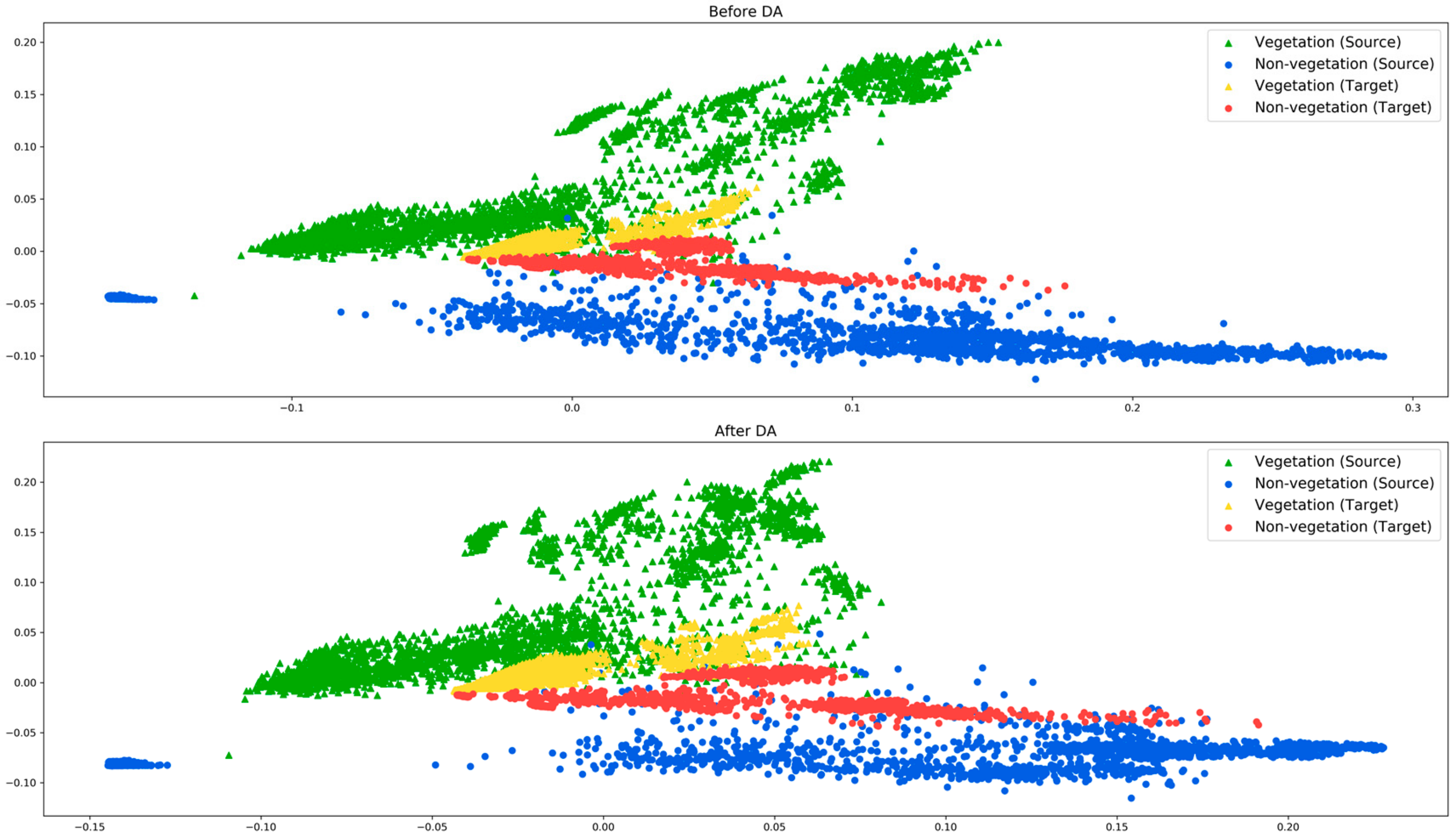
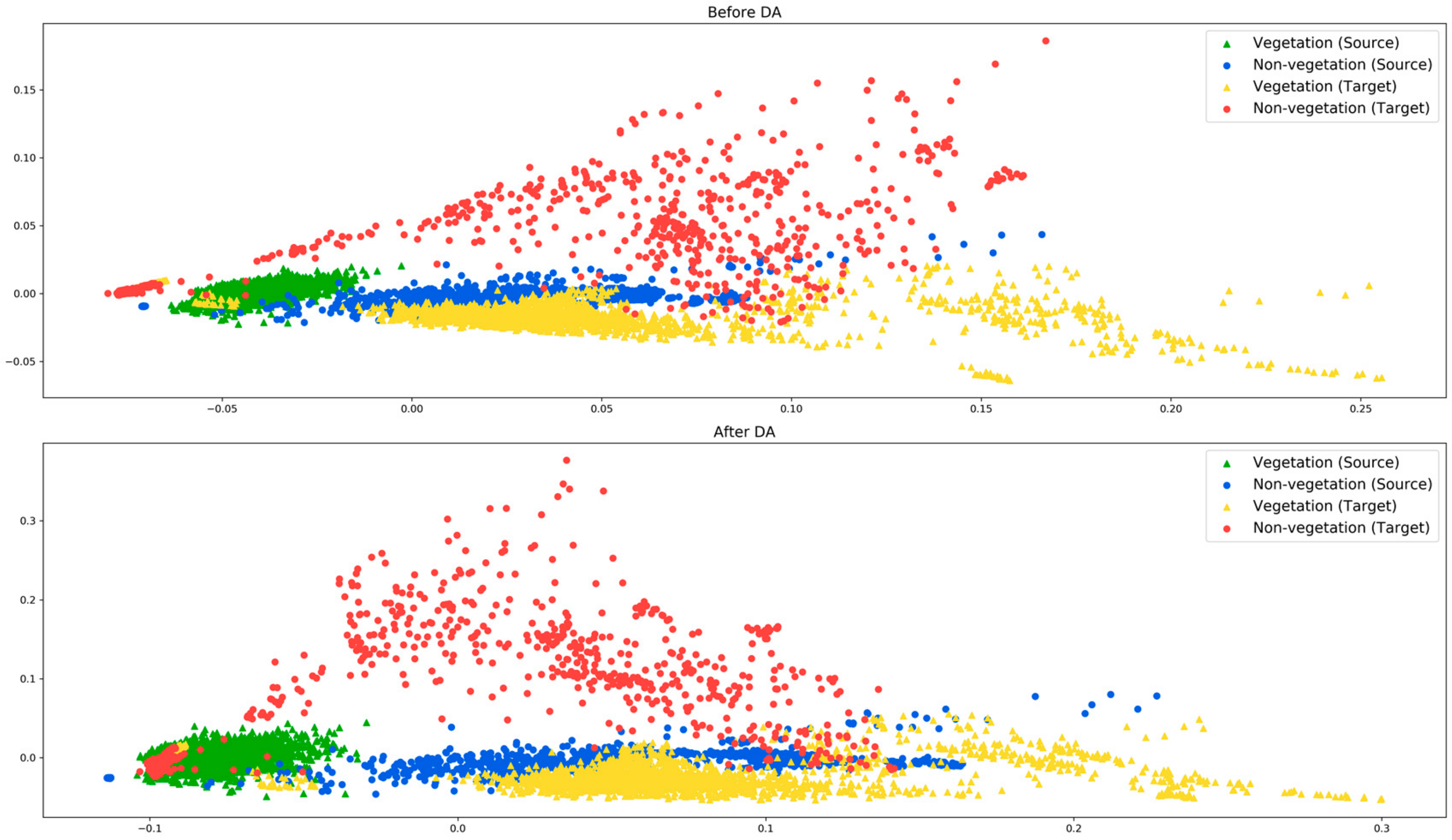
Our main observation is that the efficacy of the proposed method relies on how well the source and target domains are aligned. To explain this, we use two source-target pair experiments, the CESP–CEWI and the NEWI–NESU. The principal component analysis (PCA) distributions of the corresponding pairs before and after the domain adaptation are shown in Figure 5 and Figure 6. In Figure 5, both vegetation and non-vegetation samples from the source and target domains are roughly aligned in the same direction. Therefore, during the DA process, the vegetation and non-vegetation samples from both domains are grouped together. On the other hand, in Figure 6, the target domain vegetation samples overlap with the non-vegetation samples of the source domain. This is a possible indicator that the source and target distributions have a significant difference. This is also justified from the experimental results obtained in both single- and multi-target domain setups, where there is a significant drop in performance in almost all combinations when the NEWI domain is involved in the DA process.
5. Conclusions
Supervised classification problems require sufficiently labeled data for training, however, obtaining labeled data is not always feasible as it is a manual process that requires time and money. Unsupervised domain adaptation is an alternative approach proposed to mitigate the requirement of labeled data. This approach utilizes existing labeled data (also called the source domain) that is related to the data at hand (also called the target domain) to train a model. The objective of such methods is to minimize the distribution shift due to temporal, spatial, and/or spatiotemporal difference between the two domains and eventually to use a model trained on source domain samples to classify target domain samples. In this paper, we presented a domain adaptation technique called domain adversarial neural networks (DANNs) based on neural networks in the context of large-scale land cover classification.
In contrary to other unsupervised domain adaptation methods that consider a two-stage approach to reduce the distribution shift and then learn a classification model, DANN performs the domain adaptation and classifier learning in a single stage, thereby learning features that are both discriminative and domain invariant. Compared to the standard neural network based classifiers, DANNs have an additional block that functions as a domain classifier and provides an additional loss that correlates with the domain discrepancy. In this work, we evaluated the usefulness of DANNs both in single- and multi-target domain adaptation scenarios. In both scenarios, the proposed method provides significant improvement, with the exception of some experiments, in the overall accuracy compared to the lower boundary. The exceptions indicate that the adaptation process is asymmetric, that is, if a specific source-target pair provides improvement, the reverse (target-source) pair may not improve the accuracy. This indicates that the source domain has an impact on the adaptation process. In addition, multi-target domain adaptation experiments also show that, with the increase in the number of target domains, the suitability of the new mapping to all target domains decreases. Finally, in future work we will consider the incorporation of a mechanism that can possibly indicate whether the risk of accuracy drop is high or not based on the source and target domains considered for the process of adaptation.
Author Contributions
Conceptualization: M.B.B., F.M.; data curation: P.B.; formal analysis: M.B.B., F.M.; investigation: P.B.; Methodology: M.B.B., P.B.; project administration: F.M.; software: P.B., M.B.B.; supervision: F.M.; validation: P.B.; visualization: M.B.B.; writing-original draft: M.B.B.; writing-review and editing: F.M.
Funding
This research received no external funding.
Acknowledgments
We would like to thank the U.S Geological Survey for providing Landsat 8 images used in this work.
Conflicts of Interest
The authors declare no conflict of interest.
References
- Moranduzzo, T.; Melgani, F. Automatic Car Counting Method for Unmanned Aerial Vehicle Images. IEEE Trans. Geosci. Remote Sens. 2014, 52, 1635–1647. [Google Scholar] [CrossRef]
- Moranduzzo, T.; Melgani, F. Detecting Cars in UAV Images with a Catalog-Based Approach. IEEE Trans. Geosci. Remote Sens. 2014, 52, 6356–6367. [Google Scholar] [CrossRef]
- Cortes, C.; Vapnik, V. Support-vector networks. Mach. Learn. 1995, 20, 273–297. [Google Scholar] [CrossRef]
- Deng, J.; Dong, W.; Socher, R.; Li, L. ImageNet: A large-scale hierarchical image database. In Proceedings of the 2009 IEEE Conference on Computer Vision and Pattern Recognition, Miami, FL, USA, 20–25 June 2009; pp. 248–255. [Google Scholar]
- Bejiga, M.B.; Zeggada, A.; Nouffidj, A.; Melgani, F. A Convolutional Neural Network Approach for Assisting Avalanche Search and Rescue Operations with UAV Imagery. Remote Sens. 2017, 9, 100. [Google Scholar] [CrossRef]
- Cheng, G.; Li, Z.; Han, J.; Yao, X.; Guo, L. Exploring Hierarchical Convolutional Features for Hyperspectral Image Classification. IEEE Trans. Geosci. Remote Sens. 2018, 56, 6712–6722. [Google Scholar] [CrossRef]
- Zhou, P.; Han, J.; Cheng, G.; Zhang, B. Learning Compact and Discriminative Stacked Autoencoder for Hyperspectral Image Classification. IEEE Trans. Geosci. Remote Sens. 2019. [Google Scholar] [CrossRef]
- Cheng, G.; Yang, C.; Yao, X.; Guo, L.; Han, J. When Deep Learning Meets Metric Learning: Remote Sensing Image Scene Classification via Learning Discriminative CNNs. IEEE Trans. Geosci. Remote Sens. 2018, 56, 2811–2821. [Google Scholar] [CrossRef]
- Tuia, D.; Persello, C.; Bruzzone, L. Domain Adaptation for the Classification of Remote Sensing Data: An Overview of Recent Advances. IEEE Geosci. Remote Sens. Mag. 2016, 4, 41–57. [Google Scholar] [CrossRef]
- Verrelst, J.; Alonso, L.; Caicedo, J.P.R.; Moreno, J.; Camps-Valls, G. Gaussian Process Retrieval of Chlorophyll Content from Imaging Spectroscopy Data. IEEE J. Sel. Top. Appl. Earth Observ. Remote Sens. 2013, 6, 867–874. [Google Scholar] [CrossRef]
- Ballanti, L.; Blesius, L.; Hines, E.; Kruse, B. Tree Species Classification Using Hyperspectral Imagery: A Comparison of Two Classifiers. Remote Sens. 2016, 8, 445. [Google Scholar] [CrossRef]
- Persello, C.; Bruzzone, L. A novel approach to the selection of spatially invariant features for classification of hyperspectral images. In Proceedings of the 2009 IEEE International Geoscience and Remote Sensing Symposium, Cape Town, South Africa, 12–17 July 2009; Volume 2, pp. II-61–II–64. [Google Scholar]
- Persello, C.; Bruzzone, L. Kernel-Based Domain-Invariant Feature Selection in Hyperspectral Images for Transfer Learning. IEEE Trans. Geosci. Remote Sens. 2016, 54, 2615–2626. [Google Scholar] [CrossRef]
- Izquierdo-Verdiguier, E.; Laparra, V.; Gómez-Chova, L.; Camps-Valls, G. Including invariances in SVM remote sensing image classification. In Proceedings of the 2012 IEEE International Geoscience and Remote Sensing Symposium, Munich, Germany, 22–27 July 2012; pp. 7353–7356. [Google Scholar]
- Inamdar, S.; Bovolo, F.; Bruzzone, L.; Chaudhuri, S. Multidimensional Probability Density Function Matching for Preprocessing of Multitemporal Remote Sensing Images. IEEE Trans. Geosci. Remote Sens. 2008, 46, 1243–1252. [Google Scholar] [CrossRef]
- Matasci, G.; Volpi, M.; Kanevski, M.; Bruzzone, L.; Tuia, D. Semisupervised Transfer Component Analysis for Domain Adaptation in Remote Sensing Image Classification. IEEE Trans. Geosci. Remote Sens. 2015, 53, 3550–3564. [Google Scholar] [CrossRef]
- Pan, S.J.; Tsang, I.W.; Kwok, J.T.; Yang, Q. Domain Adaptation via Transfer Component Analysis. IEEE Trans. Neural Netw. 2011, 22, 199–210. [Google Scholar] [CrossRef]
- Volpi, M.; Camps-Valls, G.; Tuia, D. Spectral alignment of multi-temporal cross-sensor images with automated kernel canonical correlation analysis. ISPRS J. Photogramm. Remote Sens. 2015, 107, 50–63. [Google Scholar] [CrossRef]
- Jun, G.; Ghosh, J. Spatially Adaptive Classification of Land Cover with Remote Sensing Data. IEEE Trans. Geosci. Remote Sens. 2011, 49, 2662–2673. [Google Scholar] [CrossRef]
- Gonzalez, D.M.; Camps-Valls, G.; Tuia, D. Weakly supervised alignment of multisensor images. In Proceedings of the 2015 IEEE International Geoscience and Remote Sensing Symposium (IGARSS), Milan, Italy, 26–31 July 2015; pp. 2588–2591. [Google Scholar]
- Tuia, D.; Volpi, M.; Trolliet, M.; Camps-Valls, G. Semisupervised Manifold Alignment of Multimodal Remote Sensing Images. IEEE Trans. Geosci. Remote Sens. 2014, 52, 7708–7720. [Google Scholar] [CrossRef]
- Yang, H.L.; Crawford, M.M. Spectral and Spatial Proximity-Based Manifold Alignment for Multitemporal Hyperspectral Image Classification. IEEE Trans. Geosci. Remote Sens. 2016, 54, 51–64. [Google Scholar] [CrossRef]
- Yang, H.L.; Crawford, M.M. Domain Adaptation with Preservation of Manifold Geometry for Hyperspectral Image Classification. IEEE J. Sel. Top. Appl. Earth Observ. Remote Sens. 2016, 9, 543–555. [Google Scholar] [CrossRef]
- Tuia, D.; Munoz-Mari, J.; Gomez-Chova, L.; Malo, J. Graph Matching for Adaptation in Remote Sensing. IEEE Trans. Geosci. Remote Sens. 2013, 51, 329–341. [Google Scholar] [CrossRef]
- Othman, E.; Bazi, Y.; Alajlan, N.; AlHichri, H.; Melgani, F. Three-Layer Convex Network for Domain Adaptation in Multitemporal VHR Images. IEEE Geosci. Remote Sens. Lett. 2016, 13, 354–358. [Google Scholar] [CrossRef]
- Bencherif, M.A.; Bazi, Y.; Guessoum, A.; Alajlan, N.; Melgani, F.; AlHichri, H. Fusion of Extreme Learning Machine and Graph-Based Optimization Methods for Active Classification of Remote Sensing Images. IEEE Geosci. Remote Sens. Lett. 2015, 12, 527–531. [Google Scholar] [CrossRef]
- Sun, H.; Liu, S.; Zhou, S.; Zou, H. Transfer Sparse Subspace Analysis for Unsupervised Cross-View Scene Model Adaptation. IEEE J. Sel. Top. Appl. Earth Observ. Remote Sens. 2016, 9, 2901–2909. [Google Scholar] [CrossRef]
- Rajan, S.; Ghosh, J.; Crawford, M.M. Exploiting Class Hierarchies for Knowledge Transfer in Hyperspectral Data. IEEE Trans. Geosci. Remote Sens. 2006, 44, 3408–3417. [Google Scholar] [CrossRef]
- Bruzzone, L.; Marconcini, M. Domain Adaptation Problems: A DASVM Classification Technique and a Circular Validation Strategy. IEEE Trans. Pattern Anal. Mach. Intell. 2010, 32, 770–787. [Google Scholar] [CrossRef] [PubMed]
- Sun, Z.; Wang, C.; Wang, H.; Li, J. Learn Multiple-Kernel SVMs for Domain Adaptation in Hyperspectral Data. IEEE Geosci. Remote Sens. Lett. 2013, 10, 1224–1228. [Google Scholar]
- Gomez-Chova, L.; Camps-Valls, G.; Munoz-Mari, J.; Calpe, J. Semisupervised Image Classification with Laplacian Support Vector Machines. IEEE Geosci. Remote Sens. Lett. 2008, 5, 336–340. [Google Scholar] [CrossRef]
- Chi, M.; Bruzzone, L. Semisupervised Classification of Hyperspectral Images by SVMs Optimized in the Primal. IEEE Trans. Geosci. Remote Sens. 2007, 45, 1870–1880. [Google Scholar] [CrossRef]
- Bruzzone, L.; Chi, M.; Marconcini, M. A Novel Transductive SVM for Semisupervised Classification of Remote-Sensing Images. IEEE Trans. Geosci. Remote Sens. 2006, 44, 3363–3373. [Google Scholar] [CrossRef]
- Leiva-Murillo, J.M.; Gomez-Chova, L.; Camps-Valls, G. Multitask Remote Sensing Data Classification. IEEE Trans. Geosci. Remote Sens. 2013, 51, 151–161. [Google Scholar] [CrossRef]
- Rajan, S.; Ghosh, J.; Crawford, M.M. An Active Learning Approach to Hyperspectral Data Classification. IEEE Trans. Geosci. Remote Sens. 2008, 46, 1231–1242. [Google Scholar] [CrossRef]
- Tuia, D.; Ratle, F.; Pacifici, F.; Kanevski, M.F.; Emery, W.J. Active Learning Methods for Remote Sensing Image Classification. IEEE Trans. Geosci. Remote Sens. 2009, 47, 2218–2232. [Google Scholar] [CrossRef]
- Tuia, D.; Pasolli, E.; Emery, W.J. Using active learning to adapt remote sensing image classifiers. Remote Sens. Environ. 2011, 115, 2232–2242. [Google Scholar] [CrossRef]
- Matasci, G.; Tuia, D.; Kanevski, M. SVM-Based Boosting of Active Learning Strategies for Efficient Domain Adaptation. IEEE J. Sel. Top. Appl. Earth Observ. Remote Sens. 2012, 5, 1335–1343. [Google Scholar] [CrossRef]
- Persello, C.; Bruzzone, L. Active Learning for Domain Adaptation in the Supervised Classification of Remote Sensing Images. IEEE Trans. Geosci. Remote Sens. 2012, 50, 4468–4483. [Google Scholar] [CrossRef]
- Alajlan, N.; Pasolli, E.; Melgani, F.; Franzoso, A. Large-Scale Image Classification Using Active Learning. IEEE Geosci. Remote Sens. Lett. 2014, 11, 259–263. [Google Scholar] [CrossRef]
- Persello, C.; Boularias, A.; Dalponte, M.; Gobakken, T.; Næsset, E.; Schölkopf, B. Cost-Sensitive Active Learning with Lookahead: Optimizing Field Surveys for Remote Sensing Data Classification. IEEE Trans. Geosci. Remote Sens. 2014, 52, 6652–6664. [Google Scholar] [CrossRef]
- Demir, B.; Minello, L.; Bruzzone, L. Definition of Effective Training Sets for Supervised Classification of Remote Sensing Images by a Novel Cost-Sensitive Active Learning Method. IEEE Trans. Geosci. Remote Sens. 2014, 52, 1272–1284. [Google Scholar] [CrossRef]
- Stumpf, A.; Lachiche, N.; Malet, J.P.; Kerle, N.; Puissant, A. Active Learning in the Spatial Domain for Remote Sensing Image Classification. IEEE Trans. Geosci. Remote Sens. 2014, 52, 2492–2507. [Google Scholar] [CrossRef]
- Ganin, Y.; Ustinova, E.; Ajakan, H.; Germain, P.; Larochelle, H.; Laviolette, F.; Marchand, M.; Lempitsky, V. Domain-Adversarial Training of Neural Networks. In Domain Adaptation in Computer Vision Applications; Csurka, G., Ed.; Springer International Publishing: Cham, Switzerland, 2017; pp. 189–209. ISBN 978-3-319-58346-4. [Google Scholar]
- Elshamli, A.; Taylor, G.W.; Berg, A.; Areibi, S. Domain Adaptation Using Representation Learning for the Classification of Remote Sensing Images. IEEE J. Sel. Top. Appl. Earth Observ. Remote Sens. 2017, 10, 4198–4209. [Google Scholar] [CrossRef]
- Kingma, D.P.; Ba, J. Adam: A Method for Stochastic Optimization. arXiv 2014, arXiv:1412.6980. [Google Scholar]
- Vincent, P.; Larochelle, H.; Bengio, Y.; Manzagol, P.-A. Extracting and composing robust features with denoising autoencoders. In Proceedings of the 25th International Conference on Machine Learning, Helsinki, Finland, 5–9 July 2008; pp. 1096–1103. [Google Scholar]
Figure 1.
Block diagram of a domain adversarial neural network’s (DANN’s) architecture. The output of the feature extractor is a representation of an input in the new latent space, which is then directly fed to the class and domain classifiers.
Figure 1.
Block diagram of a domain adversarial neural network’s (DANN’s) architecture. The output of the feature extractor is a representation of an input in the new latent space, which is then directly fed to the class and domain classifiers.

Figure 2.
The three geographical areas considered for the study.

Figure 3.
Sample image crops from the central-east (top), northeast (middle), and southeast (bottom) regions.
Figure 3.
Sample image crops from the central-east (top), northeast (middle), and southeast (bottom) regions.

Figure 4.
Network architecture based on fully connected layers employed for training.

Figure 5.
PCA distribution of source (CESP) and target domain (CEWI) test samples before (top) and after (bottom) domain adaptation.
Figure 5.
PCA distribution of source (CESP) and target domain (CEWI) test samples before (top) and after (bottom) domain adaptation.

Figure 6.
PCA distribution of source (NEWI) and target domain (NESU) test samples before (top) and after (bottom) domain adaptation.
Figure 6.
PCA distribution of source (NEWI) and target domain (NESU) test samples before (top) and after (bottom) domain adaptation.


Table 1.
Labeled pixel samples used for training and tests from both domains. Central-east (CE), northeast (NE), southeast (SE).
Table 1.
Labeled pixel samples used for training and tests from both domains. Central-east (CE), northeast (NE), southeast (SE).
| Domain | Vegetation | Non-Vegetation |
|---|---|---|
| CE Spring (CESP) | 7668 | 7405 |
| CE Summer (CESU) | 7531 | 7161 |
| CE Winter (CEWI) | 6995 | 6857 |
| NE Spring (NESP) | 6315 | 6081 |
| NE Summer (NESU) | 6529 | 6869 |
| NE Winter (NEWI) | 7210 | 7061 |
| SE Spring (SESP) | 7356 | 7380 |
| SE Summer (SESU) | 7102 | 7343 |
| SE Winter (SEWI) | 7346 | 7343 |
Table 2.
Mini-batch size, learning rate, and the number of neurons used for training depending on the source domain considered.
Table 2.
Mini-batch size, learning rate, and the number of neurons used for training depending on the source domain considered.
| Source Domain | Learning Rate | Number of Neurons | Mini-Batch Size |
|---|---|---|---|
| CESP | 10−2 | 64 | 256 |
| CESU | 10−2 | 32 | 32 |
| CEWI | 10−1 | 32 | 32 |
| NESP | 10−1 | 4 | 128 |
| NESU | 10−2 | 64 | 128 |
| NEWI | 10−2 | 16 | 512 |
| SESP | 10−2 | 32 | 32 |
| SESU | 10−2 | 32 | 256 |
| SEWI | 10−2 | 64 | 64 |
Table 3.
Spatial domain adaptation average overall accuracy (in %) and standard deviation results realized over ten independent runs for the spring season. Rows in green and blue are the results of the proposed method and lower bound values, respectively. The upper bound accuracy is shown at the top of each row in brackets. Values in bold and red fonts indicate an increase and decrease in accuracy, respectively, by the proposed method compared to the lower-bound.
| Target Domain | ||||
|---|---|---|---|---|
| Source Domain | NESP (99.9, 0.003) | CESP (1.0, 0.0) | SESP (99.5, 0.005) | |
| NESP | 99.3, 0.013 | 81.5, 0.033 | ||
| 98.1, 0.022 | 71.7, 0.051 | |||
| CESP | 96.7, 0.011 | 83.8, 0.062 | ||
| 88.7, 0.078 | 69.9, 0.065 | |||
| SESP | 61.5, 0.011 | 98.1, 0.011 | ||
| 64.3, 0.042 | 95.8, 0.068 | |||
Table 4.
Spatial domain adaptation average overall accuracy (in %) and standard deviation results realized over ten independent runs for the summer season. Rows in green and blue are the results of the proposed method and lower bound values, respectively. The upper bound accuracy is shown at the top of each row in brackets. Values in bold and red fonts indicate an increase and decrease in accuracy, respectively, by the proposed method compared to the lower-bound.
| Target Domain | ||||
|---|---|---|---|---|
| Source Domain | NESU (98.8, 0.004) | CESU (1.0, 0.0) | SESU (99.0, 0.0) | |
| NESU | 98.0, 0.017 | 61.6, 0.026 | ||
| 83.9, 0.010 | 53.4, 0.020 | |||
| CESU | 95.6, 0.005 | 72.0, 0.023 | ||
| 95.8, 0.004 | 66.9, 0.020 | |||
| SESU | 68.0, 0.173 | 83.8, 0.059 | ||
| 87.1, 0.087 | 95.4, 0.016 | |||
Table 5.
Spatial domain adaptation average overall accuracy (in %) and standard deviation results realized over ten independent runs for the winter season. Rows in green and blue are the results of the proposed method and lower bound values, respectively. The upper bound accuracy is shown at the top of each row in brackets. Values in bold and red fonts indicate an increase and decrease in accuracy, respectively, by the proposed method compared to the lower-bound.
| Target Domain | ||||
|---|---|---|---|---|
| Source Domain | NEWI (1.0, 0.0) | CEWI (99.6, 0.009) | SEWI (1.0, 0.0) | |
| NEWI | 71.7, 0.026 | 83.3, 0.093 | ||
| 81.4, 0.062 | 95.2, 0.014 | |||
| CEWI | 73.2, 0.045 | 87.6, 0.024 | ||
| 63.2, 0.042 | 88.4, 0.038 | |||
| SEWI | 89.1, 0.085 | 74.2, 0.009 | ||
| 91.1, 0.045 | 71.5, 0.022 | |||
Table 6.
Temporal domain adaptation average overall accuracy (in %) and standard deviation results realized over ten independent runs for the northeast region. Rows in green and blue are the results of the proposed method and lower bound values, respectively. The upper bound accuracy is shown at the top of each row in brackets. Values in bold and red fonts indicate an increase and decrease in accuracy, respectively, by the proposed method compared to the lower-bound.
| Target Domain | ||||
|---|---|---|---|---|
| Source Domain | NESP (99.9, 0.003) | NESU (98.8, 0.04) | NEWI (1.0, 0.0) | |
| NESP | 94.4, 0.005 | 83.9, 0.120 | ||
| 95.0, 0.004 | 86.0, 0.132 | |||
| NESU | 93.8, 0.027 | 73.7, 0.175 | ||
| 61.3, 0.028 | 82.2, 0.059 | |||
| NEWI | 73.1, 0.096 | 34.1, 0.228 | ||
| 94.5, 0.036 | 74.8, 0.130 | |||
Table 7.
Temporal domain adaptation average overall accuracy (in %) and standard deviation results realized over ten independent runs for the central-east region. Rows in green and blue are the results of the proposed method and lower bound values, respectively. The upper bound accuracy is shown at the top of each row in brackets. Values in bold and red fonts indicate an increase and decrease in accuracy by the proposed method compared to the lower-bound.
| Target Domain | ||||
|---|---|---|---|---|
| Source Domain | CESP (1.0, 0.0) | CESU (1.0, 0.0) | CEWI (99.6, 0.009) | |
| CESP | 99.0, 0.0 | 77.3, 0.125 | ||
| 98.4, 0.008 | 51.0, 0.0 | |||
| CESU | 95.3, 0.009 | 65.3, 0.078 | ||
| 94.4, 0.022 | 93.2, 0.066 | |||
| CEWI | 95.9, 0.064 | 98.6, 0.007 | ||
| 78.5, 0.102 | 91.8, 0.097 | |||
Table 8.
Temporal domain adaptation average overall accuracy (in %) and standard deviation results realized over ten independent runs for the southeast region. Rows in green and blue are the results of the proposed method and lower bound values, respectively. The upper bound accuracy is shown at the top of each row in brackets. Values in bold and red fonts indicate an increase and decrease in accuracy by the proposed method compared to the lower-bound.
| Target Domain | ||||
|---|---|---|---|---|
| Source Domain | SESP (99.5, 0.005) | SESU (99.0, 0.0) | SEWI (1.0, 0.0) | |
| SESP | 98.0, 0.0 | 87.3, 0.080 | ||
| 97.8, 0.007 | 70.3, 0.061 | |||
| SESU | 98.6, 0.005 | 69.9, 0.077 | ||
| 96.1, 0.005 | 76.8, 0.043 | |||
| SEWI | 89.8, 0.087 | 85.5, 0.088 | ||
| 61.6, 0.037 | 69.2, 0.037 | |||
Table 9.
Spatiotemporal domain adaptation average overall accuracy (in %) and standard deviation results realized over ten independent runs. Rows in green and blue are the results of the proposed method and lower bound values, respectively. The upper bound accuracy is shown at the top of each row in brackets. Values in bold and red fonts indicate an increase and decrease in accuracy by the proposed method compared to the lower-bound.
| Target Domain | |||||||
|---|---|---|---|---|---|---|---|
| Source Domain | CESP (1.0, 0.0) | CESU (1.0, 0.0) | CEWI (99.6, 0.009) | SESP (99.5, 0.005) | SESU (99.0, 0.0) | SEWI (1.0, 0.0) | |
| NESP | 99.0, 0.0 | 88.0, 0.074 | 75.5, 0.011 | 95.7, 0.015 | |||
| 98.1, 0.022 | 84.2, 0.106 | 72.7, 0.026 | 97.3, 0.013 | ||||
| NESU | 93.1, 0.029 | 86.9, 0.088 | 63.3, 0.041 | 95.5, 0.034 | |||
| 64.3, 0.067 | 62.1, 0.034 | 50.8, 0.026 | 82.9, 0.030 | ||||
| NEWI | 82.1, 0.161 | 84.6, 0.087 | 66.8, 0.156 | 65.9, 0.126 | |||
| 99.2, 0.007 | 99.0, 0.0 | 76.7, 0.073 | 72.7, 0.032 | ||||
Table 10.
Spatiotemporal domain adaptation overall accuracy (in %) results. Rows in green and blue are the results of the proposed method and lower bound values, respectively. The upper bound accuracy is shown at the top of each row in brackets. Values in bold and red fonts indicate an increase and decrease in accuracy by the proposed method compared to the lower-bound.
| Target Domain | |||||||
|---|---|---|---|---|---|---|---|
| Source Domain | NESP (99.9, 0.003) | NESU (98.8, 0.004) | NEWI (1.0, 0.0) | SESP (99.5, 0.005) | SESU (99.0, 0.0) | SEWI (1.0, 0.0) | |
| CESP | 93.9, 0.003 | 90.3, 0.128 | 81.8, 0.056 | 94.4, 0.061 | |||
| 59.7, 0.077 | 96.4, 0.005 | 89.8, 0.028 | 72.2, 0.044 | ||||
| CESU | 80.8, 0.046 | 78.3, 0.160 | 71.7, 0.047 | 84.7, 0.018 | |||
| 77.2, 0.042 | 82.9, 0.133 | 75.7, 0.024 | 86.0, 0.038 | ||||
| CEWI | 94.9, 0.051 | 95.1, 0.003 | 68.8, 0.055 | 70.4, 0.030 | |||
| 57.8, 0.054 | 93.9, 0.025 | 62.3, 0.062 | 61.7, 0.032 | ||||
Table 11.
Spatiotemporal domain adaptation average overall accuracy (in %) and standard deviation results realized over ten independent runs. Rows in green and blue are the results of the proposed method and lower bound values, respectively. The upper bound accuracy is shown at the top of each row in brackets. Values in bold and red fonts indicate an increase and decrease in accuracy by the proposed method compared to the lower-bound.
| Target Domain | |||||||
|---|---|---|---|---|---|---|---|
| Source Domain | CESP (1.0, 0.0) | CESU (1.0, 0.0) | CEWI (99.6, 0.009) | NESP (99.3, 0.003) | NESU (98.8, 0.004) | NEWI (1.0, 0.0) | |
| SESP | 81.8, 0.008 | 59.6, 0.104 | 57.7, 0.123 | 82.3, 0.117 | |||
| 91.0, 0.073 | 51.1, 0.003 | 50.8, 0.007 | 86.1, 0.062 | ||||
| SESU | 94.6, 0.067 | 67.7, 0.127 | 68.3, 0.076 | 84.5, 0.086 | |||
| 99.0, 0.0 | 62.5, 0.091 | 96.0, 0.0 | 96.7, 0.019 | ||||
| SEWI | 98.4, 0.015 | 97.9, 0.025 | 97.1, 0.008 | 95.2, 0.004 | |||
| 92.7, 0.013 | 98.7, 0.009 | 80.9, 0.024 | 95.0, 0.0 | ||||
Table 12.
Experimental results for two target domains. Average overall accuracy (in %) and standard deviation results realized over ten independent runs for the proposed method (green rows) and lower bound values (blue rows). Upper bound values are shown in the second row in brackets. Values in bold and red fonts indicate an increase and decrease in accuracy by the proposed method compared to the lower-bound.
| Target Domain | |||||
|---|---|---|---|---|---|
| Source Domain | NESU (98.8, 0.004) | SEWI (1.0, 0.0) | SESU (99.0, 0.0) | CEWI (99.6, 0.009) | |
| CESP | 89.3, 0.112 | 92.4, 0.075 | |||
| 59.7, 0.077 | 72.2, 0.44 | ||||
| NEWI | 70.3, 0.163 | 54.0, 0.034 | |||
| 72.7, 0.032 | 81.4, 0.062 | ||||
Table 13.
Experimental results for three target domains. Average overall accuracy (in %) and standard deviation results realized over ten independent runs for the proposed method (green rows) and lower bound values (blue rows). Upper bound values are shown in the second row in brackets. Values in bold and red fonts indicate an increase and decrease in accuracy by the proposed method compared to the lower-bound.
| Target Domain | ||||||
|---|---|---|---|---|---|---|
| Source Domain | NESU (98.8, 0.004) | SEWI (1.0, 0.0) | CEWI (99.6, 0.009) | SESU (99.0, 0.0) | SESP (99.5, 0.005) | |
| CESP | 90.3, 0.111 | 93.7, 0.044 | 83.7, 0.105 | |||
| 59.7, 0.077 | 72.2, 0.44 | 51.0, 0.0 | ||||
| NEWI | 53.7, 0.036 | 71.4, 0.133 | 70.4, 0.142 | |||
| 81.4, 0.062 | 72.7, 0.032 | 76.7, 0.073 | ||||
Table 14.
Experimental results for four target domains. Average overall accuracy (in %) and standard deviation results realized over ten independent runs for the proposed method (green rows) and lower bound values (blue rows). Upper bound values are shown in the second row in brackets. Values in bold and red fonts indicate an increase and decrease in accuracy by the proposed method compared to the lower-bound.
| Target Domain | ||||||
|---|---|---|---|---|---|---|
| Source Domain | NESU (98.8, 0.004) | SEWI (1.0, 0.0) | CEWI (99.6, 0.009) | SESU (99.0, 0.0) | SESP (99.5, 0.005) | |
| CESP | 88.6, 0.099 | 97.0, 0.025 | 74.9, 0.101 | 84.7, 0.028 | ||
| 59.7, 0.077 | 72.2, 0.44 | 51.0, 0.0 | 69.9, 0.065 | |||
| NEWI | 94.1, 0.065 | 70.3, 0.052 | 76.5, 0.118 | 78.6, 0.142 | ||
| 95.2, 0.014 | 81.4, 0.062 | 72.7, 0.032 | 76.7, 0.073 | |||
Table 15.
Experimental results for five target domains. Average overall accuracy (in %) and standard deviation results realized over ten independent runs for the proposed method (green rows) and lower bound values (blue rows ). Upper bound values are shown in the second row in brackets. Values in bold and red fonts indicate an increase and decrease in accuracy by the proposed method compared to the lower-bound.
| Target Domain | ||||||||
|---|---|---|---|---|---|---|---|---|
| Source Domain | NESU (98.8, 0.004) | SEWI (1.0, 0.0) | CEWI (99.6, 0.009) | SESP (99.5, 0.005) | NESP (99.9, 0.003) | SESU (99.0, 0.0) | CESU (1.0, 0.0) | |
| CESP | 93.0, 0.034 | 94.0, 0.056 | 77.9, 0.073 | 83.5, 0.035 | 95.6, 0.025 | |||
| 59.7, 0.077 | 72.2, 0.44 | 51.0, 0.0 | 69.9, 0.065 | 88.7, 0.078 | ||||
| NEWI | 94.9, 0.040 | 74.8, 0.028 | 72.3, 0.072 | 70.4, 0.048 | 98.3, 0.021 | |||
| 95.2, 0.014 | 81.4, 0.062 | 76.7, 0.073 | 72.7, 0.032 | 99.0, 0.0 | ||||
Table 16.
Experimental results for six target domains. Average overall accuracy (in %) and standard deviation results realized over ten independent runs for the proposed method (green rows) and lower bound values (blue rows). Upper bound values are shown in the second column in brackets. Values in bold and red fonts indicate an increase and decrease in accuracy by the proposed method compared to the lower-bound.
| Source Domain | |||
|---|---|---|---|
| Target Domain | CESP | NEWI | |
| CESP (1.0, 0.0) | 95.4, 0.078 | ||
| 99.2, 0.007 | |||
| NESU (98.8, 0.004) | 93.8, 0.020 | ||
| 59.7, 0.077 | |||
| SEWI (1.0, 0.0) | 93.7, 0.045 | 92.3, 0.075 | |
| 72.2, 0.440 | 95.2, 0.014 | ||
| CEWI (99.6, 0.009) | 83.5, 0.079 | 77.1, 0.032 | |
| 51.0, 0.0 | 81.4, 0.062 | ||
| SESP (99.5, 0.005) | 83.0, 0.032 | 74.5, 0.102 | |
| 69.9, 0.065 | 76.7, 0.073 | ||
| NESP (99.9, 0.003) | 95.0, 0.029 | ||
| 88.7, 0.078 | |||
| SESU (99.0, 0.0) | 71.8, 0.089 | ||
| 72.7, 0.032 | |||
| CESU (1.0, 0.0) | 99.0, 0.0 | 96.9, 0.050 | |
| 98.4, 0.008 | 99.0, 0.0 | ||
Table 17.
Experimental results for seven target domains. Average overall accuracy (in %) and standard deviation results realized over ten independent runs for the proposed method (green rows) and lower bound values (blue rows) Upper bound values are shown in the second column in brackets. Values in bold and red fonts indicate an increase and decrease in accuracy by the proposed method compared to the lower-bound.
| Source Domain | |||
|---|---|---|---|
| Target Domain | CESP | NEWI | |
| CESP (1.0, 0.0) | 99.0, 0.012 | ||
| 99.2, 0.007 | |||
| NESU (98.8, 0.004) | 94.6, 0.005 | ||
| 59.7, 0.077 | |||
| SEWI (1.0, 0.0) | 93.6, 0.045 | 94.7, 0.039 | |
| 72.2, 0.44 | 95.2, 0.014 | ||
| CEWI (99.6, 0.009) | 86.4, 0.094 | 78.5, 0.043 | |
| 81.4, 0.062 | 81.4, 0.062 | ||
| SESP (99.5, 0.005) | 82.4, 0.019 | 78.3, 0.076 | |
| 69.9, 0.065 | 76.7, 0.073 | ||
| NESP (99.9, 0.003) | 95.7, 0.035 | 94.6, 0.045 | |
| 88.7, 0.078 | 94.5, 0.036 | ||
| SESU (99.0, 0.0) | 73.6, 0.043 | ||
| 72.7, 0.032 | |||
| CESU (1.0, 0.0) | 99.0, 0.0 | 99.0, 0.0 | |
| 98.4, 0.008 | 99.0, 0.0 | ||
| NEWI (1.0, 0.0) | 72.8, 0.197 | ||
| 96.4, 0.005 | |||
Table 18.
Experimental results for eight target domains. Green rows are overall accuracy (in %) values of the proposed method and blue rows are lower bound values. Upper bound values are shown in the second column in brackets. Values in bold and red fonts indicate an increase and decrease in accuracy by the proposed method compared to the lower-bound.
| Source Domain | |||
|---|---|---|---|
| Target Domain | CESP | NEWI | |
| CESP (1.0, 0.0) | 97.0, 0.057 | ||
| 99.2, 0.007 | |||
| NESU (98.8, 0.004) | 92.5, 0.014 | 94.6, 0.008 | |
| 59.7, 0.077 | 74.8, 0.130 | ||
| SEWI (1.0, 0.0) | 91.2, 0.077 | 92.4, 0.065 | |
| 72.2, 0.440 | 95.2, 0.014 | ||
| CEWI (99.6, 0.009) | 70.6, 0.084 | 79.5, 0.055 | |
| 51.0, 0.0 | 81.4, 0.062 | ||
| SESP (99.5, 0.005) | 85.5, 0.046 | 75.5, 0.085 | |
| 69.9, 0.065 | 76.7, 0.073 | ||
| NESP (99.9, 0.003) | 95.9, 0.013 | 90.8, 0.119 | |
| 88.7, 0.078 | 94.5, 0.036 | ||
| SESU (99.0, 0.0) | 79.6, 0.027 | 71.7, 0.058 | |
| 89.8, 0.028 | 72.7, 0.032 | ||
| CESU (1.0, 0.0) | 99.0, 0.0 | 98.3, 0.021 | |
| 98.4, 0.008 | 99.0, 0.0 | ||
| NEWI (1.0, 0.0) | 74.5, 0.229 | ||
| 96.4, 0.005 | |||
Table 19.
Comparison of the proposed method with denoising auto-encoders (DAEs). The pair of values represent the overall accuracy (in %) and the standard deviation averaged from ten different realizations. Bold face font is used to indicate the method with superior performance.
Table 19.
Comparison of the proposed method with denoising auto-encoders (DAEs). The pair of values represent the overall accuracy (in %) and the standard deviation averaged from ten different realizations. Bold face font is used to indicate the method with superior performance.
| DAE (1-DOM) | DAE (2-DOM) | Ours | |
|---|---|---|---|
| NESU–CESU (98.8, 0.004) | 98.8, 0.157 | 98.7, 0.006 | 98.0, 0.017 |
| SESU–NESU (1.0, 0.0) | 52.1, 0.003 | 52.1, 0.003 | 68.0, 0.017 |
| NESU–NESP (99.9, 0.003) | 69.2, 0.063 | 77.0, 0.074 | 93.8, 0.027 |
| NEWI–NESU (98.8, 0.004) | 44.2, 0.148 | 40.8, 0.186 | 34.1, 0.228 |
| CESP–NESU (98.8, 0.004) | 69.9, 0.157 | 77.3, 0.149 | 93.9, 0.003 |
| SESU–NESP (99.9, 0.003) | 62.8, 0.015 | 63.4, 0.010 | 97.1, 0.008 |
© 2019 by the authors. Licensee MDPI, Basel, Switzerland. This article is an open access article distributed under the terms and conditions of the Creative Commons Attribution (CC BY) license (http://creativecommons.org/licenses/by/4.0/).
Share and Cite
MDPI and ACS Style
Bejiga, M.B.; Melgani, F.; Beraldini, P. Domain Adversarial Neural Networks for Large-Scale Land Cover Classification. Remote Sens. 2019, 11, 1153. https://0-doi-org.brum.beds.ac.uk/10.3390/rs11101153
AMA Style
Bejiga MB, Melgani F, Beraldini P. Domain Adversarial Neural Networks for Large-Scale Land Cover Classification. Remote Sensing. 2019; 11(10):1153. https://0-doi-org.brum.beds.ac.uk/10.3390/rs11101153
Chicago/Turabian StyleBejiga, Mesay Belete, Farid Melgani, and Pietro Beraldini. 2019. "Domain Adversarial Neural Networks for Large-Scale Land Cover Classification" Remote Sensing 11, no. 10: 1153. https://0-doi-org.brum.beds.ac.uk/10.3390/rs11101153
Note that from the first issue of 2016, this journal uses article numbers instead of page numbers. See further details here.