Article

On the Methods for Recalibrating Geostationary Longwave Channels Using Polar Orbiting Infrared Sounders

1
EUMETSAT, Eumetsat Allee 1, 64295 Darmstadt, Germany
2
JMA (Japan Meteorological Agency), Tokyo 100-8122, Japan
3
Federal Office of Meteorology and Climatology MeteoSwiss, Climate Services, 8058 Zürich-Flughafen, Switzerland
*
Author to whom correspondence should be addressed.
Remote Sens. 2019, 11(10), 1171; https://0-doi-org.brum.beds.ac.uk/10.3390/rs11101171
Submission received: 28 March 2019 / Revised: 26 April 2019 / Accepted: 11 May 2019 / Published: 16 May 2019
(This article belongs to the Special Issue Assessment of Quality and Usability of Climate Data Records)

Abstract

:
This study presents a common recalibration method that has been applied to geostationary imagers’ infrared (IR) and water vapour (WV) channel measurements, referred to as the multi-sensor infrared channel calibration (MSICC) method. The method relies on data of the Infrared Atmospheric Sounding Interferometer (IASI), Atmospheric Infrared Sounder (AIRS), and High-Resolution Infrared Radiation Sounder (HIRS/2) on polar orbiting satellites. The geostationary imagers considered here are VISSR/JAMI/IMAGER on JMA’s GMS/MTSAT series and MVIRI/SEVIRI on EUMETSAT’s METEOSAT series. IASI hyperspectral measurements are used to determine spectral band adjustment factors (SBAF) that account for spectral differences between the geostationary and polar orbiting satellite measurements. A new approach to handle the spectral gaps of AIRS measurements using IASI spectra is developed and demonstrated. Our method of recalibration can be directly applied to the lowest level of geostationary measurements available, i.e., digital counts, to obtain recalibrated radiances. These radiances are compared against GSICS-corrected radiances and are validated against SEVIRI radiances, both during overlapping periods. Significant reduction in biases have been observed for both IR and WV channels, 4% and 10%, respectively compared to the operational radiances.

Graphical Abstract

1. Introduction

Geostationary meteorological satellites have been observing the Earth for more than 40 years to support weather nowcasting, forecasting, and other environmental applications. Due to their long observation period, good temporal sampling and spatial coverage, these observations could be of tremendous value for climate studies, such as on cloud properties and their impact on the global radiation budget. They are also shown to be valuable for assimilating into numerical weather prediction models used for generating reanalysis products. The historical geostationary satellites and imagers were mainly built for weather applications. Climate applications require high-accuracy satellite observations, or at least a quantification and correction for radiometric effects due to changes in the characteristics of satellites and sensors that appear during their operational lifetime.
The infrared window (IR; ≈11 µm) and water vapour (WV; ≈6 µm) channels of geostationary satellites have been continuously measuring radiation emitted by the Earth and its atmosphere since late 1970s [1]. The requirements upon which these instruments were designed was to use their data for qualitative analyses of weather patterns and their temporal evolution on weather scales. Therefore, spectral, geometrical and radiometric qualities of the data acquired by early geostationary satellites do not adhere to climate requirements, for example, set by the Global Climate Observing System (GCOS, 2016) [2].
Radiometers operating in the thermal infrared (TIR) spectral regimes are normally calibrated using an internal warm target on-board the satellite and observing space as a cold target. Due to the absence of sufficient quality on-board calibration, earlier data were calibrated using external data. These external data include meteorological data, such as radiosonde data, sea surface temperature and atmospheric and surface parameters from numerical weather prediction model outputs. These data are used to simulate observed radiances, using radiative transfer models. These data and models have imperfections, which led to imperfect operational calibration of geostationary images. Operational calibration methods applied to IR and WV channel measurements on board geostationary satellites from different satellite agencies are described in, for example, Schmetz (1989) [3], van de Berg et al., (1995) [4], Gube et al., (1996) [5], Weinreb et al., (1997) [6] and Tokuno et al., (1997) [7]. In case of EUMETSAT’s Meteosat satellites, these vicarious methods were applied to all Meteosat First Generation (MFG) satellite measurements from Meteosat-1, -2, -3, and -4, to Meteosat-5 until 31 May 2001, and to Meteosat-7 data until 29 May 2000. From 31 May 2001 onwards, Meteosat-5 was cross-calibrated using Meteosat-7. A brief description of operational calibration methods for the Japan Meteorological Agency (JMA) satellites are provided in Tabata et al., (2019) [8], so it is not described here.
For the calibration of the IR channel measurements from the Meteosat Visible and Infrared Imager (MVIRI), Gube et al., (1996) [5] use the NCEP (National Centers for Environmental Prediction, USA) sea surface temperature and atmospheric temperature and water vapour data to simulate IR channel radiances. These expected radiances are then correlated with observed counts of pixels that are identified as cloud-free sea surface scenes to compute instantaneous calibration coefficients. Twice daily, at 08 and 20 UTC, the calibration coefficients from 24 instantaneous observation slots are averaged and the calibration coefficient is only updated if the new average differs by more than 0.0002 (Wm−2sr−1count−1) from the current calibration coefficient.
For the calibration of the WV channel measurements on MVIRI, van de Berg et al., (1995) [4] used radiosonde temperature and humidity profiles to simulate WV radiances at the top of the atmosphere. The instantaneous calibration coefficient was obtained by correlating these simulated radiances to the mean cloud-free WV count of the segment in which the radiosonde station is located. The operational WV calibration coefficient is updated only if this new average deviates by more than 1% from the current coefficient [9].
Updates and improvements of the operational calibration techniques over the time produce strong step-like changes in the time series of the operationally calibrated radiances [3]. Brogniez et al., (2010) [10] demonstrated large biases and spurious and non-climatic variabilities in the WV channel measurements. Rosema et al., (2013) [11] have used operationally calibrated Meteosat IR channel radiances and showed that Earth’s temperature is decreasing, which is contrary to our current physical understanding of the climate system, and they have attributed the cooling most likely to increase in the cloudiness. However, these conclusions were made using ill-calibrated radiances and thus may not be fully valid. Therefore, recalibration of these measurements are warranted before using them for climate applications.
International efforts have been ongoing to inter-calibrate infrared channels on current geostationary satellites, mainly in the framework of the Global Space-Based Inter-Calibration System (GSICS) [12]. For example, Hewison et al., 2013 [13] provides a detailed description of the GSICS method to inter-calibrate geostationary infrared measurements using hyperspectral infrared measurements from polar-orbiting satellites. The method generates GSICS corrections that can be applied to the geostationary infrared radiances to remove calibration biases.
This paper presents an algorithm to recalibrate longwave channels on geostationary platforms using superior quality data measured by instruments on polar orbiting satellites, referred to as the multi-sensor infrared channel calibration (MSICC) algorithm. The aim is to generate fundamental climate data records (FCDR) of accurate, consistent, and spatially and temporarily homogeneous longwave channel measurements that can be used for inferring climatic variabilities and changes associated with essential climate variables, such as surface and atmospheric temperature, water vapour or cloudiness. The MSICC algorithm is based on generic principles to ensure traceability, following a hierarchical approach: selecting reference instruments; collocating monitored and reference measurements; and adjusting for spectral differences including spectral band adjustment, filtering the collocations based on pre-defined criteria, computing of tentative recalibration coefficients, estimating the bias of each reference measurements and computing of recalibration coefficients. Although the method is demonstrated for historical EUMETSAT and JMA geostationary satellite data, the generic nature of the method allows for application to any geostationary satellite.
The paper is organized as follows. Section 2 briefly introduces the measurements that are used to demonstrate the applicability of the presented method. Section 3 presents the MSICC algorithm. The recalibration results applied to historical EUMETSAT and JMA geostationary satellite, as well as an illustration of their suitability for climate analyses are provided in Section 4. Finally, a summary is given and conclusions are drawn in Section 5.

2. Measurements

2.1. Geostationary Satellite Observations

The recalibration method presented in this paper is applied to a series of five geostationary (GEO) instruments. The instruments are the MVIRI onboard MFG, the Spinning Enhanced Visible and InfraRed Imager (SEVIRI) onboard Meteosat Second Generation (MSG; [14]), the Visible and Infrared Spin Scan Radiometer (VISSR) onboard Geostationary Meteorological Satellite (GMS) series, Imager onboard GOEOS-9, and the Japanese Advanced Meteorological Imager instrument (JAMI) on the Multi-Functional Transport Satellite (MTSAT)-1R and IMAGER on MTSAT-2. Because of the loss of the MTSAT satellite at launch in 1999, JMA had no replacement for the GMS-5 after its decommissioning in 2003. To secure coverage over East Asia and the Western Pacific, NOAA repositioned GOES-9 to the Western Pacific over nominal position 155° east, and operated GOES-9 jointly with JMA during the years 2003–2005. GOES-9 data collected during the years 2003–2005 are treated similar to data from GMS series. Table 1 summarizes the temporal, spatial, spectral and radiometric details for the infrared and water vapour channels of MVIRI, SEVIRI, VISSR, IMAGER, JAMI and Imager. All these instruments contain one or more visible channels and some of these instruments contain more TIR channels, but we do not list them here or provide their details because they are not considered in this study.

2.2. Reference Satellite Observations

This section describes the main characteristics of the reference instruments on board low Earth orbiting (LEO) satellites. Three types of reference observations are used for the recalibration: they are Infrared Atmospheric Sounding Interferometer (IASI), Atmospheric Infrared Sounder (AIRS), and High-Resolution Infrared Radiation Sounder (HIRS).
The IASI instrument is a Michelson interferometer covering the infrared spectral domain from 645 to 2760 cm−1 (3.62–15.5 μm). The IASI measurements aim to generate high resolution atmospheric soundings, with an accuracy requirement of 1 K for tropospheric temperature and 10% for humidity for a vertical resolution of 1 km, and the retrieval of trace gas total column amounts. IASI is a cross-track scanner, with a total of 30 ground fields of regard (FoR) per scan. Each FoR measures a 2 × 2 array of footprints, each of which has a 12-km diameter at nadir. The spectrum is measured in three wavelength bands (645–1210, 1210–2000, and 2000–2760 cm−1), each of which has a separate detector, allowing for continuous spectral coverage with no gaps. The raw measurements made by the instrument are interferograms that are processed to radiometrically calibrated spectra on board the satellite using two calibration views. Further processing by the terrestrial data reception centre delivers apodized radiances (known as the level 1c product) to the end user. The radiances consist of 8461 spectral samples (commonly referred to as “channels”) every 0.25 cm−1, with an instrument response function of 0.5 cm−1 half-width after apodization. More details are given in Hilton et al., [16]. We used this level 1c operational product of IASI for the recalibration work.
The AIRS instrument, when developed, incorporated numerous advances in infrared sensing technology to achieve a high level of measurement sensitivity, precision and accuracy providing 2378 spectral samples (channels), all measured simultaneously in time and space. The data are available from late August 2002 to date. The spectral range of the IR window channel is covered completely (two small gaps), but there are large spectral gaps in the WV channel coverage, as shown in Figure 1. Most gaps in AIRS data are part of the instrument design and some small gaps are due to bad detectors, which can easily be filtered out with information from the relevant channel properties file. Small gaps from bad detectors do not significantly affect comparison to a broadband instrument because relatively little information is lost. We used AIRS v5 level 1b data for the recalibration work.
The HIRS instrument is a 20-channel infrared scanning radiometer designed for atmospheric sounding. Among the twenty spectral channels, there are twelve long-wave channels (669 to 1529 cm−1), seven shortwave channels (2188 to 2657 cm−1), and one visible channel (0.69 µm), all of which use a single telescope with a rotating filter wheel consisting of twenty individual spectral filters. An elliptical scan mirror is stepped 56 times in increments of 1.8 degrees to provide scanning across the track. The field of view for HIRS long-wave channels is 1.4 degrees, which corresponds to a foot-print size on the ground at nadir of 20.3 km. We used operational HIRS data obtained from NOAA for the recalibration work.

3. Methods and Results

The MSICC algorithm is based on generic principles with the following hierarchical approach, which is described in detail in this section:
(1)
Selecting and preparing reference instruments on polar orbiting satellites;
(2)
Adjusting for spectral differences between LEO and GEO measurements and handling spectral gaps in AIRS spectra;
(3)
Collocating and filtering GEO and LEO measurements;
(4)
Computing of recalibration coefficients;
(5)
Anchoring recalibration coefficients to a prime reference.

3.1. Selecting and Preparing the Reference Data

Figure 2 shows that the HIRS instruments were subject to significant spectral change in Channel 12, which spectrally matches the geostationary WV channels, between HIRS/2 and HIRS/3/4 [17]. The changes were not only in the shift of the central wave number, but also in the width of the SRFs. The impact of these changes is depicted in Figure 3, which shows the collocations of both HIRS/2 and HIRS/3 Channel 12 radiances with Meteosat-7 WV radiances. Data from January 2003 were used, HIRS/2 was onboard NOAA-14 and HIRS/3 was onboard NOAA15. Saturated pixels of Meteosat-7 can be seen in the figure, which were later removed from processing by filtering out MVIRI pixels with zero standard deviation in a 3 × 3-pixel area. The results shown in Figure 3 reveal that the SRF changes of HIRS/2 to HIRS/3 led to a more uncertain fit between HIRS/3 radiances and Meteosat-7 radiances, resulting in a tripling of the uncertainty from 0.115 to 0.339 mW/m2/sr/cm−1 and a reduction of the correlations from 1.00 to 0.96. This implies that the use of HIRS/3/4 was less suitable for recalibrating the WV channels of Meteosat and JMA satellites.
The last HIRS/2 instrument, which was operated on NOAA-14, only provided good quality Channel 12 data till early 2006. This implies that there was a gap in the availability of reference data between HIRS/2 (available till early 2006) and the first operational data from the IASI instrument onboard Metop-A (end of May 2007). To fill this gap, we used hyperspectral measurements from the AIRS instrument onboard NASA’s Aqua satellite to serve as another reference instrument. The following section addresses some of the issues that had to be resolved before using the AIRS data as reference measurements.
The observations from the AIRS instrument are subject to permanent spectral gaps, as shown in Figure 1. AIRS Test and Calibration Facility evaluations showed that the output, dN, observed for successive space views for each detector was predictable to an accuracy approaching the Gaussian noise for most detectors. For some detectors, non-Gaussian excursions were detected in the noise levels, which is referred as a “pop” or “popcorn noise”. The number of “pops” per minute are reported in each of the six AIRS granules. The data for the entire scan line from the detector where a “pop” was detected are flagged as radiometrically bad and cannot be used as a reference measurement. “Pop” events have been observed for about 60 out of the 2378 channels and these channels have been varying over time. In order to use AIRS as a reference, the permanent gaps and popped channels need to be understood and corrected for as described in Section 3.2.3.

3.2. Spectral Band Adjustment

In this step, the reference data are spectrally modified so that they can be compared with the monitored instrument’s measurements. This requires knowledge of the instruments’ spectral characteristics, i.e., the spectral response functions. The outputs of this step are the reference radiances (broadband radiances in case of HIRS/2 and spectra in case of AIRS or IASI) transformed as the best estimates of monitored radiances, together with uncertainties associated with this transformation.

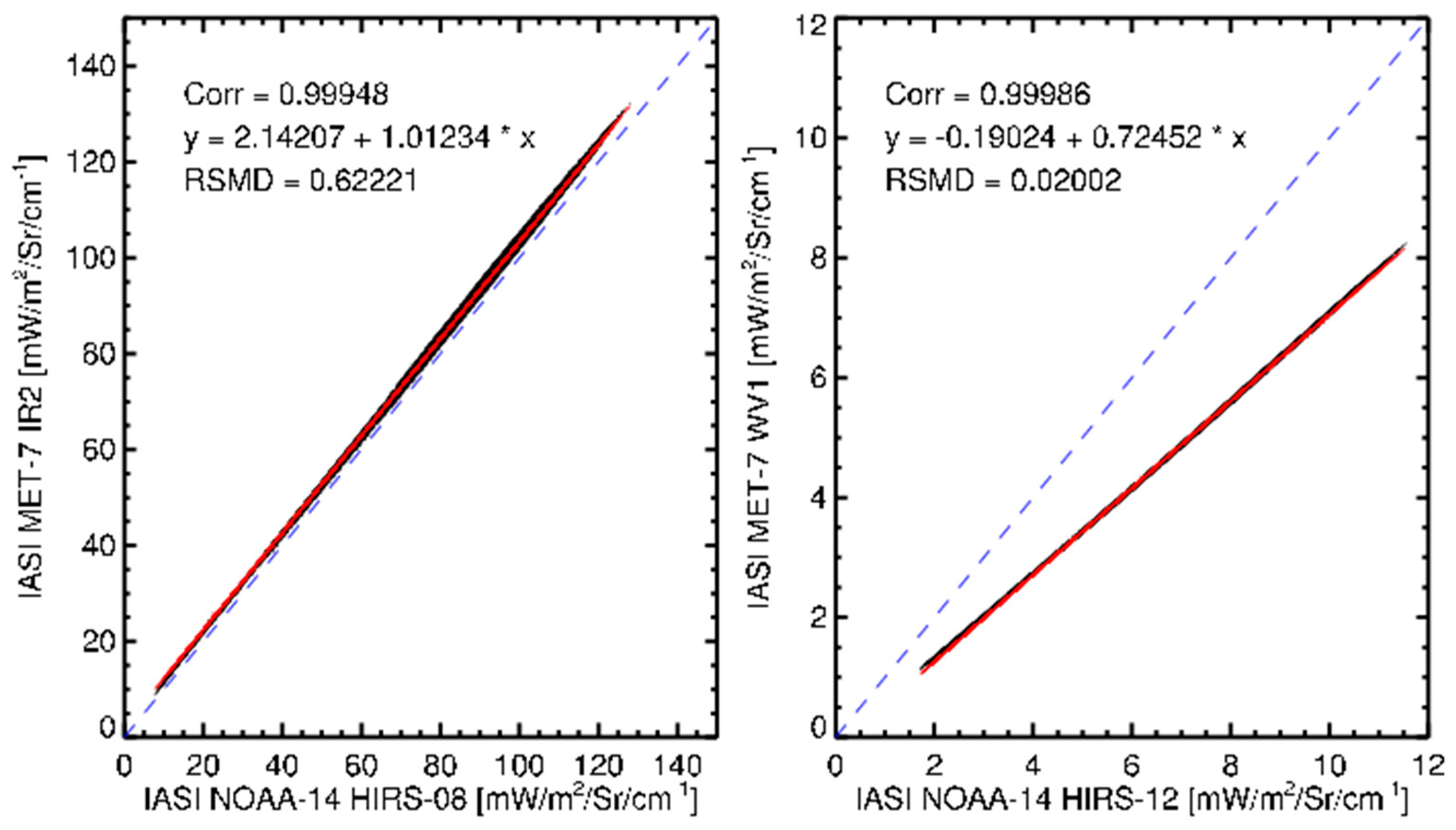
3.2.1. Spectral Band Adjustment for IASI

The measurements for the IASI hyperspectral sounder instrument had full spectral coverage for the IR and WV channels onboard the EUMETSAT and JMA geostationary satellites. Therefore, the reference radiance of a particular channel of the monitored instrument can be calculated by convolving the IASI spectra with the SRF of the IR or the WV channel.

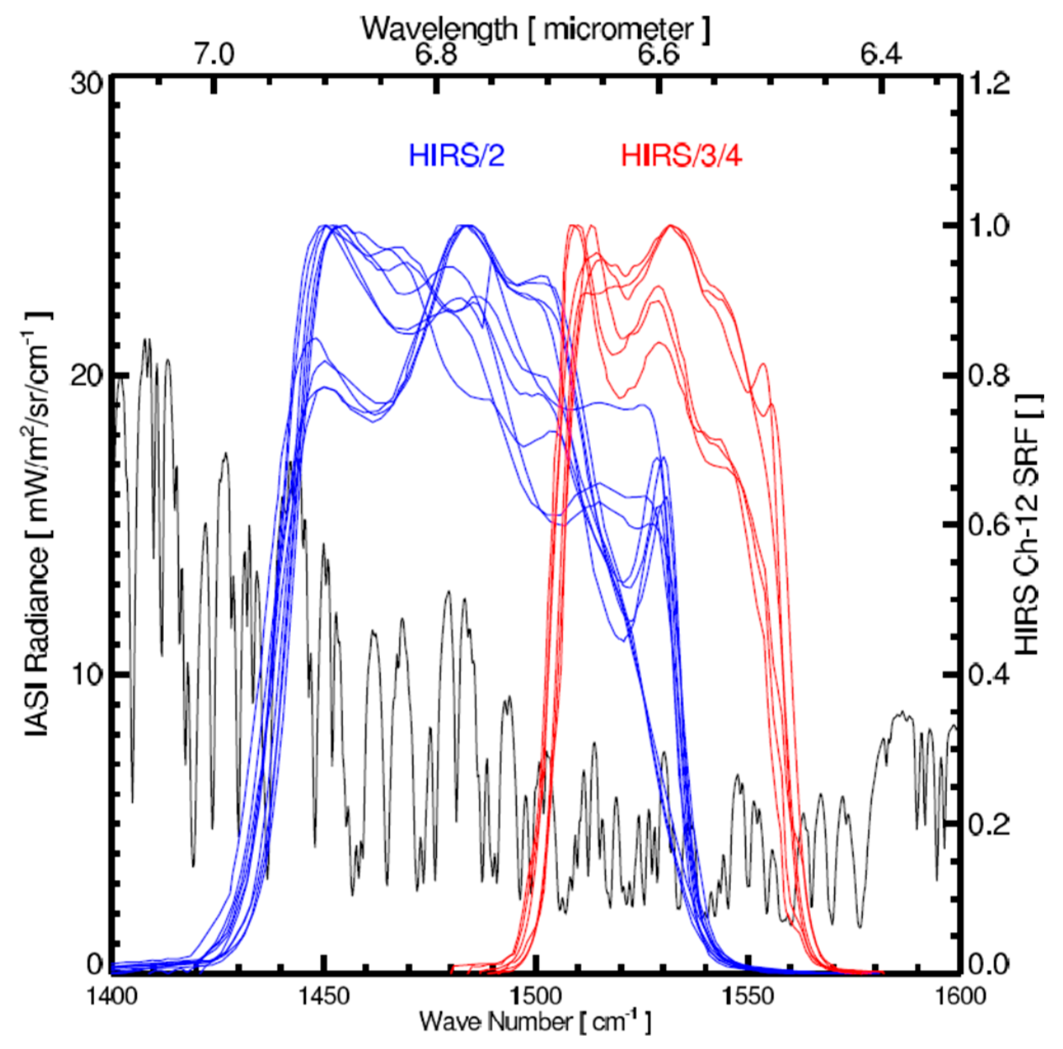
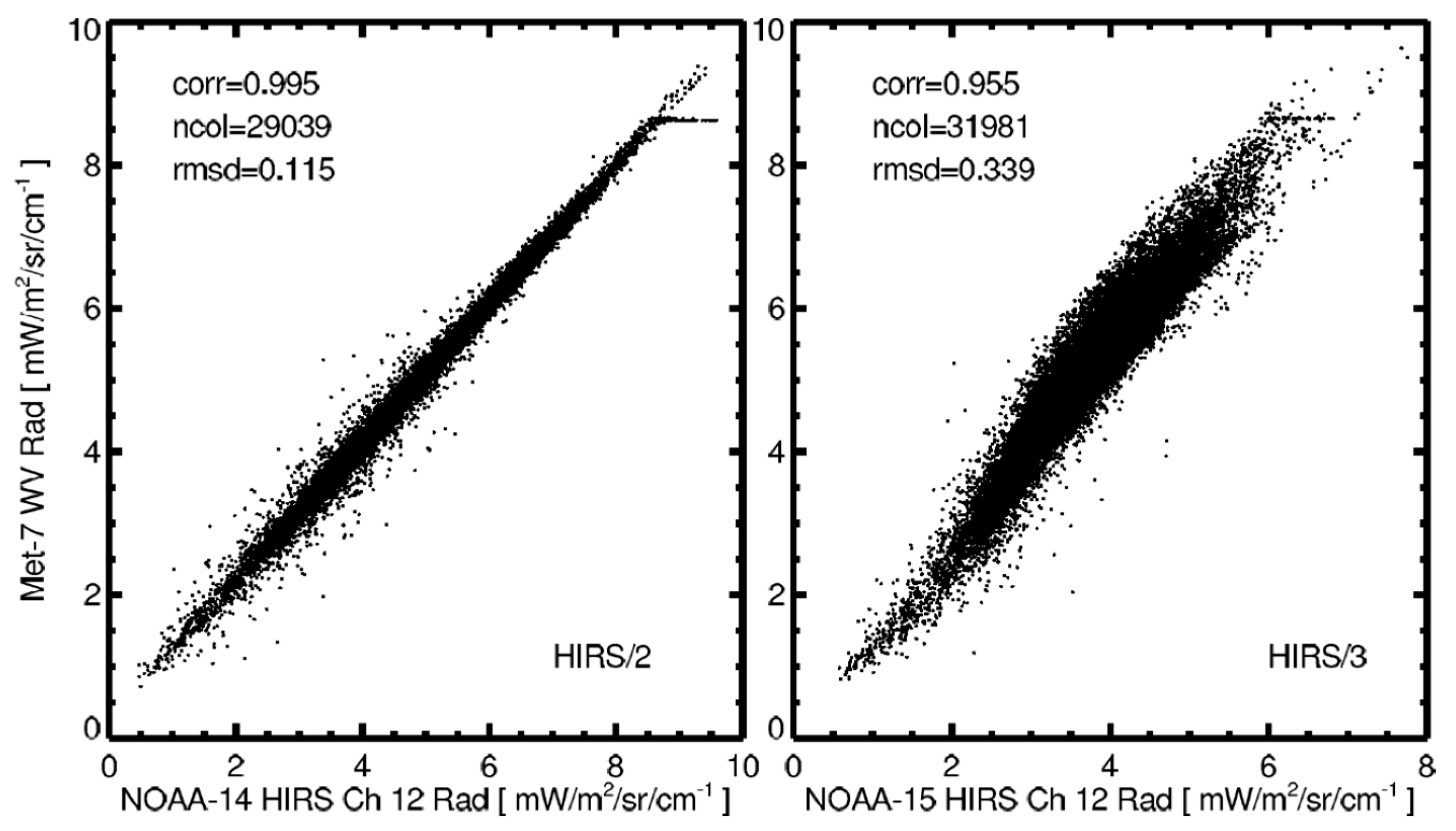
3.2.2. Spectral Band Adjustment for HIRS

The spectral conversion of broadband radiances provided by instruments such as HIRS is not trivial. A traditional way of computing the conversion factors or spectral band adjustment factors (SBAFs) is to find out the linear relationship between the broadband channel measurements using simulated radiances from an atmospheric profile dataset by using a radiative transfer model [9,18,19]. There are two main shortcomings in this approach: (1) the profile dataset is not capturing the real atmospheric variability, and (2) the radiative transfer model is not able to simulate the actual radiances, especially in the presence of hydrometeors.
To overcome this, we use IASI spectra with a spectral resolution of 0.25 cm−1, to simulate both reference and monitored broadband radiances by convoluting the spectra with respective SRFs. In order to make sure the full atmospheric variability is captured, about 200 thousand IASI spectra from randomly selected full orbits (one per month) were chosen for a whole year, i.e., 12 orbits. These spectra were then convolved with SRFs of the monitored instrument and reference instrument to obtain simulated radiances. An example of deriving SBAF is shown in Figure 4, which shows a very robust linear relationship between NOAA-14 HIRS/2 Channel 8 or 12 radiances and Met-7 IR or WV channel radiances (both simulated from IASI spectra). The red line in the figure shows the linear fit, and the root mean square of the fit residual was 0.6 mW/m2/sr−1/cm−1 for the IR channel and 0.02 mW/m2/sr−1/cm−1 for the WV channel. The small RMSD values suggest that uncertainties in the fit parameters were very small. The uncertainties of the offset and slope were 0.00687 and 0.00007 for the IR channel and 0.00031 and 0.00005 for the WV channel, respectively. The linear fit for the WV channel shows that monitored and reference radiances can differ significantly due to differences in SRFs and confirms the importance of applying SBAFs. The SBAFs are computed for all possible monitored and reference satellite combinations and are used to convert HIRS radiances to equivalent Meteosat IR or WV channel radiances.

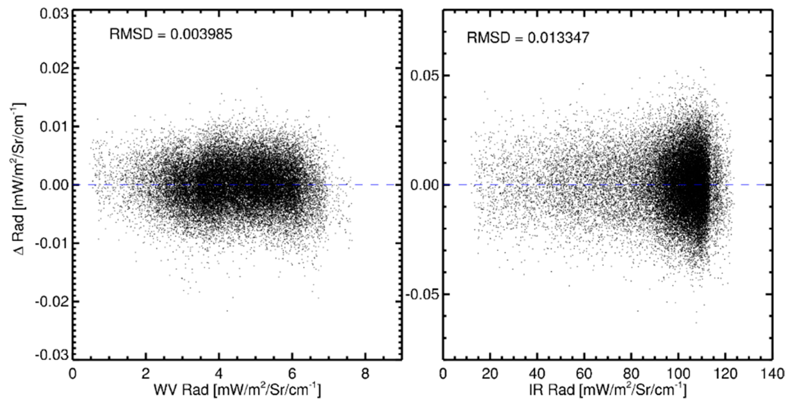
3.2.3. Spectral Band Adjustment for AIRS

Before using AIRS spectra for computation, they are checked for bad data using the quality flags that were provided with the data. AIRS channels having nonzero “CalChanSummary” flags were excluded. A flag value of zero means the channel was well calibrated for all scanlines in an AIRS 6-min granule; as such, a channel is referred below as a “good AIRS channel.”
The spectral gaps and popped channels, as discussed above, pose a significant problem for using AIRS spectra as a reference for recalibrating IR and WV channel measurements. The methods described in the literature for filling the gaps in the AIRS data use simulated measurements for the gaps and compromised channels taking model profiles including clouds as simulation input (see, for example, [18]). However, these methods, especially in the presence of clouds, are subject to significant uncertainties. Therefore, we decided to develop a method to compensate for the gaps and compromised channels, using IASI spectra instead of simulated spectra. Our method can be broken down into three steps:
(1)
We simulated the broadband measurements of IR and WV channels with the same set of IASI spectra as is used in the HIRS SBAF. We also simulated AIRS radiances by convolving the IASI spectra with AIRS channel SRFs.
(2)
We determined the predictors, which varied from granule to granule, to compute the simulated broadband radiances of IR and WV channels from the simulated “good AIRS channel” radiances (≈260 channels in the IR band and ≈210 channels in the WV band) using multiple linear regression.
(3)
We predicted the broadband radiances of IR and WV channels from real AIRS spectra by applying the predictors determined in Step 2.
Figure 5 demonstrates the robustness of the above described method, which revealed a very low root mean square difference (RMSD) between the broadband radiances computed from IASI measurements and the from available AIRS measurements. A comparison of our method against Tahara and Kato [18] for MTSAT/2 IMAGER IR and WV channels is presented in Section 5. The uncertainty of this method is less than the values reported in Reference [18].

3.3. Finding Match-Ups between Refernce and Monitored Measurements

The recalibration of Meteosat measurements was based on the comparison of these measurements (monitored measurements) to reference measurements from other satellite instruments. To facilitate such a comparison, both measurements would ideally be taken at the same time, sampling the same spatial area with the same viewing geometry. This was not possible in reality because of the way the different instruments make their measurements. The data from different instruments can only be collocated, in reality, by applying thresholds that define the maximum allowed differences in time and space, and for viewing conditions between the considered measurements. The thresholds were adapted from the GSICS methods as described in Hewison et al., (2013) [13]. A collocation represented a pair of measurements made by a reference instrument in low Earth orbit (LEO) and a geostationary (GEO) instrument, which have similar geographical, temporal and geometrical attributes. That is, they were measuring almost the same place at almost the same time and with almost the same viewing geometries. The collocations were found using an in-house developed algorithm. A set of observations from a pair of instruments within a common period (e.g., a day or a month) is required as input to the algorithm. The collocation algorithm involved the following steps: obtain data from both LEO and GEO instruments; select the relevant comparable portions and identify the pixels that were spatially collocated, temporally concurrent, geometrically aligned and spectrally compatible, and calculate the mean and variance of these counts or radiances; and write these information into files in NetCDF4 format.

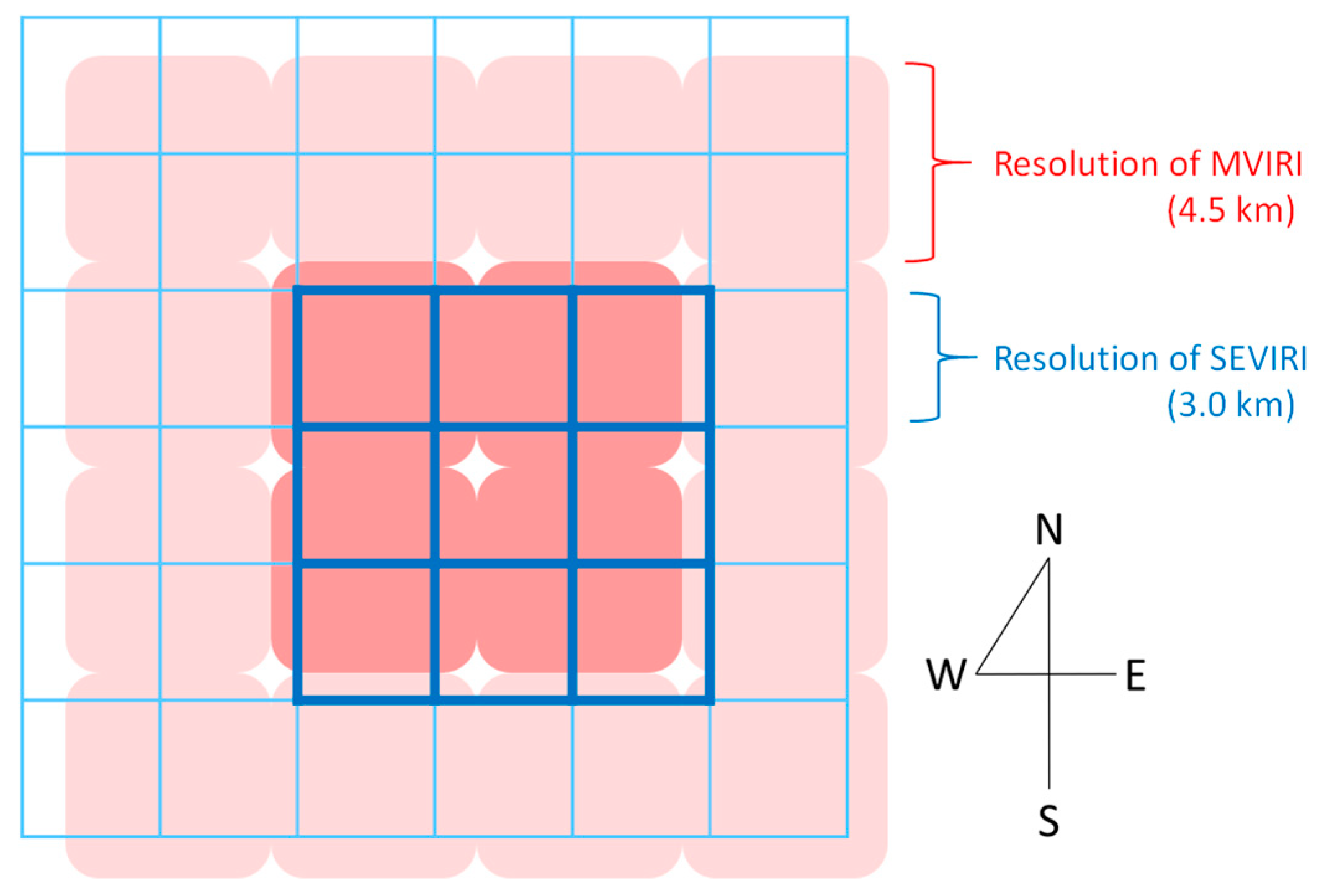
3.3.1. Collocation in Space

A target area was defined to be a little larger than the field of view (FoV) of the reference instruments similar to that described in Reference [13]. Thus, it covered all the contributing radiation and also considered small navigation errors, while being large enough to ensure reliable statistics of the spatial variance of the radiances. Although the exact ratio of the target area to the FoV was instrument-specific, it ranged in general between 1 and 3 times the FoV, with a minimum of 9 pixels from the monitored instrument.
For example, the MVIRI FoV was defined as square pixels with dimensions of 4.5 × 4.5 km at Sub Satellite Point (SSP). An array of 3 × 3 MVIRI pixels centered on the pixel closest to the centre of each reference pixel were taken to represent the collocation target area corresponding to the reference FoV. We also kept 5 × 5 MVIRI pixels’ statistics in the output file, which were used for additional checks in the variability.

3.3.2. Collocation in Time

Time stamps of the spatially collocated monitored geostationary (GEO) satellite measurements and reference low Earth orbit (LEO) measurements were compared. If the difference was greater than a threshold of 300 s, the collocation was rejected, otherwise it was retained for further processing [13,20].

3.3.3. Collocation in Viewing Geometry

The next step was to ensure that the spatially and temporally collocated measurements were observed under comparable geometrical conditions. This meant they should be aligned such that they view the surface at similar incidence angles, including azimuth and polarization, as well as elevation angles, through similar atmospheric paths.
Each pixel pair was tested sequentially to check whether the viewing geometries of the observations from both instruments were sufficiently close. The criterion for zenith angle was defined in terms of atmospheric path length, according to the difference in the secant of the observations’ zenith angles. If these were less than pre-determined thresholds, the collocated pixels were considered to be aligned in viewing geometry and included in further analysis. Otherwise they were rejected.
The geometric alignment of thermal infrared channels depended only on the zenith angle and not azimuth or polarisation, and was accepted when:
Δ θ = | c o s ( θ G E O )   c o s ( θ L E O ) 1 | <   θ m a x ,
where θ is the satellite viewing zenith angle. The threshold value for θ m a x   can be quite large for window channels (e.g., 0.05 for the IR channel), but must be rather small for more absorptive channels (e.g., <0.02 for WV channel). However, unless there are particular needs to increase the sample size for window channels, a common θ m a x   value of 0.01 may be used for all channels. For collocations between GEO and LEO satellites, this results in collocated measurements that are distributed approximately symmetrically around the equator, mapping out a characteristic slanted hourglass pattern. We limited the maximum incidence angle to 35° because it was observed that collocations with larger incidence angles introduced more noise.

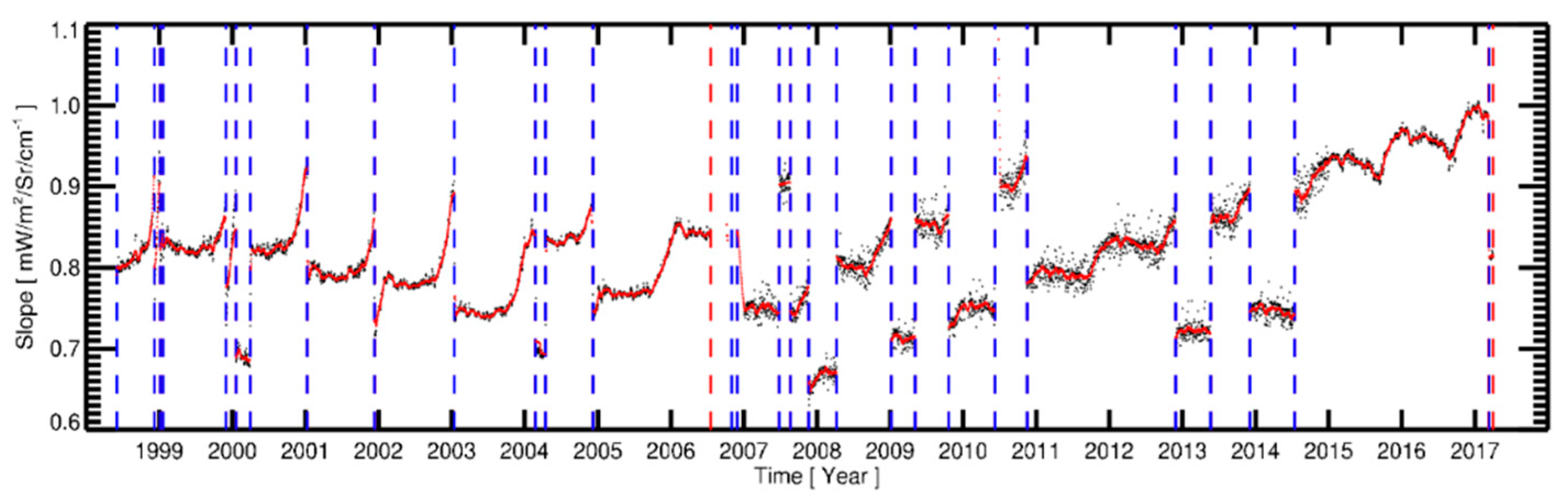
3.4. Determination of Calibration Coefficients

The recalibration coefficients were computed on a daily basis, but by collating 5 days of collocations, 2 days before and 2 days after. The coefficients were computed by regressing the measured counts from the monitored instrument (DN; digital number) with collocated and SBAF-applied radiances from the reference instrument. An example for collocation data for 5 days (±2 days for which the calibration coefficients were computed) is depicted in Figure 6. The x-axis represents an average (3 × 3) monitored counts and the y-axis represent pseudo-monitored radiances, i.e., the spectrally adjusted reference radiances. Each data point has uncertainties in both (x and y) axis directions. The uncertainties in the x-axis direction are defined by the variance of the 3 × 3 monitored counts. The uncertainties in the y-axis direction are a combination of uncertainties of the reference measurements (pre-launch determined noise equivalent radiance) and uncertainties of SBAFs. The linear regression used the method described in Press et al., (1992) [21], which took into account errors in both x and y, and therefore those collocations occurred under inhomogeneous conditions, represented by larger variance in the counts, got a smaller weight in the computation of calibration coefficients.
The calibration coefficients (offset, slope, and their corresponding uncertainties) were computed on a daily basis. From the black dots in Figure 7, it can be seen that day-to-day variations could be larger than expected. These variations were caused mainly by varying representativeness of the collocations to characterise the actual calibration of the instrument. To mitigate the effect of the day-to-day variations, we smoothed the parameters so that they represent gross changes in the calibration parameters between two radiometric events. The smoothing was achieved using a boxcar smoothing function of five-days width. If the neighbourhood around a point included a point outside the array, a mirrored edge point was used to compute the smoothed result. For example, when smoothing an n-element vector with a five-point-wide smoothing window, the second point of the result was equal to (A1 + A0 + A0 + A1 + A2)/5. These radiometric events (shown as dashed vertical lines in Figure 7) were gain setting changes of Meteosat-7 IR Channel. The gain levels were used to obtain the optimum dynamic range (0–255) for each spectral channel and were adjusted as required. The gain level adjustment was performed for compensating for the effects of radiometer contamination and detector ageing.
The users of the data can obtain recalibrated radiances for the IR and WV channels in mW/m2/sr/cm−1 according to Equations (2) and (3):
L i r = a i r + b i r × D N i r
L w v =   a w v   +   b w v ×   D N w v

3.5. Anchoring Recalibration Coefficients to a Prime Reference

The recalibration coefficients computed above may introduce systematic biases in the geostationary radiances due to systematic biases between the reference measurements that vary from one satellite to the other. In order to remove these biases between the reference measurements, all reference measurements were anchored to a prime reference satellite using the monitored measurements as bridges. Consider a1 and b1 as the offset and slope determined for a geostationary satellite using measurements from reference Satellite 1a2,b2 as the offset and slope determined for a geostationary satellite using measurements from reference Satellite 2. Recalibrated radiance corresponding to the geostationary measured counts can be obtained as:
L 1 = a 1 + b 1 × D N
L 2 =   a 2   +   b 2 ×   D N
Ideally, L1 and L2 will be the same, but due to potential biases in the reference measurements, L1 and L2 are not the same and the difference between the two can be approximated as the bias between the two reference measurements, assuming that the geostationary measurements do not have diurnally varying biases (this assumption is not valid particularly for three-axis-stabilised satellites [13]). If we assume Satellite 1 as the prime reference, L2 can be prime corrected as follows:
L1′2 = a1′2 + b1′2 × L2,
where the prime correction coefficients a1′2 and b1′2 are obtained via linear regression using L1 as the independent variable and L2 as the dependent variable by accumulating data for a common period where both Satellites 1 and 2 can be matched up against the same geostationary satellite. Here we assume that the biases of the individual satellites are time invariant, which may not be valid for all cases. One can also analytically determine the offset and slope of the prime correction as follows:
b1′2 = b1/b2
a1′2 = a1a2 × b1′2
The concept of prime correction is demonstrated using Aqua/AIRS as reference satellite 1, NOAA14/HIRS2 as reference Satellite 2 and GOES-9/Imager as the bridge geostationary satellite. GEOS-9/Imager was in operation from May 2003 till June 2005 over the western Pacific Ocean. The NOAA14/HIRS2 and Aqua/AIRS were in operation during the whole period. The red line and the blue line in Figure 8 represent the radiance of count 40 for the recalibrated GOES-9/Imager WV channel based on NOAA14/HIRS2 and Aqua/AIRS, respectively. There was a systematic difference between those two recalibrated radiances. For validation of the prime correction method, the correction parameters (as in Equations (7) and (8)) were estimated by using only a tiny fraction of the matchup data (highlighted by sky-blue colour). Those parameters were applied for the whole period of the recalibrated GOES-9/Imager WV channel radiance based on NOAA14/HIRS2, as shown by the pink line in Figure 8.
The prime correction method was also tested by using other geostationary satellites, i.e., Meteosat-5 and Meteosat-7, as bridges to prime correct NOAA-14/HIRS2 using Aqua/AIRS as the prime satellite. The test revealed that the impact of using another geostationary satellite as a bridge was small. The prime-corrected radiance corresponding to a radiance value of 5 mW/m2/sr/cm−1 was 5.19 ± 0.01 using Meteosat-5 and 5.21 ± 0.01 using Meteosat-7. The prime corrections could be taken back in time for a series of reference instruments using different or the same geostationary satellites as bridges. For example, radiances of Satellite 3 can be prime corrected to satellite 1 by prime correcting the radiance of Satellite 2 to Satellite 1 and then prime correcting Satellite 3’s radiance to Satellite 2. That means,
L1′3 = a1′2 + b1′2 × (a2′3 + b2′3 × L3)
and it can be repeated for n number of satellites to prime correct the nth satellite to the prime satellite 1. Metop-A/IASI was considered the “prime reference” and all other measurements were anchored to the prime reference measurements.

4. Validation

A common approach for the verification or validation of MVIRI IR and WV recalibrated radiances is presented. The improvements in the derived products are demonstrated by comparing the products derived using our recalibrated radiances to the products derived using operational radiances. The quality of the recalibrated radiances, which was generated with the methods presented in this paper, was evaluated in three papers. First, Govaerts et al., (2018) [22] demonstrated the improved identification of deep convective clouds by using the recalibrated IR radiances. Second, Bojanowski et al., (2018) [23] and Stockli et al., (2019) [24] used the recalibrated radiances for deriving cloud fractional cover climatology. Finally, Duguay-Tetzlaf et al., (2017) [25] demonstrated the impact of reduced bias and better temporal stability of the recalibrated radiances on their land surface temperature data record.
Tabata et al., (2019) [8] applied the method presented in this paper to recalibrate time-series of IR and WV radiances from JMA satellites and provides a detailed time series analysis of the of recalibrated radiances demonstrating the improvements to radiances and better stability in the time series. In this paper, therefore, we will not attempt to do a time series analysis of the recalibrated radiances. We will demonstrate the validity of the recalibrated radiances in two ways: comparing them to SEVIRI radiances and by comparing to GSICS corrected radiances where both of these measurements are considered as superior references compared to MVIRI measurements.

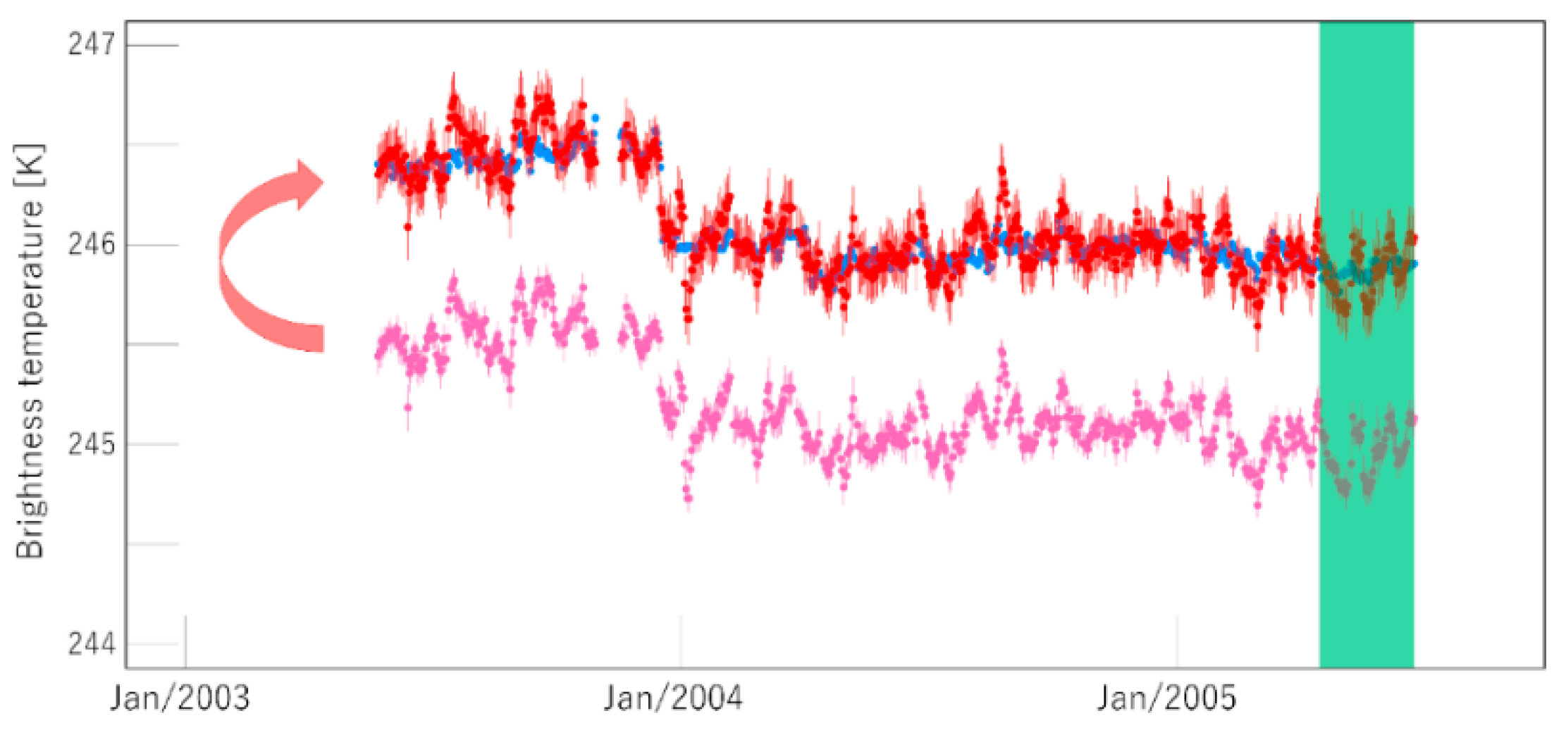
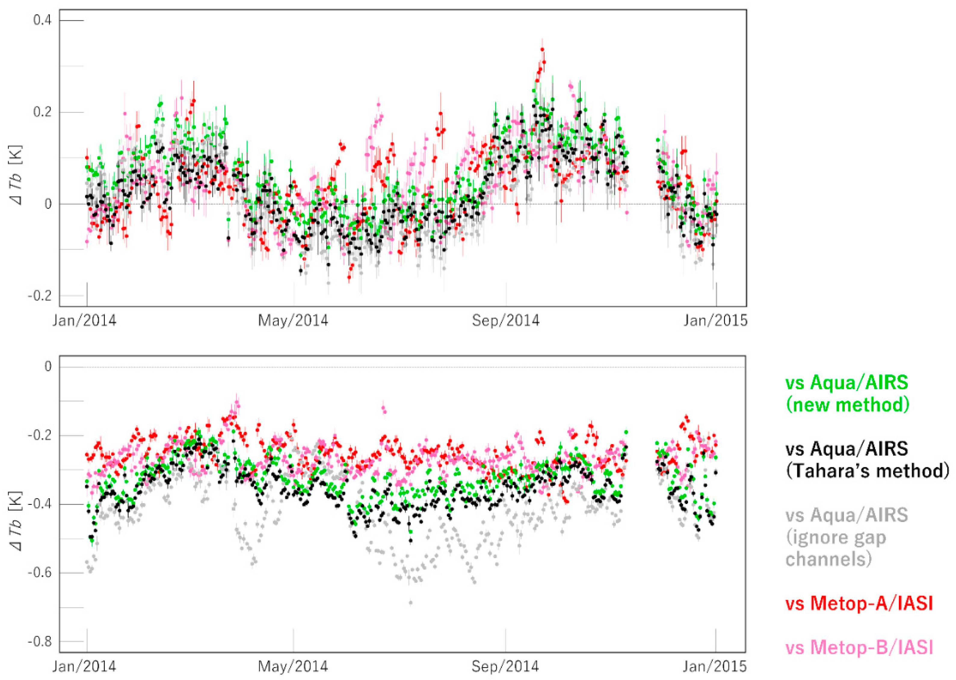
4.1. Comparison against Operational Calibrated and GSICS-Corrected Radiances

GSICS operationally provides corrections for the currently operating geostationary satellite measurements as described in Hewison et al., (2013) [13]. These corrections are available for Meteosat-7 since June 2008 until the end of the satellite operations. Figure 9 shows an example of the comparison between the recalibrated radiances based on the methods described in this paper and the corrected radiances based on the method used by GSICS (note that the GSICS correction for MFG was a demonstration product). In both cases, IASI measurements were used as the reference, but there were some differences in the methods, for example, GSICS uses only night-time overpasses of IASI (this was mainly to avoid solar contamination in the 3.9 micron channel) [13], whereas our method used both day and night overpasses. The GSICS correction was based on accumulating collocations for 29 days [13], whereas our method computed recalibration coefficients based on 5 days of collocations. In spite of these differences, it was encouraging to note that both methods give very similar results.
The mean and standard deviation of the operational calibrated, GSICS corrected and recalibrated time series shown are 92.00 ± 4.61, 96.46 ± 4.79 and 96.17 ± 4.81 mW/m2/sr/cm−1 for the IR channel and 4.65 ± 0.30, 4.23 ± 0.28 and 4.21 ± 0.28 mW/m2/sr/cm-1 for the WV channel, respectively. The relative differences between the operational calibrated and GSICS corrected radiances against our recalibrated radiances were 4.3% and 0.3% for the IR channel and 10.5% and 0.4% for the WV channel, respectively. This shows there were significant differences between the operational calibrated radiances and GSICS corrected or recalibrated radiances. The operational calibrated radiances were colder for the IR channel and warmer for the WV channel. The close agreement between the GSICS corrected and our recalibrated radiances warrants the validity of our recalibration method.

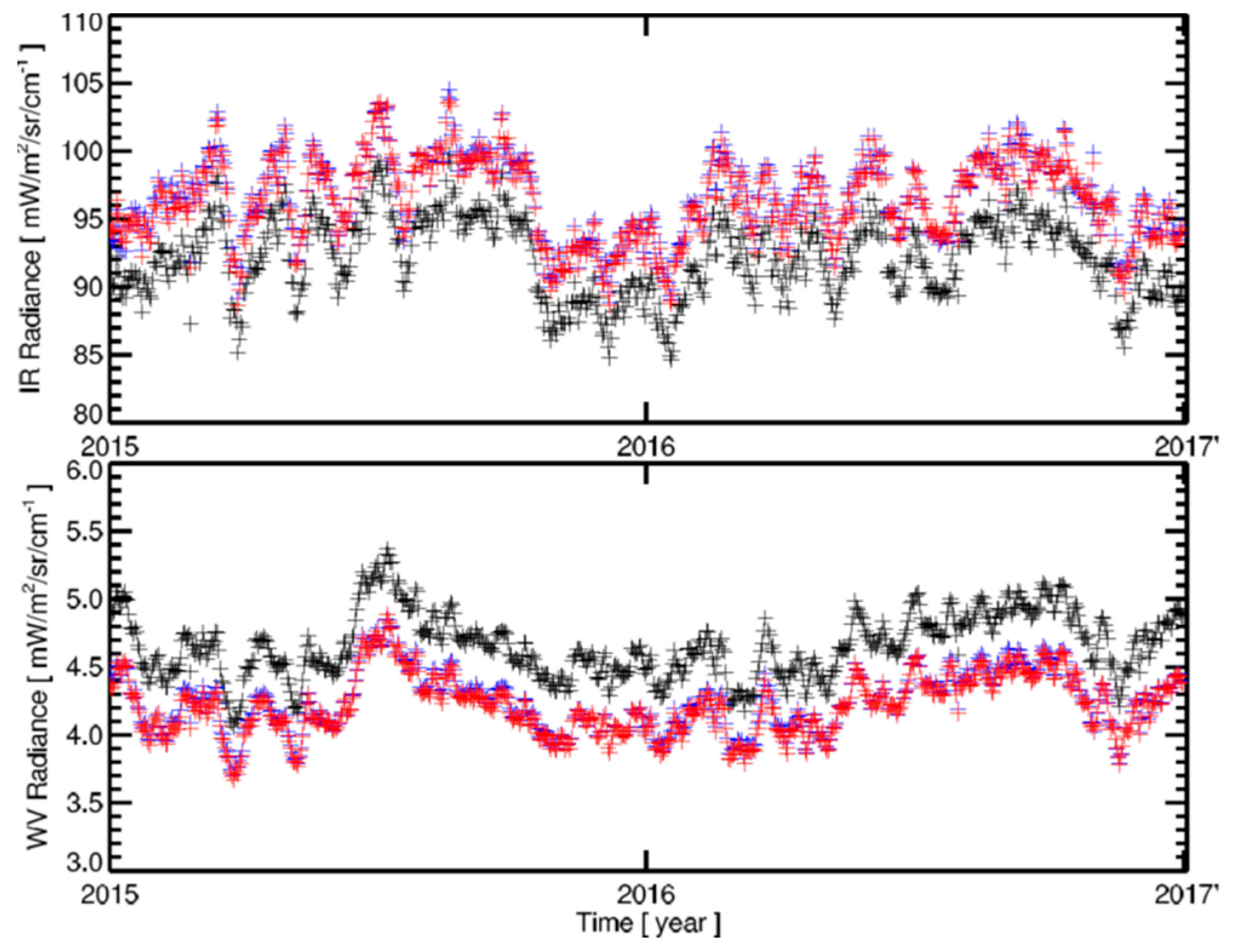
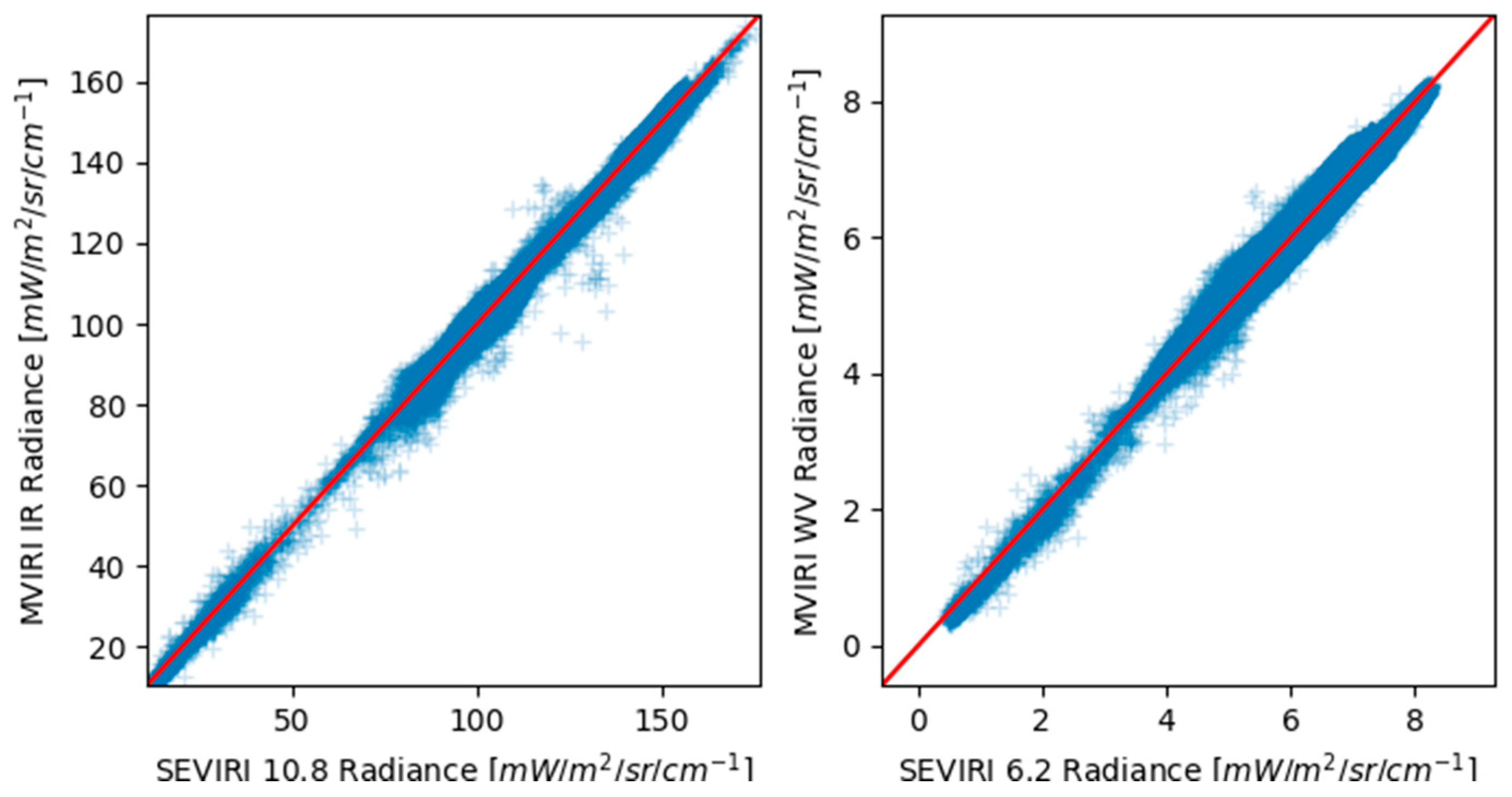
4.2. Comparison against SEVIRI Measurements

Meteosat-8, the first satellite in the MSG series was launched in August 2002 carrying the SEVIRI instrument. Since Meteosat-7 was nominally positioned at 0 degrees longitude and Meteosat-8 was nominally positioned at −3.4 degrees longitude, it is possible to compare the measurements of these two instruments. Observations from both instruments were rectified into a grid as if both instruments were viewing the Earth from 0 degrees longitude. The ground pixel resolutions of MVIRI and SEVIRI were different, with MVIRI pixels at the sub-satellite point having a sampling of 4.5 × 4.5 km2 and the SEVIRI pixels at the sub-satellite point having a sampling of 3 × 3 km2, as shown in Figure 10.
In order to have a similar spatial sampling, the 2 × 2 pixels of MVIRI and the 3 × 3 pixels of SEVIRI were averaged before comparing them. The temporal sampling rate of SEVIRI was double of that of MVIRI, where there are two MVIRI images and four SEVIRI images per hour. MVIRI imaging started at 00 and 30 min of the hour and it took about 25 min to finish an image. SEVIRI imaging started at 00, 15, 30 and 45 min of the hour and took about 12.5 min to finish an image. Provided that the imaging of both instruments started from the south-east corner of the disk, this implies that the 00-min image of the MVIRI will have temporal collocations with the 00-min SEVIRI image in the southern hemisphere and 15-min image in the northern hemisphere. Similarly, the 30-min image of the MIVIRI will have temporal collocations with the 30-min SEVIRI image in the southern hemisphere and the 45-min image in the northern hemisphere. Only those MVIRI and SEVIRI pixel averages were compared where the centre of the pixel averages, as shown in Figure 10, were less than 0.5 km apart and the temporal difference was less than 150 s. We also used another criterion to constrain the collocations, which was the product of the distance and time difference to be less than 10 km s. This criterion filtered out those collocations with large spatial and temporal differences, but allowed for keeping those ones with small temporal but with relatively large spatial differences and small spatial but relatively large temporal differences, and resulted in much less noise in the comparison results. For the viewing geometry, a threshold for the θ m a x value of 0.03 was used, where the θ m a x is defined in Equation (1).
An example of the MVIRI and SEVIRI comparison is shown in Figure 11. All collocations satisfying the above-mentioned criteria were further filtered for the scene homogeneity. The 3 × 3 SEVIRI pixels’ standard deviation was used as an indicator for the scene inhomogeneity. The thresholds used for filtering out inhomogeneous scenes were 0.3 and 1.2 mW/m2/sr/cm−1 for the WV and IR channels, respectively. Figure 11 shows the 393,720 collocations found for August 2004 after the filtering. MVIRI radiances were spectrally adjusted to match the SEVIRI measurements, the adjustment factors were computed as described in Section 3.2. The mean absolute difference between the measurements were 0.81 and 0.11 mW/m2/sr/cm−1 for the IR and WV channels, respectively. This corresponds to differences of 1% and 2%. These values were significantly smaller than the differences between operational calibrated radiances and recalibrated radiances shown in the previous section. This again illustrates the improvement of the recalibrated radiances over the operational calibrated radiances.

5. Discussion

Tahara et al., [18] presented a gap-filling method for overcoming AIRS spectral gaps in the spectral range of geostationary channels. They introduced virtual channels that compensate for the AIRS spectral gaps using simulated radiances for eight typical atmospheric profiles including clear and cloudy weather conditions over the tropics and mid latitudes. Their method did not rely on other satellite measurements compared to the gap filling method presented in this paper. One advantage of their method is that it can be applied to the shortwave infrared channel (≈3.7 µm), but its spectral regimes are not covered by the IASI measurements. However, this limitation is not important for our study because it targets only TIR channels. The advantage of the method presented in this paper is that it uses neither any atmospheric model nor a radiative transfer model, where both of them are known to have uncertainties.
Figure 12 top and bottom shows the biases of original MTSAT-2/IMAGER IR and WV channel radiance against Aqua/AIRS or Metop-A,B/IASI at standard radiance, respectively. The standard radiance is the typical radiance value calculated for the 1976 U.S. Standard Atmosphere for nadir condition in clear sky at night over an ocean surface with a sea surface temperature (SST) of 288.15 K and a wind speed of 7 m/s. The standard radiance of MTSAT-2/IMAGER IR and WV channel was 286.70 K and 239.1 K, respectively. The bias of the IR channel against Aqua/AIRS with the new method (green) was slightly larger than that with Tahara’s et al., method (black). The bias against AIRS that ignored gap-channels (grey, just convolution of available spectra) did not fit well with that against IASI (red and pink), especially in WV channel because there were non-negligible gaps in the spectral range of the SRF of the MTSAT-2/IMAGER WV channel. Note that this was before the prime reference correction. The systematic bias of SBAF applied reference measurements were removed by the prime reference correction.

6. Conclusions, Summary and Outlook

Over forty years in orbit, measurements from geostationary meteorological satellites offer immense potential for climate applications. However, the full potential of these measurements still cannot be exploited due to image and radiometric anomalies present in measured data. The international climate community has acknowledged the latter. Within the WMO initiative “Sustained and Coordinated Processing of Environmental Satellite data for Climate Monitoring (SCOPE-CM)”, a project (namely “Inter-calibration of imager observations from time-series of geostationary satellites (IOGEO)”) has been established to generate spatially and temporally (and spectrally, as an option) homogeneous radiance data from all geostationary satellites. To facilitate this, we have developed, in collaboration with the WMO supported initiative GSICS, a common baseline method that can be applied to recalibrate observations from heritage geostationary satellites.
This paper presents the description of approaches used in the common baseline method for recalibrating IR and WV channels onboard heritage geostationary satellites and demonstrates its validity though a validation for the IR and WV channels. The method relies on reference measurements and therefore the selection of suitable reference measurements is the first step. IASI, AIRS, and HIRS/2 were selected as reference instruments for the recalibration. The next step involved applying an approach that had been developed to spectrally modify the reference measurements so that they can be matched with the corresponding geostationary measurements. Hyperspectral measurements from IASI were used to compute SBAFs for HIRS broadband radiances and for handling spectral gaps in the AIRS measurements. It was shown that relying on high quality IASI measurements produces better results compared with previously employed radiative transfer model-based methods. Then, methods for collocating geostationary and reference measurements were adapted from Hewison et al., (2013) [13]. It was shown that the collocated measurements showed a robust linear relationship. These measurement pairs were linearly regressed to compute the recalibration coefficients. In order to correct for the systematic differences between the earlier reference measurements (e.g., HIRS or AIRS) and the Metop-A IASI hyperspectral reference measurements (the prime reference) our method adjusted earlier measurements to the prime reference using geostationary satellite measurements as a bridge. The calibration coefficients are available for every image of the considered instruments in this study. For the EUMETSAT satellites, EUMETSAT made these coefficients available in the MVIRI FCDR dataset, as well as in separate calibration files. For the JMA satellites, JMA made these coefficients available as separate calibration files [8].
Both the recalibration methods presented in this paper and the GSICS correction methods rely on reference measurements from polar orbiting satellites. These satellites, due to their sun-synchronous nature, measure the Earth twice daily, 12 h apart. Thus, it was not possible to collect collocated measurements from these polar satellites and geostationary satellites that covered the full diurnal cycle. This may not pose a significant issue for instruments onboard spinning satellites, such as MVIRI and SEVIRI, but could be an issue for instruments onboard three-axis stabilised satellites such as some JMA satellites. This required slight modification of the methods to incorporate onboard calibration targets for those satellites, as described in Tabata et al., (2019) [8].
The applicability of the methods presented in this paper is demonstrated in two ways for the MVIRI, SEVIRI, VISSR, JAMI, IMAGER and Imager instruments. First, by comparing the MVIRI recalibrated radiances with the GSICS-corrected MVIRI radiances. Second, by comparing MVIRI recalibrated radiances with SEVIRI radiances. Both comparisons show that presented methods could correct for radiometric anomalies in the operational radiances. Compared to the operational radiances, significant reduction in biases were observed for both IR and WV channels, of 4% and 10%, respectively. The mean absolute difference between recalibrated radiances and SEVIRI radiances were 0.81 and 0.11 mW/m2/sr/cm−1 for the IR and WV channels, respectively. This corresponds to differences of 1% and 2%, respectively. These values are significantly smaller than the differences between operational calibrated radiances and recalibrated radiances.
Further, radiances recalibrated with the methods presented in this paper were used in several studies [22,23,24,25] that showed their superiority to operational calibrated radiances. Finally, Tabata et al., (2019) [8] presented a comprehensive validation a full time-series, covering the years 1978–2016, of recalibrated IR and WV radiances from the VISSR, JAMI, IMAGER and Imager instruments onboard JMA’s geostationary satellites (paper has been submitted to the same special issue as this paper). In their paper, they show that their recalibrated radiances were radiometrically superior to their operational calibrated data and that the time series showed better intersatellite agreement and stability. A similar paper on the time series analysis of MVIRI and SEVIRI data is being prepared.
This study only deals with the radiometric anomalies in the operational calibrated data. However, there are known image anomalies (e.g., Köpken [26]) and those need to be accounted for as well. EUMETSAT has already made an effort to detect and flag such anomalies in the whole archive of MVIRI measurements and a paper is being prepared on the methods for the detection and on the statistics of various anomalies in the MVIRI measurements.

Author Contributions

Conceptualization, all authors.; data curation, V.O.J. for EUM data and T.T. for JMA data; formal analysis, V.O.J. and T.T.; investigation, V.O.J. and T.T.; methodology, all authors; project administration, R.R. and J.S.; software, V.O.J. and T.T.; supervision, R.R., T.H. and J.S.; validation, V.O.J., T.T. and F.R.; visualization, V.O.J., T.T. and F.R.; writing—original draft preparation, V.O.J., writing—review and editing, all authors.

Funding

This research was funded by EUMETSAT and TT was funded by JMA and a Fellowship Program by the Ministry of Education, Culture, Sports, Science and Technology of the Japanese Government and supported by EUMETSAT through a visiting scientist activity at EUMETSAT.

Acknowledgments

The authors would like to thank EUMETSAT NWP SAF for the RTTOV radiative transfer model, AIRS team for AIRS data and NOAA for HIRS data.

Conflicts of Interest

The authors declare no conflict of interest.

Abbreviations

The following abbreviations are used in this manuscript:
AIRSAtmospheric Infrared Sounder
DNDigital Number
EUMETSATEuropean Organisation for the Exploitation of Meteorological Satellites
FCDRFundamental Climate Data Record
FoRField of Regard
FoVField of View
GCOSGlobal Climate Observing System
GEOGeostationary
GMSGeostationary Metrological Satellite
GOESGeostationary Operational Environmental Satellite system
GSICSGlobal Space-Based Inter-Calibration System
HIRSHigh Resolution Infrared Radiation Sounder
IASIInfrared Atmospheric Sounding Interferometer
IOGEOInter-Calibration of Imager Observations from Time-Series of Geostationary Satellites
IRInfrared
JAMIJapanese Advanced Meteorological Imager instrument
JMAJapan Meteorological Agency
LEOLow Earth Orbit
MFGMeteosat First Generation
MVIRIMeteosat Visible and InfraRed Imager
MSGMeteosat Second Generation
MSICCMulti Sensor Infrared Channel Calibration
MTSATMulti-Functional Transport Satellite
MVIRIMeteosat Visible and Infrared Imager (onboard MFG satellites)
NASANational Aeronautics and Space Administration
NCEPNational Centers for Environmental Prediction
NOAANational Oceanic and Atmospheric Administration
OSCARObserving Systems Capability Analysis and Review Tool
REFReference
RMSDRoot Mean Square Difference
RTTOVRadiative Transfer for TOVS
SBAFSpectral Band Adjustment Factor
SCOPE-CMSustained and Coordinated Processing of Environmental Satellite Data for Climate Monitoring
SEVIRISpinning Enhanced Visible and Infrared Imager (onboard MSG satellites)
SNRSignal to Noise Ratio
SRFSpectral Response Function
SSPSub-Satellite Point
SSTSea Surface Temperature
TIRThermal Infrared
TIROSTelevision Infrared Observation Satellite
TOVSTIROS Operational Vertical Sounder
VISSRVisible and Infrared Spin Scan Radiometer
WMOWorld Meteorological Organization
WVWater Vapour

References

  1. Schmetz, J.; Menzel, W.P. A Look at the Evolution of Meteorological Satellites: Advancing Capabilities and Meeting User Requirements. Weather Clim. Soc. 2015, 7, 309–320. [Google Scholar] [CrossRef]
  2. GCOS. The Global Observing System for Climate: Implementation Needs. 2016. Available online: https://ane4bf-datap1.s3-eu-west-1.amazonaws.com/wmocms/s3fs-public/programme/brochure/GCOS-200_OnlineVersion.pdf?PlowENiCc1RGh9ReoeAoGBT0QhnJYm6_ (accessed on 7 November 2018).
  3. Schmetz, J. Operational calibration of the METEOSAT water vapor channel by calculated radiances. Appl. Opt. 1989, 28, 3030–3038. [Google Scholar] [CrossRef]
  4. Van de Berg, L.C.J.; Schmetz, J.; Whitlock, J. On the calibration of the Meteosat water vapor channel. J. Geophys. Res. 1995, 100, 21069–21076. [Google Scholar] [CrossRef]
  5. Gube, M.; Gaertner, V.; Schmetz, J. Analysis of the Operational Calibration of the Meteosat Infrared-Window Channel. Meteorol. Appl. 1996, 3, 307–316. [Google Scholar] [CrossRef]
  6. Weinreb, M.; Jamieson, M.; Fulton, N.; Chen, Y.; Johnson, J.X.; Bremer, J.; Smith, C.; Baucom, J. Operational calibration of Geostationary Operational Environmental Satellite-8 and -9 imagers and sounders. Appl. Opt. 1997, 36, 6895–6904. [Google Scholar] [CrossRef] [PubMed]
  7. Tokuno, M.; Itaya, H.; Tsuchiya, K.; Kurihara, S. Calibration of VISSR on board GMS-5. Adv. Space Res. 1997, 19, 1297–1306. [Google Scholar] [CrossRef]
  8. Tabata, T.; John, V.O.; Roebeling, R.A.; Hewison, T.; Schulz, J. Recalibration of over 35 years of infrared and water vapor channel radiances of the JMA geostationary satellites. Remote Sens. under review.
  9. Tjemkes, S.A.; König, M.; Lutz, H.-J.; van de Berg, L.; Schmetz, J. Calibration of Meteosat water vapor channel observations with independent, satellite observations. J. Geophys. Res. 2001, 106, 5199–5209. [Google Scholar] [CrossRef]
  10. Brogniez, H.; Roca, R.; Picon, L. A clear-sky radiance archive from METEOSAT ‘water vapor’ observations. J. Geophys. Res. 2006, 111, D21109. [Google Scholar] [CrossRef]
  11. Rosema, A.; Foppes, S.; van der Woerd, J. Meteosat Derived Planetary Temperature Trend 1982–2006. Energy Environ. 2013, 24, 381–395. [Google Scholar] [CrossRef]
  12. Goldberg, M.; Ohring, G.; Butler, J.; Cao, C.; Datla, R.; Doelling, D.; Gaertner, V.; Hewison, T.; Iacovazzi, B.; Kim, D.; et al. The global space-based inter-calibration system (GSICS). Bull. Am. Meteorol. Soc. 2011, 92, 468–475. [Google Scholar] [CrossRef]
  13. Hewison, T.J.; Wu, X.; Yu, F.; Tahara, Y.; Hu, X.; Kim, D.; Koenig, M. GSICS Inter-Calibration of Infrared Channels of Geostationary Imagers using Metop/IASI. IEEE Trans. Geosci. Remote Sens. 2013, 51, 3. [Google Scholar] [CrossRef]
  14. Schmetz, J.; Pili, P.; Tjemkes, S.; Just, D.; Kerkmann, J.; Rota, S.; Ratier, A. An Introduction to Meteosat Second Generation (MSG)—and supplements. Bull. Am. Meteor. Soc. 2002, 83, 977–992. [Google Scholar] [CrossRef]
  15. JMA. Preliminary Validation Report on MTSAT-1R Imagery Data, CGMS33 JMA-WP-11. In Proceedings of the 33th Meeting of the Coordination Group for Meteorological Satellites (CGMS), Tokyo, Japan, 1–4 November 2005. [Google Scholar]
  16. Hilton, F.; Armante, R.; August, T.; Barnet, C.; Bouchard, A.; Camy-Peyret, C.; Capelle, V.; Clarisse, L.; Clerbaux, C.; Coheur, P.F.; Collard, A. Hyperspectral Earth observation from IASI: Five years of accomplishments. Bull. Am. Meteor. Soc. 2012, 93, 347–370. [Google Scholar] [CrossRef]
  17. Shi, L.; Bates, J.; Shi, L. Three decades of intersatellite-calibrated High-Resolution Infrared Radiation Sounder upper tropospheric water vapour. J. Geophys. Res. 2011, 116, D04108. [Google Scholar] [CrossRef]
  18. Tahara, Y.; Koji, K. New Spectral Compensation Method for Intercalibration Using High Spectral Resolution Sounder. Meteorol. Satell. Cent. Tech. Note 2009, 52, 1–37. [Google Scholar]
  19. Knapp, K.R. Calibration Assessment of ISCCP Geostationary Infrared Observations Using HIRS. J. Atmos. Ocean. Technol. 2008, 25, 183–195. [Google Scholar] [CrossRef]
  20. John, V.O.; Holl, G.; Buehler, S.A.; Candy, B.; Saunders, R.W.; Parker, D.E. Understanding intersatellite biases of microwave humidity sounders using global simultaneous nadir overpasses. J. Geophys. Res. 2012, 117, D02305. [Google Scholar] [CrossRef]
  21. Press, W.H.; Teukolksy, S.; Vetterling, W.T.; Flannery, B. Numerical Recipes in FORTRAN 77: The Art of Scientific Computing, 2nd ed.; Cambridge University Press: Cambridge, UK, 1992. [Google Scholar]
  22. Govaerts, Y.M.; Rüthrich, F.; John, V.O.; Quast, R. Climate Data Records from Meteosat First Generation Part I: Simulation of Accurate Top-of-Atmosphere Spectral Radiance over Pseudo-Invariant Calibration Sites for the Retrieval of the In-Flight Visible Spectral Response. Remote Sens. 2018, 10, 1959. [Google Scholar] [CrossRef]
  23. Bojanowski, J.S.; Stöckli, R.; Duguay-Tetzlaff, A.; Finkensieper, S.; Hollmann, R. Performance Assessment of the COMET Cloud Fractional Cover Climatology across Meteosat Generations. Remote Sens. 2018, 10, 804. [Google Scholar] [CrossRef]
  24. Stöckli, R.; Bojanowski, J.S.; John, V.O.; Duguay-Tetzlaff, A.; Bourgeois, Q.; Schulz, J.; Hollmann, R. Cloud Detection with Historical Geostationary Satellite Sensors for Climate Applications. Remote Sens. 2019, 11, 1052. [Google Scholar] [CrossRef]
  25. Duguay–Tetzlaff, A.; Stöckli, R.; Bojanowski, J.; Hollmann, R.; Fuchs, P.; Werscheck, M. CM SAF Land SUrface Temperature Dataset from METeosat First and Second Generation, 1st ed.; Satellite Application Facility on Climate Monitoring: Offenbach, Germany, 2017. [Google Scholar]
  26. Köpken, C. Solar Stray Light Effects in Meteosat Radiances Observed and Quantified Using Operational Data Monitoring at ECMWF. J. Appl. Meteor. 2004, 43, 28–37. [Google Scholar] [CrossRef]
Figure 1. Spectral response functions for (top) IR and (bottom) WV channels on EUMETSAT and JMA geostationary satellites considered in this study. Infrared Atmospheric Sounding Interferometer (IASI) spectra are also shown to illustrate atmospheric opaqueness at these spectral regimes. Brown dots represents spectral sampling of Atmospheric Infrared Sounder (AIRS) measurements. Two small gaps in the AIRS spectra are visible in the IR channel spectral range, but there are large gaps in the WV spectral range, which requires some additional processing before these spectra can be used for the recalibration of IR and WV channel measurements.
Remotesensing 11 01171 g001
Figure 2. Spectral response functions of HIRS/2 (blue), HIRS/3 (red) and HIRS/4 (red) instruments for the Channel 12 (≈6 µm). IASI spectra (black) are also shown to illustrate atmospheric opaqueness for these spectral regimes. The approximate spectral ranges for the HIRS/2 series and the HIRS/3 and HIRS/4 series are marked at the top, which clearly indicates a spectral shift between the generations. Satellites carrying HIRS/2 instruments are TIROS-N and NOAA-6 through NOAA-14. Satellites carrying HIRS/3 instruments are NOAA-15 through NOAA-17. Satellites carrying HIRS/4 instruments are NOAA-18, NOAA-19, Metop-A and Metop-B.
Remotesensing 11 01171 g002
Figure 3. Impact of Channel 12 SRF changes between HIRS/2 and HIRS/3/4 on the collocation uncertainties with MVIRI WV channel. Collocations are for January 2003, see text for more details.
Remotesensing 11 01171 g003
Figure 4. Example of deriving spectral band adjustment factors (SBAF). A linear fit between the two radiances are shown using the red line. There were 202,477 data points that were used to determine the linear fit parameters.
Remotesensing 11 01171 g004
Figure 5. Demonstration of constructing broadband radiances from available AIRS channels. The plots show the difference between the Meteosat-7 radiances computed from available AIRS channels and from the full IASI spectra for the WV (left) and IR (right) channels.
Remotesensing 11 01171 g005
Figure 6. Regression between MVIRI measured counts and pseudo-MVIRI radiances computed from collocated IASI spectra, which were used to compute calibration coefficients. Errors in both the counts and pseudo-radiances were used to compute the linear fit (red line) parameters. Calibration coefficients were computed per day by collating 5 days of matchups (±2 days).
Remotesensing 11 01171 g006
Figure 7. Time series of calibration slope for Meteosat-7 IR channel. Vertical dashed lines represent radiometric events such as gain changes. The vertical dashed red line shows the start of the satellite’s move to the Indian Ocean and also the end of the life time. Black dotted lines represent daily calibration values and the red lines are the smoothed calibration values, which will be used for the recalibration.
Remotesensing 11 01171 g007
Figure 8. Recalibrated radiances equivalent to count 40 of GOES-9/Imager WV channel derived from recalibration coefficients by Aqua/AIRS (blue) and those by NOAA-14/HIRS2 (pink), and the prime corrected NOAA-14/HIRS2 (red) using Aqua/AIRS as the prime satellite. The green shaded region represents the period where data was used to compute the prime correction parameters.
Remotesensing 11 01171 g008
Figure 9. Comparison of operational calibrated (black), GSICS corrected (blue) and recalibrated (red) radiances for IR (top) and WV (bottom) channel measurements (see text for details). Measurements from noon images with viewing zenith angles less than 60 degree were used in this figure.
Remotesensing 11 01171 g009
Figure 10. Schematic of the MVIRI (2 × 2 red boxes) and SEVIRI (3 × 3 boxes with blue borders) pixel averages used for the comparison.
Remotesensing 11 01171 g010
Figure 11. Results of the comparison between MVIRI and SEVIRI recalibrated measurements for August 2004. As discussed in the text, the collocations were in the southern hemisphere. The SEVIRI measurements were spectrally adjusted to MVIRI measurements, as described in Section 3.2.
Remotesensing 11 01171 g011
Figure 12. Bias of original MTSAT-2/IMAGER IR (top) and WV (bottom) channel radiance against Aqua/AIRS or Metop-A,B/IASI at standard radiance. Note that during the gap that is seen in November, MTSAT-1R was the operational satellite.
Remotesensing 11 01171 g012
Table 1. Spatial, temporal, spectral and radiometric characteristics of IR and WV channels that are considered in this study. The signal to noise ratio (SNR) values are taken from the WMO OSCAR database and CGMS working paper [15], which are nominal values determined prelaunch, but may not match with the actual radiometric noise of the measurements.
ChannelSpatial Sampling at Nadir (km)Central Wavelength (µm)SNR (K)
MVIRI (Meteosat-2, -3, -4, -5, -6, -7); 1981–2017
WV5.06.41.00 K @ 250 K
IR5.011.50.50 K @ 300 K
SEVIRI (Meteosat-8, -9, -10, -11); 2003–
WV3.06.250.75 K @ 250 K
IR3.010.80.25 K @ 300 K
VISSR (GMS, GMS-2, -3, -4); 1978–1995
IR5.011.5≤0.5 K @ 300 K
VISSR (GMS-5); 1995–2003
WV5.06.75≤0.22 K @ 300 K
IR5.011.0≤0.35 K @ 300 K
JAMI (MTSAT-1R); 2005–2014
WV4.06.750.15 K @ 300 K
IR4.010.80.18 K @ 300 K
IMAGER (MTSAT-2); 2009–2016
WV4.06.750.11 K @ 300 K
IR4.010.80.12 K @ 300 K
Imager (GOES-9); 2003–2005
WV8.06.750.09 K @ 300 K
IR4.010.70.11 K @ 300 K

