Article

Quantitative Assessment of the Impact of Physical and Anthropogenic Factors on Vegetation Spatial-Temporal Variation in Northern Tibet

1
University of Chinese Academy of Sciences, Beijing 100049, China
2
CAS Center for Excellence in Tibetan Plateau Earth Sciences, Chinese Academy of Sciences (CAS), Beijing 100101, China
3
State Key Laboratory of Remote Sensing Science, Institute of Remote Sensing and Digital Earth, Chinese Academy of Sciences, Beijing 100101, China
4
ICube Laboratory, UMR 7357 CNRS-University of Strasbourg, 300 bd Sebastien Brant, CS 10413, F-67412 Illkirch CEDEX, France
5
Research Network of Global Change Biology, Beijing Institutes of Life Science, Chinese Academy of Sciences, Beijing 100101, China
*
Author to whom correspondence should be addressed.
Remote Sens. 2019, 11(10), 1183; https://0-doi-org.brum.beds.ac.uk/10.3390/rs11101183
Submission received: 7 March 2019 / Revised: 12 May 2019 / Accepted: 14 May 2019 / Published: 18 May 2019

Abstract

:
The alpine grassland on the Qinghai-Tibet Plateau covers an area of about 1/3 of China’s total grassland area and plays a crucial role in regulating grassland ecological functions. Both environmental changes and irrational use of the grassland can result in severe grassland degradation in some areas of the Qinghai-Tibet Plateau. However, the magnitude and patterns of the physical and anthropogenic factors in driving grassland variation over northern Tibet remain debatable, and the interactive influences among those factors are still unclear. In this study, we employed a geographical detector model to quantify the primary and interactive impacts of both the physical factors (precipitation, temperature, sunshine duration, soil type, elevation, slope, and aspect) and the anthropogenic factors (population density, road density, residential density, grazing density, per capita GDP, and land use type) on vegetation variation from 2000 to 2015 in northern Tibet. Our results show that the vegetation index in northern Tibet significantly decreased from 2000 to 2015. Overall, the stability of vegetation types was sorted as follows: the alpine scrub > the alpine steppe > the alpine meadow. The physical factors, rather than the anthropogenic factors, have been the primary driving factors for vegetation dynamics in northern Tibet. Specifically, meteorological factors best explained the alpine meadow and alpine steppe variation. Precipitation was the key factor that influenced the alpine meadow variation, whereas temperature was the key factor that contributed to the alpine steppe variation. The anthropogenic factors, such as population density, grazing density and per capita GDP, influenced the alpine scrub variation most. The influence of population density is highly similar to that of grazing density, which may provide convenient access to simplify the study of the anthropogenic activities in the Tibet plateau. The interactions between the driving factors had larger effects on vegetation than any single factor. In the alpine meadow, the interaction between precipitation and temperature can explain 44.6% of the vegetation variation. In the alpine scrub, the interaction between temperature and GDP was the highest, accounting for 27.5% of vegetation variation. For the alpine steppe, the interaction between soil type and population density can explain 29.4% of the vegetation variation. The highest value of vegetation degradation occurred in the range of 448–469 mm rainfall in the alpine meadow, 0.61–1.23 people/km2 in the alpine scrub and –0.83–0.15 °C in the alpine steppe, respectively. These findings could contribute to a better understanding of degradation prevention and sustainable development of the alpine grassland ecosystem in northern Tibet.

Graphical Abstract

1. Introduction

As the main terrestrial ecosystem in the Qinghai-Tibet Plateau, grassland ecosystems are vulnerable to external disturbances and sensitive to environmental changes [1]. In recent years, grassland ecosystems in the Qinghai-Tibet Plateau have faced different degrees of degradation [2]. Both physical and anthropogenic factors (e.g., climate, soil type, topography, population, grazing density and land use [3,4,5,6,7,8]) are considered major driving forces of vegetation variation. Previous studies have analyzed the individual contribution of each physical or anthropogenic factor to variation in vegetation cover through the analysis of correlation and regression coefficients [9,10]. However, the primary and potential interactive or combined impacts of both physical and anthropogenic factors on vegetation variation still remain unclear.
A large number of studies have dedicated enormous efforts to analyze the causes of vegetation variation. In particular, numerous studies have analyzed the relationships between vegetation index and meteorological factors [11,12,13,14,15]. For example, precipitation and temperature have been reported as the main factors affecting variations in grassland vegetation cover in the Qinghai-Tibet plateau [16,17,18]. Some researches have denoted that environmental humidity conditions (precipitation, vapor pressure, and relative humidity) dominate the vegetation index variation over the Tibetan plateau [19]. Still, other studies have indicated that physical factors, such as soil types, solar radiation and elevation, play important roles in vegetation cover change. Soil types determine different water retention and venting properties, and are found to significantly modulate the vegetation trends in dry land [20]. Solar radiation is the dominant controller of plant photosynthesis, and therefore has a huge impact on vegetation productivity in the Qinghai-Tibet plateau [21,22]. With the regard to elevation, some research has shown that vegetation is vulnerable at low altitudes due to the severe influence of human activities [23], while some has found that high-altitude areas in the Tibetan Plateau are especially vulnerable to the degradation process, due to the increased risk of wind and rain erosion [24]. Compared with above-mentioned studies on physical factors, studies on anthropogenic factors are much fewer. Some of the anthropogenic studies have shown that grazing activities lead to severe grassland degradation [5,6,8]. The closer an area is to roads or highways, the more susceptible its vegetation is [25,26]. Previous studies have investigated the individual effect of physical factors or anthropogenic factors on vegetation change. However, the magnitude and patterns of physical and anthropogenic factors in driving grassland variation still remain debatable when these environmental factors are examined together. Most importantly, the combined effects of physical and anthropogenic factors on vegetation change have not been assessed integrally and interactively.
Various models can be used to identify and quantify the physical and anthropogenic factors of vegetation variation. The RESTREND method, proposed by Evans and Geerken [27], is mainly used to distinguish the influence of climate and human activities on vegetation cover change in arid and semi-arid regions. Some mathematical models, such as correlation analysis and multiple regression analysis, can be used to measure the influence of factors on vegetation variation through statistical parameters [10,28]. In addition, the spatial analysis functions of a Geographical Information System (GIS), such as buffer analysis, overlay analysis, and zonal stats, are used to assess the effects of driving factors on vegetation variation [29,30]. However, deficiencies still exist in these current and commonly used research methods, as mentioned above. For example, the RESTREND method is generally appropriate for regions where precipitation is the main limiting factor of vegetation growth. Moreover, some categorical variables, playing important roles in vegetation growth, such as soil type and aspect, cannot be quantified with these methods, and the interaction among influencing factors cannot be measured either.
The geographical detector model, a statistical method proposed by Wang et al, is used to measure both individual and interactive impacts of driving factors on environmental risks based on spatial variation analysis [31,32]. This model has made it possible to reveal the driving factors behind spatial stratified heterogeneity and to quantify the interaction between factors without a linear hypothesis [33,34]. It has been applied in different research fields, such as landscape ecological patterns and health risk assessment [33,35]. With this application, the geographical detector model can be further used as an effective method to explore the spatial correlations between environment factors and vegetation variables.
Northern Tibet, located in the hinterland of the Qinghai-Tibet Plateau, is an important worldwide grassland ecosystem [22,36]. The particularity in its geographical environment and climatic conditions has made northern Tibet a typical region with an extremely vulnerable ecological environment. In this study, we used linear regression analysis and the geographical detector model to quantify the driving factors of vegetation variation from 2000 to 2015 in northern Tibet. We selected both physical factors (precipitation, temperature, sunshine duration, soil type, elevation, slope, and aspect) and anthropogenic factors (population density, road density, residential density, grazing density, per capita GDP, and land use type) for analysis. Our goals were divided into four parts: (1) to identify spatial and temporal trends in vegetation variation in northern Tibet from 2000 to 2015; (2) to quantify the factors, both physical and anthropogenic, which may affect vegetation variation; (3) to reveal how these factors interact to influence vegetation variation; (4) and to find out the areas that are sensitive to vegetation variation.

2. Materials and Methods
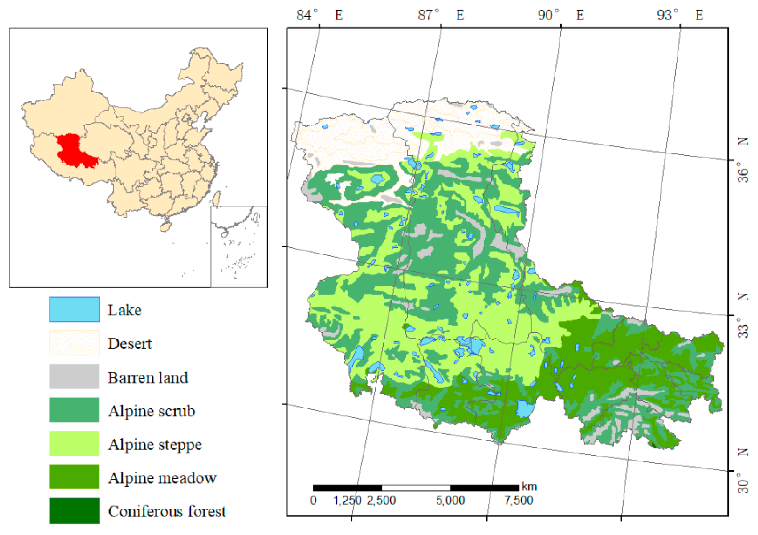
2.1. Study Area

Northern Tibet is located in the north part of the Tibetan Autonomous Region (29°55’–36°30’ N, 83°55’–95°05’ E). Northern Tibet adjoins Kunlun Mountains and Danggula Mountains to the northwest, the “Three-River Headwaters” region to the east, and Ali Plateau to the west. It covers approximately 369,000 km2, with a mean elevation of over 4500 m. Northern Tibet belongs to the typical sub-frigid zone, where the primary climatic features are dryness and coldness. The annual mean temperature ranges between –28.6 to 9.4 °C, and the annual precipitation varies from 100 mm in the northwest to 800 mm in the southeast during 2000–2015 (interpolated through meteorological station data from the China Meteorological Data Service Center (CMDC), (Figure 2). The growing season typically extends from May to September [15]. About 80% of the total precipitation occurs in this period because of atmospheric circulation and local terrain. Natural vegetation types mainly include alpine shrub, alpine steppe, and alpine meadow (Figure 1). Northern Tibet consists of 11 counties: Nagqu, Nyainrong, Amdo, Baingoin, Xainza, Nyima, Lhari, Biru, Baqen, Sog, and Shuanghu. Except for Biru and Sog, which are semi-agricultural and semi-pasture counties, the nine remaining counties are pasture areas. Animal husbandry on the grassland is the mainstay of the region’s economy. Alpine grassland, the most significant ecosystem in this area, occupies about 90% of the total area in northern Tibet and provides important subsistence for local people [37].

2.2. Datasets

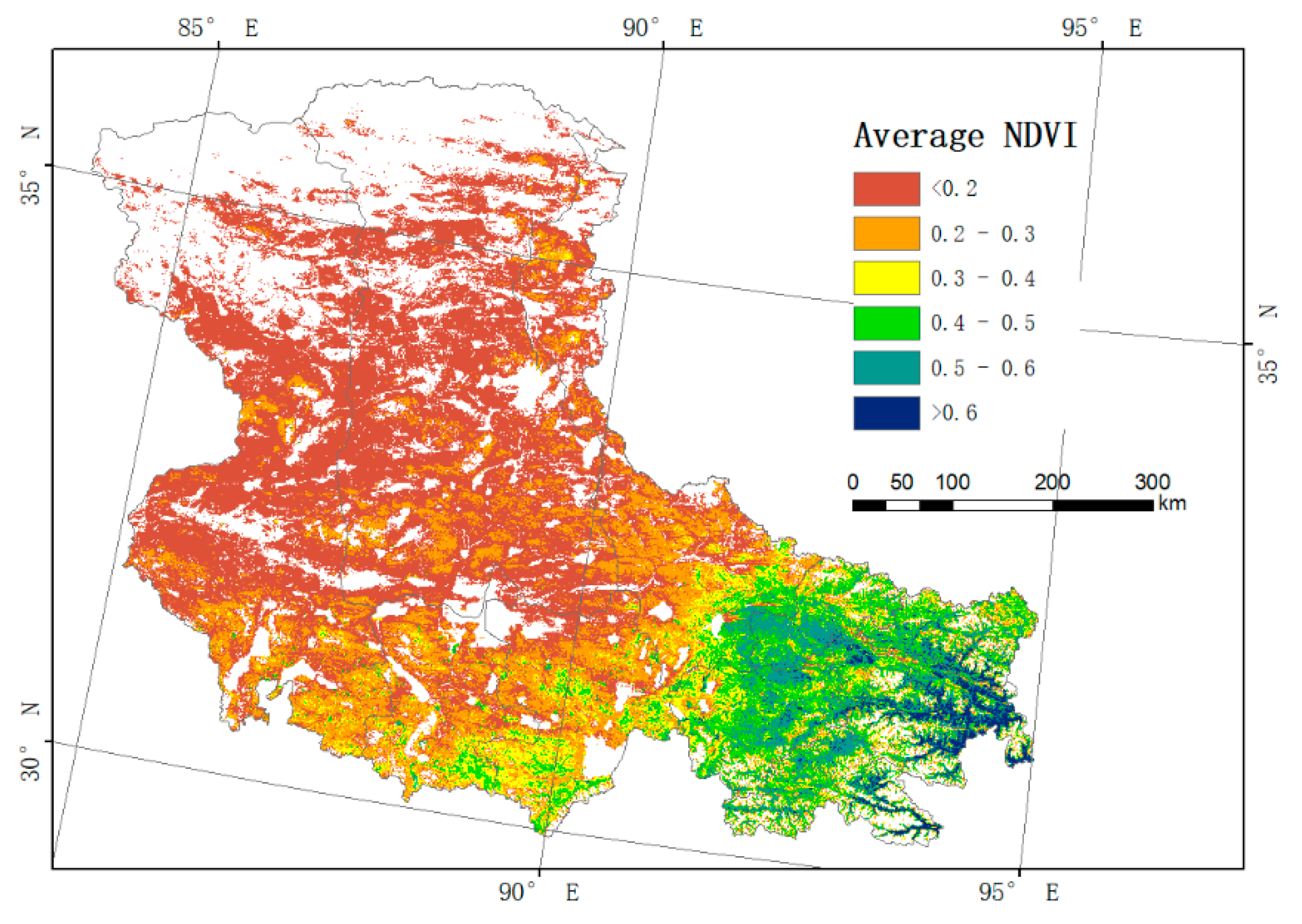
2.2.1. NDVI Time Series

The NDVI data were extracted from the terra Moderate Resolution Imaging Spectro-radiometer (MODIS) Vegetation Indices (MOD13Q1) Version 6 data, with a spatial resolution of 250 m and a temporal resolution of 16 days [38]. Four MODIS tiles, namely h24v05, h25v05, h25v06, and h26v05, were required for the study area. These MODIS tiles were mosaicked and then projected to Albers Conical Equal Area projection through MODIS Reprojection Tool (MRT) software. Then, the monthly NDVI value was calculated with the Maximum Value Composites (MVC) method, which further eliminated errors caused by cloud, atmosphere, sun angle, as well as other interference [39]. The monthly NDVI data from May to September were averaged to yield the growing season NDVI. Finally, to exclude the effects of non-vegetation factors, we extracted areas with average NDVI greater than 0.1 for further analysis [40].

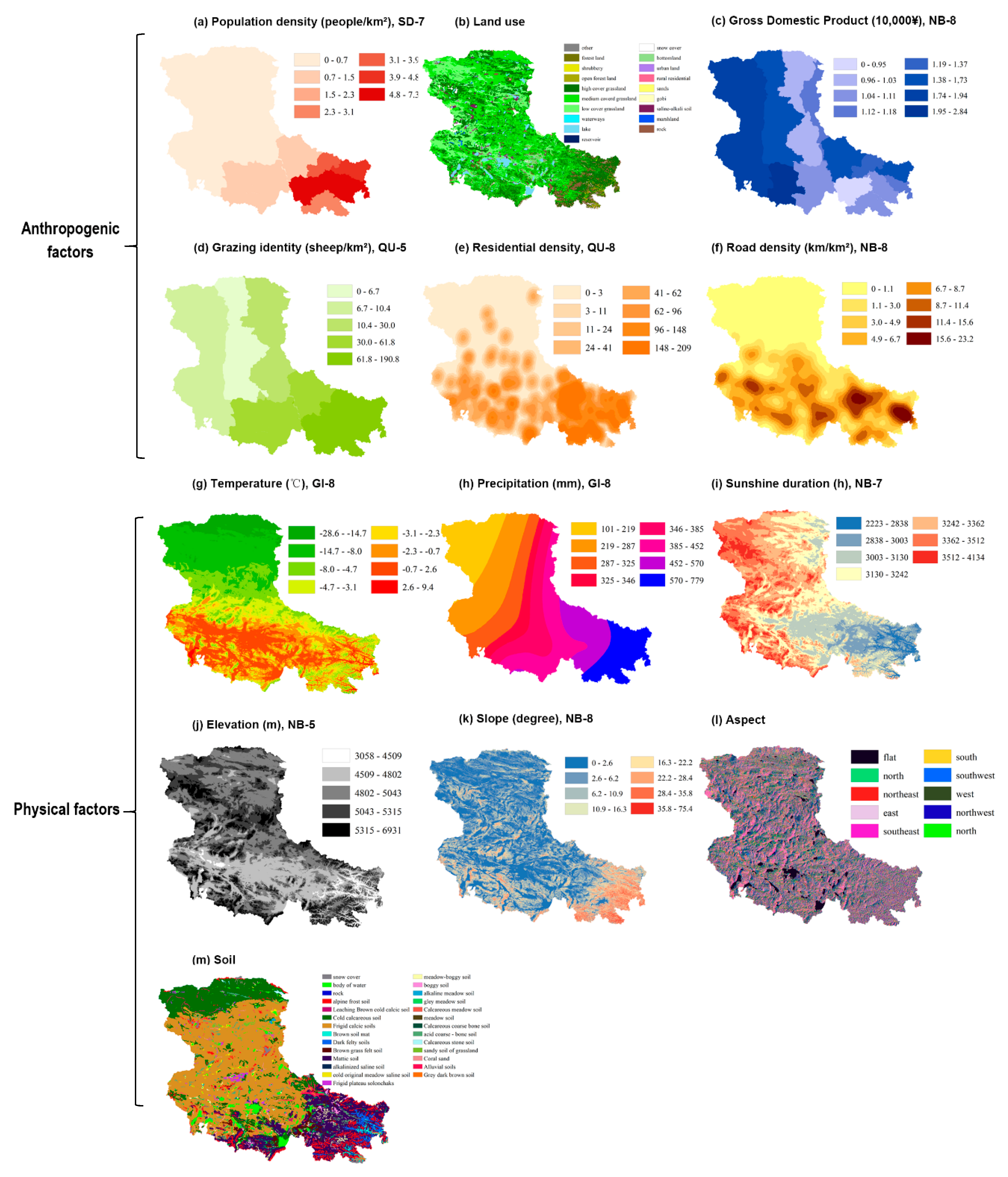
2.2.2. Physical Factors Influencing Vegetation Variation

Meteorological data, including monthly temperature, precipitation and sunshine duration datasets during the period of 2000–2015, were collected from the China Meteorological Data Service Center (CMDC). In total, original data from 39 meteorological stations were interpolated to continuous surface data with a 0.01-degree spatial resolution by using the thin-plate smoothing spline algorithm implemented in ANUSPLIN interpolation software [41].
Topographic data, including elevation, slope, and aspect, were extracted from a digital model (DEM). The DEM was obtained from Shuttle Radar Topography Mission (SRTM) terrain product data with a spatial resolution of 90 m.
Soil type data were extracted from the Soil Map of China (1:1,000,000). The dataset was based on the traditional ‘soil generation classification (CSGC)’, and provided by the Data Center for Resources and Environmental Sciences, Chinese Academy of Sciences (RESDC) (http://www.resdc.cn).
Vegetation type data were obtained from the Vegetation Map of China (1:1,000,000), and provided by the Data Center for Resources and Environmental Sciences, and the Chinese Academy of Sciences (RESDC) (http://www.resdc.cn).

2.2.3. Anthropogenic Factors Influencing Vegetation Variation

Population data, gross domestic product data, and livestock data were acquired from the official statistical surveys published in the Xizang Statistic Yearbook with a county resolution. Population density was calculated by dividing the population of each county by the area of the county. The per capita GDP was obtained by dividing the gross domestic product of the county by the corresponding population. To quantify the grazing density within each county, animal number was standardized to sheep units. Generally, a large animal, such as a horse or a yak, is equivalent to 5 sheep units, and a sheep or a goat equals 1 sheep unit [42].
Spatial Distribution Map of Land Use Types (1:1,000,000) was obtained from the land use status database in China (http://www.resdc.cn). Data production was based on Landsat TM/ETM remote sensing images as the main data source, and then generated by manual visual interpretation.
Road and resident distribution data of the study area were extracted from Open Street Map (OSM) data. With the aid of Kernel Density tool of ArcGIS software, the spatial distribution density data of road and residential areas were obtained.

2.3. Analysis

2.3.1. Mann Kendall (MK) Test

The non-parametric Mann-Kendall, proposed by Mann and Kendall [43,44], is used to detect statistically significant trends in NDVI and continuous environmental variables time series. It does not require the sample to follow a certain distribution, and the test results are basically not interfered by a few abnormal values [45]. The Mann-Kendall test statistic Z is given by:
Z = { S 1 V a r ( S ) , i f   S > 0 0 , i f   S = 0 S + 1 V a r ( S ) , i f   S < 0
S = i = 1 n 1 j = i + 1 n s g n ( x j x i )
s g n ( x j x i ) = { 1 , i f   x j x i > 0 0 , i f   x j x i = 0 1 , i f   x j x i < 0
Var ( S ) = n ( n 1 ) ( 2 n + 5 ) i = 1 m t i ( t i 1 ) ( 2 t i + 5 ) 18
where n is the length of time series, m is the number of tied groups, x i , x j and t i are the values in time series I, j (j > i) and the number of tied groups in the time series, respectively. A tied group is a set of sample data which have the same value.
The positive values of Z indicate increasing trends, while negative values show decreasing trends. The significance test is estimated by comparing Z and Z α . When – Z α < Z < Z α , the statistic Z is not statistically significant. When Z > Z α or Z < − Z α , Z is statistically significant. In this study, significant level α   = 0.05 was used. At the 5% significant level, Z α equals 1.96 correspondingly.
The sequential Mann-Kendall test is used to statistically assess the shift in trends at a regional scale and determine the beginning of a significant trend in a time series [43]. There are two series derived from the test, a progressive one U F K and a backward one, −𝐾. The calculation process of the Mann-Kendall test is as follows:
Firstly, Setting the time series as y 1 , y 2 , ... y n , m i is the cumulative number when sample y i is greater than sample y j ( 1 j i ). Define statistics:
d k = i = 1 k m i , ( 2 k n )
Then, assuming that the time series are random and independent, the mean and variance of d k are calculated as:
E ( d k ) = k ( k 1 ) 4
var ( d k ) = k ( k 1 ) ( 2 k + 5 ) 72
At last, a sequential forward series U F K value can be calculated via standardizing d k :
U F K = d k E ( d k ) v a r ( d k )
Similarly, this method is applied to calculate backward series U B K . If the value of U F K is greater than 0, the sequence shows an upward trend. If it is less than zero, it indicates a downward trend. When the value of U F K exceeds the confidence interval of ± 1.96 , it indicates a statistically significant upward or downward trend at the 95% significant level. If the intersection points of U F K and U B K curves appear within the confidence interval of ± 1.96 , it is the statistically significant trend shift point at the 95% significant level.

2.3.2. Trend Analysis

We used unary linear regression to detect the change rate of vegetation index NDVI and environment factors at each pixel, and the change rate is further input into the geographical detector model as the dependent variable. The change rate for time series x at pixel scale was calculated as
S = n × i = 1 n i × M x , i i = 1 n i × i = 1 n M x , i n × i = 1 n i 2 ( i = 1 n i ) 2
where, S is the slope of the time series x; i refers to the ordinal number 1, 2, 3, …, n corresponding to the year from 2000 to 2015; Mx,i is the mean x in the i-th year; when S > 0, the time series x shows an increasing trend, when S < 0, time series x shows a decreasing trend.

2.3.3. Geographical Detector Model

As a method to test spatial heterogeneity and to quantify the impacts of driving factors, the geographical detector model has been widely used in landscape ecological pattern, health risk assessment and the relationships between human activities and geographical conditions [35,46,47,48,49]. We assumed that the dependent variable would exhibit a similar spatial distribution, as the independent variable, if the independent variable contributes to the dependent variable [31]. Specifically, we used this model to test the consistence of spatial patterns between dependent variable y (NDVI tendency, slope of NDVI trend) and independent variable x (the factors influencing the variation of NDVI tendency), and therefore to find the essential driving forces.
The geographical detectors consist of four parts, namely factor detector, interactive detector, risk detector, and ecological detector.
The factor detector is used to quantify the contribution of impact factors. The q value implies the degree to which factor x explains the heterogeneity of y.
q H = 1 1 N * 2 i = 1 L N i * i 2
where, H represents variable y; N represents the number of total samples; and 2 represents the variance of H over the whole area. The study area is stratified into L stratums, denoted by i = 1, 2, ……, L, based on the optimal discretization methods listed below for each continuous impactor. N i represents the number in the i-th sub-region of one impact factor stratum; and i 2 represents the variance of H over the i-th sub-region of the stratum. The range of q value is 0 to 1. The larger the value of q is, the greater impact factor x makes on the heterogeneity of y. If factor x completely explains the spatial heterogeneity of y, q value equals 1; if it is totally unrelated to the spatial heterogeneity of y, q value equals 0.
The ecological detector is used to compare whether the impact of two influencing factors on the spatial distribution of vegetation tendency is significantly different or not, using the F test to measure [32]. The interactive detector, which is an advance in geographical detectors over other statistical methods, compares the q values of single factors and of interactive factors, and explores whether the two factors, when taken together, weaken or enhance one another, or have completely independent effects on a research subject. The judgment method of the interaction mode is shown in Table 1. The risk detector is used to identify vulnerable areas under potential risks in determinant strata.

2.3.4. Discretization Method

The geographical detector model is adapted to discrete factors, and can analyze continuous impact factors through appropriate discretization methods to transform the continuous data into discrete data. In this study, several impact factors, such as post-interpolation meteorological factors, elevation, slope and anthropogenic factors, are continuous variables. To avoid randomness and subjectivity of user-defined discretization, we selected the optimal discretization method from five unsupervised discretization methods, namely Equal Interval (EI), Natural Break (NB), Quantile (QU), Geometrical Interval (GI) and Standard Deviation (SD) [50]. q values are used to assess the effectiveness of different discretization methods, for which can reflect the relationships between NDVI tendency and potential driving factors, as described in 2.3.2. Here, temperature is taken as an example to explain the discretization process. First, assigning numbers of cut points. We set the number of discretion intervals as 2–8, and complete the preliminary classification of temperature based on 5 methods and 7 levels of each method. Then, extracting multi-values of the NDVI tendency layer and temperature layers of 35 discretization results. Finally, calculating and comparing the q values of temperature in each classification case. The optimal discretization method and number of intervals are determined when the q value is relatively high. The same discretization process applies to the other continuous variables. The q values of all continuous impact factors in each preliminary classification cases are shown in Appendix A. On a regional scale, the optimal discretization results of physical and anthropogenic factors’ spatial distributions are shown in Figure 2.
Statistical analyses, such as linear model, quadratic model, growth model, logarithm model, cubic model, and exponential model, were conducted to explore the linear and nonlinear relationships between main influencing factors and NDVI tendency by PASW Statistics 18.0. Regression coefficients ( b 0 , b 1 , b 2 , and b 3 ) and the goodness of fit (R2) were calculated and compared to determine which model to use.
y = b 0 + b 1 * x + b 2 * x 2 + b 3 * x 3
y = e b 0 + b 1 * x
y = b 0 + b 1 * I n ( x )
y = b 0 * e b 1 * x
R 2 = S S R S S T = 1 S S E S S T = 1 i = 1 n ( y i y i ^ ) 2 i = 1 n ( y i y ¯ ) 2
where, b 0 , b 1 , b 2 and b 3 are regression coefficients. y represents values of NDVI, x represents values of main environment factors. Each y i associated with a predicted (or modeled) value y i ^ . y ¯ is the mean value of the observed data y. SST represents the sum of the squares of the difference of the dependent variable and its mean value; SSR represents the sum of squares of regressions, which is the sum of squared deviations that reflect the degree of correlation between independent and dependent variables; SSE represents sum of squared residuals, which is a measure of the discrepancy between the data and an estimation model.

3. Results

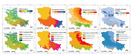
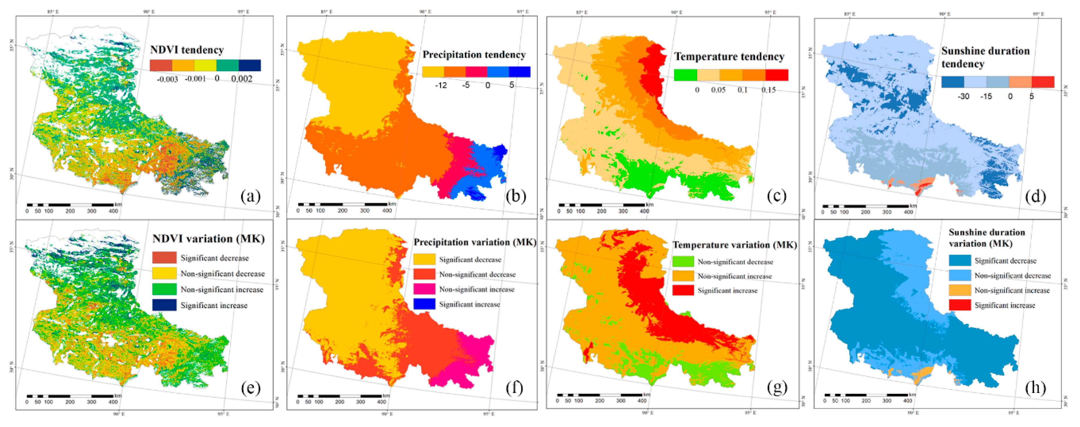
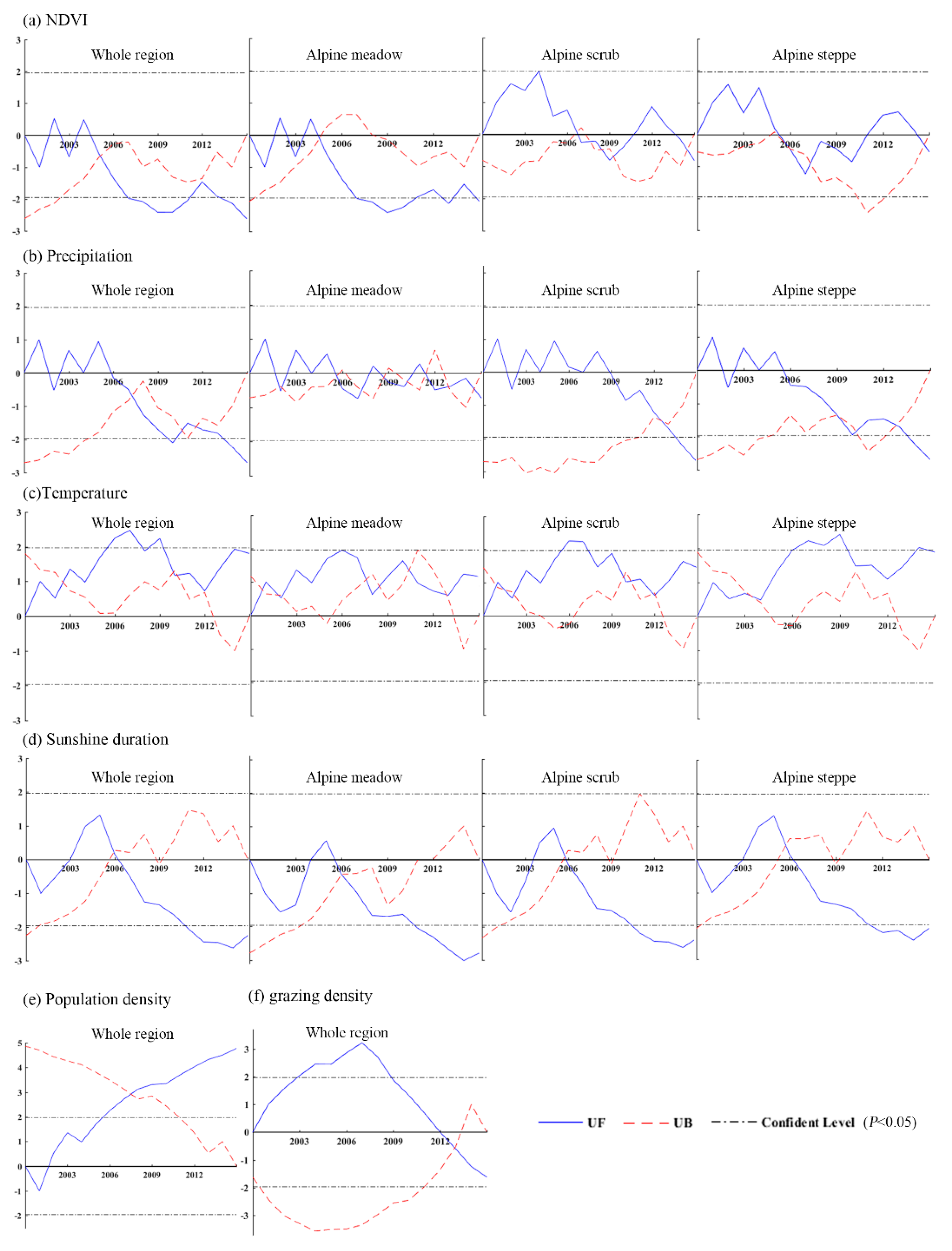
3.1. Trend and Trend Shift Analysis of NDVI and Environment Factors in Northern Tibet

From the southeast to the northwest of northern Tibet, the 16-year average NDVI had been decreasing in growing season (Figure 3). This was consistent with the regional distribution of temperature and precipitation. The northwestern counties (Nyima and Shuanghu counties) had the lowest mean NDVI value (0.16) in the whole region. For the central counties (Amdo, Shenza, and Baingoin counties) the average annual NDVI value was 0.25. In the southeastern counties (Nagqu, Nyainrong, Lhari, Biru, Sog, and Baqing counties), with an average value of 0.45 and maximum value of 0.52, the mean NDVI was higher than those of the other regions.
The spatial distribution of the slope of vegetation and environment factors trend estimated by ULR (Figure 4a–d) and corresponding significant level (P < 0.05) estimated by the MK method (Figure 4e–h) are basically consistent. Areas with recovery tendency were mainly distributed in the north and southeast part of northern Tibet, accounting for 46% (ULR method) and 49% (MK method) of alpine grassland in this region (Figure 4a,e). The southwest and central regions, which account for 54% (ULR method) and 51% (MK method) of the whole region, have already undergone a degradation tendency. In most parts of northern Tibet, the inter-annual NDVI of the alpine grassland experienced small fluctuations. Specifically, significant recovery trends mainly occurred in the north part of northern Tibet, accounting for 9% (ULR method) and 13% (MK method) of the whole area, whereas 10% (ULR method) and 11% (MK method) of the grassland showed significant degradation trends, mainly occurring in the southern part of Northern Tibet. Nagqu county (the capital of Northern Tibet, located in the south of the study area) and its surrounding areas underwent degradation or even significant degradation. Precipitation showed a decreasing trend in most parts of the study area, and declined most dramatically and significantly in the northwest (Figure 4b,f). Areas with increasing trend of precipitation were only distributed in the east part. Temperature showed an increasing trend nearly in the whole region during 2000–2015. The regions with a significant increasing trend (P < 0.05) were mainly distributed in the northeast of northern Tibet (Figure 4c,g). In most of northern Tibet, sunshine duration exhibited a significant decreasing trend (P < 0.05) (Figure 4d,h).
From 2000 to 2015, there have been decreasing trends in the average annual NDVI in the whole region and in the alpine meadow since 2004 (Figure 5a). A decreasing trend shift was found in 2005 and the trend became significant around 2007 in the whole region and in the alpine meadow (P < 0.05). Precipitation had exhibited a decreasing trend since 2006 and reached a significant level (P < 0.05) around 2013 in the whole region, in the alpine scrub and in the alpine steppe (Figure 5b). In particular, there was a decreasing trend shift around 2012 in the alpine scrub. Temperature had been increasing during the whole study period, and the increasing trend was not significant except in the period of 2005–2009 (Figure 5c). We can see that sunshine duration had exhibited a decreasing trend since 2006 in all vegetation types (Figure 5d). The U F K and U B K curves for sunshine duration intersected at 2006, and the intersected point was statistically significant, indicating that a decreasing trend shift began in 2006 and became significant around 2011. Population density across northern Tibet had exhibited an increasing trend since 2002 and became statistically significant around 2005 (P < 0.05) (Figure 5e). Grazing density in northern Tibet had increased first and then decreased since 2012 (Figure 5f).

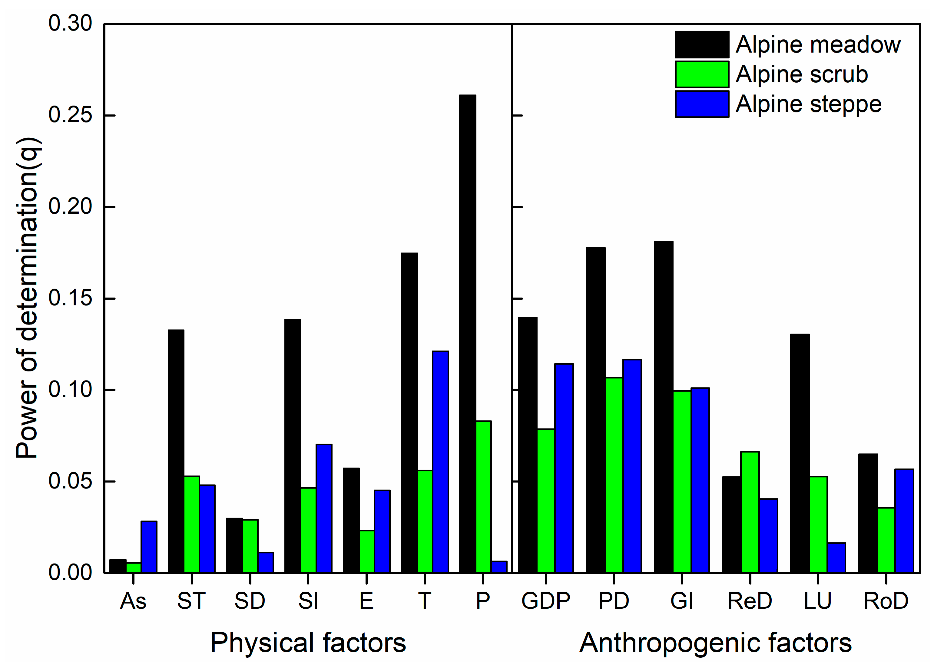
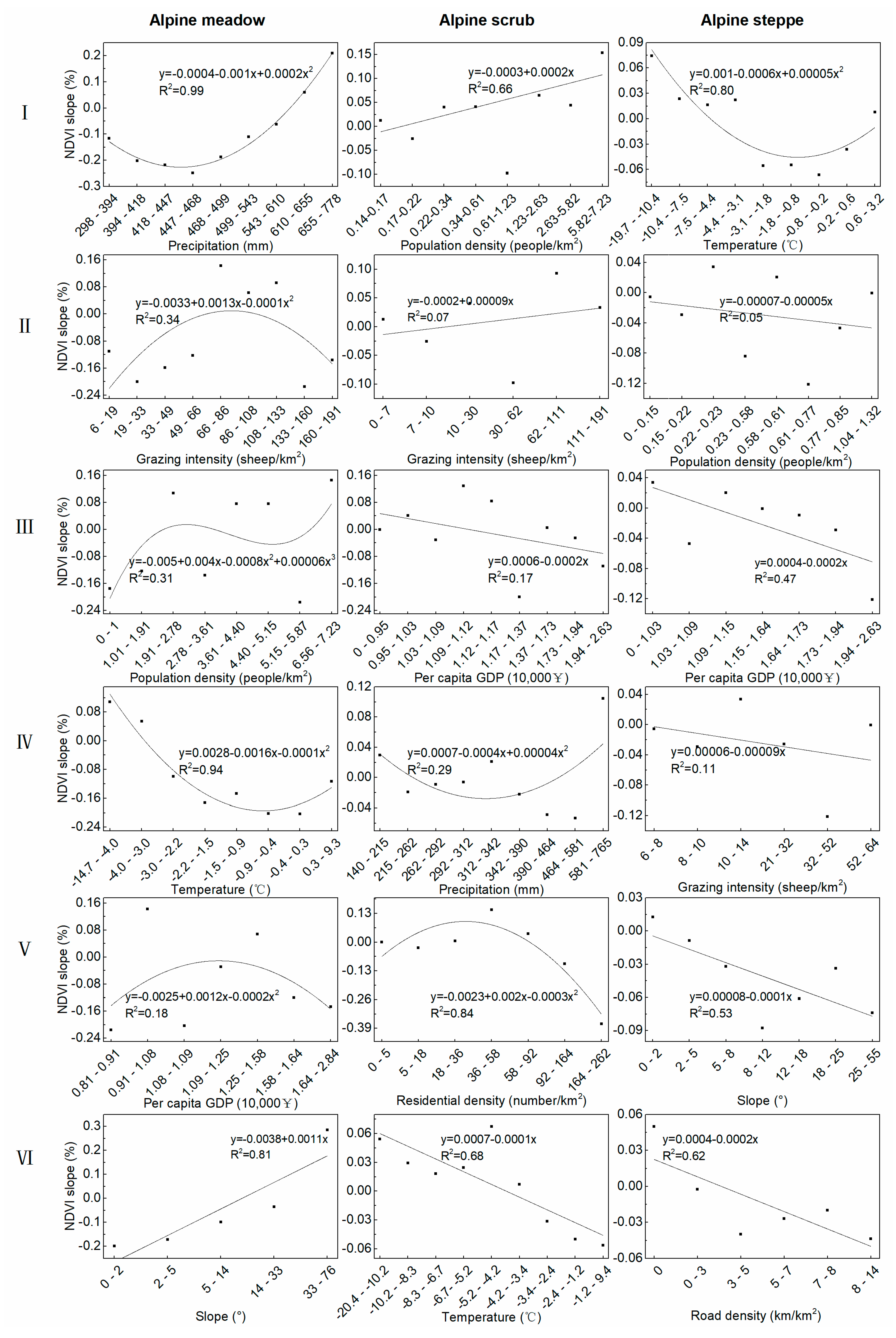
3.2. Assessing the Impact of Individual Factors on Vegetation Variation

The effects of physical and anthropogenic factors on NDVI tendency differed in three types of grassland. Moreover, the effect of the same individual factor on NDVI of various vegetation types was different (Figure 6). The q values for the alpine meadow were relatively high, which indicated that NDVI distribution was more sensitive in the alpine meadow, than in the other two types of grasslands (Table 2). The main factor that determined vegetation degradation in the alpine meadow was precipitation (0.282); in the alpine scrub, the main factor was population density (0.101); in the alpine steppe, it was temperature (0.118). Anthropogenic factors, such as population density, grazing density and per capita GDP, influenced all vegetation types hugely. q values and order of them were very close. In the alpine meadow, grazing density (0.205) and population density (0.201) ranked second and third, respectively. In the alpine scrub areas, population density (0.101), grazing density (0.096) and per capita GDP (0.087) ranked top three. In the alpine steppe, population density (0.115), per capita GDP (0.112) and grazing density (0.101) ranked second, third and fourth, respectively.
Most of the physical factors and the tendency of NDVI had better simulation results, with larger r square, compared with anthropogenic factors in the three vegetation types (Figure 7). The most serious vegetation degradation appeared in the areas with fewer rainfalls in the alpine meadow, showing that the tendency of NDVI decreased first and then increased on the spatial scale with the increase of precipitation. In terms of temperature, the most serious vegetation degradation appeared in the areas with higher temperature for the whole region, showing that the tendency of NDVI decreased first and then increased with the increase of temperature in regions of the alpine meadow and the alpine steppe. By contrast, NDVI tendency was significantly negatively correlated with temperature in the alpine scrub (slope = –0.00013, P < 0.01). It is worth noting that terrain slope displayed a significantly positive correlation with NDVI tendency in the alpine meadow (slope = 0.0011, P < 0.05), while in the alpine steppe, terrain slope showed a marginally significantly negative correlation (slope = –0.0001, P = 0.06). In terms of anthropogenic factors, residential density in the alpine scrub, per capita GDP and road density in the alpine steppe, it showed that, generally, the higher each density was, the more serious the vegetation degradation was. However, the alpine scrub presented the opposite result: the smaller the population density was, the more serious the vegetation degradation was.

3.3. Interaction between Factors That Influence Vegetation Variation

All interactive q values, divided into two categories: double factor enhancement and nonlinear enhancement, were greater than the highest q value of any of their individual factors. This indicates that the interaction between factors played an essential role in vegetation variation. In the alpine meadow, the interaction of precipitation with other physical factors was the most significant (Table 3). Particularly, the interaction between precipitation and temperature can explain 44.6% of the vegetation variation in the alpine meadow. In the alpine scrub, the interaction between temperature and GDP was the highest, which accounted for a 27.5% change of vegetation variation. For the alpine steppe, the top three interactions were the soil type associated with other influencing factors. For example, the interaction between soil and population can explain a 29.4% change of the vegetation variation. In these three vegetation types, the interaction effects of the main factors were greater in the alpine meadow than those in the other two vegetation types.

3.4. Identification of Areas Vulnerable to Vegetation Degradation

The spatial distribution of each vegetation type that is vulnerable to vegetation degradation was significantly different (Figure 8). In the alpine meadow, the risk of vegetation degradation reached the maximum in areas where annual average precipitation levels were between 448 to 469 mm. However, in the alpine scrub, the highest risk of vegetation degradation was observed in the regions with annual average population density between 0.61–1.23 people/km2, and in the alpine steppe, it was the areas with annual average temperatures between –0.83 to –0.15 °C.

4. Discussion

The results show that NDVI decreased from 2000 to 2015 across northern Tibet. Previous studies have shown that NDVI tendency varied with the different spatio-temporal scale on the Tibet plateau [10,51]. The inconsistency of NDVI change rate may result from the spatially heterogeneous of climate, land use policies as well as the uncertainty of remote sensing data. The state of climate factors, such as temperature, precipitation and solar radiation varied in ecosystem zones, where the vegetation composition and humidity differed. The state has implemented a pilot project of “returning grazing to grassland” in Tibet since 2004, whose layout and implementation differed on a regional scale. For example, research has shown that the response degree to this “returning grazing to grassland” project in the alpine meadow was obviously higher than that in the alpine grassland [52]. Additionally, both the scale effect and the uncertainty influence the accuracy of the data, causing the inconsistency results of NDVI tendency in studies. Vegetation parameters, such as NDVI, leaf area index (LAI) [53,54], are needed for validation in future studies. The multi-annual average NDVI from our studies shows the same spatial distribution as previous research with a declining trend from the southeast to the northwest of northern Tibet [55], which is consistent with the water and heat distribution pattern in geographic space. Nagqu county and its surrounding areas are well supplied with a good condition of water resource and temperature. However, these areas have been undergoing significant degradation due to the fast society and economy development. Different grassland types’ responses to environment factors differed. NDVI variation in the alpine meadow was generally more sensitive to influencing factors than that in the alpine steppe. This result was similar with the previous studies [16,56]. The alpine steppe in the Tibet plateau is cold-resistant and drought-tolerant, where perennial dense clumps, rhizomes, and shrubs are dominating vegetation. By contrast, the alpine meadow has a relatively simple plant community composition dominated only by perennial herbaceous species. Also, the alpine meadow has high population density; therefore, it is more vulnerable to environmental changes [57].
The dominant driving factors of vegetation variation differed in each vegetation type of northern Tibet, primarily because the areas with diverse vegetation types can present different environmental conditions, and also because the vegetation with specific physiological characteristics has different interactions with environmental factors. Specifically, precipitation was the key factor that influenced the alpine meadow variation, whereas temperature was the key factor that contributed to the alpine steppe variation. Previous studies have yielded different results on the factors’ effects on vegetation variation. For example, Sun and Ding suggested that mean annual precipitation had the greatest effect on the alpine meadow [16,56,58]. Shen et al. found that no significant correlation had been found between the maximum vegetation index and temperature or precipitation in the growing season across the Tibetan Plateau [19]. Obviously, there are still some controversies about the driving factors of different vegetation types. Therefore, further research is needed to explore the relationships between meteorological factors and different vegetation types. Statistical analysis showed that the areas under higher temperature and lower precipitation had higher risk of vegetation degradation. This result agrees well with the findings of Zhang and Cui [55,59]. Increased temperatures and reduced precipitation will worsen atmospheric drought and decrease relative humidity. Hence, this causes a climate drought, which is not conducive to the improvement and maintenance of the grassland ecosystem productivity in the region. The statistical analysis between NDVI tendency and terrain slope indicates that the flatter the terrain in the alpine meadow is, and the steeper the area in the alpine steppe is—the greater the level of vegetation degradation is. These two opposite results may be attributed to the effects of terrain slope on water use efficiency. Where the slope of the alpine steppe is steep, the soil moisture content is low and is not conducive to the growth of vegetation, and the vegetation degradation there is more serious. For the alpine meadow, water is not a limiting factor for plant growth [57]. Instead, human activities are intensive in flat areas. Therefore, vegetation degradation is more serious there.
The anthropogenic factors, such as population density, grazing density and per capita GDP, influenced the alpine scrub variation greatly. Particularly, these factors influenced the alpine meadow and the alpine steppe hugely. The higher the residential density in the alpine scrub is, or the higher per capita GDP or road density in the alpine steppe is, the more serious the vegetation degradation is. This result is parallel with a previous study showing that the degradation of vegetation areas closer to the highway was more severe [30]. We also found that the q values and the order of population density, grazing density and per capita GDP are very close, although the method we used excluded the influence of multiple collinearity among the factors. It indicated that the relationships between the anthropogenic factors are closer than those between the physical factors. Actually, the interference of the anthropogenic factors in the Tibet plateau is not as complicated as that in other livable and developed places. Grazing is the primary factor affecting the ecological environment on the plateau [5,6,8]. Where there are a large number of livestock units, there is often large population density and high social productivity. Therefore, the synthetic influence index of the anthropogenic factors can be considered to simplify the study of quantifying effects of the anthropogenic activities.
The complexity of the geographical processes suggests that multiple factors of environment interactively affect vegetation degradation or recovery. The results of the interactive detector show that the interaction between factors can greatly enhance the explanatory power of vegetation variation. Precipitation was the most significant factor that affected the alpine meadow variation, and it also played an important role in the interaction of factors. These results highlight the importance of precipitation in the alpine meadow. Our results denote that precipitation shows a decreasing trend, temperature shows an increasing trend, and sunshine duration shows a significant decreasing trend on both the temporal and spatial scales (Figure 4b–d), (Figure 5b–d). Previous research has shown that precipitation is positively correlated with vegetation growth on a global scale [60]. The interaction between temperature and precipitation enlarges the impact on vegetation variation because of the decrease of precipitation and the acceleration of evapotranspiration by the increase of temperature, which results in water stress. Altitude is directly related to temperature, precipitation, soil organic matter and vegetation coverage [61,62], and when the effect of precipitation is superimposed with altitude, it has a greater impact on vegetation. Sunshine duration can be used to estimate photosynthetically active radiation (PAR) [63]. PAR refers to the solar spectral components that can be photosynthesized by green plants. It mainly affects the growth and development of plants by controlling photosynthesis [64]. Therefore, the decrease of sunshine duration will aggravate the adverse effects on vegetation caused by the decrease of precipitation. The explanatory power of soil on the alpine steppe variation was greatly enhanced by the interaction with the anthropogenic factors. The alpine steppe has small vegetation coverage, thus has low soil and water conservation function. On the other hand, the physical and chemical properties of soil are easily affected by human activities, so the combination of human activities and soil factors has a greater impact on vegetation.
Considering the results of factor detector and interactive detector, we conclude that the physical factors, rather than the anthropogenic factors have been the primary driving factors for vegetation dynamics across northern Tibet during 2000 and 2015. This result consists with the previous findings conducted in the similar ecosystems [10,42]. The anthropogenic factors, especially population density and grazing density, also play important roles in vegetation variation. In our study, precipitation, temperature, and sunshine duration are the dominant physical factors influencing vegetation variation. Especially, the decreasing trend of precipitation, increasing trend of temperature, and decreasing trend that sunshine duration may cause an unsuitable environment for vegetation growth. In this case, we indicate that the effects of the anthropogenic factors may be magnified when climate conditions become unfavorable for vegetation. As we all know, the ecosystem in the Qinghai-Tibet plateau are vulnerable and extremely sensitive to the changing environment. We can not regulate climate in the short term, but corresponding measures and adaptive strategies should be taken to regulate the negative impacts of human activities, and ultimately to achieve sustainable development of the alpine ecosystems.

5. Conclusions

In summary, based on the NDVI time series, this study explored the issue of vegetation variation on the alpine grassland ecosystem. Our study clearly showed a significant decreasing trend of vegetation index across northern Tibet during the period of 2000–2015. The physical factors, rather than the anthropogenic factors, have been the primary driving factors for vegetation dynamics, while the effects of the anthropogenic factors may be magnified when the physical environment is unsuitable for vegetation growth. Specifically, meteorological factors were the primary factors that determined vegetation variation in the alpine meadow and the alpine scrub, and the anthropogenic factors influenced the alpine scrub variation the most. The interactions between the driving factors had a larger effect on vegetation than any single factor. In the alpine meadow, the areas with high altitude may improve the impact of precipitation on vegetation. Meanwhile, decreasing precipitation combined with increasing temperature and decreasing sunshine duration may potentially enhance the degradation of the grasslands, while the soil types and the anthropogenic factors together have resulted in a reduction of grassland plant cover in the alpine steppe. In addition, the influence of population density is highly similar to that of grazing density, which may provide access to simplify the study of the anthropogenic activities in the plateau ecosystem. Although this study integrally quantified the influence of environment factors on vegetation variation, it failed to identity the dominant factors at a sub-region scale. Finer resolution data are needed for further studies.

Author Contributions

Conceptualization, Q.R. and Y.H.; Methodology, Q.R.; Software, X.S.; Validation, X.C. and K.X.; Formal analysis, Q.R.; Investigation, C.X. and B.D.; Data curation, Q.R.; Writing—original draft preparation, Q.R.; Writing—review and editing, Y.H., A.X., W.L. and R.H.; Visualization, Q.R.; Supervision, Y.W.

Funding

This research was funded by the following projects: the CAS Strategic Priority Research Programme (Grant No. XDA20050103 and XDA19030202), International Cooperation and Exchange of National Natural Science Foundation of China (Grant No. 31761123001, 31761143018), and Science and Technology Service Network Initiative (kfj-sts-zdtp-013).

Acknowledgments

We thank Yu Hua for her language assistance during the preparation of this manuscript. Great thanks for the help of Inner Mongolia Grassland Ecosystem Research Station, CAS.

Conflicts of Interest

The authors declare no conflict of interest.

Appendix A

Geographical detector model is adapted to discrete factors, and can analyze the continuous impact factors through appropriate discretization methods to transform the continuous data into discrete data. Table A1 presents the q values of continuous impact factors in each preliminary classification cases. The optimal discretization method and number of intervals are determined when the q values are relatively high. The categorization method, EI, NB, QU, GI and SD stand for the discretization methods of Equal Interval, Natural Break, Quantile, Geometrical Interval and Standard Deviation, respectively. The number 2–8 means the discretion intervals of each method. On a regional scale, the optimal discretization results of physical and anthropogenic factors’ spatial distributions are shown in Figure 2.
Table A1. The q values of continuous impact factors in each preliminary classification cases.
Discretization MethodsFactorsq Values
2345678
EITemperature0.0585 0.1400 0.0612 0.1753 0.1677 0.1418 0.1677
NB0.1245 0.1663 0.1550 0.1632 0.1826 0.1849 0.1831
QU0.1562 0.1448 0.1649 0.1833 0.1782 0.1839 0.1867
GI0.1625 0.1559 0.1382 0.1247 0.1900 0.1729 0.2019
SD----0.1705 --
EIPrecipitation0.4816 0.4600 0.5277 0.5097 0.5578 0.5447 0.5608
NB0.4752 0.4650 0.5260 0.5564 0.5528 0.5655 0.5580
QU0.2805 0.4363 0.5134 0.5261 0.5324 0.5478 0.5678
GI0.3053 0.4606 0.4853 0.5333 0.5403 0.5460 0.5680
SD----0.5498 --
EIElevation0.0494 0.0686 0.0618 0.1038 0.1078 0.1118 0.1634
NB0.0486 0.0865 0.0957 0.1791 0.1569 0.1582 0.1485
QU0.0501 0.0756 0.0891 0.0983 0.1015 0.1106 0.1082
GI0.0494 0.0657 0.0886 0.0867 0.0989 0.1382 0.1276
SD----0.1594 --
EISlope0.0048 0.0676 0.0750 0.0990 0.0989 0.1092 0.1146
NB0.0795 0.1017 0.1067 0.1189 0.1226 0.1161 0.1231
QU0.0494 0.0709 0.0931 0.0942 0.1063 0.1095 0.1089
GI0.0493 0.0884 0.0982 0.1160 0.1042 0.1067 0.1107
SD--0.1100 ---0.1193
EIRoads density0.1471 0.1407 0.1904 0.2186 0.2305 0.2427 0.2500
NB0.1186 0.1943 0.2575 0.2566 0.2672 0.2733 0.2781
QU0.1294 0.1603 0.1676 0.1856 0.1975 0.2164 0.2252
GI0.1414 0.1707 0.1777 0.2706 0.2682 0.2679 0.2737
SD--0.2345 ---0.2758
EIResidential density0.0404 0.0633 0.0768 0.1198 0.1493 0.1929 0.2380
NB0.0698 0.3401 0.3736 0.3795 0.4296 0.4405 0.4346
QU0.1962 0.3357 0.4026 0.4438 0.4484 0.4393 0.4568
GI0.1884 0.3412 0.3828 0.3820 0.4411 0.4470 0.4377
SD--0.3215 -- 0.4441
EISunshine duration0.2508 0.2373 0.2842 0.3910 0.3861 0.4229 0.4365
NB0.1922 0.3571 0.4385 0.4607 0.4657 0.4956 0.4790
QU0.1651 0.2925 0.3651 0.3835 0.4212 0.4314 0.4722
GI0.1293 0.3707 0.4204 0.4304 0.4575 0.4478 0.4821
SD---- 0.4677
EIGrazing density0.3368 0.4621 0.5313 0.5626 0.5670 0.5810 0.6085
NB0.4587 0.5092 0.5825 0.6069 0.6075 0.6077 0.6089
QU0.3836 0.5174 0.5187 0.6412 0.5898 0.6281 0.6278
GI0.3836 0.4583 0.5448 0.5944 0.5952 0.5559 0.5949
SD---0.5770 -0.6088 -
EIPopulation density0.3309 0.4300 0.5448 0.5445 0.5454 0.5449 0.5779
NB0.4274 0.5409 0.5414 0.6194 0.6218 0.6227 0.6227
QU0.3753 0.5022 0.5030 0.6349 0.5767 0.6296 0.6332
GI0.2217 0.3758 0.5293 0.5297 0.6210 0.6327 0.6327
SD--0.6163 --0.6356 -
EIPer Capita GDP0.1170 0.1683 0.1237 0.1392 0.2074 0.2587 0.2009
NB0.1170 0.1693 0.1760 0.2074 0.3520 0.3527 0.3884
QU0.0900 0.0649 0.0902 0.2068 0.2900 0.3047 0.3548
GI0.1827 0.1219 0.1441 0.1837 0.2009 0.1613 0.2725
SD-----0.1486 -
Figure A1 shows the inter-annual change of population density and grazing density over the northern Tibet during 2000–2015. The population density is generally small, and the county with the highest population density (Sog county) is less than 10 people per square kilometer. Population density increases slowly with years. The counties with small grazing density, such as Nyima, Xainza, Amdo, Baingoin and Lhari changes slowly with years. However, counties with large grazing density, such as Nagqu, Nyainrong and Baqen, shows the trend of increasing first and then decreasing. There were large differences between counties of both population density and grazing density. The grazing density and population density are higher in counties in the southern and eastern area, which underwent relatively rapid social and ecological development.
Figure A1. The trends of (a) Population density and (b) Grazing density at county scale.
Remotesensing 11 01183 g0a1

References

  1. Zavaleta, E.S.; Shaw, M.R.; Chiariello, N.R.; Mooney, H.A.; Field, C.B. Additive effects of simulated climate changes, elevated CO2, and nitrogen deposition on grassland diversity. Proc. Natl. Acad. Sci. USA 2003, 100, 7650–7654. [Google Scholar] [CrossRef]
  2. Xu, X.K.; Hong, C.; Levy, J.K. Spatiotemporal vegetation cover variations in the Qinghai-Tibet Plateau under global climate change. Chin. Sci. Bull. 2008, 53, 915–922. [Google Scholar] [CrossRef]
  3. Chengqun, Y.; Zhang, Y.; Claus, H.; Zeng, R.; Zhang, X.; Wang, J. Ecological and environmental issues faced by a developing Tibet. Environ. Sci. Technol. 2012, 46, 1979. [Google Scholar]
  4. Leroux, L.; Béguéb, A.; Lo Seen, D.; Jolivotb, A.; Kayitakirec, F. Driving forces of recent vegetation changes in the Sahel: Lessons learned from regional and local level analyses. Remote Sens. Environ. 2017, 191, 38–54. [Google Scholar] [CrossRef]
  5. Gao, Q.Z.; Wan, Y.F.; Li, Y.; Qin, X.B.; Jiangcun, W.; Xu, X.M. Spatial and temporal pattern of alpine grassland condition and its response to human activities in Northern Tibet, China. Rangel. J. 2010, 32, 165–173. [Google Scholar] [CrossRef]
  6. Nan, Z. The grassland farming system and sustainable agricultural development in China. Grassl. Sci. 2005, 51, 15–19. [Google Scholar] [CrossRef]
  7. Harris, R.B. Rangeland degradation on the Qinghai-Tibetan plateau: A review of the evidence of its magnitude and causes. J. Arid Environ. 2010, 74, 1–12. [Google Scholar] [CrossRef]
  8. Li, X.L.; Gao, J.; Brierley, G.; Qiao, Y.-M.; Zhang, J.; Yang, Y.-W. Rangeland degradation on the Qinghai-Tibet Plateau: Implications for rehabilitation. Land Degrad. Dev. 2013, 24, 72–80. [Google Scholar] [CrossRef]
  9. Wang, Z.Q.; Zhang, Y.; Yang, Y.; Zhou, W.; Gang, C.; Zhang, Y.; Li, J.; An, R.; Wang, K.; Odeh, I.; et al. Quantitative assess the driving forces on the grassland degradation in the Qinghai-Tibet Plateau, in China. Ecol. Inform. 2016, 33, 32–44. [Google Scholar] [CrossRef]
  10. Huang, K.; Zhang, Y.; Zhu, J.; Liu, Y.; Zu, J.; Zhang, J. The influences of climate change and human activities on vegetation dynamics in the Qinghai-Tibet Plateau. Remote Sens. 2016, 8, 876. [Google Scholar] [CrossRef]
  11. Ji, L.; Peters, A.J. Lag and Seasonality Considerations in Evaluating AVHRR NDVI Response to Precipitation. Photogramm. Eng. Remote Sens. 2005, 71, 1053–1061. [Google Scholar] [CrossRef]
  12. Schultz, P.A.; Halpert, M.S. Global correlation of temperature, NDVI and precipitation. Adv. Space Res. 1993, 13, 277–280. [Google Scholar] [CrossRef]
  13. Gómez-Mendoza, L.; Galicia, L.; Cuevas-Fernández, M.L.; Magaña, V.; Gómez, G.; Palacio-Prieto, J.L. Assessing onset and length of greening period in six vegetation types in Oaxaca, Mexico, using NDVI-precipitation relationships. Int. J. Biometeorol. 2008, 52, 511–520. [Google Scholar] [CrossRef] [PubMed]
  14. Xia, Z.; Hu, H.; Shen, H.; Zhou, D.; Zhou, L.; Myneni, R.B.; Fang, J. Satellite-indicated long-term vegetation changes and their drivers on the Mongolian Plateau. Landsc. Ecol. 2015, 30, 1599–1611. [Google Scholar]
  15. Shen, M.; Piao, S.; Jeong, S.-J.; Zhou, L.; Zeng, Z.; Ciais, P.; Chen, D.; Huang, M.; Jin, C.-S.; Li, L.Z.X.; et al. Evaporative cooling over the Tibetan Plateau induced by vegetation growth. Proc. Natl. Acad. Sci. USA 2015, 112, 9299–9304. [Google Scholar] [CrossRef] [PubMed] [Green Version]
  16. Jian, S.; Qin, X.; Yang, J. The response of vegetation dynamics of the different alpine grassland types to temperature and precipitation on the Tibetan Plateau. Environ. Monit. Assess. 2016, 188, 1–11. [Google Scholar]
  17. Sun, J.; Cheng, G.; Li, W.; Sha, Y.; Yang, Y. On the variation of NDVI with the principal climatic elements in the Tibetan Plateau. Remote Sens. 2013, 5, 1894–1911. [Google Scholar] [CrossRef]
  18. Chu, D.; Lu, L.; Zhang, T. Sensitivity of normalized difference vegetation index (NDVI) to seasonal and interannual climate conditions in the Lhasa area, Tibetan Plateau, China. Arct. Antarct. Alp. Res. 2007, 39, 635–641. [Google Scholar] [CrossRef]
  19. Shen, Z.; Fu, G.; Yu, C.; Sun, W.; Zhang, X. Relationship between the growing season maximum enhanced vegetation index and climatic factors on the Tibetan Plateau. Remote Sens. 2014, 6, 6765–6789. [Google Scholar] [CrossRef]
  20. Dardel, C.; Kergoat, L.; Hiernaux, P.; Mougin, E.; Grippa, M.; Tucker, C.J. Re-greening Sahel: 30 years of remote sensing data and field observations (Mali, Niger). Remote Sens. Environ. 2014, 140, 350–364. [Google Scholar] [CrossRef]
  21. Piao, S.; Fang, J.; He, J. Variations in vegetation net primary production in the Qinghai-Xizang Plateau, China, from 1982 to 1999. Clim. Change 2006, 74, 253–267. [Google Scholar] [CrossRef]
  22. Gao, Q.; Li, Y.; Wan, Y.; Qin, X.; Jiangcun, W.; Liu, Y. Dynamics of alpine grassland NPP and its response to climate change in Northern Tibet. Clim. Chang. 2009, 97, 515. [Google Scholar] [CrossRef]
  23. Liu, L.; Yili, Z.; Wanqi, B.; Jianzhong, Y.; Mingjun, D.; Zhenxi, S.; Shuangcheng, L.; Du, Z. Characteristics of grassland degradation and driving forces in the source region of the Yellow River from 1985 to 2000. J. Geogr. Sci. 2006, 16, 131–142. [Google Scholar] [CrossRef]
  24. Fassnacht, F.E.; Li, L.; Fritz, A. Mapping degraded grassland on the Eastern Tibetan Plateau with multi-temporal Landsat 8 data—Where do the severely degraded areas occur? Int. J. Appl. Earth Obs. Geoinf. 2015, 42, 115–127. [Google Scholar] [CrossRef]
  25. Zhang, Y.; Liu, L.; Yili, Z.; Wanqi, B.; Jianzhong, Y.; Mingjun, D.; Zhenxi, S.; Shuangcheng, L.; Du, Z. Grassland degradation in the source region of the Yellow River. Acta Geogr. Sin. 2006, 61, 3–14. [Google Scholar]
  26. Hui, Z.; Ning, K.N.; Shu Juan, L.I. Human impacts on landscape structure in Wolong Natural Reserve. Acta Ecol. Sin. 2001, 21, 1994–2001. [Google Scholar]
  27. Evans, J.; Geerken, R. Discrimination between climate and human-induced dryland degradation. J. Arid Environ. 2004, 57, 535–554. [Google Scholar] [CrossRef]
  28. Fang, X.; Zhu, Q.; Chen, H.; Ma, Z.; Wang, W.; Song, X.; Zhao, P.; Peng, C. Analysis of vegetation dynamics and climatic variability impacts on greenness across Canada using remotely sensed data from 2000 to 2009. J. Appl. Remote Sens. 2014, 8, 243–247. [Google Scholar] [CrossRef]
  29. Zhou, X.Y.; Shi, H.D.; Wang, X.R. Impact of climate change and human activities on vegetation coverage in the Mongolian Plateau. Arid Zone Res. 2014, 31, 604–610. [Google Scholar]
  30. Song, C.Q.; SongCai, Y.; GaoHuan, L.; LingHong, K.; XinKe, Z. Spatio-temporal pattern and change of Nagqu grassland and the influence of human factors. Acta Prat. Sin. 2012, 21, 1–10. [Google Scholar]
  31. Wang, J.F.; Li, X.-H.; Christakos, G.; Liao, Y.-L.; Zhang, T.; Gu, X.; Zheng, X.-Y. Geographical detectors-based health risk assessment and its application in the neural tube defects study of the Heshun region, China. Int. J. Geogr. Inf. Sci. 2010, 24, 107–127. [Google Scholar] [CrossRef]
  32. Wang, J.; Xu, C. Geodetector: Principle and prospective. Acta Geogr. Sin. 2017, 72, 116–134. [Google Scholar]
  33. Liang, P.; Yang, X. Landscape spatial patterns in the Maowusu (Mu Us) Sandy Land, northern China and their impact factors. CATENA 2016, 145, 321–333. [Google Scholar] [CrossRef]
  34. Du, Z.; Xu, X.; Zhang, H.; Wu, Z.; Liu, Y. Geographical detector-based identification of the impact of major determinants on aeolian desertification risk. PLoS ONE 2016, 11, e0151331. [Google Scholar] [CrossRef] [PubMed]
  35. Wang, J.F.; Hu, Y. Environmental health risk detection with GeogDetector. Environ. Model. Softw. 2005, 33, 114–115. [Google Scholar] [CrossRef]
  36. Liu, S.Z.; Zhou, L.; Qiu, C.S.; Zhang, J.P.; Fang, Y.P.; Gao, W.S. Studies on Grassland Degradation and Desertification of Naqu Prefecture in Tibet Autonomous Region; The Tibet People’s Publishing House: Lhasa, China, 1999. [Google Scholar]
  37. Zhang, X.; Lu, X.; Wang, X. Spatial-temporal NDVI variation of different alpine grassland classes and groups in Northern Tibet from 2000 to 2013. Mt. Res. Dev. 2015, 35, 254–263. [Google Scholar] [CrossRef]
  38. Didan, K. MOD13Q1 MODIS/Terra Vegetation Indices 16-Day L3 Global 250m SIN Grid V006 [Data set]; NASA EOSDIS LP DAAC: Sioux Falls, SD, USA, 2015. [Google Scholar]
  39. Stow, D.; Hope, P.A.; Engstrom, R.; Coulter, L. Greenness trends of Arctic tundra vegetation in the 1990s: comparison of two NDVI data sets from NOAA AVHRR systems. Int. J. Remote Sens. 2007, 28, 4807–4822. [Google Scholar] [CrossRef]
  40. Yang, Y.H.; Shi-Long, P. Variations in grassland vegetation cover in relation to climatic factors on the Tibetan Plateau. J. Plant Ecol. 2006, 30, 1–8. [Google Scholar]
  41. Hutchinson, M.F. Interpolating mean rainfall using thin plate smoothing splines. Int. J. Geogr. Inf. Syst. 1995, 9, 385–403. [Google Scholar] [CrossRef] [Green Version]
  42. Lehnert, L.W.; Wesche, K.; Trachte, K.; Reudenbach, C.; Bendix, J. Climate variability rather than overstocking causes recent large scale cover changes of Tibetan pastures. Sci. Rep. 2016, 6, 24367. [Google Scholar] [CrossRef] [Green Version]
  43. Sneyers, R. On the Statistical Analysis of Series of Observations; World Meteorological Organization: Geneva, Switzerland, 1990. [Google Scholar]
  44. Sneyers, R. Sur la Determination de la Stabilite des Series Climatologiques. In Changes of Climate: Proceedings of the Rome Symposium/Organized by Unesco and the World Meteorological Organization; Unesco: Paris, France, 1963. [Google Scholar]
  45. Sayemuzzaman, M.; Jha, M. Seasonal and annual precipitation time series trend analysis in North Carolina, United States. Atmos. Res. 2014, 137, 183–194. [Google Scholar] [CrossRef]
  46. Chen, Z.; Chen, D.; Xie, X.; Cai, J.; Zhuang, Y.; Cheng, N.; He, B.; Gao, B. Spatial self-aggregation effects and national division of city-level PM2.5 concentrations in China based on spatio-temporal clustering. J. Clean. Prod. 2019, 207, 875–881. [Google Scholar] [CrossRef]
  47. Jiao, K.; Gao, J.; Wu, S. Climatic determinants impacting the distribution of greenness in China: regional differentiation and spatial variability. Int. J. Biometeorol. 2019, 63, 523–533. [Google Scholar] [CrossRef]
  48. Luo, L.; Mei, K.; Qu, L.; Zhang, C.; Chen, H.; Wang, S.; Di, D.; Huang, H.; Wang, Z.; Xia, F.; et al. Assessment of the Geographical Detector Method for investigating heavy metal source apportionment in an urban watershed of Eastern China. Sci. Total Environ. 2019, 653, 714–722. [Google Scholar] [CrossRef] [PubMed]
  49. Xu, C.; Zhang, X.; Xiao, G. Spatiotemporal decomposition and risk determinants of hand, foot and mouth disease in Henan, China. Sci. Total Environ. 2019, 657, 509–516. [Google Scholar] [CrossRef]
  50. Cao, F.; Ge, Y.; Wang, J. Optimal discretization for geographical detectors-based risk assessment. Mapp. Sci. Remote Sens. 2013, 50, 78–92. [Google Scholar] [CrossRef]
  51. Li, Z.; Guo, H.; Ji, L.; Lei, L.; Wang, C.; Yan, D.; Li, B.; Li, J. Vegetation greenness trend (2000 to 2009) and the climate controls in the Qinghai-Tibetan Plateau. J. Appl. Remote Sens. 2013, 7, 3572. [Google Scholar]
  52. Sun, Y.L.; Zhou, C.P.; Shi, P.L.; Song, M.H.; Xiong, D.P. The variability of grassland net primary production in Tibet and its responses to no grazing project. Chin. J. Grassl. 2014, 36, 5–12. [Google Scholar]
  53. Yan, G.J.; Hu, R.; Luo, J.; Weiss, M.; Jiang, H.; Mu, X.; Xie, D.; Zhang, W. Review of indirect optical measurements of leaf area index: Recent advances, challenges, and perspectives. Agric. For. Meteorol. 2019, 265, 390–411. [Google Scholar] [CrossRef]
  54. Hu, R.; Yan, G.; Mu, X.; Luo, J. Indirect measurement of leaf area index on the basis of path length distribution. Remote Sens. Environ. 2014, 155, 239–247. [Google Scholar] [CrossRef]
  55. Zhang, J.; Yao, F.; Zheng, L.; Yang, L. Evaluation of grassland dynamics in the Northern-Tibet Plateau of China using remote sensing and climate data. Sensors 2007, 7, 3312–3328. [Google Scholar] [CrossRef]
  56. Ding, M.J.; Zhang, Y.; Liu, L.; Wang, Z.; Yang, X. Seasonal time lag response of NDVI to temperature and precipitation change and its spatial characteristics in Tibetan Plateau. Prog. Geogr. 2010, 29, 507–512. [Google Scholar]
  57. Sun, J.; Cheng, G.W.; Li, W.P. Meta-analysis of relationships between environmental factors and aboveground biomass in the alpine grassland on the Tibetan Plateau. Biogeosciences 2013, 10, 1707–1715. [Google Scholar] [CrossRef]
  58. Fu, G.; Shen, Z.X.; Zhang, X.Z. Increased precipitation has stronger effects on plant production of an alpine meadow than does experimental warming in the Northern Tibetan Plateau. Agric. For. Meteorol. 2018, 249, 79–86. [Google Scholar] [CrossRef]
  59. Cui, Q.H.; Jiang, Z.-G.; Liu, J.-K.; Su, J.-P. A review of the cause of rangeland degradation on Qinghai-Tibet Plateau. Pratac. Sci. 2007, 24, 20–26. [Google Scholar]
  60. Fang, J.; Piao, S.; Tang, Z.; Peng, C.; Ji, W.; Knapp, A.K.; Smith, M.D. Interannual variability in net primary production and precipitation. Science 2001, 293, 1723. [Google Scholar] [CrossRef] [PubMed]
  61. Guo, Y.; Gong, P.; Amundson, R.; Yu, Q. Analysis of factors controlling soil carbon in the conterminous United States. Soil Sci. Soc. Am. J. 2006, 70, 601–612. [Google Scholar] [CrossRef]
  62. Li, J.; Shen, Z.; Li, C.; Kou, Y.; Wang, Y.; Tu, B.; Zhang, Z.; Li, X. Stair-step pattern of soil bacterial diversity mainly driven by pH and vegetation types along the elevational gradients of Gongga Mountain, China. Front. Microbiol. 2018, 9, 569. [Google Scholar] [CrossRef]
  63. Zhang, G.Q.; Zhu, J.-J.; Li, R.-P.; Li, X.-F. Estimation of photosynthetically active radiation (PAR) using sunshine duration. Chin. J. Ecol. 2015, 34, 3560–3567. [Google Scholar]
  64. Li, Z.; Moreau, L.; Cihlar, J. Estimation of photosynthetically active radiation absorbed at the surface. J. Geophys. Res. Atmos. 1997, 102, 29717–29727. [Google Scholar] [CrossRef] [Green Version]
Figure 1. Location of the study area. Vegetation type data of northern Tibet were obtained from the Vegetation Map of China (1:1,000,000), provided by the Data Center for Resources and Environmental Sciences, Chinese Academy of Sciences (RESDC) (http://www.resdc.cn).
Remotesensing 11 01183 g001
Figure 2. The spatial distribution of physical factors (temperature, precipitation, sunshine duration, elevation, aspect, slope, and soil type) and anthropogenic factors (population density, land use, per capita GDP, grazing density, residential density, and road density) in northern Tibet. Gradient colors are used to reflect the discretization results of continuous variables, such as temperature, precipitation, sunshine duration, elevation, slope, population density, per capita GDP, grazing density, residential density, and road density. The categorization method of each variable was attached to the sub-graph title. EI, NB, QU, GI and SD stand for the discretization methods of Equal Interval, Natural Break, Quantile, Geometrical Interval and Standard Deviation, respectively. The number 2–8 means the discrete intervals of each method.
Remotesensing 11 01183 g002
Figure 3. The spatial distribution of average NDVI in growing season in northern Tibet.
Remotesensing 11 01183 g003
Figure 4. Spatial distribution of trends and corresponding significant levels of: (a) and (e) NDVI; (b) and (f) precipitation; (c) and (g) temperature; (d) and (h) sunshine duration, from 2000–2015 across northern Tibet.
Remotesensing 11 01183 g004
Figure 5. The MANN-KENDALL test to detect the annual trends of environment factors during 2000–2015. The trends of (a) NDVI, (b) Precipitation, (c) Temperature and (d) Sunshine duration are shown at four scales, that is, the whole region, the alpine meadow, the alpine scrub and the alpine steppe. The trends of (e) Population density and (f) Grazing density are only exhibited at the scale of the whole region, and trends at county scale are shown in Appendix A Figure A1.
Remotesensing 11 01183 g005
Figure 6. q values for seven physical factors and six anthropogenic factors guiding the distribution of NDVI variation. It denotes the determination power of driving factors on vegetation variation. Seven physical factors, As, ST, SD, SI, E, T and P represent aspect, soil type, sunshine duration, slope, elevation, temperature, and precipitation, respectively. Six anthropogenic factors, GDP, PD, GI, ReD, LU and RoD represent per capita GDP, population density, grazing density, residential density, land use, and road density, respectively.
Remotesensing 11 01183 g006
Figure 7. The relationship between mean NDVI slope and main driving factors. The horizontal axis of each subgraph denotes the subrange of different variables, while the vertical axis represents NDVI slope. The best fit curve is selected by comparing the results of various linear or nonlinear models. Each column displays the statistics for the specific vegetation types, namely, the alpine meadow, the alpine scrub and the alpine steppe. Each row represents the order of importance of factors from more important to less important. The marks- Ⅰ, Ⅱ, Ⅲ, Ⅳ, Ⅴ and Ⅵ-corresponds to the ranking listed in Table 1.
Remotesensing 11 01183 g007
Figure 8. Areas vulnerable to vegetation degradation in different vegetation types. The areas in royal blue, purple and dark blue represent the alpine meadow, the alpine scrub and the alpine steppe, respectively. The risk detector can detect the areas with high degradation risk by comparing vegetation degradation levels in different ranges of influence factors. To avoid spatial overlap and identify risky areas, in each vegetation type, we have selected the most contributing factors to vegetation degradation.
Remotesensing 11 01183 g008
Table 1. Types of interaction between two covariates.
InteractionJudgment Criteria
Enhanceq(X1∩X2) > q(X1) or q(X2)
Enhance, bivariateq(X1∩X2) > q(X1) and q(X2)
Enhance, nonlinearq(X1∩X2) > q(X1) + q(X2)
Weakenq(X1∩X2) < q(X1) + q(X2)
Weaken, univariateq(X1∩X2) < q(X1) or q(X2)
Weaken, nonlinearq(X1∩X2) < q(X1) and q(X2)
Independentq(X1∩X2) = q(X1) + q(X2)
X1 and X2 represent the influence factors of vegetation degradation. The symbol “∩” denotes the interaction between X1 and X2.
Table 2. Main influencing factors and corresponding q values in different vegetation types. Factor and ecological detector models were used to determine the most powerful factors affecting the spatial distribution of NDVI variation.
Grassland Type Influencing Factors
MeadowPrecipitationGrazing densityPopulation densityTemperaturePer capita GDPSlope
q0.282 **0.205 **0.201 **0.165 **0.157 **0.141 **
ScrubPopulation densityGrazing densityPer capita GDPPrecipitationResidential densityTemperature
q0.101 **0.096 **0.087 **0.076 **0.074 **0.058 **
SteppeTemperaturePopulation densityPer capita GDPGrazing densitySlopeRoad density
q0.118 **0.115 **0.112 **0.101 **0.072 **0.055 **
q values denote the determination power of driving factors on vegetation variation. ** P < 0.01, * P < 0.05.
Table 3. The dominant interactions between two impact factors in different vegetation types. The interactive detector was used to check whether two impact factors work independently or interactively.
Alpine MeadowAlpine ScrubAlpine Steppe
1stPrecipitation ∩ TemperatureTemperature ∩ GDPSoil ∩ Population
q0.4460.2750.294
2ndPrecipitation ∩ ElevationSunshine ∩ GDPSoil ∩ GDP
q0.4430.2710.289
3rdPrecipitation ∩ SunshineSunshine ∩ PopulationSoil ∩ Temperature
q0.4160.2620.288
q values denote the determination power of driving factors on vegetation variation.

