Detection and Analysis of C-Band Radio Frequency Interference in AMSR2 Data over Land
by
 ,
,
Ying Wu
1,2, 
Bo Qian
1,2,
Yansong Bao
1,2,*,
Meixin Li
1,2,
George P. Petropoulos
3,4,
Xulin Liu
5 and
Lin Li
5 1
Collaborative Innovation Center on Forecast and Evaluation of Meteorological Disasters, CMA Key Laboratory for Aerosol-Cloud-Precipitation, Nanjing University of Information Science & Technology, Nanjing 210044, China
2
School of Atmospheric Physics, Nanjing University of Information Science & Technology, Nanjing 210044, China
3
School of Mineral Resources Engineering, Technical University of Crete, Kounupidiana Campus, 73100 Crete, Greece
4
Department of Soil & Water Resources, Institute of Industrial & Forage Crops, Hellenic Agricultural Organization “Demeter”, 41335 Larisa, Greece
5
Beijing Meteorological Observation Center, Beijing 100089, China
*
Author to whom correspondence should be addressed.
Remote Sens. 2019, 11(10), 1228; https://0-doi-org.brum.beds.ac.uk/10.3390/rs11101228
Submission received: 25 February 2019
/
Revised: 10 May 2019
/
Accepted: 15 May 2019
/
Published: 23 May 2019
Abstract
:A simplified generalized radio frequency interference (RFI) detection method and principal component analysis (PCA) method are utilized to detect and attribute the sources of C-band RFI in AMSR2 L1 brightness temperature data over land during 1–16 July 2017. The results show that the consistency between the two methods provides confidence that RFI may be reliably detected using either of the methods, and the only difference is that the scope of the RFI-contaminated area identified by the former algorithm is larger in some areas than that using the latter method. Strong RFI signals at 6.925 GHz are mainly distributed in the United States, Japan, India, Brazil, and some parts of Europe; meanwhile, RFI signals at 7.3 GHz are mainly distributed in Latin America, Asia, Southern Europe, and Africa. However, no obvious 7.3 GHz RFI appears in the United States or India, indicating that the 7.3 GHz channels mitigate the effects of the C-band RFI in these regions. The RFI signals whose position does not vary with the Earth azimuth of the observations generally come from stable, continuous sources of active ground-based microwave radiation, while the RFI signals which are observed only in some directions on a kind of scanning orbit (ascending/descending) mostly arise from reflected geostationary satellite signals.
1. Introduction
Parameters such as soil moisture, surface temperature, and the rate of surface precipitation are important meteorological factors [1,2,3,4]. However, observations for those parameters when obtained using traditional direct observing methods are often limited by the coverage of the observation stations [5]. The inversion of those surface parameters using satellite data from thermal infrared channels also has its own limitations. Between those are its susceptibility to weather conditions including cloud coverage, fog, rain, and snow, all of which can reduce the accuracy of inversion [6,7,8,9]. On the positive side, the penetration of microwave window channels with all-day, all-weather, and multipole features can be used to make up for this deficiency. Therefore, microwave data play a key role in the retrieval of surface and atmospheric parameters [10,11,12,13].
However, low-frequency microwave channels are occupied by various active and passive remote sensing instruments, such as communication satellites, weather and military radars, GPS signals, mobile phones, and so on. This means that, on top of the actual surface thermal radiation, spaceborne microwave radiometers receive signals emitted by active sensors or reflected by the surface, which are collectively referred to as radio frequency interference (RFI) [14,15,16]. Since strong RFI signals can easily flood the relatively weak thermal emissions of the Earth surface, RFI causes local observations of brightness temperature to be higher than the normal range, thus contaminating the satellite data and leading to large inversion errors [17,18]. Therefore, RFI has become an increasingly serious problem in the field of active and passive microwave remote sensing [13].
Recent experiences with passive microwave sensors, like the Advanced Microwave Scanning Radiometer (AMSR-E) aboard the Earth Observing System Aqua platform [14], the WindSat radiometer on the U.S. Department of Defense Coriolis satellite [16], the Microwave Radiation Imager (MWRI) aboard the second-generation Chinese polar-orbiting satellite (FY-3B) launched on 5 November 2010 [19], the Advanced Microwave Scanning Radiometer 2 (AMSR2) aboard the Global Change Observation Mission—Water 1 (GCOM-W1) satellite launched on 18 May 2012 [20], the Global Precipitation Measurement (GPM) Microwave Imager (GMI) launched in February 2014 [21], all working at low microwave frequencies of the electromagnetic spectrum, have demonstrated the increasing RFI in C- (6.9 GHz) and X-band (10.7 GHz) channels impact on the measured signal and its effect on geophysical parameter retrieval [17].
Moreover, future sensors need to use these unprotected bands in order to achieve a specific observation target [22]. This results in fueling a great deal of research into RFI identification in spaceborne microwave radiometer measurements [23,24,25,26,27,28,29,30], and a series of identification methods for this purpose having been proposed [14,15,16,31,32,33]. Improving the accuracy of RFI identification is of great significance to evaluating the accuracy of the inversion of atmospheric and surface parameters of microwave data [34,35,36].
Li et al. first discovered that there is a wide range of RFI phenomena in AMSR-E C-band channels, and proposed that the spectral difference method can be used to quantify the intensity and range of RFI [14]. In a further study in 2006, Li et al. pointed out that correlation between channels was not taken into account in the spectral difference method, and the principal component analysis (PCA) method was first applied to RFI analysis in terrestrial regions [16]. Zhao et al. pointed out that the spectral difference method and the PCA method generate a large number of false signals when the RFI is identified in the sea ice area, and the double principal component analysis (DPCA) is proposed [32]. Njoku et al. examined the spatial and temporal characteristics of the RFI in AMSR-E channels over the global land by means and standard deviations of spectral indices method [15]. Lacava et al. proposed the multitemporal Robust Satellite Techniques approach that can be implemented on C-band AMSR-E data to identify areas systematically affected by different levels of RFI [33]. For the RFI signals over the ocean, a multichannel regression algorithm is used [16]. Adams et al. described the geophysical retrieval chi-square probability method to identify RFI over the ocean [31]. Zou et al. used standardized principal component analysis (NPCA) to study the RFI contamination of AMSR-E caused by reflection of TV signals on the ocean surface [37]. Zabolotskikh et al. found that the ratio of the brightness temperature difference between channels is not limited by region and season, and detected RFI by setting the threshold of the ratio between the spectral differences of different channels [38]. Tian and Zou developed an empirical model to quantitatively calculate the contribution of TV signals to AMSR2 observations [39].
In the present study, the characteristics of RFI observed by AMSR2 (Advanced Microwave Scanning Radiometer 2) in C-band channels are analyzed using a simplified generalized RFI detection method and the principal component analysis (PCA) method. More specifically, we examine the spatial distribution of RFI over land and analyze the sources of different RFI types. Such information is important for improving the utilization of satellite-borne microwave data in land surface process models and data assimilation.
2. AMSR2 Data
The AMSR2 instrument onboard the GCOM-W1 satellite is an advanced cone-scanning microwave radiometer that operates at altitudes up to 700 km above the ground [36]. It has a local incident angle of 55°. The antenna reflector of AMSR2 has a diameter of 2.0 m, which is larger than that of AMSR-E (Advanced Microwave Scanning Radiometer - EOS) and therefore offers improved spatial resolution. AMSR2 has a total of 14 channels measuring the brightness temperature of 6.925, 7.3, 10.65, 18.7, 23.8, 36.5, and 89.0 GHz horizontal and vertical polarization, respectively, to provide land and ocean surface observations under different weather conditions. The specific channel characteristics are shown in Table 1.
The AMSR2 L1R products contain the brightness temperatures of seven frequencies, among which the 6.925 and 7.3 GHz ones belong to the C-band frequencies. The L1R products are resampled data, and the spatial resolutions of all the channels used in this study are resampled to one of 35 × 62 km, with a frequency of 6.925 GHz, so that the observed brightness temperature data with different frequencies can be mapped at each spatial grid point.
Since the snowpack at high latitudes in winter gets confused with RFI signals, the PCA method can only successfully identify RFI signals in summer. In order to avoid misidentifying RFI in winter over ice and snow, and to facilitate comparison between the recognition effects of the two methods, the L1R brightness temperature data from AMSR2 during one observation period (1–16 July 2017) are selected in this study. Each 16-day observation period covers the exact same area, and the orbital coverage varies every day during the 16 days.
3. RFI Detection Methods
3.1. Generalized RFI Detection Method
RFI in Earth radiometric measurements produces artificially high measurements that are generally inconsistent with the natural spectral variability of the Earth. A generalized RFI detection method for both land and ocean is proposed [32], and such a general approach uses all radiometer channels to compute the channel’s deviation from the expected brightness temperature given the other radiometer channels. The deviation from the expected value is computed using empirically fit coefficients from all other channels relative to the channel of interest. The deviation is called the “generalized RFI index”, ΔTb[i], which is written as [32]
where i represents the channel index of the channel of interest and j represents the channel index over all channels. The coefficients have the following definitions: is a constant term; and are the linear and quadratic coefficients, respectively, applied to each channel j to compute the RFI index at channel i. Conventionally, the coefficient corresponding to the channel of interest is equal to one (i.e., ), and its square is equal to zero (i.e., ). Coefficients for channels of the same center frequency but different polarization are set to zero. The linear combination of other channels in Equation (1) tends to cancel the brightness temperature of the channel of interest (i) in RFI-free cases. Large positive values of ΔTb[i], expressed in degrees Kelvin, typically correspond to unnatural emissions from RFI. In this study, it is found that the quadratic term (Tb2[j]) does not result in significant improvements in standard deviations. Thus, Equation (1) is simplified to Equation (2), which is written as
For C-band RFI in AMSR2 data, channels of interest are those at 6.925 GHz-H, 6.925 GHz-V, 7.3 GHz-H, and 7.3 GHz-V (i.e. i = 1, 2, 3, and 4), and concrete coefficients in RFI detection method based on Equation (2) are shown in Table 2.
3.2. PCA Method
The spectral difference technique is extended using PCA of RFI indices [15,16], which linearly transforms a set of correlated RFI indices into a smaller set of uncorrelated variables to effectively separate RFI from natural sources of radiation.
Specifically, a vector of a five-component RFI index is defined as [29]:
where TB denotes brightness temperature, the subscript H/V stands for horizontal/vertical polarization, and the subscripts 6, 10, 18, 23, 36 stand for 6.925, 10.65, 18.7, 23.8, 36.5 GHz, respectively.
Additionally, Equation (3) represents to detect the RFI in 6.925 GHz-H channel, and used to detect the RFI depends on the channel of interest. In order to detect the RFI in 6.925 GHz-V, 7.3 GHz-H, and 7.3 GHz-V channel, the first line of in Equation (3) is , , and , respectively.
The data matrix for identifying RFI at 6.925 GHz horizontal polarization using PCA is defined according to Equation (4), where N is the total number of data points over a specified region:
The covariance matrix is then constructed, whose eigenvalues and eigenvectors satisfy the following equation:
where indicates the ith PC mode (i = 1,2, …, 5), and indicates the contribution of the ith PC mode to the total variance of data.
By expressing the eigenvalues and eigenvectors in matrix form,
Equation (5) can be written as
Notice that since E is an orthogonal matrix.
The projection of data matrix A onto the orthonormal space spanned by the set of basis vectors gives the so-called PC coefficients:
where is the PC coefficient for the ith PC mode. In this new data space, the first PC mode spans in the direction of the maximum variance in the data, and the second PC mode spans the direction of the largest variance not accounted for by the first vector.
Data matrix A can be reconstructed from the total of the five PC modes:
High values of the PC coefficient for the first PC mode, that is, indicate the presence of RFI at 6.925 GHz.
4. Results
4.1. RFI Distribution Detected by the Generalized RFI Detection Method
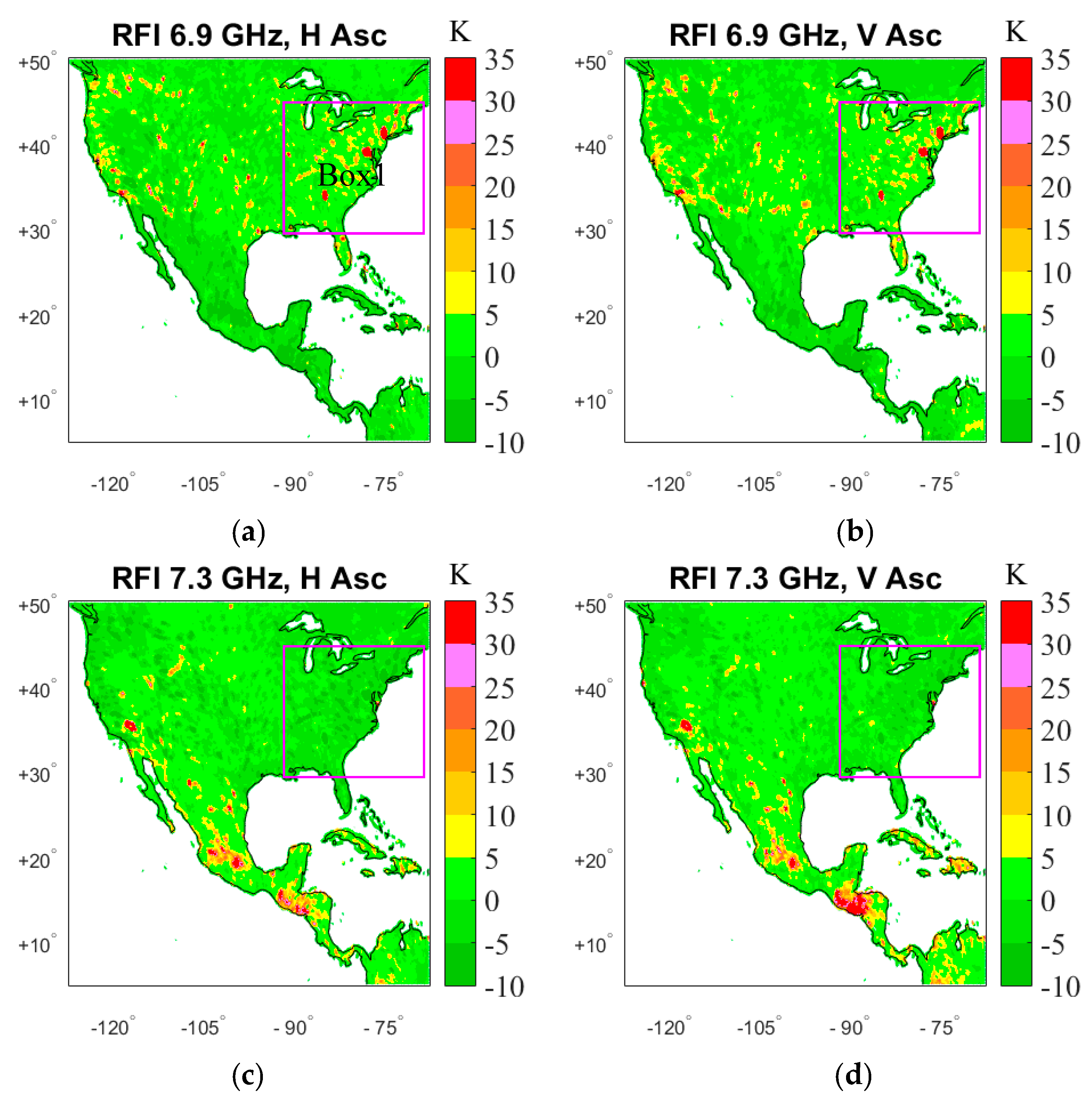
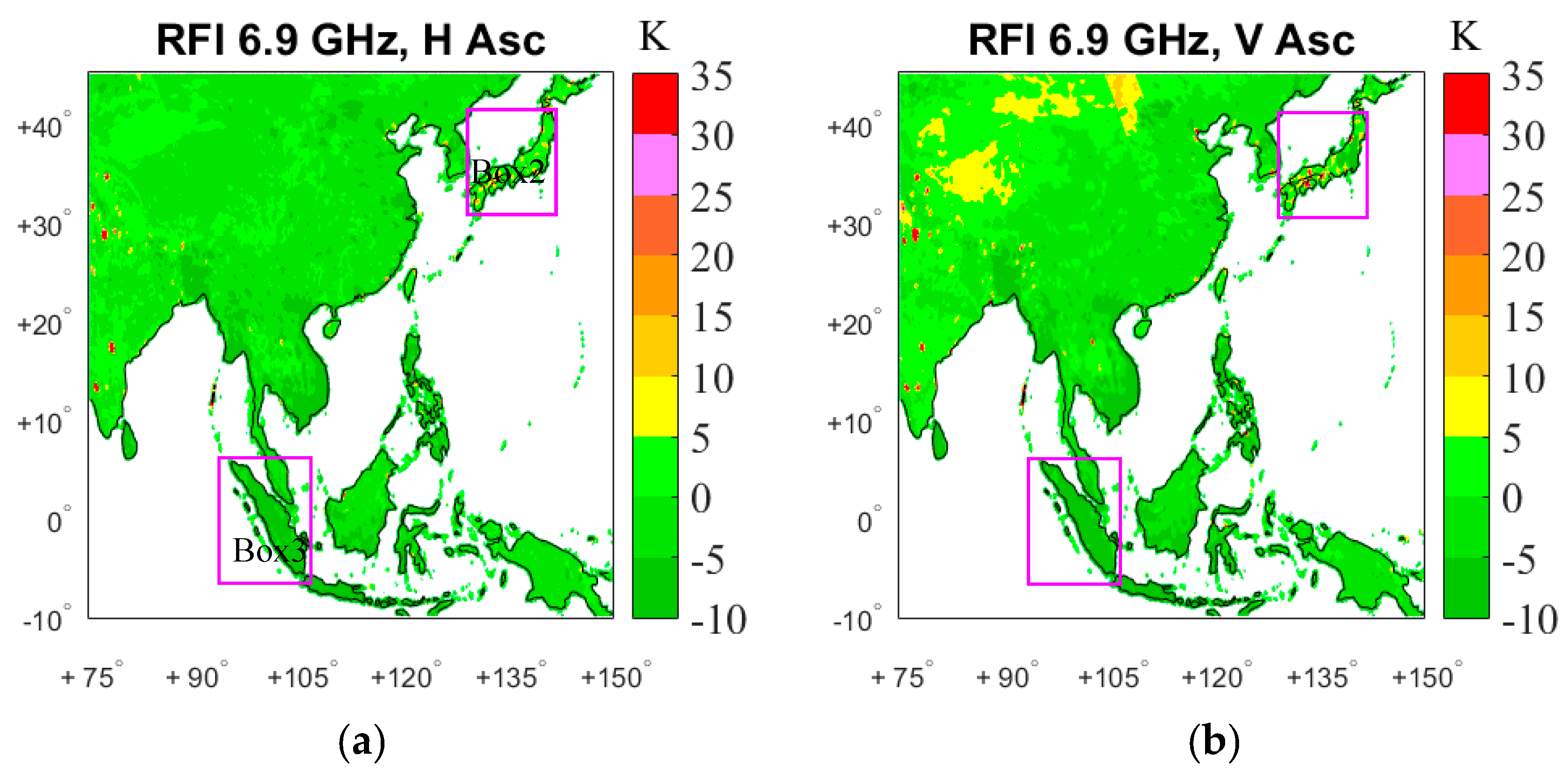
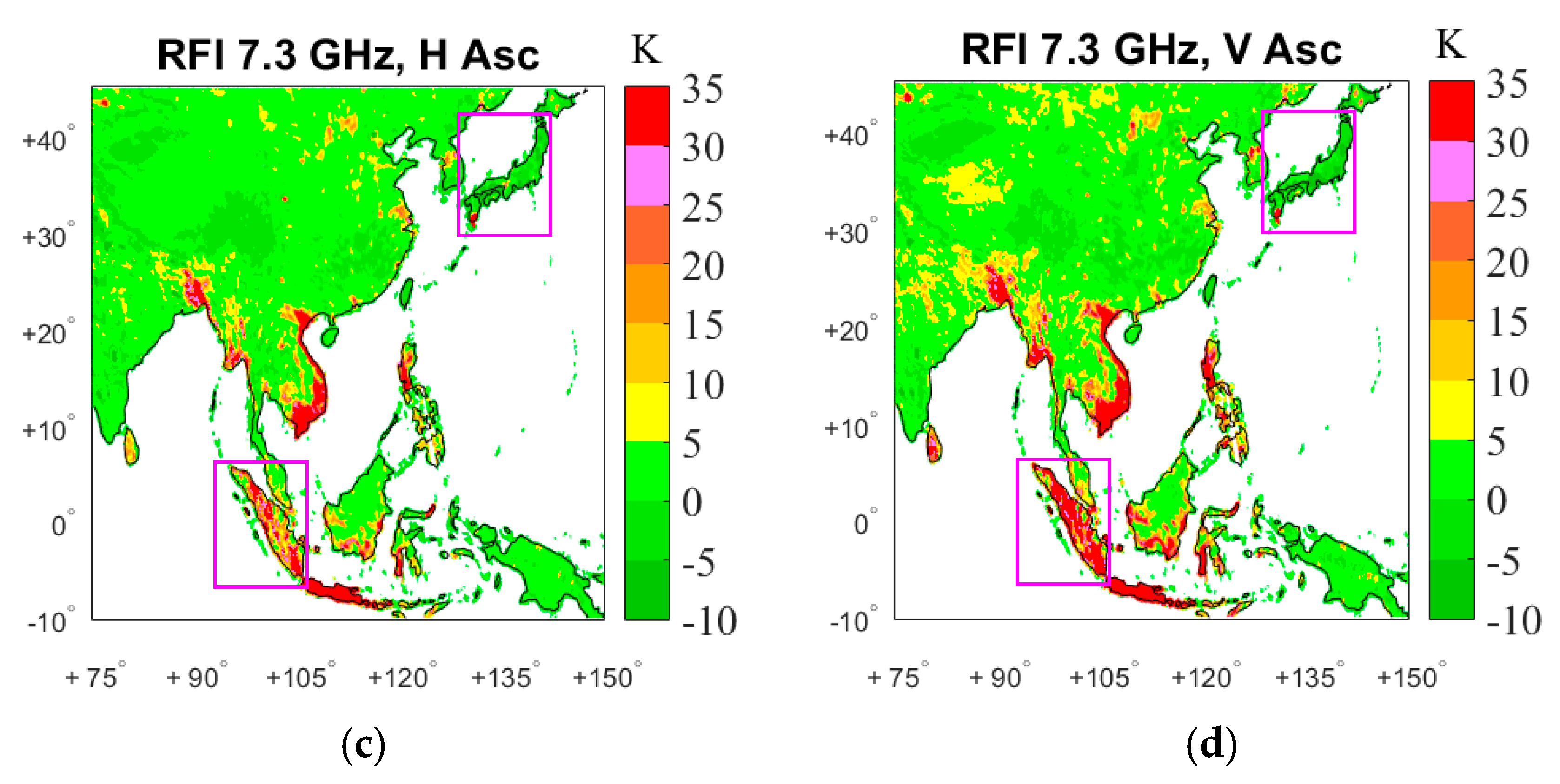
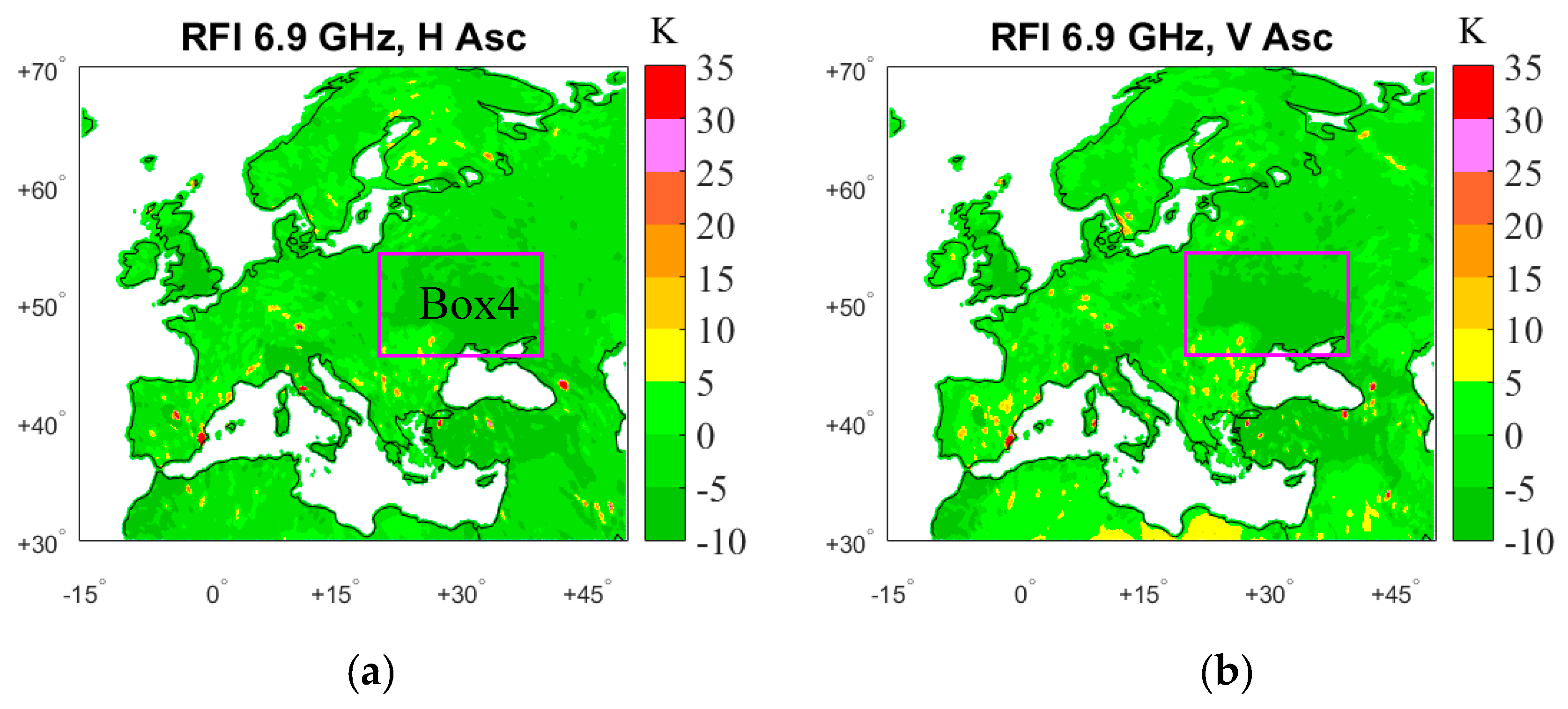
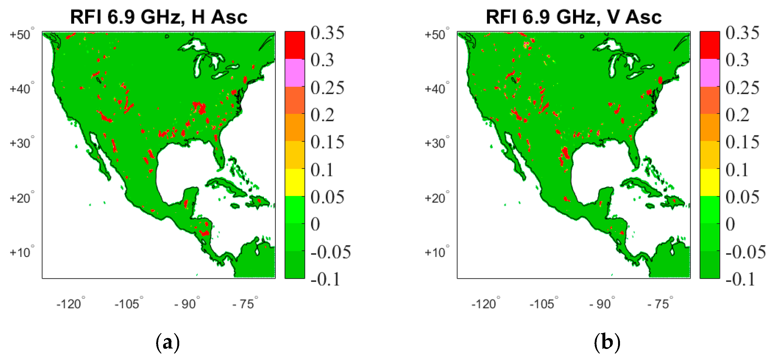
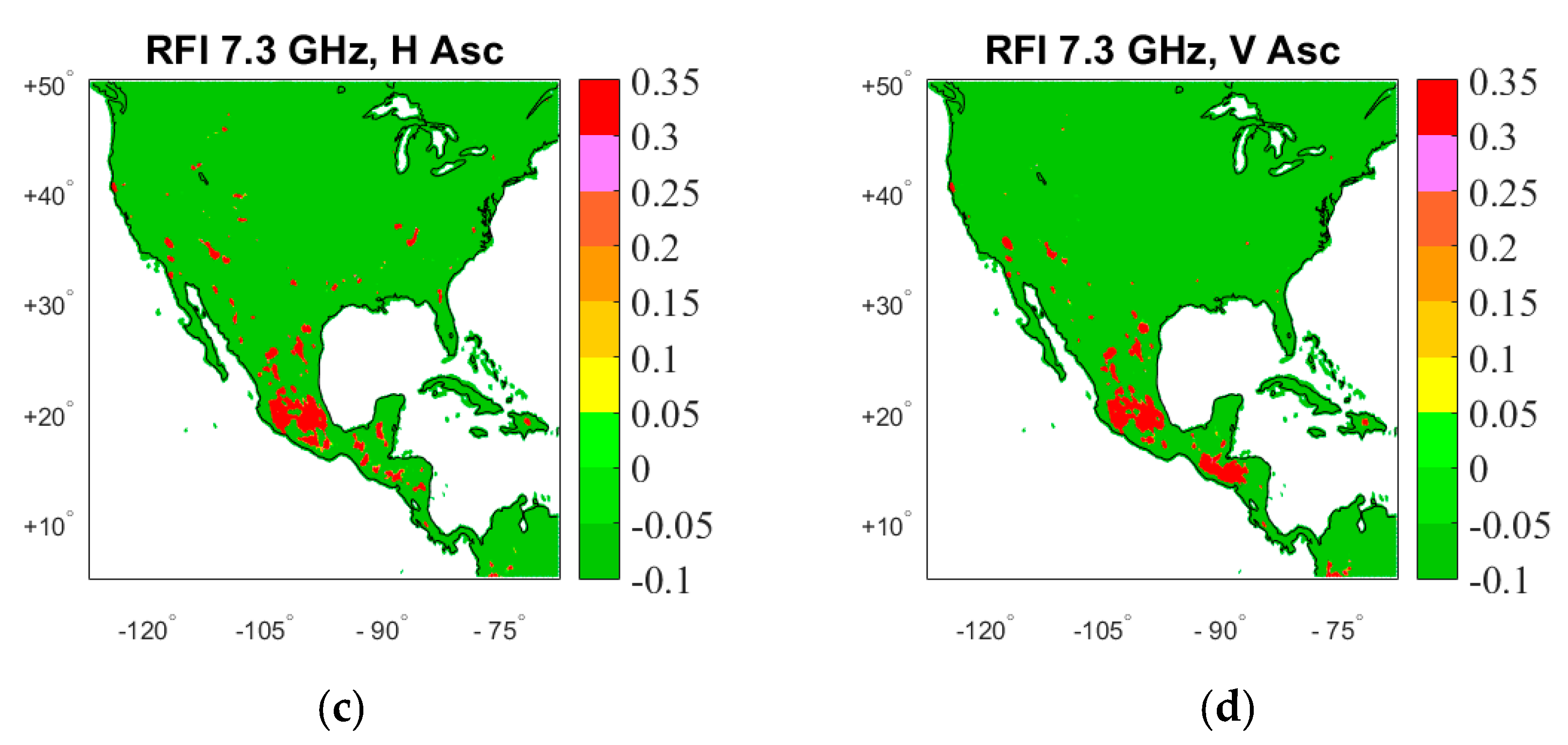
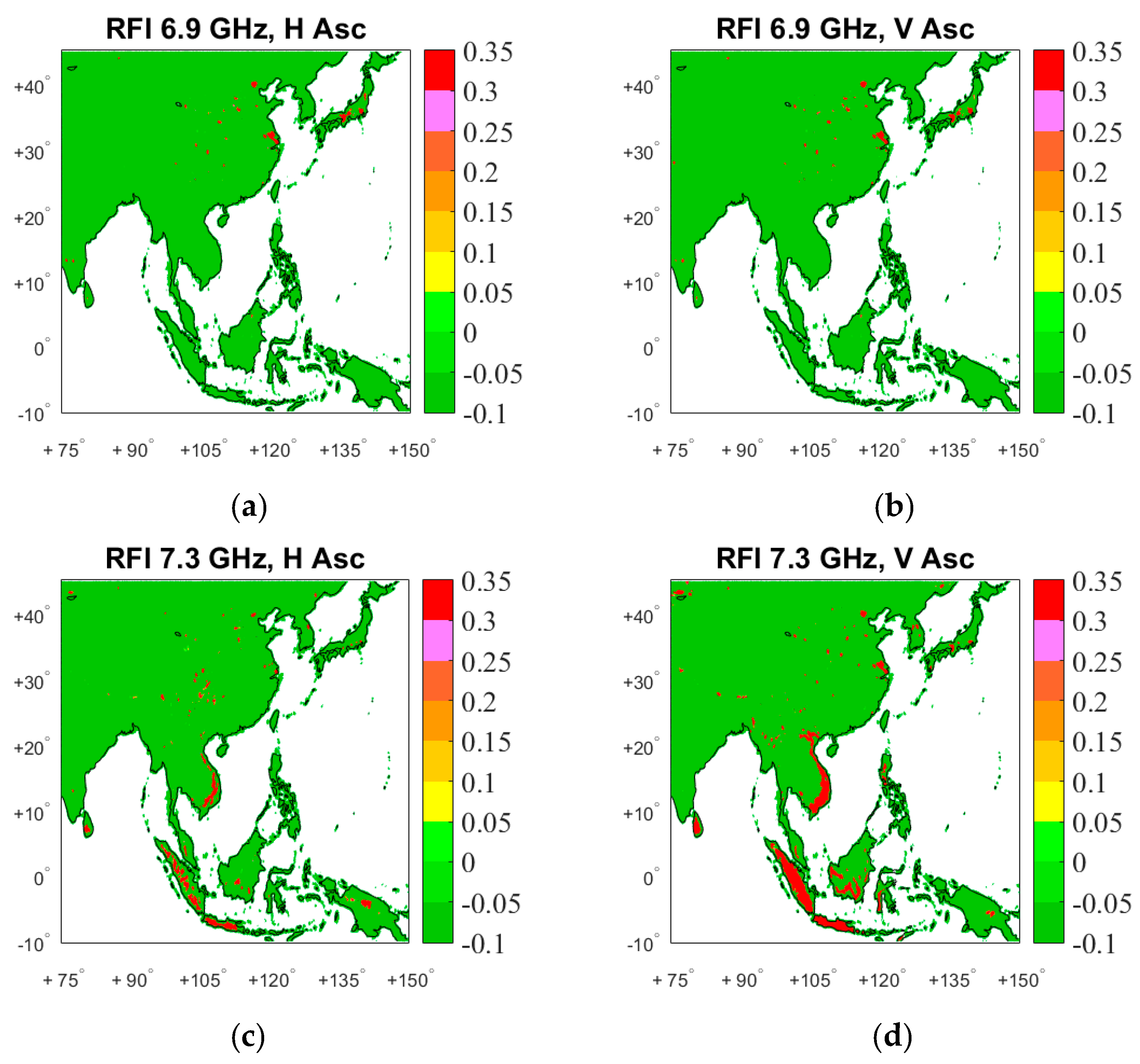
Figure 1, Figure 2 and Figure 3 show the spatial distribution of the generalized RFI index for the TB6H, TB6V, TB7H, and TB7V channels in the ascending orbits of AMSR2 that passed over North America, Southeast Asia, and Europe during 1–16 July 2017 (3-day average). Since RFI signals typically originate from a wide variety of coherent point target sources, they are often isolated in space and persistent in time. The areas where the generalized RFI index is abnormally large imply the presence of RFI, and the typical isolated features of RFI signals characterized by large positive generalized RFI index are found in many places.
Figure 1 shows that both horizontal and vertical polarization channels of 6.925 GHz over North America have strong RFI signals and are more densely distributed. The RFI signals generally appear in metropolitan areas of the United States and their adjacent regions—for example, in the east, such as Washington D. C., New York, and Boston; Los Angeles in the west; Denver in the center, and so forth. Meanwhile, Mexico is affected slightly by the 6.925 GHz RFI. However, almost no RFI is identified over the United States for the 7.3 GHz channels, except from areas around Washington D. C. and Los Angeles. In addition, relatively intense 7.3 GHz RFI signals appear over Mexico, Guatemala, and El Salvador, especially from Mexico City and Guatemala City. The RFI in 6.925 and 7.3 GHz channels have similar distributional characteristics in the descending orbits (figure omitted).
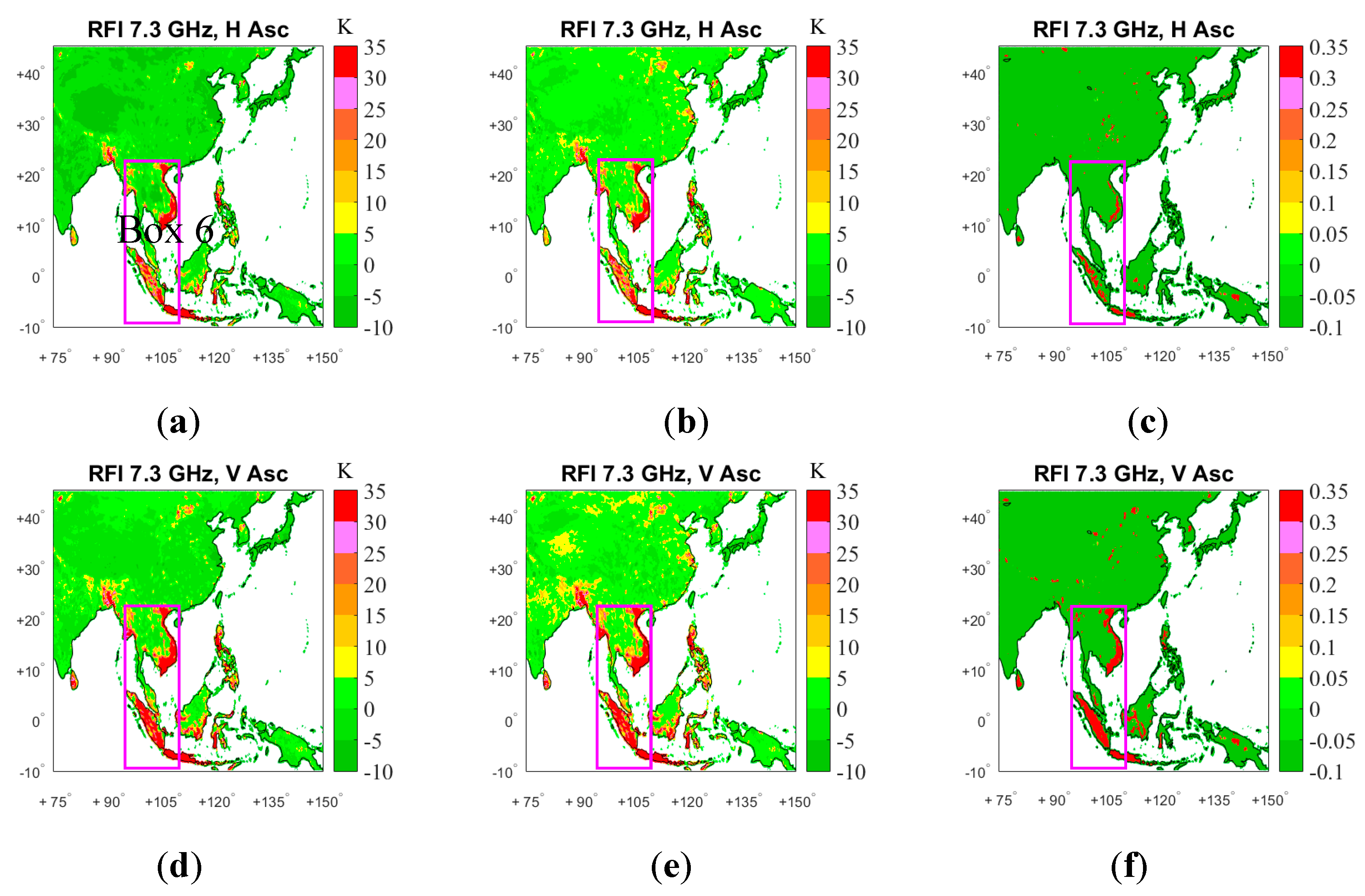
Figure 2 shows that RFI with high intensity from horizontal and vertical polarization channels of 6.925 GHz exists in Tokyo, Osaka, Okayama, and other locations in Japan. However, other places in Southeast Asia are not significantly influenced, and only sporadic RFI signals in this area are observed, including in Manila in the Philippines, Medan and Palembang in Indonesia, and New Delhi and Calicut in India, but other parts are basically unaffected.
However, for the 7.3 GHz channels, which belong to the C-band, at both horizontal and vertical polarization, and whether in ascending or descending orbit, the RFI distribution in Southeast Asia is much broader, for example, across Hebei in China, Seoul in Korea, Vietnam, Vientiane in Laos, Phnom Penh in Cambodia, Bangkok in Thailand, Naypyidaw, Yangon and Mandalay in Myanmar, Dhaka and Chittagong in Bangladesh, Colombo in Sri Lanka, Luzon’s west coast in the Philippines, Kuala Lumpur in Malaysia, Singapore, the islands of Sumatra and Java in Indonesia, and part of the Kalimantan and Sulawesi islands. All these areas are strongly contaminated with RFI, and the location and intensity of RFI do not change with time, meaning comparable levels of RFI contamination can be observed in each for these areas during 1–16 July. Moreover, the RFI at vertical polarization is stronger than that at horizontal polarization.
In Japan, RFI of the 7.3 GHz channels cannot be observed on every day in the 16 days from 1 July to 16 July 2017, and it appears on 2 July, 4 July, 6 July, 8 July, 11 July, 13 July, and 15 July (figure omitted). What makes it different is that the RFI of the 7.3 GHz channels in Japan always appears in ascending orbit observations, with no RFI contamination identified in descending orbit observations.
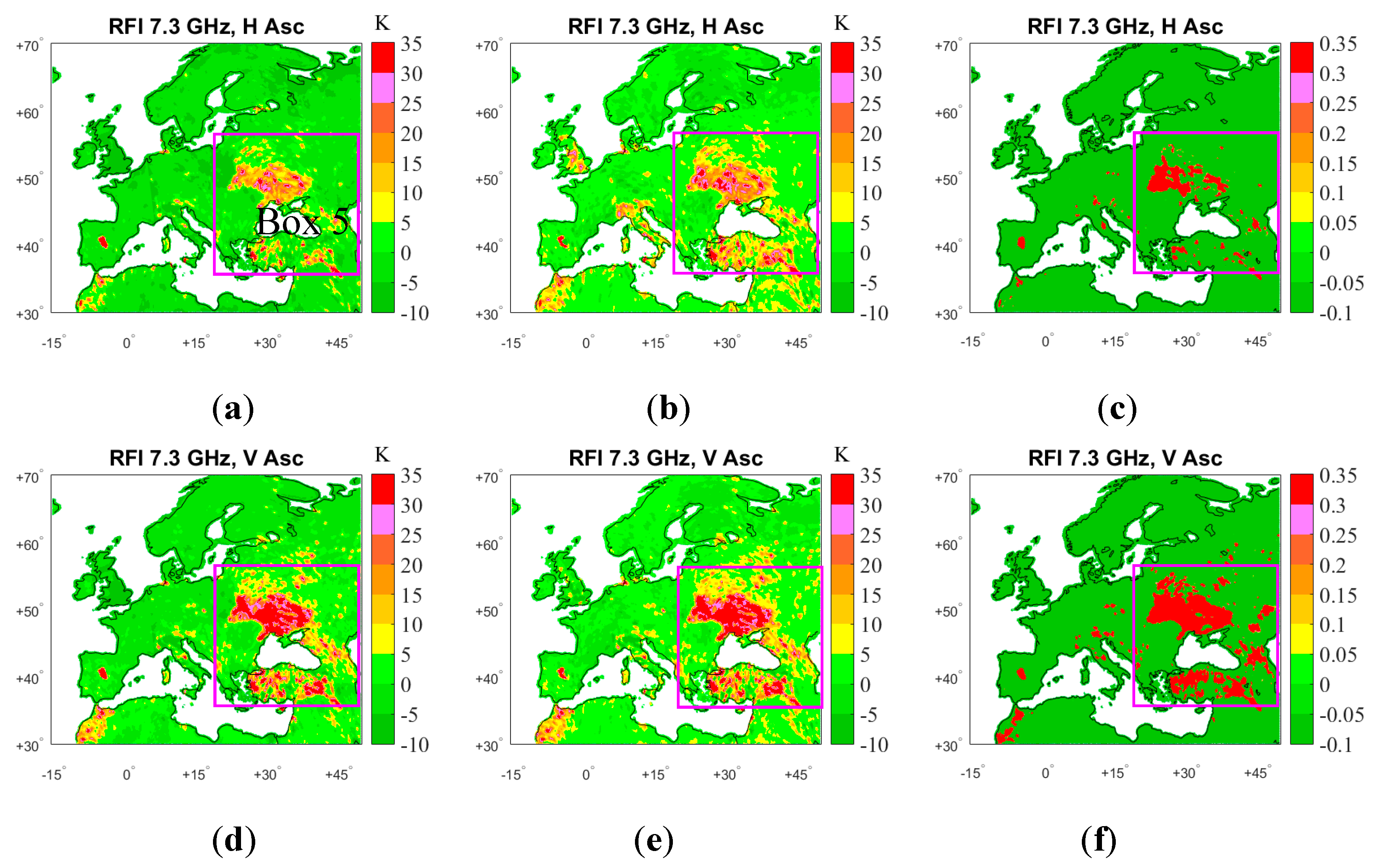
Figure 3 shows that the 6.925 GHz horizontal and vertical polarization channels are not significantly influenced by RFI in ascending orbits over Europe. However, in Spain, Germany, southern Europe (e.g., Romania, Hungary, Croatia, Bosnia and Herzegovina, Serbia, and Bulgaria), and Mediterranean coast there are some sparse RFI signals.
However, for the new 7.3 GHz C-band channels of AMSR2, especially at vertical polarization, the distribution of RFI in Europe is much broader. The distribution shows the RFI to be mainly concentrated over Belarus, Ukraine, Turkey, Georgia, and Iraq, but also Krasnodar and Makhachkala in southern Russia. The situation is similar in the descending orbit chart (figure omitted). In addition, near Madrid in Spain, four C-band low-frequency channels of AMSR2 are affected by RFI.
In addition, 7.3 GHz channel RFI is observed in South America, such as over Medellin in Columbia and Guayaquil in Ecuador; in Africa, such as over Morocco, Port Harcourt in Nigeria, and parts of South Africa, Zimbabwe, and Botswana; and in parts of Saudi Arabia in West Asia (figure omitted).
4.2. RFI Distribution Detected by the PCA Method
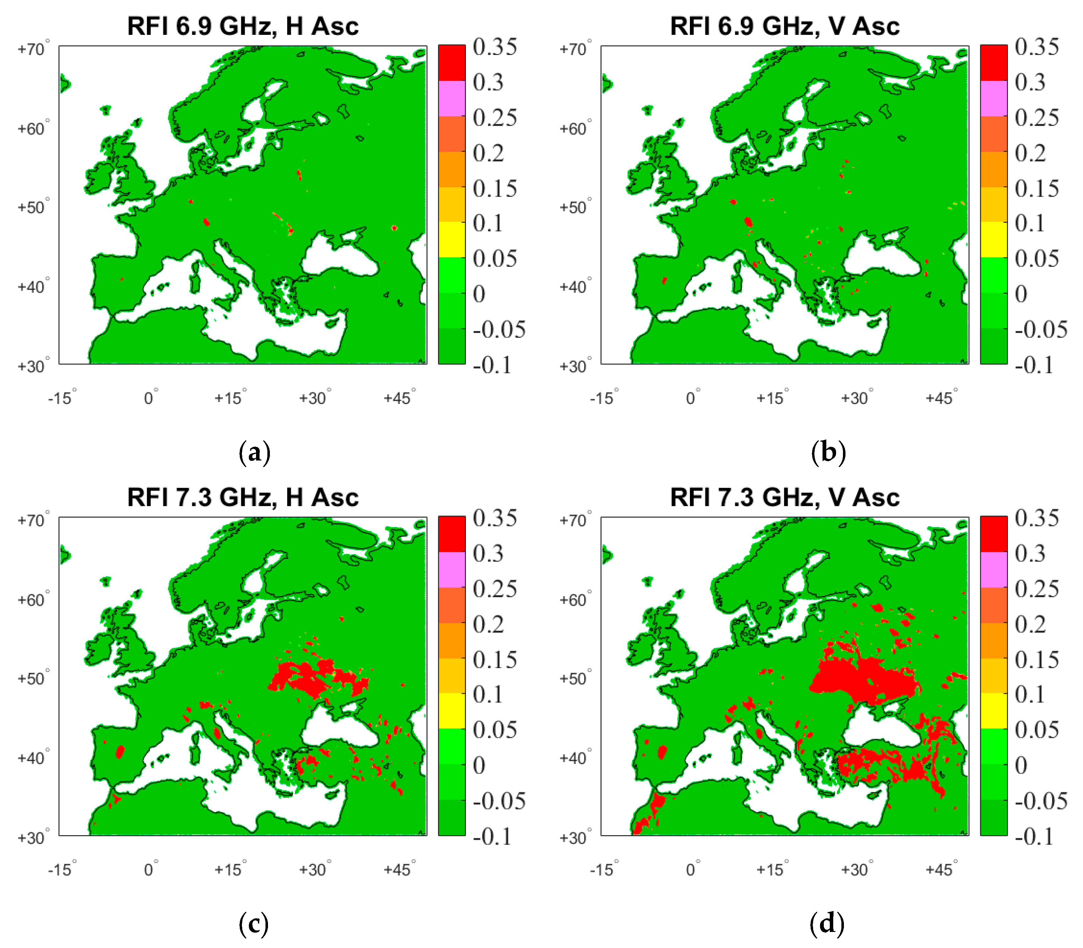
The PCA method is used to detect the distribution of C-band RFI signals over North America, Southeast Asia, and Europe. Based on the above PCA algorithm, the first PC coefficient, U1, related to RFI over land, is calculated. Figure 4, Figure 5 and Figure 6 show the spatial distribution of RFI signals in the AMSR2 6.925 and 7.3 GHz channels during 1–16 July 2017 (3-day average). In order to avoid misidentifying small- and medium-scale weather events as RFI signals, U1 > 0.3 is chosen as the PCA judgment RFI threshold.
The RFI of 6.925 GHz over North America is mainly distributed in the United States, while the 7.3 GHz RFI is mainly distributed in Mexico (Figure 4). In East Asia, the 6.925 GHz RFI mainly occurs over Japan, while the 7.3 GHz RFI is mainly distributed over China, South Korea, Japan, Vietnam, Indonesia, the Philippines, and Sri Lanka. Among them, the intensity of RFI over Vietnam, Indonesia, and Sri Lanka is much higher than that over other contaminated areas. Moreover, the RFI-contaminated areas over Vietnam and Indonesia’s islands of Sumatra and Java are very large, in good agreement with their national borders (Figure 5). In Europe, 6.925 GHz RFI is less distributed and its intensity is limited. However, 7.3 GHz RFI appears to be relatively large over Europe—mainly in France, Ukraine, and Turkey (Figure 6).
Comparing the RFI obtained using the generalized RFI detection method with that using the PCA method, the spatiotemporal characteristics are basically consistent with each other. The consistency between the two methods provides confidence that RFI may be reliably detected using either of the methods.
However, it is worth noting that the RFI-contaminated area identified by the PCA method is slightly smaller than that identified by the generalized RFI detection method in some regions, such as in Ukraine, Turkey, and especially the Philippines, Vietnam, Cambodia, and Myanmar in Southeast Asia.
To compare the two detection methods, Figure 7 and Figure 8 represent spatial distribution of observed RFI signals in ascending orbits at 7.3 GHz using spectral difference method, generalized RFI detection method, and PCA method over Europe and Southeast Asia during 14–16 July 2017. The numbers of observing pixels contaminated by RFI in Box 5 (Ukraine, Turkey and the vicinity), (35°–55°N, 20°–50°E), and Box 6 (the Indo-China Peninsula, the Malay peninsula, and the Sumatra Island), (10°S–22°N, 95°–110°E), are found in Table 3. RFI is detected when RFI index is larger than 5K using spectral difference method [25]. As well, RFI is detected when generalized RFI index is larger than 5K using generalized RFI detection method. Also, RFI is detected when the first PC coefficient is larger than 0.3 using PCA method. Based on Table 3, at 7.3 GHz channels, for both horizontal and vertical polarization, the generalized RFI detection method detected the most RFI-contaminated AMSR2 pixels, followed by the spectral difference method, and then the PCA method, which detected the least.
5. RFI Source Analysis
From the above results, Table 4 is put in to list the countries where RFI is observed over land.
It can be seen that the RFI-affected regions measured in AMSR2 6.925 GHz channels are mainly distributed in the United States, Japan, and India. Furthermore, RFI is found in the Philippines, Indonesia, and southern Europe, and sparser RFI is discovered over Rio de Janeiro and Santos in Brazil, South America, as well as some parts of southern Africa, such as Mbabane in Swaziland and Maseru in Lesotho (figure omitted). Under normal circumstances, the RFI intensity under vertical polarization conditions is greater than that under horizontal polarization conditions at the same frequency.
Regions affected by 7.3 GHz RFI are mainly distributed in Latin America, Southeast Asia, West Asia, Southern Europe, and Africa. The location of RFI in these areas does not change with time. In addition, the intensity of RFI at 7.3 GHz is stable in some areas, such as in Mexico City, Jakarta, and so on. Also, the RFI intensity varies with Earth azimuth angle of the field of view in some areas, such us in Kyiv, Port Harcourt, and so on. Moreover, the RFI at vertical polarization is stronger than the RFI at horizontal polarization. However, there is no obvious 7.3 GHz channel RFI over the United States and India, indicating that the new 7.3 GHz C-band channels of AMSR2 have been successful in relieving C-band RFI in these regions. Nonetheless, 7.3 GHz channel RFI is still found to exist in Japan, the position and intensity of which change over time. Furthermore, it always appears in the observations in ascending orbit, but not in descending orbit. Since specular reflections occur more frequently on the ocean surface when wind speeds are low, geosynchronous satellite signals also appear around a land mass, reflected from the ocean surface. Because AMSR2 is an instrument with the half-cone scanning characteristics, and geosynchronous satellites are over the equator, ascending data of regions north of the equator and descending data of regions south of the equator are likely contaminated by RFI which arises from geosynchronous satellite signals reflected from the ocean surface.
RFI signals are observed by AMSR2 in C-band mostly over industrial areas, scientific research centers, densely populated cities, ports, airports, and highways, indicating that the presence of RFI is always related to human activity and industrialization level.
The RFI observed by satellite-borne passive microwave sensors is either generated by ground-based radio-frequency transmitters, or arises from reflection of geosynchronous satellite signals over the Earth surface. The RFI emitted from ground-based active sources is often continuous over time, is relatively concentrated spatially, and affects both ascending and descending tracks. Furthermore, if the RFI intensity varies with the Earth azimuth observation angle, this indicates that the RFI probably originates from those ground-based transmitters with directional emission characteristics. In addition, since RFI over ocean surface usually arises from reflected signals such as those produced by transmitters on geosynchronous stationary satellites for telecommunication and television broadcast services [28], if the RFI intensity not only depends on the Earth azimuth angle of the field of view, but also on ascending/descending tracks of the satellite, it indicates that the RFI originates from geosynchronous satellite signals reflected from the ocean surface, especially over land near coastlines. These signals are reflected by the ocean surface and reach the AMSR2 radiometer antenna only under some specific geometric alignment of the geostationary satellites and the AMRS2 satellite platform.
For the terrestrial sources, the C-band channels of AMSR2 are usually used by, for example, Earth-to-space fixed-satellite services, space research services, space stations of the fixed-satellite services, geostationary satellite systems in the fixed-satellite service, and so on. However, the specific frequency bands used vary in different countries and regions [40].
Since AMSR2 is an advanced cone-scanning microwave instrument, its level-1 brightness temperature data provide the value of the Earth azimuth observation angle defined as the orientation of the satellite scanning direction relative to the north of the observed field of view, that is, the angle between the projection on the Earth of the connection which is between the observed field of view and the satellite and the true north direction, within the range of [−180°, 180°]. The clockwise azimuth is a positive value and the counterclockwise azimuth is a negative value.
The four regions in Figure 1, Figure 2 and Figure 3 are selected to discuss the relationship between the observation azimuth of the Earth and the magnitude of the brightness temperature. The geographic locations of the four regions are: Box 1 (Eastern United States), (30°–45°N, 70°–90°W); Box 2 (most of Japan), (30°–40°N, 130°–145°E); Box 3 (Sumatra Island and Peninsular Malaysia), (8°S–6°N, 90°–110°E); Box 4 (Ukraine and the vicinity), (45°–55°N, 20°–40°E).
Figure 9 is a scatterplot of the brightness temperature and Earth azimuth for the 6.925 and 7.3 GHz channels in the Box 1 (Eastern United States) region. It can be seen that, in this area, whether at vertical or horizontal polarization, or whether in ascending or descending orbit, the 6.925 GHz channels exhibit strong RFI. This also proves that 6.925 GHz RFI observed by AMSR2 in this area arises mainly from stable, continuous microwave transmitters. The significant RFI of the 7.3 GHz channel is only present at individual locations, which further demonstrates the positive effect of the new 7.3 GHz channel of AMSR2 compared with AMSR-E in mitigating the impact of C-band RFI over the United States.
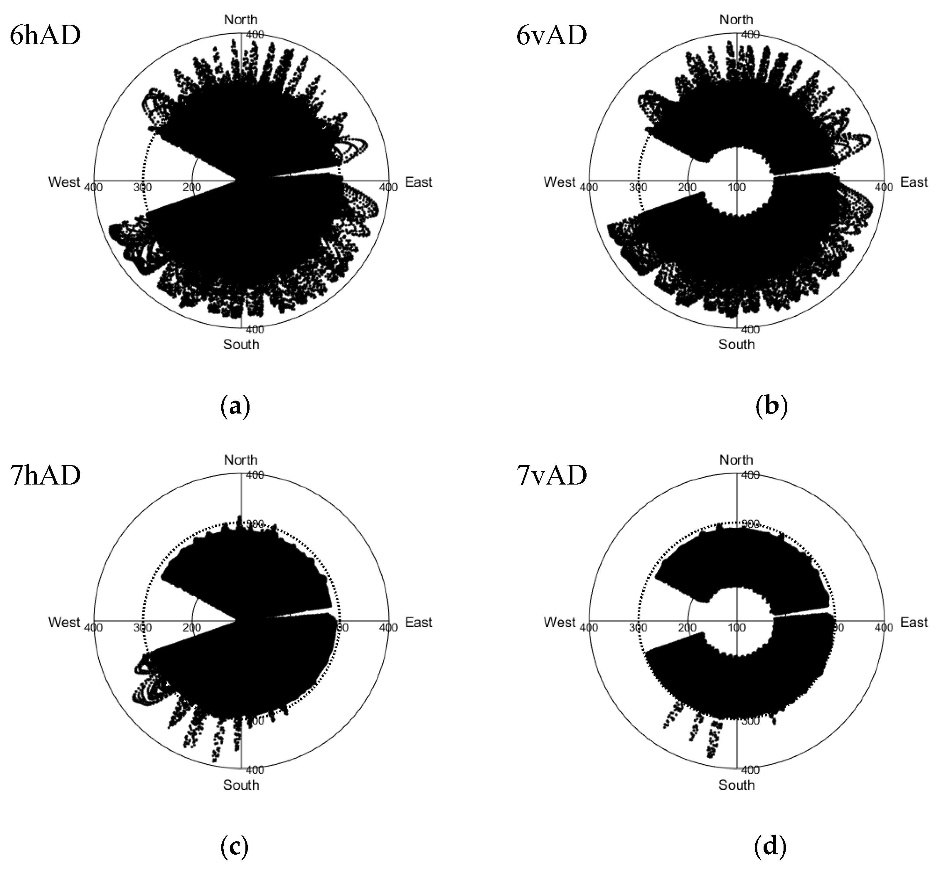
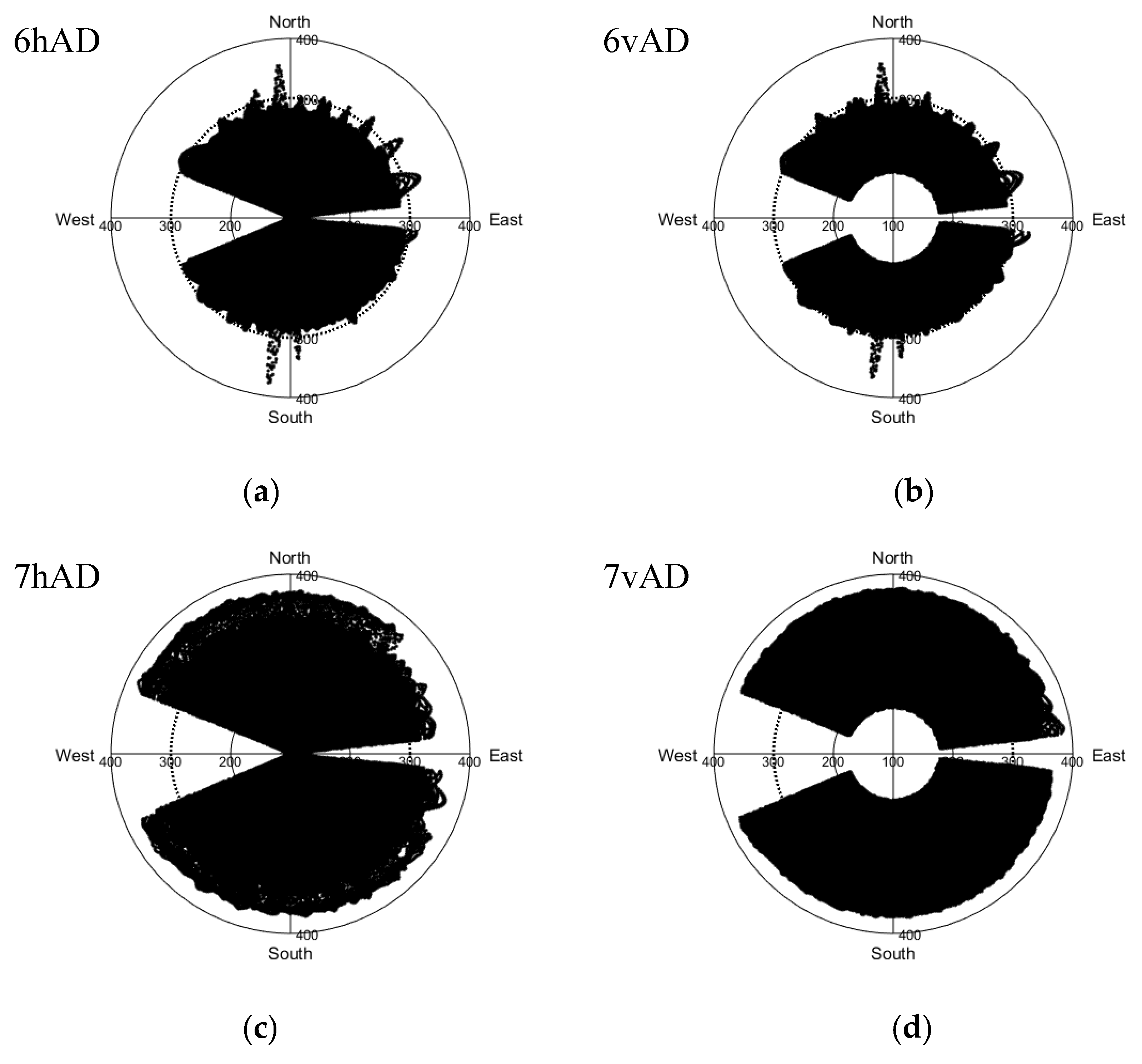
Shown in Figure 10 is a brightness temperature and Earth azimuth scatterplot for the 6.925 and 7.3 GHz channels in the Box 2 (most of Japan) region. From the horizontal and vertical polarizations in the area, the RFI of the 6.925 GHz channels appears in both ascending and descending orbits, and the intensity is greater when vertically polarized. This also proves that the RFI of 6.925 GHz channels in this area arises mainly from stable, continuous microwave transmitters. The location and intensity of 7.3 GHz RFI appear to be related to the azimuth of the Earth of the observed field of view; that is, only in some directions on ascending orbits is there strong RFI. Therefore, this RFI most likely arises from reflected radiation signals of geostationary satellites. Moreover, AMSR2 does not always suffer interference from geostationary satellite signals, and these fields of view are only affected by the RFI when the spaceborne passive microwave radiometer scans within a certain limited range of the azimuth of the Earth. Furthermore, multiple geosynchronous satellites could cause a range of RFI azimuth angles, but each satellite would have a different power level. In addition, since the RFI caused by ocean surface reflection depends very much on the relative geometrical position of geosynchronous satellites and the satellite on which passive instruments are carried, the nonstrict specular reflection gives the interference signal angular spread. The most prominent instance is analysis of the RFI over the Kyushu region of Japan, especially over Kagoshima of the Kyushu region.
It can be seen that the 7.3 GHz RFI only appears in a relatively narrow azimuthal range of [−180°, −110°] ∪ [120°, 180°] (Figure 10c,d). Combining the half-cone scanning characteristics of the AMSR2 instrument, that is, the azimuth of the Earth of the field of view in ascending orbit is in the range of [−180°, −90°] ∪ [90°, 180°], and that in descending orbit is [−90°, 90°], it can be seen that the range of the azimuth of the observed RFI is within the range of the azimuth of the field of view in ascending orbits. Here it is found again that the RFI of the 7.3 GHz channels always appears in ascending orbit observations over Japan, and no RFI contamination is identified in descending orbit observations. The azimuthal value in [120°, 180°] intervals is positive, indicating that all RFI-contaminated areas are on the left-hand side of the satellite’s flight direction. Meanwhile, the azimuthal value in [−180°, −110°] is negative, indicating all these RFI-contaminated areas are on the right-hand side of the satellite’s flight direction.
It also can be seen that the magnitude and the positive/negative values of the Earth azimuth angle of the field of view, corresponding to the observed RFI, are related to which side of the satellite flight direction the RFI-contaminated area is located. As far as ascending orbits, when the observational azimuth value is positive, the observed field of view of the RFI is on the left-hand side of the satellite’s flight direction; and the more to the left, the smaller the value of the azimuth. On the contrary, when the observational azimuth is negative, the observed field of view of the RFI is on the right-hand side of the satellite’s flight direction, and the smaller the absolute value of the negative value, the more to the right it is positioned. When a spaceborne passive microwave radiometer suffers interference from a reflected geostationary communication/television satellite signal, the location where RFI is observed has something to do with the Earth azimuth angle of the observed field of view and the position of the observed field of view relative to that of the geostationary satellite.
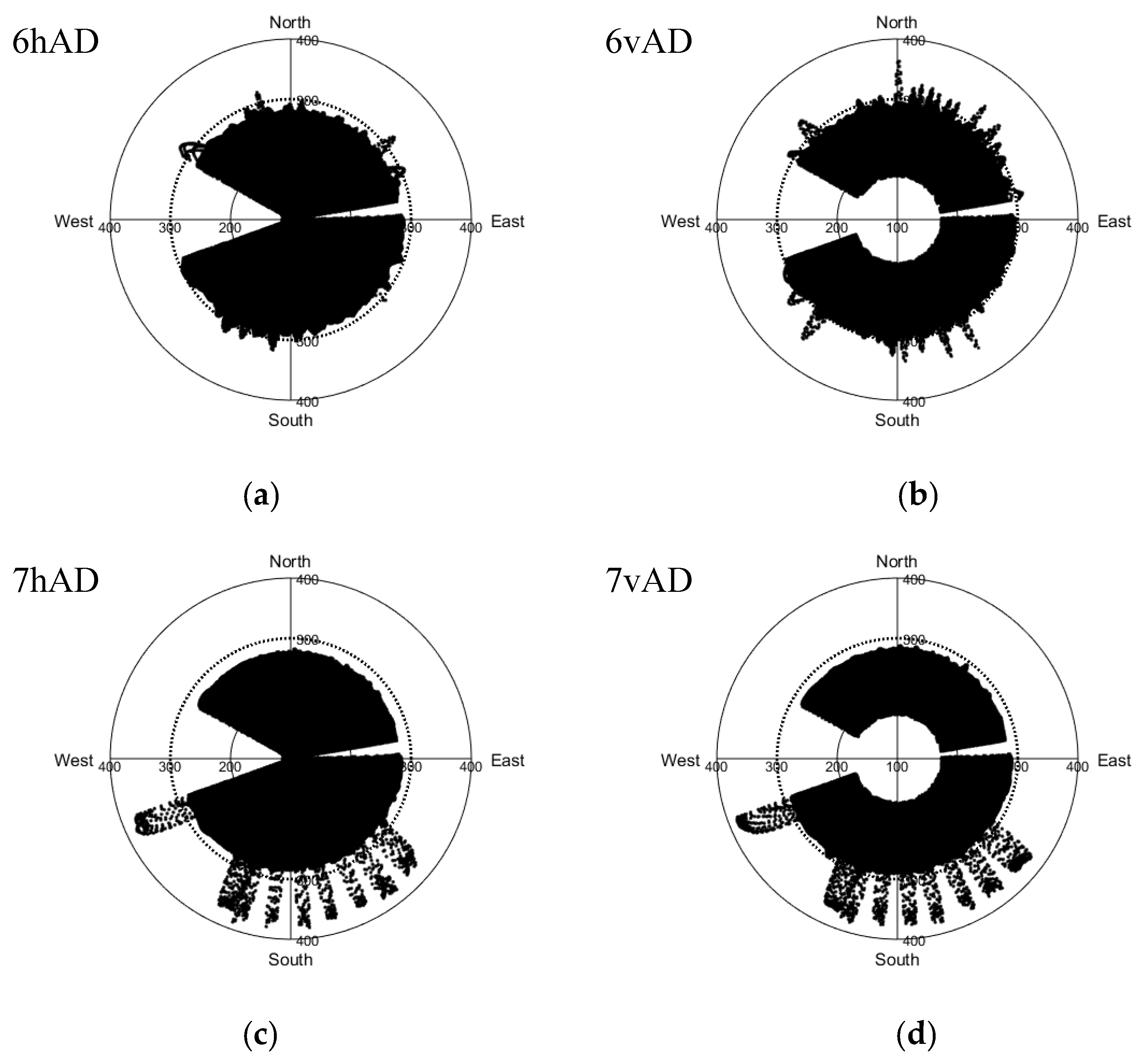
Taking the island of Sumatra in Indonesia as an example, Figure 11 shows a scatterplot of the brightness temperature and Earth azimuth of the 6.925 and 7.3 GHz channels in Box 3 (Sumatra Island and Peninsular Malaysia) of Figure 2a. As can be seen from Figure 11a,b, no matter which direction the instrument scans, the RFI of the 6.925 GHz channels in the Box 3 region can be observed almost all the time. Therefore, the field of view relevant to the RFI should be located throughout the whole azimuthal range that can be scanned by the microwave radiometer. As can be seen from Figure 11c,d, the azimuthal angle of the RFI-contaminated field of view of the 7.3 GHz channels in the Box 3 region is within the interval [−180°, −90°] and [90°, 180°]. It is evenly distributed, indicating that the position and intensity of the RFI appearing in Box 3 have nothing to do with the Earth azimuth angle. That is, the instrument has strong RFI contamination regardless of its direction. It can be seen that the RFI of the 7.3 GHz channel in Box 3 arises from stable and continuous ground-based active sources rather than reflective geostationary satellite signals. Moreover, the RFI of the 7.3 GHz channels in the Box 3 region is much stronger than that in the 6.925 GHz channels.
The RFI distribution in the Box 4 (Ukraine and the vicinity) region is similar to that of Box 3 (Sumatra Island and Peninsular Malaysia), except that the former has much less RFI in the 6.925 GHz channels than the latter, and the intensity is also smaller. The 7.3 GHz RFI has a similar Earth azimuth angle distributional to that of Box 3, but the intensity is also smaller (figure omitted).
6. Conclusions and Future Work
Based on AMSR2 brightness temperature data during 1–16 July 2017, the generalized RFI detection method and PCA method are used to detect C-band RFI signals over land, and the reasons for its occurrence are analyzed. The following conclusions are drawn:
(1) The RFI contamination of the C-band channel over land in summer identified by the generalized RFI detection method is basically the same as that by the PCA method. The identified location, intensity, and temporal variation characteristics of the RFI contamination are almost the same. This shows that the generalized RFI detection method and PCA algorithm are effective for identifying RFI over land (snow-free). However, the RFI-contaminated area identified by the PCA algorithm is smaller in some areas than that identified by the generalized RFI detection method, especially in Southeast Asia and Southern and Eastern Europe.
(2) Identified areas which are contaminated by 6.925 GHz RFI signals are basically consistent with previous analyses or references, and the areas usually do not coincide with those at 7.3 GHz. The regions with RFI-affected 7.3 GHz measurements are mainly distributed in Latin America, Southeast Asia, Western Asia, Southern Europe, and Africa. Moreover, there is no obvious RFI at 7.3 GHz in the United States and India, indicating that the addition of the new 7.3 GHz C-band channels in AMSR2 has been successful in relieving C-band RFI in these areas. However, the 7.3 GHz RFI still exists in Japan, and always appears in ascending orbit observations, but not at all in descending orbits.
(3) The stable, continuous RFI signals mainly arise from sustained and stable active microwave emitters on the ground, while the RFI signals that exhibit strong directionality, and for which intensity changes both with the Earth azimuth angle and scan track of the satellite, indicate that RFI contamination sources are mainly from reflected geostationary satellite signals.
The generalized RFI detection method is simplified. Meanwhile, characteristics of C-band RFI including spatial distribution, directional properties, and temporal variability were investigated using AMSR2 data. The comparison of the distribution and variability of RFI using two methods over land was made. The directional property of RFI was assessed using multiple observations at various azimuth angles. In some areas, the temporal variability of RFI is not as large as the directional differences. Furthermore, it is confirmed that the magnitude of RFI often depends on the direction of observation in these regions. Future work will quantify the levels of radiation that contaminate the AMSR2 C-band channels, and the same approach used here will be extended to sea surfaces and snow-covered land surface, as well as to X- and K-band measurements to have a comprehensive view of RFI contamination on AMSR2 radiances. Anyway, such a study may be useful for other missions working at these wavelengths as well as in localizing where these data have to be used with attention to the utilization of spaceborne passive microwave data and the inversion accuracy of geophysical parameters.
Author Contributions
Conceptualization: Y.W. and B.Q.; Methodology: Y.W.; Software: Y.W. and M.L.; Validation: Y.W., B.Q., and M.L.; Formal analysis: Y.W., Y.B., and G.P.P.; Investigation: M.L.; Resources: Y.B.; Data curation: X.L., L.L.; Writing—original draft preparation: Y.W.; Writing—review and editing: Y.B. and G.P.P.; Visualization: M.L.; Supervision: Y.B.; Project administration: Y.B.
Funding
This study was supported by the National Key Research and Development Program of China (2017YFC1501704), Jiangsu province basic research youth fund project of China (BK20150911), Pre-research project of SASTIND for the 13th Five-Year Plan (D010107), National Natural Science Foundation of China (41305033, 41675028) and Projects of Key Laboratory of Radiometric Calibration and Validation for Environmental Satellites, National Satellite Meteorological Center, China Meteorological Administration. G.P.P.’s participation was supported financially by the European Union’s Horizon 2020 Marie Skłodowska-Curie Project “ENViSIoN-EO” (grant agreement No 752094).
Acknowledgments
We thank the anonymous reviewers for the comments that helped improve our manuscript.
Conflicts of Interest
The authors declare no conflict of interest.
References
- Di Giuseppe, F.; Cesari, D.; Bonafe, G. Soil initialization strategy for use in limited-area weather prediction systems. Mon. Weather Rev. 2011, 139, 1844–1860. [Google Scholar] [CrossRef]
- Williams, I.N.; Lu, Y.; Kueppers, L.M.; Riley, W.J.; Biraud, S.C.; Bagley, J.E.; Torn, M.S. Land-atmosphere coupling and climate prediction over the U.S. Southern Great Plains. J. Geophys. Res. Atmos. 2016, 121. [Google Scholar] [CrossRef]
- Candy, B.; Saunders, R.W.; Ghent, D.; Bulgin, C.E. The impact of satellite-derived land surface temperatures on numerical weather prediction analyses and forecasts. J. Geophys. Res. Atmos. 2017, 122, 9783–9802. [Google Scholar] [CrossRef]
- Al-Yaari, A.; Dayau, S.; Chipeaux, C.; Aluome, C.; Kruszewski, A.; Loustau, D.; Wigneron, J.P. The AQUI Soil Moisture Network for Satellite Microwave Remote Sensing Validation in South-Western France. Remote Sens. 2018, 10, 1839. [Google Scholar] [CrossRef]
- Du, J.; Kimball, J.; Reichle, R.; Jones, L.; Watts, J.; Kim, Y. Global Satellite Retrievals of the Near-Surface Atmospheric Vapor Pressure Deficit from AMSR-E and AMSR2. Remote Sens. 2018, 10, 1175. [Google Scholar] [CrossRef] [PubMed]
- Pavelin, E.G.; Candy, B. Assimilation of surface-sensitive infrared radiances over land: Estimation of land surface temperature and emissivity. Q. J. R. Meteorol. Soc. 2014, 140, 1198–1208. [Google Scholar] [CrossRef]
- Xie, Y.; Shi, J.; Lei, Y.; Li, Y. Modeling Microwave Emission from Short Vegetation-Covered Surfaces. Remote Sens. 2015, 7, 14099–14118. [Google Scholar] [CrossRef] [Green Version]
- De Rosnay, P.; Drusch, M.; Vasiljevic, D.; Balsamo, G.; Albergel, C.; Isaksen, L. A simplified extended Kalman filter for the global operational soil moisture analysis at ECMWF. Q. J. R. Meteorol. Soc. 2013, 139, 1199–1213. [Google Scholar] [CrossRef]
- Martin, G.M.; Milton, S.F.; Senior, C.A.; Brooks, M.E.; Ineson, S. Analysis and reduction of systematic errors through a seamless approach to modeling weather and climate. J. Clim. 2010, 23, 5933–5957. [Google Scholar] [CrossRef]
- Berg, W.; Kroodsma, R.; Kummerow, C.; McKague, D. Fundamental Climate Data Records of Microwave Brightness Temperatures. Remote Sens. 2018, 10, 1306. [Google Scholar] [CrossRef]
- Du, J.; Kimball, J.; Shi, J.; Jones, L.; Wu, S.; Sun, R.; Yang, H. Inter-Calibration of Satellite Passive Microwave Land Observations from AMSR-E and AMSR2 Using Overlapping FY3B-MWRI Sensor Measurements. Remote Sens. 2014, 6, 8594–8616. [Google Scholar] [CrossRef] [Green Version]
- Shi, J.; Du, Y.; Du, J.; Jiang, L.; Chai, L.; Mao, K.; Xu, P.; Ni, W.; Xiong, C.; Liu, Q.; et al. Progresses on microwave remote sensing of land surface parameters. Sci. China Earth Sci. 2012, 55, 1052–1078. (In Chinese) [Google Scholar] [CrossRef]
- Kidd, C. Radio frequency interference at passive microwave earth observation frequencies. Int. J. Remote Sens. 2006, 27, 3853–3865. [Google Scholar] [CrossRef]
- Li, L.; Njoku, E.G.; Im, E.; Chang, P.S.; Germain, K.S. A preliminary survey of Radio-Frequency Interference over the U.S. in Aqua AMSR-E data. IEEE Trans. Geosci. Remote Sens. 2004, 42, 380–390. [Google Scholar] [CrossRef]
- Njoku, E.G.; Ashcroft, P.; Chan, T.K.; Li, L. Global survey and statistics of Radio-Frequency Interference in AMSR-E land observations. IEEE Trans. Geosci. Remote Sens. 2005, 43, 938–947. [Google Scholar] [CrossRef]
- Li, L.; Gaiser, P.W.; Bettenhausen, M.H.; Johnston, W. WindSat radio-frequency interference signature and its identification over land and ocean. IEEE Trans. Geosci. Remote Sens. 2006, 44, 530–539. [Google Scholar] [Green Version]
- Yang, H.; Weng, F. Error sources in remote sensing of microwave land surface emissivity. IEEE Trans. Geosci. Remote Sens. 2011, 49, 3437–3442. [Google Scholar] [CrossRef]
- Wu, Y.; Weng, F. Applications of an AMSR-E RFI detection and correction algorithm in 1-DVAR over land. J. Meteo. Res. 2014, 28, 645–655. [Google Scholar]
- Zou, X.; Zhao, J.; Weng, F.; Qin, Z. Detection of Radio-Frequency Interference signal over land from FY-3B Microwave Radiation Imager (MWRI). IEEE Trans. Geosci. Remote Sens. 2012, 40, 4994–5003. [Google Scholar] [CrossRef]
- Kachi, M.; Imaoka, K.; Fujii, H.; Shibata, A.; Kasahara, M.; Iida, Y.; Ito, N.; Nakagawa, K.; Shimoda, H. Status of GCOM-W1/AMSR2 development and science activities. In Sensors, Systems, and Next-Generation Satellites XII; International Society for Optics and Photonics: Bellingham, WA, USA, 2008. [Google Scholar]
- Draper, D.; Newell, D. An assessment of Radio Frequency Interference using the GPM Microwave Imager. In Proceedings of the 2015 IEEE International Geoscience and Remote Sensing Symposium (IGARSS), Milan, Italy, 26–31 July 2015. [Google Scholar]
- Grenkov, S.A.; Kol’tsov, N.E. Spectral-Selective Radiometer Unit with Radio-Interference Protection. Radiophys. Quantum Electron. 2015, 58, 520–528. [Google Scholar] [CrossRef]
- Ellingson, S.W.; Johnson, J.T. A polarimetric survey of radio-frequency interference in C-and X-bands in the continental United States using WindSat radiometry. IEEE Trans. Geosci. Remote Sens. 2006, 44, 540–548. [Google Scholar] [CrossRef]
- Johnson, J.T.; Gasiewski, A.J.; Guner, B.; Hampson, G.A.; Ellingson, S.W.; Krishnamachari, R.; Niamsuwan, N.; McIntyre, E.; Klein, M.; Leuski, V.Y. Airborne radio-frequency interference studies at C band using a digital receiver. IEEE Trans. Geosci. Remote Sens. 2006, 44, 1974–1985. [Google Scholar] [CrossRef]
- Ruf, C.S.; Gross, S.M.; Misra, S. RFI detection and mitigation for microwave radiometry with an agile digital detector. IEEE Trans. Geosci. Remote Sens. 2006, 44, 694–706. [Google Scholar] [CrossRef]
- Piepmeier, J.R.; Mohammed, P.N.; Knuble, J.J. A double detector for RFI mitigation in microwave radiometers. IEEE Trans. Geosci. Remote Sens. 2008, 46, 458–465. [Google Scholar] [CrossRef]
- McKague, D.; Puckett, J.J.; Ruf, C. Characterization of K-band radio frequency interference from AMSR-E, WindSat and SSM/I. In Proceedings of the 2010 IEEE International Geoscience and Remote Sensing Symposium, Honolulu, HI, USA, 25–30 July 2010; pp. 2492–2494. [Google Scholar]
- Wu, Y.; Weng, F. Detection and Correction of AMSR-E Radio-Frequency Interference. Acta Meteorol. Sin. 2011, 25, 669–681. [Google Scholar] [CrossRef]
- Guan, L.; Zhang, S. Source analysis of spaceborne microwave radiometer interference over land. Front. Earth Sci. 2016, 10, 135–144. [Google Scholar] [CrossRef]
- Metelev, S.; Lvov, A. Estimation of the Potential Interference Immunity of Radio Reception with Spatial Signal Processing in Multipath Radio-Communication Channels. I. Decameter Range. Radiophys. Quantum Electron. 2016, 59, 329–340. [Google Scholar] [CrossRef]
- Adams, I.S.; Bettenhausen, M.H.; Gaiser, P.W.; Johnston, W. Identification of ocean-reflected radio-frequency interference using WindSat retrieval chi-square probability. IEEE Geosci. Remote Sens. Lett. 2010, 7, 406–410. [Google Scholar] [CrossRef]
- Zhao, J.; Zou, X.; Weng, F. WindSat radio-frequency interference signature and its identification over Green land and Antarctic. IEEE Trans. Geosci. Remote Sens. 2013, 51, 4830–4839. [Google Scholar] [CrossRef]
- Lacava, T.; Coviello, I.; Faruolo, M.; Mazzeo, G.; Pergola, N.; Tramutoli, V. A multitemporal investigation of AMSR-E C-band radio-frequency interference. IEEE Trans. Geosci. Remote Sens. 2013, 51, 2007–2015. [Google Scholar] [CrossRef]
- Guner, B.; Johnson, J.T.; Niamsuwan, N. Time and frequency blanking for radio-frequency interference mitigation in microwave radiometry. IEEE Trans. Geosci. Remote Sens. 2007, 45, 3672–3679. [Google Scholar] [CrossRef]
- Hallikainen, M.; Kainulainen, J.; Seppänen, J.; Hakkarainen, A.; Rautiainen, K. Studies of radio frequency interference at L-band using an airborne 2-D interferometric radiometer. In Proceedings of the 2010 IEEE International Geoscience and Remote Sensing Symposium, Honolulu, HI, USA, 25–30 July 2010. [Google Scholar]
- Misra, S.; Ruf, C.S. Analysis of radio frequency interference detection algorithms in the angular domain for SMOS. IEEE Trans. Geosci. Remote Sens. 2012, 50, 1448–1457. [Google Scholar] [CrossRef]
- Zou, X.; Tian, X.; Weng, F. Detection of television frequency interference with satellite microwave imager observations over oceans. J. Atmos. Ocean. Technol. 2014, 31, 2759–2776. [Google Scholar] [CrossRef]
- Zabolotskikh, E.V.; Mitnik, L.M.; Chapron, B. Radio-Frequency Interference Identification Over Oceans for C- and X-Band AMSR2 Channels. IEEE Geosci. Remote Sens. Lett. 2015, 12, 1705–1709. [Google Scholar] [CrossRef]
- Tian, X.; Zou, X. An Empirical Model for Television Frequency Interference Correction of AMSR2 Data Over Ocean Near the U.S. and Europe. IEEE Trans. Geosci. Remote Sens. 2016, 54, 3856–3867. [Google Scholar] [CrossRef]
- Radio Spectrum Allocation. Available online: https://www.fcc.gov/engineering-technology/policy-and-rules-division/general/radio-spectrum-allocation (accessed on 8 May 2019).
Figure 1.
Spatial distribution of RFI signals observed by AMSR2 in ascending orbits at (a,b) 6.925 GHz and (c,d) 7.3 GHz, at (a,c) horizontal and (b,d) vertical polarization, using the generalized RFI detection approach over North America during 1–16 July 2017.
Figure 1.
Spatial distribution of RFI signals observed by AMSR2 in ascending orbits at (a,b) 6.925 GHz and (c,d) 7.3 GHz, at (a,c) horizontal and (b,d) vertical polarization, using the generalized RFI detection approach over North America during 1–16 July 2017.

Figure 2.
As in Figure 1 but for Southeast Asia during 1–16 July 2017. (a) 6.925 GHz horizontal polarization, (b) 6.925 GHz vertical polarization, (c) 7.3 GHz horizontal polarization, (d) 7.3 GHz vertical polarization.
Figure 2.
As in Figure 1 but for Southeast Asia during 1–16 July 2017. (a) 6.925 GHz horizontal polarization, (b) 6.925 GHz vertical polarization, (c) 7.3 GHz horizontal polarization, (d) 7.3 GHz vertical polarization.


Figure 3.
As in Figure 1 but for Europe during 1–16 July 2017. (a) 6.925 GHz horizontal polarization, (b) 6.925 GHz vertical polarization, (c) 7.3 GHz horizontal polarization, (d) 7.3 GHz vertical polarization.
Figure 3.
As in Figure 1 but for Europe during 1–16 July 2017. (a) 6.925 GHz horizontal polarization, (b) 6.925 GHz vertical polarization, (c) 7.3 GHz horizontal polarization, (d) 7.3 GHz vertical polarization.


Figure 4.
PCA-based RFI distribution in descending orbits at (a,b) 6.925 GHz and (c,d) 7.3 GHz, at (a,c) horizontal and (b,d) vertical polarization, over North America during 1–16 July 2017.
Figure 4.
PCA-based RFI distribution in descending orbits at (a,b) 6.925 GHz and (c,d) 7.3 GHz, at (a,c) horizontal and (b,d) vertical polarization, over North America during 1–16 July 2017.


Figure 5.
As in Figure 4 but for Southeast Asia during 1–16 July 2017. (a) 6.925 GHz horizontal polarization, (b) 6.925 GHz vertical polarization, (c) 7.3 GHz horizontal polarization, (d) 7.3 GHz vertical polarization.
Figure 5.
As in Figure 4 but for Southeast Asia during 1–16 July 2017. (a) 6.925 GHz horizontal polarization, (b) 6.925 GHz vertical polarization, (c) 7.3 GHz horizontal polarization, (d) 7.3 GHz vertical polarization.

Figure 6.
As in Figure 4 but for Europe during 1–16 July 2017. (a) 6.925 GHz horizontal polarization, (b) 6.925 GHz vertical polarization, (c) 7.3 GHz horizontal polarization, (d) 7.3 GHz vertical polarization.
Figure 6.
As in Figure 4 but for Europe during 1–16 July 2017. (a) 6.925 GHz horizontal polarization, (b) 6.925 GHz vertical polarization, (c) 7.3 GHz horizontal polarization, (d) 7.3 GHz vertical polarization.

Figure 7.
Spatial distribution of RFI signals observed by AMSR2 in ascending orbits at 7.3 GHz, at (a–c) horizontal and (d–f) vertical polarization, using spectral difference method (a,d), generalized RFI detection method (b,e), and PCA method (c,f) over Europe during 14–16 July 2017.
Figure 7.
Spatial distribution of RFI signals observed by AMSR2 in ascending orbits at 7.3 GHz, at (a–c) horizontal and (d–f) vertical polarization, using spectral difference method (a,d), generalized RFI detection method (b,e), and PCA method (c,f) over Europe during 14–16 July 2017.

Figure 8.
Spatial distribution of RFI signals observed by AMSR2 in ascending orbits at 7.3 GHz, at (a–c) horizontal and (d–f) vertical polarization, using spectral difference method (a,d), generalized RFI detection method (b,e), and PCA method (c,f) over Southeast Asia during 14–16 July 2017.
Figure 8.
Spatial distribution of RFI signals observed by AMSR2 in ascending orbits at 7.3 GHz, at (a–c) horizontal and (d–f) vertical polarization, using spectral difference method (a,d), generalized RFI detection method (b,e), and PCA method (c,f) over Southeast Asia during 14–16 July 2017.

Figure 9.
The relationship between the brightness temperature and the Earth azimuth observation angle of AMSR2 in Box 1 (Eastern United States) during 1–16 July 2017. (a) 6.925 GHz horizontal polarization, (b) 6.925 GHz vertical polarization, (c) 7.3 GHz horizontal polarization, (d) 7.3 GHz vertical polarization.

Figure 10.
As in Figure 9 but for Box 2 (most of Japan) during 1–16 July 2017. (a) 6.925 GHz horizontal polarization, (b) 6.925 GHz vertical polarization, (c) 7.3 GHz horizontal polarization, (d) 7.3 GHz vertical polarization.
Figure 10.
As in Figure 9 but for Box 2 (most of Japan) during 1–16 July 2017. (a) 6.925 GHz horizontal polarization, (b) 6.925 GHz vertical polarization, (c) 7.3 GHz horizontal polarization, (d) 7.3 GHz vertical polarization.

Figure 11.
As in Figure 9 but for Box 3 (Sumatra Island and Peninsular Malaysia) during 1–16 July 2017. (a) 6.925 GHz horizontal polarization, (b) 6.925 GHz vertical polarization, (c) 7.3 GHz horizontal polarization, (d) 7.3 GHz vertical polarization.
Figure 11.
As in Figure 9 but for Box 3 (Sumatra Island and Peninsular Malaysia) during 1–16 July 2017. (a) 6.925 GHz horizontal polarization, (b) 6.925 GHz vertical polarization, (c) 7.3 GHz horizontal polarization, (d) 7.3 GHz vertical polarization.


Table 1.
AMSR2 channel characteristics.
| Center Freq./GHz | Pol. | Band Width/MHz | Ground Res./km | Sensitivity/K |
|---|---|---|---|---|
| 6.925 | H/V | 350 | 35 × 62 | 0.34 |
| 7.3 | H/V | 350 | 34 × 58 | 0.43 |
| 10.65 | H/V | 100 | 24 × 42 | 0.7 |
| 18.7 | H/V | 200 | 14 × 22 | 0.7 |
| 23.8 | H/V | 400 | 15 × 26 | 0.6 |
| 36.5 | H/V | 1000 | 7 × 12 | 0.7 |
| 89.0 | H/V | 3000 | 3 × 5 | 1.2 |
Table 2.
Concrete coefficients in Equation (2).
| Coefficients in Equation (2) | ΔTb[i] | |||
|---|---|---|---|---|
| ΔTb[1] (i = 1) | ΔTb[2] (I = 2) | ΔTb[3] (I = 3) | ΔTb[4] (I = 4) | |
| a0[i] | −31.0066 | −21.3615 | −1.1779 | 19.9720 |
| a1[i] | 1 | 0 | −0.1038 | −0.2961 |
| a2[i] | 0 | 1 | 0.5458 | 1.1277 |
| a3[i] | 0.4326 | −0.0722 | 1 | 0 |
| a4[i] | 0.2031 | 0.9461 | 0 | 1 |
| a5[i] | 0.0756 | 0.1702 | 1.3939 | 0.0871 |
| a6[i] | 0.2237 | 0.3373 | −0.7539 | −0.3816 |
| a7[i] | 0.4189 | −0.6674 | 0.1443 | 0.7893 |
| a8[i] | −0.4982 | −0.3616 | 0.1096 | 0.4412 |
| a9[i] | 0.2358 | 1.1047 | −1.0035 | −1.2275 |
| a10[i] | −0.0065 | −0.3181 | 0.4626 | 0.3218 |
| a11[i] | −0.3316 | −0.2766 | 0.1675 | 0.2853 |
| a12[i] | 0.2331 | 0.3215 | −0.1646 | −0.3981 |
| a13[i] | 0.3240 | −0.0873 | 0.2889 | 0.1758 |
| a14[i] | −0.2034 | −0.0282 | −0.0786 | 0.0108 |
Table 3.
Number of detected RFI pixels.
| Area | Pol. | Number of Total Pixels | Number of Detected RFI Pixels | ||
|---|---|---|---|---|---|
| Spectral Difference Method | Generalized RFI Detection Method | PCA Method | |||
| Box 5 | 7H | 173,328 | 46,333 | 76,710 | 25,164 |
| 7V | 173,328 | 75,505 | 89,197 | 70,042 | |
| Box 6 | 7H | 83,699 | 38,981 | 48,050 | 18,756 |
| 7V | 83,699 | 49,773 | 57,443 | 36,233 | |
Table 4.
RFI spatial distribution over land.
| Center Freq. /GHz | Pol. | Spatial Distribution over Land | |||
|---|---|---|---|---|---|
| America | Asia | Europe | Africa | ||
| 6.925 | H/V | United States, Brazil | Japan, India, the Philippines, Indonesia | Spain, Germany, Romania, Hungary, Croatia, Bosnia, Herzegovina, Serbia, Bulgaria | Swaziland, Lesotho |
| 7.3 | H/V | Mexico, Guatemala, El Salvador, Columbia, Ecuador | Japan, China, Korea, Vietnam, Laos, Cambodia, Thailand, Myanmar, Bangladesh, Sri Lanka, the Philippines, Malaysia, Singapore, Indonesia, Saudi Arabia | Belarus, Ukraine, Turkey, Georgia and Iraq, Russia. Spain | Morocco, Nigeria, South Africa, Zimbabwe and Botswana |
© 2019 by the authors. Licensee MDPI, Basel, Switzerland. This article is an open access article distributed under the terms and conditions of the Creative Commons Attribution (CC BY) license (http://creativecommons.org/licenses/by/4.0/).
Share and Cite
MDPI and ACS Style
Wu, Y.; Qian, B.; Bao, Y.; Li, M.; Petropoulos, G.P.; Liu, X.; Li, L. Detection and Analysis of C-Band Radio Frequency Interference in AMSR2 Data over Land. Remote Sens. 2019, 11, 1228. https://0-doi-org.brum.beds.ac.uk/10.3390/rs11101228
AMA Style
Wu Y, Qian B, Bao Y, Li M, Petropoulos GP, Liu X, Li L. Detection and Analysis of C-Band Radio Frequency Interference in AMSR2 Data over Land. Remote Sensing. 2019; 11(10):1228. https://0-doi-org.brum.beds.ac.uk/10.3390/rs11101228
Chicago/Turabian StyleWu, Ying, Bo Qian, Yansong Bao, Meixin Li, George P. Petropoulos, Xulin Liu, and Lin Li. 2019. "Detection and Analysis of C-Band Radio Frequency Interference in AMSR2 Data over Land" Remote Sensing 11, no. 10: 1228. https://0-doi-org.brum.beds.ac.uk/10.3390/rs11101228
Note that from the first issue of 2016, this journal uses article numbers instead of page numbers. See further details here.