Mean Shift Segmentation Assessment for Individual Forest Tree Delineation from Airborne Lidar Data

Abstract

Airborne lidar has been widely used for forest characterization to facilitate forest ecological and management studies. With the availability of increasingly higher point density, individual tree delineation (ITD) from airborne lidar point clouds has become a popular yet challenging topic, due to the complexity and diversity of forests. One important step of ITD is segmentation, for which various methodologies have been studied. Among them, a long proven image segmentation method, mean shift, has been applied directly onto 3D points, and has shown promising results. However, there are variations among those who implemented the algorithm in terms of the kernel shape, adaptiveness and weighting. This paper provides a detailed assessment of the mean shift algorithm for the segmentation of airborne lidar data, and the effect of crown top detection upon the validation of segmentation results. The results from three different datasets revealed that a crown-shaped kernel consistently generates better results (up to 7 percent) than other variants, whereas weighting and adaptiveness do not warrant improvements.

1. Introduction

Forest ecosystems are essential providers of services like food, water, timber, and the regulation of climate, floods, water quality, as well as biodiversity and recreation [1]. Sustainable adaptation and management of forests has become vital under current conditions of human development and climate change. Remote sensing technologies have been widely used in forest inventory and monitoring to support forest management [2]. Among various remote sensing technologies, laser scanning, or light detection and ranging (lidar), has attracted particular interest due to its unique advantage, i.e., the ability to penetrate through the foliage and capture both tree structures and the ground [3].

Lidar has been integrated into various platforms to study the forest at different scales, including space-borne satellites (e.g., Global Ecosystem Dynamics Investigation) [4], airborne systems (e.g., helicopter or plane) [5], unmanned aerial vehicles (UAVs) [6], ground mobile platforms (e.g., vehicle, backpack, handheld) [7], and ground stationary tripods [8]. Each of those lidar systems can produce point clouds with different characteristics in terms of coverage, point density, field of view, and accuracy, making them best suited for different purposes.

Airborne lidar or airborne laser scanning (ALS) systems normally consist of three main components: A global navigation satellite system (GNSS) receiver for absolute positioning, an inertial measurement unit for both positioning and orientation, and a laser scanner that measures the ground by distance and angle in the form of 3D points [9,10]. They are usually mounted on airplanes for a large coverage while maintaining a good (cm) level of accuracy. The point density is dependent upon a few factors, e.g., scanner measurement rate and scanning mechanism, flight height and speed, swath width, and strip overlaps, hence it may vary from less than 1 point per m² to more than 50 points per m². But in general, the maximum point density is getting higher with the development of airborne laser scanners.

Early studies have mostly focused on the characteristics at stand-level, such as canopy cover and height, from airborne lidar data, due to limited point density [11,12,13]. Now the point density is high enough to capture a sufficient number of points on each individual tree, so that individual tree detection or delineation (ITD), including tree location, size, shape and number, has drawn considerable attention [5,14,15,16]. Vertical distribution, above ground biomass and other secondary properties, can be derived from those accurate delineation parameters. Therefore, ALS has been increasingly used for precise forest mapping and monitoring at landscape or regional scale [10].

Although ITD from airborne lidar is an important research topic for forest studies, it still remains as a challenge due to the complexity and heterogeneity of the forest structure and its composition. The main difficulty of ITD is tree segmentation, a step to segment the overall points into clusters that represent individual trees. There are two main strategies for tree segmentation: Raster-based and point-based [17,18]. Earlier methods mostly adopted the first strategy, converting the 3D point clouds into canopy height models (CHMs), a raster image, then detecting tree tops using 2D image processing techniques such as local maxima, region growing and watershed [5]. The second strategy segments the trees based directly on 3D points [14,19]. Examples include rule-based distance and height thresholding [16,20,21], voxel-based [22], graph-based [23], and kernel-based [24] methods. Some tried to combine both strategies to separately detect tree tops and trunks, then segment in the voxel space [25]. Segmentation methods based directly on 3D point clouds are proven to outperform those based on 2D raster conversions, such as CHM, especially for multi-layered forests [14,19]. One of the 3D methods, mean shift, a classical 2D clustering approach that can easily be adapted to 3D scenarios, has drawn considerable attention for direct 3D point cloud segmentation [24,25].

Mean shift had been successfully used in computer vison and image processing for mode-seeking in feature space. The mode is the maxima of a density function, and is located iteratively by shifting the weighted mean determined by a kernel, hence the name mean shift. The kernel can be easily expanded into 3D, so the mean can be calculated directly from the 3D points. It has shown promising results for different types of tree conditions, such as multi-layered temperate [24] and tropical forests [26], mixed-species urban trees [27], and boreal coniferous forest [28]. However, there are a few factors to be considered, such as the kernel shape, size, and weight, to better implement it to segment trees.

As an in depth analysis of the kernel function and weighting are inadequate from the literature, this paper aims at providing a detailed assessment of the mean shift algorithm for ITD from airborne lidar data to clarify the influence of the variations to the performance.

2. Related Work

Proposed by Fukunaga and Hostetler [29], the original mean shift algorithm was applied to clustering and data noise filtering. It was further proven to be effective by Cheng [30] for clustering and global optimization. Then it was widely exploited as a robust approach of image segmentation in feature space [31]. Moreover, it was intensively used for non-rigid object tracking in real time [32]. Due to its clear advances in image segmentation, mean shift was soon applied to remote sensing imageries [33,34,35]. For example, Huang and Zhang [33] used means shift with an adaptive bandwidth to extract object-based features for high dimensional hyperspectral image urban classification by support vector machine (SVM).

Maschler et al. [36] applied mean shift to airborne hyperspectral image twice: Firstly to differentiate short and tall stands, and secondly to segment individual tree crowns, to classify a temperate forest.

Melzer [37] pioneered the adoption of mean shift for ALS point cloud segmentation, by which power lines and vegetation were differentiated in an urban area. Yao et al. [38] combined mean shift with normalized cuts, to segment and classify 3D airborne lidar data in urban areas. Lee et al. [39] extracted shorelines from integrated airborne lidar point clouds and aerial orthophotos using mean-shift segmentation.

Table 1. Reported variations of mean shift used for tree segmentation.

Setting	Ferraz [40]	Ferraz [24,26]	Yao [41]	Amiri [42]	Xiao [27]	Hu [43,44]	Dai [28]
Kernel	Cylinder	Cylinder	Cylinder	Cylinder	Pollock	Sphere	Cylinder
Size	discrete	adaptive	fixed	fixed	adaptive	fix/adaptive	fixed
Weight	NA	Gaussian/Z	Gaussian	Gaussian	Gaussian	Flat/Gaussian	Gaussian/Z

lists the usage of mean shift for tree segmentation from airborne lidar data, and the settings used in the studies. Ferraz et al. [40] firstly used mean shift to stratify forest vertical structure in 3D. The Epanechnikov kernel, implemented as a Cylinder shape, was chosen, and three discrete kernel bandwidths were empirically selected to stratify the forest into three layers. The algorithm was then used to extract individual trees [24]. As the kernel shape and the ratio between horizontal and vertical components were fixed, there was only one parameter, kernel bandwidth, to be tuned. Ferraz et al. [26] then adapted the method to detect individual tree crowns at different layers within tropical forests. Based on the previous method, an adaptive mean shift 3D segmentation (AMS3D) using an allometric function that defines the relationship between tree height and crown width and depth was proposed. The bandwidth model was adaptive to the allometric function; for example it would increase as the kernel moves upwards on higher trees.

Yao et al. [41] also used the cylindrical kernel with a horizontal Gaussian profile to extract local dense modes of points using a fixed bandwidth. Those local modes were intentionally oversegmented, and features were derived from those segmented clusters, then grouped via normalized cuts by measuring the similarity of clusters in terms of their spatial distribution and features. This methodology was further investigated to estimate the regeneration coverage under 5 m in a temperate forest [42]. The radius and height of the cylinder-shaped kernel were both set independently, and the sensitivity of radius and height were further tested.

Apart from forest trees, the mean shift algorithm was also applied to urban trees by Xiao et al. [27]. To fit the general tree shape, a tree crown model, i.e., the Pollock model, which can vary from a cone to an ellipsoid, was proposed as the mean shift kernel. In addition, the continuous adaptive mean shift (CamShift) concept was adopted with the assumption that higher trees would have wider crowns, and would benefit from a larger bandwidth. Therefore the bandwidth was set to be continuously adaptive to the tree height with a constant ratio, which was insensitive to tree size, shape and species, as found in the experiments.

The advantage of adaptive mean shift for individual tree identification was further proved by Hu et al. [43]. Instead of using an allometric function, the points were roughly segmented by a fixed bandwidth mean shift first, and the crown sizes were estimated by an iterative region growing at multiple layers of different heights. Then the varying crown size was used to guide the kernel bandwidth in the second round of mean shift segmentation. A spherical kernel was chosen instead of a cylinder-shaped kernel, as in previous studies. Both the segmentation and localization results were improved by detecting the tree trunks first, in order to complement the adaptive mean shift segmentation [44].

In addition to monochromatic wavelength lidar points, the algorithm was also employed for multispectral airborne lidar data by Dai et al. [28], who firstly segmented the trees only in the spatial domain, then the SVM was used to detect those which had been undersegmented, which were then refined by a second round of mean shift segmentation, considering the multispectral domain. The cylindrical kernel followed the same design as in [24], apart from an extra weight on higher points in the kernel, which guided the kernel to move upwards.

In summary, the mean shift algorithm has been a popular and effective method to segment individual trees from airborne lidar data of different types of forests. However, there are variations in terms of kernel shape, adaptiveness of kernel size, and weighting. Therefore, this paper will focus on a systematic assessment of the algorithm to provide a better understanding of the performance under different configurations and data conditions.

3. Materials and Methods

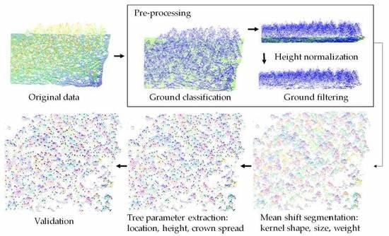
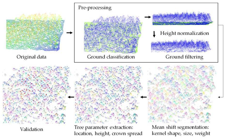
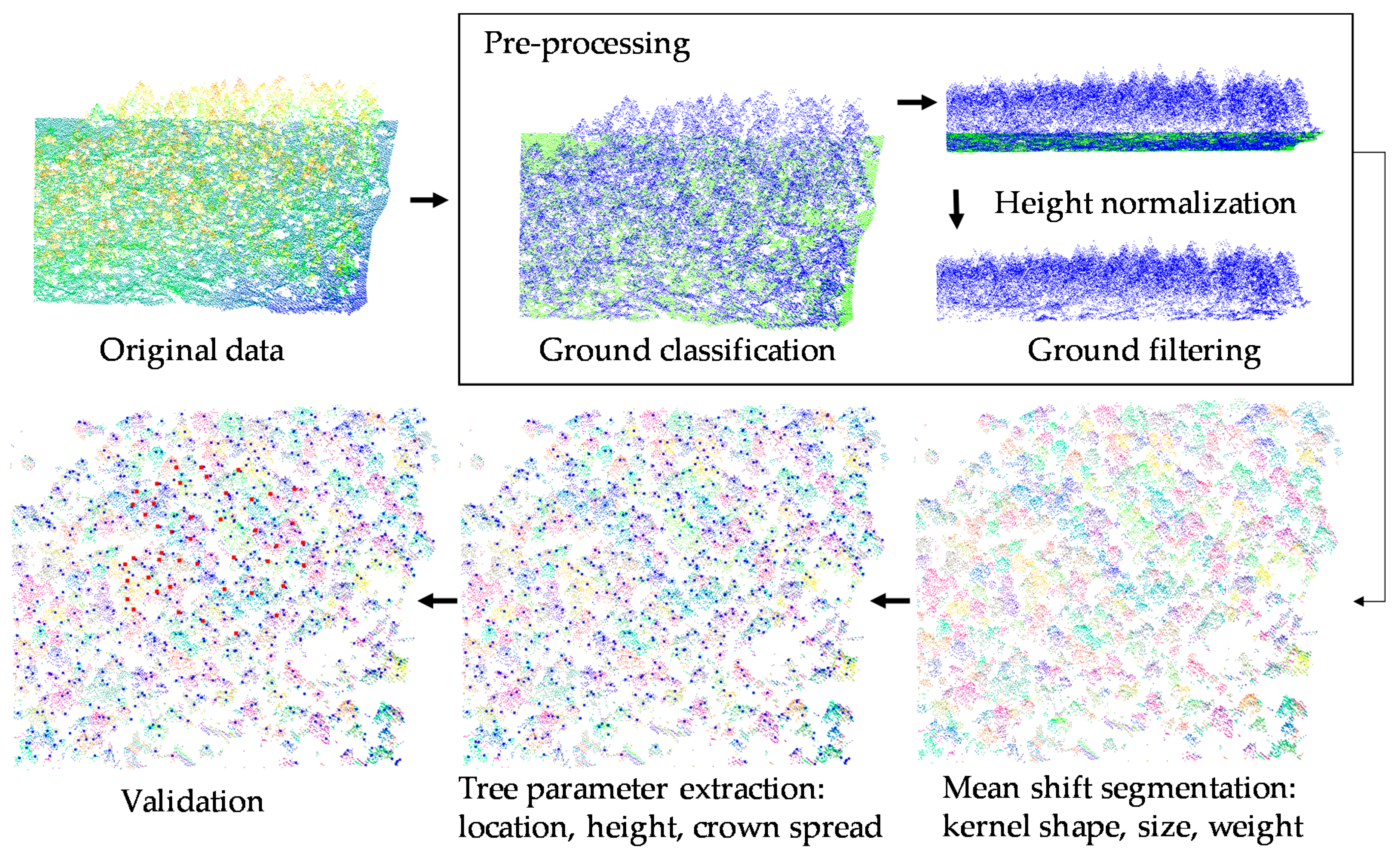
The full workflow of individual forest tree delineation from raw airborne laser scanning data is presented in Figure 1. First, the original point cloud is pre-processed to prepare for the segmentation. Ground points are classified, then the aboveground points are normalized to avoid influence from terrain relief during the segmentation step. In addition, points below 1 m are considered as noise, and thus filtered out. Next, a point-based segmentation method, mean shift, is used to segment the whole point cloud into individual trees. This paper will focus on the assessment of tree segmentation using mean shift, which is an important step that affects the following tree parameter extraction. Other representative methods, such as marker-controlled watershed segmentation [15], are also implemented for comparison. Then for each segment, tree parameters are extracted, such as the location (x, y), height (h), longest crown spread (l) and longest crown cross-spread (l’). Finally, the extractions are validated against field measurements so that the accuracies of the variants of the mean shift algorithm are evaluated.

3.1. Test Data

Three types of plots were used in this study to test the tree segmentation methods: a) A synthetically generated mixed-deciduous woodland, b) a monoculture coniferous stand, and c) two forest plots with a mixture of coniferous and deciduous species.

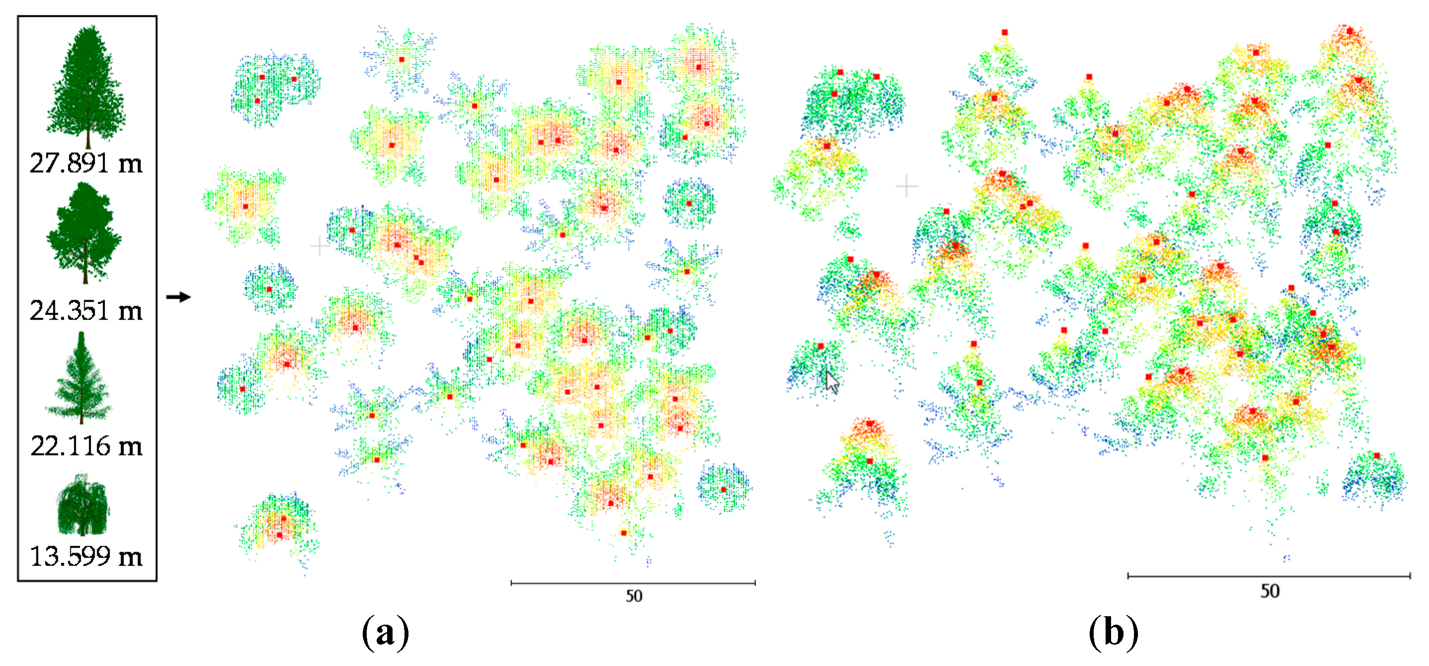
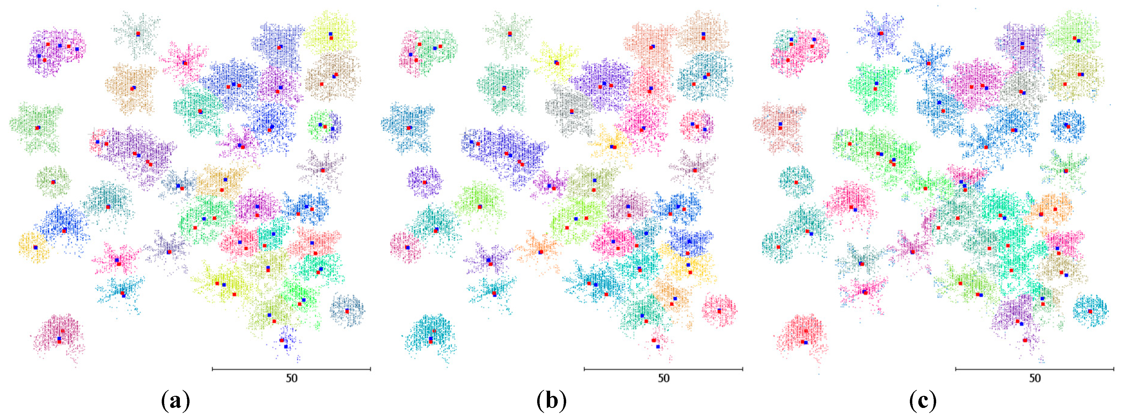
The synthetic dataset (Figure 2) was simulated by the open-source software HELIOS [45]. Main advantages of using synthetic data include: a) Accurate knowledge on the tree locations and crown parameters, and b) control over the number and species of trees. Four species, black tupelo (Nyssa sylvatica Marshall), sassafras (Sassafras albidum), tamarack (Larix laricina (Du Roi) K.Koch), and weeping willow (Salix babylonica L.), were fed into the RIEGL LMS-Q780 simulator to simulate fifty trees randomly located on a 100 m by 100 m square (one hectare). Their heights are 27.891 m, 24.351 m, 22.116 m, and 13.599 m, respectively.

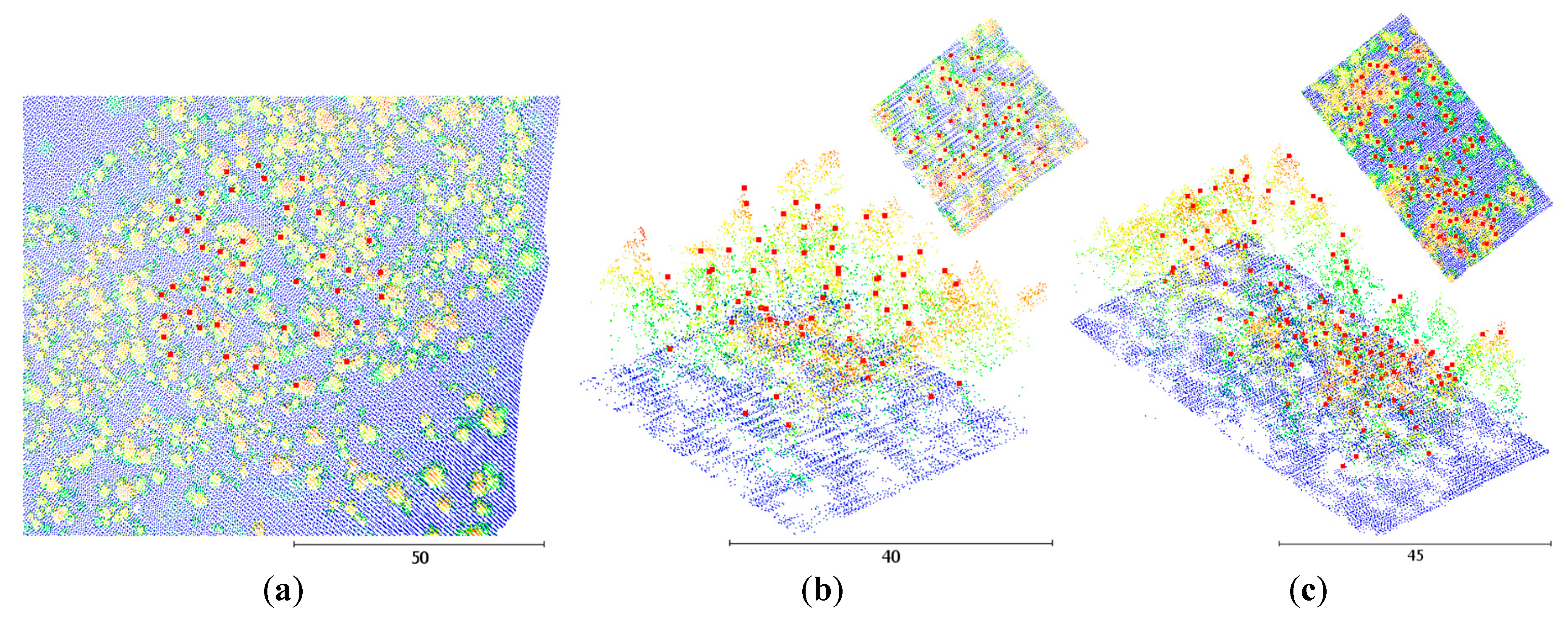
Apart from the synthetic data, an airborne laser scanning (ALS) dataset (8.4 points per m²) of a monoculture plantation stand located in the Queen Elizabeth Forest Park (Aberfoyle, UK) is used for the experiment (Figure 3a). The data were collected by the UK Natural Environment Research Council Airborne Research Facility using the Leica ALS50 Scanner in August 2014. The plot was planted in year 1965, and was composed of lodgepole pine (Pinus contorta Dougl.). Tree parameters, including locations and heights of 45 trees, were surveyed during the field campaign. Tree locations were measured by total station at the bottoms of trees, whilst heights were measured using a vertex hypsometer [46]. The average recorded tree height was 16.18 m, with a standard deviation of 2.12 m. Note that the whole plot contains much more trees, but only this subset covering different tree sizes and densities was measured for validation. Ideally, given a valid tree delineation approach, only a small plot needs to be ground measured to validate the approach and to choose parameters or configurations, which will then be applied to the whole area without further parameter tuning.

The final data of two plots (Plots B1 Figure 3b and B2 Figure 3c, approx. 8 points per m² ) were taken from an international benchmark [22]. They both have a mixture of species, including Norway spruce (Picea abies L.), Scots pine (Pinus sylvestris L.), Downy birch (Betula sp. L.), and Aspen (Populus tremula L.). Plot B1 is predominantly composed of Norway spruce (80%), and the average tree height is 16.8 m with a standard deviation of 6.4 m. Plot B2 has around 55% Norway spruce, and the average tree height is 16.1 m with a standard deviation of 7.31 m. Both plots have multiple crown layers, i.e., dominant, co-dominant, intermediate, and suppressed. The ALS data were collected in June 2004 using an Optech 2033 airborne scanner. Field measurements were collected with a terrestrial laser scanner (TLS), Faro LS880HE. The locations and heights of trees were manually measured from the TLS data.

3.2. Methods

3.2.1. Pre-processing

The Z coordinates of points on trees also contains the elevation of terrain, which can affect the segmentation when the parameters are relevant to the tree height. A common procedure is to normalize the elevation with respect to the ground. Ground classification from airborne light detection and ranging (lidar) data is a well-studied topic [47], and there are both proprietary and free and open-source software available for ground filtering. Lastools (https://rapidlasso.com/lastools/) is adopted here to identify ground points, which are used to normalize other points, so that tree bases are at zero height, and the Z coordinate corresponds to the tree height. After ground filtering, extra points can be observed at ground level, resulting from understory vegetation, e.g., grass or small bushes. As these are not of interest and can affect the segmentation, a 1 m buffer is applied to filter out these points, as suggested by Wang et al. [22]. This height buffer can vary depending on the vertical structure of studied forests. A bigger buffer might be more appropriate if the understory vegetation is higher [28]. The remaining points are considered to be on trees of interest, and will be segmented.

3.2.2. Mean Shift Segmentation

Mean shift has been widely used for image clustering in feature space, which can be multi-dimensional. This section will explain the different adaptations of mean shift for 3D point cloud segmentation. Given a lidar data of n points ${\mathrm{x}}_{\mathrm{i}}$, i = 1,…,n in a 3D space, the mean shift vector can be derived as the gradient of a multivariate kernel density estimator as follows:

$${\mathrm{v}}_{\mathrm{h}}\left(\mathrm{x}\right)=\frac{{{\displaystyle \sum }}_{\mathrm{i}=1}^{\mathrm{n}}{\mathrm{x}}_{\mathrm{i}}\mathrm{g}\left({\Vert \frac{{\mathrm{x}-\mathrm{x}}_{\mathrm{i}}}{\mathrm{h}}\Vert }^2\right)}{{{\displaystyle \sum }}_{\mathrm{i}=1}^{\mathrm{n}}\mathrm{g}\left({\Vert \frac{{\mathrm{x}-\mathrm{x}}_{\mathrm{i}}}{\mathrm{h}}\Vert }^2\right)}-\mathrm{x}$$

(1)

in which $\mathrm{g}(-)$ defines the kernel profile, and h is the bandwidth parameter that determines the size of the kernel. The vector ${\mathrm{v}}_{\mathrm{h}}\left(\mathrm{x}\right)$ is the difference between weighted mean, using the kernel for weights, and point x, the center of the kernel, and is pointing toward the direction of the maximum increase in the density, so that the modes of density can be reached iteratively by translating the kernel (window) by the vector. [30,31] can be referred to for more details. The algorithm has been adapted to a best fit for tree segmentation in terms of kernel shape, size and weight.

Kernel shape: the simplest kernel shape in 3D is a sphere [42], and it is adapted to different shapes to better segment trees, such as a Cylinder [24]. The Pollock model has also been used as the kernel since the model represents the crown shape which can be adjusted by an extra parameter [27].

The model is defined as follows:

$$\mathrm{F}\left(\mathrm{x}\right)={\frac{\mathrm{Z}}{{\mathrm{b}}^{\mathrm{m}}}}^{\mathrm{m}}+\frac{\sqrt{{{(\mathrm{X}}^2{+\mathrm{Y}}^2)}^{\mathrm{m}}}}{{\mathrm{a}}^{\mathrm{m}}}=1$$

(2)

in which x = (X, Y, Z) with respect to the model center, a is the radius of the crown circle in the XY-plane, b is the radius along the Z-axis and m is the crown shape parameter. When m = 1, the model is a cone, and it becomes an ellipsoid as m increases to 2. These three kernel shapes, sphere, cylinder, and Pollock model, will be tested to determine their effects on tree segmentation.

Kernel size: it has been shown that different kernel sizes can be used to segment trees of different sizes and at different layers of the canopy [24], but the settings of the kernel size are mostly trial and error based. Both the Cylinder and Pollock model kernels have two bandwidth/size parameters (a, b) along the horizontal and vertical axes, respectively. Most commonly, the ratio between the two bandwidth parameters b/a is kept fixed during the shifting process, and only one is tuned. Another approach is to adapt the kernel size to the height of trees under the assumption that taller trees will favor a larger kernel, whereas shorter and smaller trees will favor a smaller kernel. This approach is known as continuous adaptive mean shift (Camshift) [27]. In the tests, the kernel size (bandwidth) is tested in two regards, namely, (1) the effects of horizontal bandwidth (a $\in \left[2,3,4,5,6,7,8,9\right])$, and the ratio between the two bandwidth parameters (b/a $\in \left[1,1.5,2,2.5,3\right])$, and (2) whether the kernel is continuously adaptive to the height of the tree (Y or N).

Kernel weight: in addition to the shape of the kernel, different weighting strategies can be applied to the kernel, including weight in the XY-plane, weight in Z, or simply a flat kernel without any weight. Horizontal kernel weights, such as a Gaussian function [24], will put more weight on the center points, meaning the kernel tends to move around less, which will result in more isolated points as standalone clusters. Vertical kernel weights, such as weighting on higher points in the kernel, will lead the kernel to move upwards to converge at the top of a tree [28]. The combination of vertical weight in height $\frac{{\mathrm{Z}-\mathrm{Z}}_{\min }}{{\mathrm{Z}}_{\max }{-\mathrm{Z}}_{\min }}$ and horizontal Gaussian weight for the Pollock kernel can be expressed as follows:

$$\mathrm{g}\left({\Vert \frac{{\mathrm{x}-\mathrm{x}}_{\mathrm{i}}}{\mathrm{h}}\Vert }^2\right)=\{\begin{array}{l}\frac{{\mathrm{Z}-\mathrm{Z}}_{\min }}{{\mathrm{Z}}_{\max }{-\mathrm{Z}}_{\min }}{\mathrm{e}}^{-\mathsf{\lambda }{\Vert \frac{{\mathrm{x}-\mathrm{x}}_{\mathrm{i}}}{\mathrm{h}}\Vert }^2},\mathrm{if}\mathrm{F}\left(\mathrm{x}\right)\le 1\\ 0,\mathrm{otherwise}\end{array}$$

(3)

where $\mathsf{\lambda }$ is set to 0.5 for normal distribution weight in XY, and 0 for weight only in height. Since the dominant direction of a tree is along the vertical axis, weighting in height should facilitate the separation of trees horizontally. Therefore, it will be compared with the Gaussian weight and a flat kernel (no weight) to test its effect on segmentation.

Apart from the kernel configurations, when implementing the mean shift algorithm for segmentation, one rigid but time-consuming practice is to compute the shift for every single point. Another practice is to randomly select seed points to compute the shift. All other points that are covered by the kernel during the shifting process will be assigned the same mode/cluster as the seed points. These two implementations will also be tested for speed and accuracy assessment.

3.2.3. Other Segmentation Methods

A canopy height model (CHM)-based method, marker-controlled watershed [15], was implemented to have an independent reference of the mean shift’s performance. Watershed is also a classical image segmentation method as mean shift. A typical procedure of watershed segmentation of a CHM image is first detecting local maxima in the image, and then segmenting the image by watershed transform. However, the local maxima can be erroneous. To improve the detection, an allometric function of tree height and crown size was introduced to adapt the search window to detect canopy maxima, which were then smoothed by a Gaussian filter. The refined tree tops were used as markers to control the watershed segmentation. Parameters, including search radius and merge radius, as implemented by [48], were fine-tuned for each dataset to produce the best results.

A more recent method from Dalponte et al. [49] was also implemented for comparison. Instead of using watershed, a moving window is used to locate local maxima, which then serve as the ‘initial region’ for region growing, considering the vertical height difference of neighboring pixels. The final regions are approximated by convex hulls, and are treated as tree crowns. In addition, the point-based method proposed for the benchmark data in [22] are tested for further comparison. The point clouds are first voxelized, and some structure elements are proposed for tree top detection, which are constrained by certain rules based on tree morphological characteristics.

3.2.4. Tree Crown Parameter Extraction

Four tree crown parameters (location, height, longest crown spread and longest crown cross-spread) are extracted for the segmented trees following each of the investigated processing variants. The height can be simply taken from the highest point [26]. Tree crown locations will be extracted from the segmented points to evaluate the segmentation step.

There are two main strategies to identify tree crown locations. The first is simply taking the location of the highest point as the location of a tree, which is based on the assumption that the top of the tree is where the tree is located. This is generally true when a tree has a clear peak and is straight upright. The second strategy is to fit a geometric shape to the points on the crown, either in 2D or 3D, which is supposed to be more robust to outliers. To identify the crown location and spreads, the crown base was firstly determined by computing a convex hull around all the tree points in 2D. The average height of the points on the convex hull can be considered as the crown height [27]. Then the crown location, longest spread and longest cross-spread can be determined by fitting an ellipse to these points, where the ellipse center is the crown location, and the two semi-axes represent the two crown spreads. These two strategies will be assessed in this paper to investigate the effects of crown parameter extraction on segmentation validation.

3.3. Validation and Assessment Criteira

In practice, the segmentation is normally validated by checking the locations of segmented trees. That is why the influence of the tree localization method is also investigated. In addition to horizontal locations, the heights of trees can be affected by segmentation, especially when the tree canopy is multistoried or the segmentation method is in 3D. Hence, tree tops (composed of locations and heights) extracted from segmented tree crowns were compared with ground measurements. Even though the segmentation is processed at point-level, the validation is conducted at object-level.

To determine if a tree is oversegmented or undersegmented, the criteria proposed by [22] is followed. In general, if there is only one segmented tree top within a certain range (e.g., 2 m) in 3D from a ground measured tree top, this segment is considered correct (noted as a match). If there is more than one segment in this range or no segment, then the tree is either oversegmented or undersegmented. When all the tested trees have ground truth, such as in the simulated data, the precision, recall and F₁-score can then be calculated as follows:

$$\mathrm{Precision}=\frac{\mathrm{TP}}{\mathrm{TP}+\mathrm{FP}};\mathrm{Recall}=\frac{\mathrm{TP}}{\mathrm{TP}+\mathrm{FN}};{\mathrm{F}}_1=2\frac{\mathrm{Precision}·\mathrm{Recall}}{\mathrm{Precision}+\mathrm{Recall}}$$

(4)

in which TP (True Positive) is the number of matches, FP (False Positive) is the number of oversegmentations inside or outside of the assessment range, FN (False Negative) is the number of undersegmentations.

The horizontal position accuracy and height accuracy are assessed by the root mean square error (RMSE) calculated from the horizontal and vertical distances, respectively, between the detected tree tops and ground measurements.

4. Experiments and Results

4.1. Results of Simulated Data

Extensive experiments were carried out to test the different configurations and parameters of the mean shift approach. As there are many possible combinations of parameter settings, the ones generating better results are reported. The segmentation results of the simulated data are presented in

Table 2. Tree segmentation results of the simulated data using mean shift under various settings. Three kernel shapes are tested: Sphere, Cylinder, and Pollock model, each of which is set to achieve the best result by changing the horizontal bandwidth a, vertical bandwidth ratio b/a, weight in XY, Z or None, adaptiveness (Y or N). Higher results of match, oversegmentation, undersegmentation, precision and F₁-score, are listed. The highest F₁-score for each kernel is highlighted in bold font.

Shape	Band a	Ratio b/a	Weight	Adapt	Match	Over Segment	Under Segment	Precision	F1
Sphere1	3	1	N	Y	0.74	0	0.26	0.1063	0.1859
Sphere2	5	1	N	N	0.76	0	0.24	0.3486	0.4780
Sphere3	7	1	Z	N	0.4	0	0.6	0.5556	0.4651
Cylinder1	4	2	Z	N	0.6	0	0.4	0.6667	0.6316
Cylinder2	2	2	N	N	0.5	0	0.5	0.5682	0.5319
Cylinder3	4	2.5	Z	N	0.6	0	0.4	0.6977	0.6452
Cylinder4	4	1.5	Z	N	0.56	0	0.44	0.6087	0.5833
Pollock1	4	2	N	Y	0.6	0	0.4	0.2804	0.3822
Pollock2	4	2	N	N	0.56	0	0.44	0.6364	0.5957
Pollock3	4	2	Z	N	0.62	0	0.38	0.7381	0.6739
Pollock4	4	2.5	Z	N	0.66	0	0.34	0.7857	0.7174
Pollock5	4	1.5	Y	N	0.62	0	0.38	0.775	0.6889

. The final F₁-scores of sphere kernels are generally lower than the other two kernel shapes, Cylinder and Pollock. The best results from these two kernels are both under the configuration that b/a = 2.5, weighted in height, kernel is not adaptive, bandwidth a = 4. In general, the Pollock model kernels produced better results in terms of both match (recall) and precision, leading to a higher F₁-score. According to the tests, the best performing Pollock model crown parameter was 1.5, regardless the settings of other parameters, which meant that this parameter needed only to be tested once.

The kernels that performed the best, Cylinder3 and Pollock4, were taken to extract tree crown parameters, under the conditions of whether or not the crown is localized by an ellipse. In addition, crown parameters extracted from the segments generated by other compared methods were presented for comparison. The results are illustrated in Figure 4, in which the true tree tops are marked as red points, and the detected tree tops are in blue. It can be seen that for the majority of the trees, detected tree tops can be found nearby, using both Cylinder kernel (Figure 4a) and Pollock kernel (Figure 4b). However, there are few trees where no nearby tree tops are detected. The main reason is that the simulated trees are randomly located, in which case the gaps between trees can be much smaller than in real tree plots. Tree crowns are intertwined, hence they are difficult to separate. The watershed method yielded much worse results (Figure 4c) as trees located in close proximity were clumped together. Higher match rates (recalls) can be obtained when the kernels and searching radius are set to be smaller for both methods, but this will result in higher numbers of false detections, and thus reduce the Precision and final F₁-score.

The tree crown parameter extraction results are presented in

Table 3. Tree top detection results of the simulated data. The best Cylinder and Pollock kernel settings are tested to extract crown locations, using either ellipse centers (Center) or top points (Top), compared with watershed (Mk+WS), region growing (RegGrow) and voxel-based ruling (Vox+Rule) methods. The best results are highlighted in bold. The accuracies of location, height and spreads of detected tree crowns are shown by RMSEs respectively.

Shape	Crown	Match	Precision	F1-Score	RMSE_xy	RMSE_h	RMSE_l	RMSE_l′
Cylinder3	Centre	0.6	0.6977	0.6452	1.2098	0.6116	1.0225	1.9072
Cylinder3	Top	0.7	0.814	0.7527	1.2415	0.4287	1.2428	2.137
Pollock4	Centre	0.66	0.7857	0.7174	1.3849	0.5995	1.0156	1.9044
Pollock4	Top	0.72	0.8571	0.7826	1.2582	0.4336	1.1704	2.1496
Mk+WS	-	0.64	0.9697	0.7711	1.2488	0.5236	1.8598	-
RegGrow	-	0.8	1	0.8889	1.2256	0.4237	2.0324	-
Vox+Rule	-	0.76	0.6333	0.6909	0.9832	0.441	1.9807	-

. The highest match rate and precision of mean shift are achieved when locating the crown by the top point (not the ellipse center from crown fitting) using the Pollok kernel. There are noticeable differences between crown localization results, with locations by the highest point being higher. This is due to the fact that simulated tree models are perfectly upright, so the highest point is where the true tree top is. The variance of the RMSE of tree locations (RMSE_xy) is rather small, but the RMSE of tree height (RMSE_h), when located by the fitted crown center, is greater compared to that by the highest point, whereas the RMSEs of crown spreads (RMSE_l and RMSE_l’) are smaller. It means those extra matched trees have precise tree height estimations, but less precise crown spreads. The compared region growing method shows the best precision and recall (match), hence the highest overall F₁-score. The differences in location and height are of a similar magnitude, but the crown spread is much worse, as it only approximates the average crown diameter, which is different from the longest crown spread.

4.2. Results of Aberfoyle Forest

The results of tree segmentation of the Aberfoyle forest is presented in

Table 4. Tree segmentation results of the Aberfoyle forest using mean shift under various settings.

Shape.	Band a	Ratio b/a	Weight	Adapt	Match	Over Segment	Under Segment
Sphere1	7	1	N	Y	0.8000	0.1111	0.0889
Sphere2	2	1	N	N	0.8000	0.1556	0.0444
Sphere3	2	1	Z	N	0.8000	0.1556	0.0444
Cylinder1	6	2	N	Y	0.8222	0.0444	0.1333
Cylinder2	7	2	Z	Y	0.8222	0.0444	0.1333
Cylinder3	2	2	N	N	0.7333	0.0889	0.1778
Cylinder4	2	2	Z	N	0.6667	0.1111	0.2222
Pollock1	6	2	N	Y	0.8222	0.0222	0.1556
Pollock2	7	2	Z	Y	0.8222	0.0222	0.1556
Pollock3	2	2	N	N	0.7556	0	0.2444
Pollock4	2	2	Z	N	0.7111	0.0444	0.2444

. Note that the ground measured trees do not cover all the trees in the data, only the match rates (recall) can be determined. Therefore, no precision and F₁-Score is given. The precision is related to false detections, which can reflect oversegmentation. The best match rates were achieved by both Cylinder and Pollock kernels. The Sphere kernel produced slightly lower match rates, but the undersegmentation rates were also lower. The Cylinder and Pollock kernels both produced similar results under settings where the kernel size was adaptive to the height, regardless of weighting on the height or not, which is different from the simulated data. So the weight is not very influential for this specific data, which might be due to the less accurate ground measurements. Notice the bandwidth values are also different from what we had with the simulated data, so the best settings for each dataset should be tested.

Similarly, the best performing Cylinder and Pollock kernels were used to extract the crown parameters. The match rates of Cylinder and Pollock kernels are quite similar, but the Cylinder kernel (Figure 5a) produced many more trees than the Pollock kernel (Figure 5b). Some of the detected points are too close to each other to be individual trees, caused by widespread branching and scattered points. The watershed method (Figure 5c) yielded less trees; it can be seen that a number of tree tops were not detected.

Quantitatively, as shown in

Table 5. Tree crown detection results of the Aberfoyle forest. The best Cylinder and Pollock kernel settings are tested to extract crown locations using either ellipse centers (Center) or top points (Top), compared with watershed (Mk+WS), region growing (RegGrow) and voxel-based ruling (Vox+Rule) methods. The best results are highlighted in bold. The accuracies of location, height and crown spreads of detected tree tops are shown by RMSEs compared to the ground truth respectively.

Shape	Crown	Match	Over Segment	Under Segment	RMSE_xy	RMSE_h	RMSE_l	RMSE_l′
Cylinder1	Center	0.8222	0.0444	0.1333	1.27	0.837	1.1406	1.0332
Cylinder1	Top	0.7778	0.0889	0.1333	1.3389	0.9926	1.1304	1.057
Pollock1	Center	0.8222	0.0222	0.1556	1.1845	0.8863	0.9069	0.9093
Pollock1	Top	0.7111	0.0889	0.2	1.2645	0.9304	0.9545	0.9169
Mk+WS	-	0.6889	0.0667	0.2444	1.2276	0.9599	1.0969	-
RegGrow	-	0.7333	0.0444	0.2222	1.3047	0.9293	1.2549	-
Vox+Rule	-	0.7778	0.0667	0.1556	1.043	0.9511	3.1363	-

, the highest match rates were achieved by mean shift when the crown was located by the fitted ellipse center for both Cylinder and Pollock kernels, which is contradictory to the simulated data. As explained for the simulated data, where trees are single layered, perfectly straight, and there is less noise, the highest points do better represent the tree tops. For real tree plots, these conditions do not hold, so the crown fitting gives better results. It is worth noting that the ground truth is measured at tree bottoms, but real trees normally have certain degrees of inclination, hence the assessment of crown locations can be affected. The oversegmentation and undersegmentation rates are also lower when the crown is centered. Among the mean shift models, the smallest RMSE of tree locations (RMSE_xy) was from the Pollock kernel when the crown was centered, which also produced a smaller RMSE of tree height (RMSE_h). The same applied to the Cylinder kernel. Compared to other methods, the lowest match rate, reflected in Figure 5c, were obtained from the watershed method. In addition, the Pollock kernel generates the lowest RMSEs of crown spreads (RMSE_l and RMSE_l’), compared to the Cylinder kernel and the compared methods.

4.3. Results of Benchmark Data

The segmentation results for the two benchmark plots (B1 and B2 in [22]), are presented in

Table 6. Tree segmentation results of the benchmark plots using mean shift under various settings.

Plot	Shape	Band a	Ratio b/a	Weight	Adapt	Match	Over Segment	Under Segment
B1	Sphere1	7	1	N	Y	0.8393	0.0536	0.1071
	Sphere2	2	1	N	N	0.7857	0.1786	0.0357
	Sphere3	2	1	Z	N	0.8214	0.125	0.0536
	Cylinder1	7	2	N	Y	0.8393	0.0536	0.1071
	Cylinder2	7	2	Z	Y	0.8393	0.0714	0.0893
	Cylinder3	2	2	N	N	0.7679	0.0893	0.1429
	Cylinder4	2	2	Z	N	0.7679	0.0179	0.2143
	Pollock1	6	2	N	Y	0.8214	0.0357	0.1429
	Pollock2	7	2	Z	Y	0.8036	0.0714	0.125
	Pollock3	2	2	N	N	0.8571	0.0714	0.0714
	Pollock4	2	2	Z	N	0.875	0.0357	0.0893
B2	Sphere1	8	1	N	Y	0.6637	0.1327	0.2035
	Sphere2	2	1	N	N	0.7788	0.1858	0.0354
	Sphere3	2	1	Z	N	0.8142	0.1593	0.0265
	Cylinder1	8	2	N	Y	0.7611	0.1239	0.115
	Cylinder2	9	2	Z	Y	0.7345	0.1416	0.1239
	Cylinder3	2	2	N	N	0.7699	0.115	0.115
	Cylinder4	2	2	Z	N	0.708	0.0796	0.2124
	Pollock1	9	2	N	Y	0.7345	0.1504	0.115
	Pollock2	9	2	Y	Y	0.7168	0.1681	0.115
	Pollock3	2	2	N	N	0.8142	0.0973	0.0885
	Pollock4	2	2	Y	N	0.8053	0.0885	0.1062

. As the ground truth did not cover all trees in the plots, only the match rates (recall) could be determined. Therefore, no precision and F₁-Score are provided.

For plot B1, the Sphere kernel produced similar match results to the Cylinder kernel when the kernels were adaptive. However, they were both outperformed by the Pollock kernel when the kernel was set to be fixed. For plot B2, the Sphere kernel generated as good match rate as the Pollock kernel, outperforming the Cylinder kernel. The Pollock kernel performed the best for both plots when it was non-adaptive (fixed), such as for the simulated data. Notice that the bandwidth values which generate better results for the two plots are slightly different. Nevertheless, the Pollock kernels that performed the best had the same bandwidth, ratio, and adaptiveness settings. Weighting in Z has an inconsistent impact on the results, as both increases and decreases in match rates are observed compared to no weighting. The Pollock model crown parameter was empirically set to 2 for both plots. This means that the same parameter settings can be applied to both plots, which demonstrates the applicability of the parameter settings to a larger area out of its own plot.

Figure 6 depicts the segmentation results and detected tree tops (blue points) alongside the ground truth (red points). The mean shift method with both Cylinder and Pollock kernels was able to detect tree tops at different layers. The Pollock kernel detected more tree tops than the Cylinder kernel, and had higher match rates for both plots, while maintaining low oversegmentation rates. The watershed method was able to detect some of the dominant and about half of the co-dominant trees, but not intermediate or suppressed trees. It also showed a tendency to under detect trees on the edge of the data. The final detected number of trees was even lower than the ground truth which is a subset of the trees.

The crown locations and heights were compared with ground truth under the two localization strategies to demonstrate the influence on tree segmentation assessment. The final segmentation and validation results are presented in

Table 7. Tree top detection results for the benchmark plots. The best kernel settings are tested to extract tree crowns using either ellipse centers (Center) or top points (Top), compared with watershed (Mk+WS) and region growing (RegGrow) methods. The best results are highlighted in bold. The accuracies of locations and heights of detected tree tops are shown by root mean square errors compared to the ground truth (RMSE_xy, RMSE_h), respectively.

Plot	Shape	Crown	Match	Over Segment	Under Segment	RMSE_xy	RMSE_h
B1	Cylinder1	Center	0.8393	0.0536	0.1071	1.0824	0.8175
	Cylinder1	Top	0.7679	0.0536	0.1786	0.9503	0.7907
	Pollock4	Center	0.875	0.0357	0.0893	0.9639	0.952
	Pollock4	Top	0.8036	0.0536	0.1429	0.9665	0.9338
	Mk+WS	-	0.5893	0.0357	0.375	0.9731	1.8755
	RegGrow	-	0.6607	0.0714	0.2679	1.2175	2.2072
B2	Sphere3	Center	0.8142	0.1593	0.0265	1.0114	0.7787
	Sphere3	Top	0.7788	0.1593	0.0619	1.0429	0.7547
	Pollock3	Center	0.8142	0.0973	0.0885	1.1278	1.0253
	Pollock3	Top	0.7611	0.0973	0.1416	1.1125	0.9702
	Mk+WS	-	0.5398	0.0619	0.3982	1.8795	0.7606
	RegGrow	-	0.6018	0.0442	0.354	1.3739	1.5071

. The crown centered by fitted ellipse improved the crown matching rate for both kernels in both plots. The match rates of the watershed and region growing methods were rather low, which was due to the fact that the plots were multi-layered, and that the raster-based method is less capable of capturing the lower layers. The RMSEs in locations (RMSE_xy) and height (RMSE_h) of the mean shift method varied slightly, whether the crown was localized or not, and they are generally better than that of the two raster-based methods.

More individual tree delineation methods were tested on the benchmark data as presented in [22]. The comparisons with other methods are shown in

Table 8. Mean shift (MS) tree detection results of the benchmark plots compared to methods in [22].

Plot	Class	FGI	IGN	SLU1	SLU2	UZH	MS
	All	0.8491	0.4941	0.6911	0.6911	0.7784	0.875
	Dominant	0.96	0.65	0.93	0.93	0.96	1
B1	Codominant	0.88	0.55	0.66	0.66	0.88	0.8889
	Intermediate	0.66	0.16	0.25	0.25	0.33	0.75
	Suppressed	0.33	0	0	0	0.33	0
	All	0.8864	0.4596	0.6936	0.7171	0.8027	0.8142
	Dominant	1	0.7	0.92	0.93	0.98	0.9091
B2	Codominant	0.88	0.42	0.73	0.73	0.83	0.7667
	Intermediate	0.91	0.06	0.42	0.5	0.63	0.5714
	Suppressed	0.43	0	0	0.07	0.22	0.7857

. The mean shift performed the best in plot B1, but was outperformed by the FGI method in plot B2.

4.4. Computing Costs

The computing time of a single plot is not significant, but for a larger study area with higher lidar point density, the computing time can be a factor to consider when choosing the segmentation method. The Aberfoyle plot is taken to test the speed of segmentation, as it has the largest coverage (106 m by 88 m), with more trees and higher point density. The computing costs of the mean shift with fixed and adaptive kernels for iterating, both over each point and random seed points, are recorded. In addition, the computing times of the watershed and region growing methods are also recorded for comparison.

Table 9. Computing times in seconds (s) of mean shift when the kernel is fixed (MS_fix) or adaptive (MS_adaptive) for random seed points or each point, compared to watershed and region growing.

Settings	MS_fix	MS_adaptive	Mk+WS	RegGrow
Random	10.15	23.31	0.016	0.97
Each point	80.13	160.62	-	-

shows the computing times of mean shift and watershed running with an Intel Core i7-6700HQ CPU on a 64 bit laptop system in MATLAB R2018a, and of region growing in R. The time doubled when the kernel was set to be adaptive. Also the cost is about eight times higher when the shift is computed for each individual point. There are also slight differences when using different kernel shapes and weightings, but they can be neglected compared to the reported settings. When choosing random seed points, the segmentation results will vary for each run. On average, the matching rate is 5% to 10% lower than that computed on every point. The watershed method, although producing the lowest matching results, is significantly faster than mean shift. The region growing method performed consistently better than watershed, and took slightly longer time, but it was still much faster than mean shift.

5. Discussion

The mean shift algorithm was tested on three different airborne lidar datasets. The settings generating the best results varied slightly across the data. Nevertheless, certain recommendations can be made based on the tests.

The Pollock model as the kernel produced the best results for all three datasets. This proves the assumption that a kernel that ensembles the crown shape will facilitate crown segmentation. Although there is one more parameter to be tuned, i.e., the crown shape, it only needs to be tested once on a subset of data, even if the data are of mixed species. For example, for the benchmark data, the same crown shape (m = 2) was set for both plots in the same forest. The Cylinder kernel also produced good results for all the tested data, similar to those demonstrated in previous studies [26,28]. There are two kernel bandwidth parameters to be tested (a and b), and they can be reduced to one if the ratio (b/a) is pre-defined [24]. The spherical kernel was the simplest, but yielded the worst results apart from the benchmark plot B2. Given the fact that the Cylinder kernel is not much more complex, a first attempt to directly use the Cylinder would be recommended. The Pollock kernel would be preferred for better results with slightly more parameter tuning.

Adapting the kernel to the crown size is considered to be a valid improvement of mean shift. However, whether or not to make the kernel continuously adaptive, for instance to the tree height, is dependent on the data as demonstrated by the results. Considering that the continuous adaptiveness will cost twice the computing time, and not necessarily generate better outcome, a fixed kernel is recommended. This adaptiveness is based on the assumption that taller trees have larger crown sizes, which may not be true for mixed species forests. One possible improvement is to adapt the kernel to the individual tree crown size rather than the height. There have been attempts to extract information of the crown size from either allometric approximations [26] or crown detection [42]. In both cases, the kernel was adapted to the targeted crown sizes generated from extra steps.

The weighting in the vertical direction is proved to be beneficial in some cases but not always. Higher points in the kernel have higher weights, which helps the kernel to move upwards, so that the shift can be converged at the top of the tree. In this paper the weight is normalized to [0, 1], so the highest point has weight 1, and the lowest has weight 0. Other types of weighting strategy can be designed, such as the one in [28]. The weighting in the horizontal plane did not improve the results as assumed, hence was not presented in the tables. The Gaussian function puts more weight on points near the center point, i.e., the mean, and less weight on points near the boundary of the kernel, so that the kernel is less likely to shift if there are not enough points outside of the center area of the kernel. Therefore, weighting in either height or in the XY plane should be further investigated before implementing for each specific data.

Crown localization is assessed because crown tops are used to validate the segmentation results. Crown tops can be simply decided by the highest points of the segmented crowns. But the tree locations can be inaccurate, as real trees are normally not perfectly straight upwards. An alternative approach is to fit the segmented crowns with ellipses and take the ellipse centers as crown locations. The results varied in this regard. The results of the simulated data showed clear advantage when simply using the highest points as tree tops, giving better segmentation results and lower RMSEs, whereas the results of the Aberfoyle data showed the contrary, better segmentation results and lower RMSEs when fitting the crowns with ellipses. This is because the first simulated data are perfectly upright trees with almost symmetric crowns, whereas the second is from a plantation forest where most trees are naturally inclined, and have more diverse crown structures. The benchmark data also showed better segmentation results when fitting the crowns, hence crown fitting for tree top detection is recommended for real forests. The localization accuracy itself can be further assessed when accurate ground truth of crown locations are available, which can be difficult by either field measurements or other sensing techniques [50].

The compared marker-controlled watershed method performed well on the simulated data, with a particularly high precision. Similarly, the raster-based region growing method produced the best results for the simulated data. However, both were outperformed by the two point-based methods. For such a simple and single-layered plot, raster-based methods are expected to have a good performance. However, it clearly struggled with a more natural data, especially with the multi-layered benchmark plots. The advantage is that they are extremely fast, thus are still worth trying for less structurally complicated forests. Even though the focus of the paper is on the thorough assessment of the mean shift method itself, the comparisons with other raster- and point-based methods prove the value of such assessment, as mean shift is able to produce competitive results.

There are other possible improvements of mean shift segmentation for ITD. For example, the Pollock model crown parameter can be adaptive from prior knowledge, or classification from other data sources. Raster-based methods can be combined with mean shift to approximately estimate the crown size, which can then feed into the kernel. Moreover, a hierarchical approach can be adopted, similar to [28], where the data is segmented by mean shift in two rounds. The first round segments the original data into plausible individual trees. A pre-trained classifier is then used to detect the oversegmented and undersegmented trees, which are refined by a second round of mean shift segmentation with appropriate parameter settings derived from the classification. As these approaches require extra steps other than the mean shift algorithm, they are considered to be out of the scope of the paper, which is focusing on the assessment of the method itself.

6. Conclusions

This paper conducted a thorough performance assessment of the mean shift algorithm for individual tree delineation from airborne lidar data. Three main factors considered are kernel shape, kernel size adaptiveness, and kernel weighting. They were assessed in three different datasets, one simulated data, one UK forest data, and one benchmark data from Finland.

The results suggested that the Pollock model used as the mean shift kernel can improve the segmentation, though there are a few parameters that would have to be fine-tuned. On the other hand, the Cylinder kernel, commonly used in other studies, can generate good results while maintaining simplicity. The continuous adaptive strategy works for certain data, but might not be reliable due to the complexity of crown structures, whilst being time consuming. The weighting in height is recommended to be tested for different datasets, whereas horizontal weighting should be undertaken with caution. Finally, the validation results can be affected by the ground truth quality, as real crown positions are difficult to determine from neither ground survey nor other data sources.

The effectiveness of mean shift is proved by comparing with two raster-based methods, marker-controlled watershed and region growing, which performed well on single-layered data, and were extremely fast. Further improvements to the segmentation workflow by introducing additional steps, such as integrating point-based and raster-based methods, will be investigated in future work.

References

1. Thompson, I.; Mackey, B.; McNulty, S.; Mosseler, A. Forest Resilience, Biodiversity, and Climate Change; Secretariat of the Convention on Biological Diversity: Montreal, QC, Canada, 2009; Volume 43, pp. 1–67. [Google Scholar]
2. Franklin, S.E. Remote Sensing for Sustainable Forest Management; CRC Press: Boca Raton, FL, USA, 2001. [Google Scholar]
3. Lim, K.; Treitz, P.; Wulder, M.; St-Onge, B.; Flood, M. LiDAR remote sensing of forest structure. Prog. Phys. Geogr. 2003, 27, 88–106. [Google Scholar] [CrossRef] [Green Version]
4. Qi, W.; Dubayah, R.O. Combining Tandem-X InSAR and simulated GEDI lidar observations for forest structure mapping. Remote Sens. Environ. 2016, 187, 253–266. [Google Scholar] [CrossRef]
5. Koch, B.; Heyder, U.; Weinacker, H. Detection of individual tree crowns in airborne lidar data. Photogramm. Eng. Remote Sens. 2006, 72, 357–363. [Google Scholar] [CrossRef]
6. Wallace, L.; Lucieer, A.; Watson, C.S. Evaluating tree detection and segmentation routines on very high resolution UAV LiDAR data. IEEE Trans. Geosci. Remote Sens. 2014, 52, 7619–7628. [Google Scholar] [CrossRef]
7. Liang, X.; Kukko, A.; Hyyppä, J.; Lehtomäki, M.; Pyörälä, J.; Yu, X.; Kaartinen, H.; Jaakkola, A.; Wang, Y. In-situ measurements from mobile platforms: An emerging approach to address the old challenges associated with forest inventories. ISPRS J. Photogramm. Remote Sens. 2018, 143, 97–107. [Google Scholar] [CrossRef]
8. Liang, X.; Kankare, V.; Hyyppä, J.; Wang, Y.; Kukko, A.; Haggrén, H.; Yu, X.; Kaartinen, H.; Jaakkola, A.; Guan, F.; et al. Terrestrial laser scanning in forest inventories. ISPRS J. Photogramm. Remote Sens. 2016, 115, 63–77. [Google Scholar] [CrossRef]
9. Wehr, A.; Lohr, U. Airborne laser scanning—An introduction and overview. ISPRS J. Photogramm. Remote Sens. 1999, 3, 68–82. [Google Scholar] [CrossRef]
10. Zimble, D.A.; Evans, D.L.; Carlson, G.C.; Parker, R.C.; Grado, S.C.; Gerard, P.D. Characterizing vertical forest structure using small-footprint airborne LiDAR. Remote Sens. Environ. 2003, 3, 171–182. [Google Scholar] [CrossRef]
11. Means, J.E.; Acker, S.A.; Fitt, B.J.; Renslow, M.; Emerson, L.; Hendrix, C.J. Predicting forest stand characteristics with airborne scanning lidar. Photogramm. Eng. Remote Sens. 2000, 66, 1367–1372. [Google Scholar]
12. Zhen, Z.; Quackenbush, L.; Zhang, L. Trends in automatic individual tree crown detection and delineation—Evolution of LiDAR data. Remote Sens. 2016, 8, 333. [Google Scholar] [CrossRef]
13. Næsset, E. Predicting forest stand characteristics with airborne scanning laser using a practical two-stage procedure and field data. Remote Sens. Environ. 2002, 80, 88–99. [Google Scholar] [CrossRef]
14. Lee, H.; Slatton, K.C.; Roth, B.E.; Cropper, W., Jr. Adaptive clustering of airborne LiDAR data to segment individual tree crowns in managed pine forests. Int. J. Remote Sens. 2010, 31, 117–139. [Google Scholar] [CrossRef]
15. Chen, Q.; Baldocchi, D.; Gong, P.; Kelly, M. Isolating individual trees in a savanna woodland using small footprint lidar data. Photogramm. Eng. Remote Sens. 2006, 72, 923–932. [Google Scholar] [CrossRef]
16. Lu, X.; Guo, Q.; Li, W.; Flanagan, J. A bottom-up approach to segment individual deciduous trees using leaf-off lidar point cloud data. ISPRS J. Photogramm. Remote Sens. 2014, 94, 1–12. [Google Scholar] [CrossRef]
17. Eysn, L.; Hollaus, M.; Lindberg, E.; Berger, F.; Monnet, J.-M.; Dalponte, M.; Kobal, M.; Pellegrini, M.; Lingua, E.; Mongus, D.; et al. A benchmark of LiDAR-based single tree detection methods using heterogeneous forest data from the Alpine space. Forests 2015, 6, 1721–1747. [Google Scholar] [CrossRef]
18. Jakubowski, M.; Li, W.; Guo, Q.; Kelly, M. Delineating individual trees from LiDAR data: A comparison of vector-and raster-based segmentation approaches. Remote Sens. 2013, 5, 4163–4186. [Google Scholar] [CrossRef]
19. Bruggisser, M.; Hollaus, M.; Wang, D.; Pfeifer, N. Adaptive Framework for the Delineation of Homogeneous Forest Areas Based on LiDAR Points. Remote Sens. 2019, 11, 189. [Google Scholar] [CrossRef]
20. Li, W.; Guo, Q.; Jakubowski, M.K.; Kelly, M. A new method for segmenting individual trees from the lidar point cloud. Photogramm. Eng. Remote Sens. 2012, 78, 75–84. [Google Scholar] [CrossRef]
21. Hamraz, H.; Contreras, M.A.; Zhang, J. A robust approach for tree segmentation in deciduous forests using small-footprint airborne LiDAR data. Int. J. Appl. Earth Obs. Geoinf. 2016, 52, 532–541. [Google Scholar] [CrossRef] [Green Version]
22. Wang, Y.; Hyyppä, J.; Liang, X.; Kaartinen, H.; Yu, X.; Lindberg, E.; Holmgren, J.; Qin, Y.; Mallet, C.; Ferraz, A.; et al. International Benchmarking of the Individual Tree Detection Methods for Modeling 3-D Canopy Structure for Silviculture and Forest Ecology Using Airborne Laser Scanning. IEEE Trans. Geosci. Remote Sens. 2016, 54, 5011–5027. [Google Scholar] [CrossRef] [Green Version]
23. Strîmbu, V.F.; Strîmbu, B.M. A graph-based segmentation algorithm for tree crown extraction using airborne LiDAR data. ISPRS J. Photogramm. Remote Sens. 2015, 104, 30–43. [Google Scholar] [CrossRef] [Green Version]
24. Ferraz, A.; Bretar, F.; Jacquemoud, S.; Gonçalves, G.; Pereira, L.; Tomé, M.; Soares, P. 3-D mapping of a multi-layered Mediterranean forest using ALS data. Remote Sens. Environ. 2012, 121, 210–223. [Google Scholar] [CrossRef]
25. Mongus, D.; Žalik, B. An efficient approach to 3D single tree-crown delineation in LiDAR data. ISPRS J. Photogramm. Remote Sens. 2015, 108, 219–233. [Google Scholar] [CrossRef]
26. Ferraz, A.; Saatchi, S.; Mallet, C.; Meyer, V. Lidar detection of individual tree size in tropical forests. Remote Sens. Environ. 2016, 183, 318–333. [Google Scholar] [CrossRef]
27. Xiao, W.; Xu, S.; Elberink, S.O.; Vosselman, G. Individual Tree Crown Modeling and Change Detection From Airborne Lidar Data. IEEE J. Sel. Top. Appl. Earth Obs. Remote Sens. 2016, 9, 3467–3477. [Google Scholar] [CrossRef]
28. Dai, W.; Yang, B.; Dong, Z.; Shaker, A. A new method for 3D individual tree extraction using multispectral airborne LiDAR point clouds. ISPRS J. Photogramm. Remote Sens. 2018, 144, 400–411. [Google Scholar] [CrossRef]
29. Fukunaga, K.; Hostetler, L. The estimation of the gradient of a density function, with applications in pattern recognition. IEEE Trans. Inf. Theory 1975, 21, 32–40. [Google Scholar] [CrossRef]
30. Cheng, Y. Mean shift, mode seeking, and clustering. IEEE Trans. Pattern Anal. Mach. Intell. 1995, 17, 790–799. [Google Scholar] [CrossRef]
31. Comaniciu, D.; Meer, P. Mean shift: A robust approach toward feature space analysis. IEEE Trans. Pattern Anal. Mach. Intell. 2002, 24, 603–619. [Google Scholar] [CrossRef]
32. Comaniciu, D.; Ramesh, V.; Meer, P. Real-time tracking of non-rigid objects using mean shift. In Proceedings of the IEEE Conference on Computer Vision and Pattern Recognition, Hilton Head Island, SC, USA, 15 June 2000; pp. 142–149. [Google Scholar]
33. Huang, X.; Zhang, L. An adaptive mean-shift analysis approach for object extraction and classification from urban hyperspectral imagery. IEEE Trans. Geosci. Remote Sens. 2008, 46, 4173–4185. [Google Scholar] [CrossRef]
34. Michel, J.; Youssefi, D.; Grizonnet, M. Stable mean-shift algorithm and its application to the segmentation of arbitrarily large remote sensing images. IEEE Trans. Geosci. Remote Sens. 2015, 53, 952–964. [Google Scholar] [CrossRef]
35. Bo, S.; Ding, L.; Li, H.; Di, F.; Zhu, C. Mean shift-based clustering analysis of multispectral remote sensing imagery. Int. J. Remote Sens. 2009, 30, 817–827. [Google Scholar] [CrossRef]
36. Maschler, J.; Atzberger, C.; Immitzer, M. Individual Tree Crown Segmentation and Classification of 13 Tree Species Using Airborne Hyperspectral Data. Remote Sens. 2018, 10, 1218. [Google Scholar] [CrossRef]
37. Melzer, T. Non-parametric segmentation of ALS point clouds using mean shift. J. Appl. Geod. Jag 2007, 1, 159–170. [Google Scholar] [CrossRef]
38. Yao, W.; Hinz, S.; Stilla, U. Object extraction based on 3d-segmentation of lidar data by combining mean shift with normalized cuts: Two examples from urban areas. In Proceedings of the 2009 Joint Urban Remote Sensing Event, Shanghai, China, 20–22 May 2009; pp. 1–6. [Google Scholar]
39. Lee, I.-C.; Wu, B.; Li, R. Shoreline extraction from the integration of lidar point cloud data and aerial orthophotos using mean-shift segmentation. In Proceedings of the 2009 ASPRS Annual Conference, Baltimore, MD, USA, 9–13 March 2009; Volume 2, pp. 3033–3040. [Google Scholar]
40. Ferraz, A.; Bretar, F.; Jacquemoud, S.; Gonçalves, G.; Pereira, L. 3D segmentation of forest structure using a mean-shift based algorithm. In Proceedings of the 2010 IEEE International Conference on Image Processing, Hong Kong, China, 26–29 September 2010; pp. 1413–1416. [Google Scholar]
41. Yao, W.; Krzystek, P.; Heurich, M. Enhanced detection of 3D individual trees in forested areas using airborne full-waveform LiDAR data by combining normalized cuts with spatial density clustering. ISPRS Ann. Photogramm. Remote Sens. Spat. Inf. Sci. 2013, 1, 349–354. [Google Scholar] [CrossRef]
42. Amiri, N.; Yao, W.; Heurich, M.; Krzystek, P.; Skidmore, A.K. Estimation of regeneration coverage in a temperate forest by 3D segmentation using airborne laser scanning data. Int. J. Appl. Earth Obs. Geoinf. 2016, 52, 252–262. [Google Scholar] [CrossRef]
43. Hu, X.; Chen, W.; Xu, W. Adaptive Mean Shift-Based Identification of Individual Trees Using Airborne LiDAR Data. Remote Sens. 2017, 9, 148. [Google Scholar] [CrossRef]
44. Chen, W.; Hu, X.; Chen, W.; Hong, Y.; Yang, M. Airborne LiDAR remote sensing for individual tree forest inventory using trunk detection-aided mean shift clustering techniques. Remote Sens. 2018, 10, 1078. [Google Scholar] [CrossRef]
45. Bechtold, S.; Höfle, B. HELIOS: A multi-purpose lidar simulation framework for research, planning and training of laser scanning operations with airborne, ground-based mobile and stationary platforms. ISPRS Ann. Photogramm. Remote Sens. Spat. Inf. Sci. 2016, 3. [Google Scholar] [CrossRef]
46. Smigaj, M.; Gaulton, R.; Suárez, J.C.; Barr, S.L. Combined use of spectral and structural characteristics for improved red band needle blight detection in pine plantation stands. For. Ecol. Manag. 2019, 434, 213–223. [Google Scholar] [CrossRef]
47. Meng, X.; Currit, N.; Zhao, K. Ground filtering algorithms for airborne LiDAR data: A review of critical issues. Remote Sens. 2010, 2, 833–860. [Google Scholar] [CrossRef]
48. Parkan, M. Digital Forestry Toolbox for Matlab/Octave. Available online: http://mparkan.github.io/Digital-Forestry-Toolbox/ (accessed on 20 March 2019).
49. Dalponte, M.; Coomes, D.A. Tree-centric mapping of forest carbon density from airborne laser scanning and hyperspectral data. Methods Ecol. Evol. 2016, 7, 1236–1245. [Google Scholar] [CrossRef]
50. Wang, Y.; Lehtomäki, M.; Liang, X.; Pyörälä, J.; Kukko, A.; Jaakkola, A.; Liu, J.; Feng, Z.; Chen, R.; Hyyppä, J. Is field-measured tree height as reliable as believed—A comparison study of tree height estimates from field measurement, airborne laser scanning and terrestrial laser scanning in a boreal forest. ISPRS J. Photogramm. Remote Sens. 2019, 147, 132–145. [Google Scholar] [CrossRef]
Figure 1. The workflow of individual forest tree delineation from airborne light detection and ranging (lidar) data.
Remotesensing 11 01263 g001
Figure 2. Synthetic data simulated by HELIOS (scale in meters). (a) Tree models and simulated data in bird’s eye view, (b) Perspective view. There are 50 trees in total, of four species at different heights. Red points represent tree tops.
Remotesensing 11 01263 g002
Figure 3. Experiment data (scale in meters). (a) A plot of the Aberfoyle forest in Scotland, UK. (b) Plot B1 from an international benchmark. (c) Plot B2 from an international benchmark. Red points represent ground measured tree tops.
Remotesensing 11 01263 g003
Figure 4. Segmentation and tree top detection results of the simulated data from three methods (scale in meters): (a) Mean shift with Cylinder kernel; (b) Mean shift with Pollock kernel; (c) Marker-controlled watershed method. Red points denote true tree tops, and blue ones are detected tops.
Remotesensing 11 01263 g004
Figure 5. Segmentation and tree top detection results of the Aberfoyle forest from three methods (scale in meters): (a) Mean shift with Cylinder kernel; (b) Mean shift with Pollock kernel; (c) Marker controlled watershed method. Red points denote true tree tops, and blue ones are detected tops.
Remotesensing 11 01263 g005
Figure 6. Segmentation and tree top detection results of the benchmark plots (first two rows: plot B1, second two rows: plot B2) from three methods (scale in meters): (a,d) Mean shift with Cylinder kernel; (b,e) Mean shift with Pollock kernel; (c,f) Marker-controlled watershed method. Red points denote true tree tops, and blue ones are detected tops.
Remotesensing 11 01263 g006