SAR ATR of Ground Vehicles Based on ESENet

Abstract

In recent studies, synthetic aperture radar (SAR) automatic target recognition (ATR) algorithms that are based on the convolutional neural network (CNN) have achieved high recognition rates in the moving and stationary target acquisition and recognition (MSTAR) dataset. However, in a SAR ATR task, the feature maps with little information automatically learned by CNN will disturb the classifier. We design a new enhanced squeeze and excitation (enhanced-SE) module to solve this problem, and then propose a new SAR ATR network, i.e., the enhanced squeeze and excitation network (ESENet). When compared to the available CNN structures that are designed for SAR ATR, the ESENet can extract more effective features from SAR images and obtain better generalization performance. In the MSTAR dataset containing pure targets, the proposed method achieves a recognition rate of 97.32% and it exceeds the available CNN-based SAR ATR algorithms. Additionally, it has shown robustness to large depression angle variation, configuration variants, and version variants.

1. Introduction

Synthetic aperture radar (SAR) has played a significant role in surveillance and battlefield reconnaissance, thanks to its all-day, all-weather, and high resolution capability. In recent years, SAR automatic target recognition (ATR) of ground military vehicles has received intensive attention in the radar ATR community. However, SAR images usually have low resolution and they only contain the amplitude information of scattering centers. Thus, it is challenging to identify the targets in SAR images.

The MIT Lincoln Laboratory proposed the standard SAR ATR architecture, which consists of three stages: detection, discrimination, and classification [1]. In the detection stage, simple decision rules are used to find the bright pixels in SAR images and indicate the presence of targets. The output of this stage might include not only targets of interests, but also clutters, because the decision stage is far from perfect. On the following discrimination stage, a discriminator is designed to solve a two-class (target and clutter) classification problem and the probability of false alarm can be significantly reduced [2]. On the final classification stage, a classifier is designed to categorize each output image of the discrimination stage as a specific target type.

On the classification stage, there are three mainstream methods: template matching methods, model-based methods, and machine learning methods. For the template matching methods [3,4], the template database is generated from training samples according to some matching rules and the best match is then found by comparing each test sample to the template database. The common matching rules are the minimum mean square error, the minimum Euclidean distance, and the maximum correlation coefficient, etc. In these template matching methods, the initial SAR images or sub-images cut from initial SAR images are served as templates. However, the SAR images are sensitive to azimuth angle, depression angle, and target structure. When there is large difference between the training and test samples, the recognition performance will severely decrease. Additionally, such methods suffer from severe overfitting [5]. Model-based methods were proposed to solve the above problem [6,7]. In the model-based methods, SAR images are predicted by computer-aided design model and the modeling procedure is usually complicated.

SAR ATR algorithms that are based on machine learning methods can be further divided into two types, i.e., feature-based methods and deep learning methods. Feature-based methods [8,9] require features to be manually extracted from SAR images, while deep learning methods automatically extract features from SAR images. Thus, deep learning methods avoid the designing of feature extractors. As a typical deep learning structure, convolutional neural network (CNN) has been successfully applied in various fields, e.g., SAR image classification [10] and satellite image classification [11]. Particularly, CNN-based methods outperform others in SAR ATR tasks due to its unique characteristics that are suitable for two-dimensional image classification [12].

The MSTAR dataset serves as a benchmark for SAR ATR algorithms evaluation and comparison [13]. However, there is high-correlation between the target type and clutter in the MSTAR dataset, i.e., the SAR images of a specific target type may correspond to the same background clutter. It was demonstrated that, even if the target and shadow regions are removed, a traditional classifier still achieves high recognition accuracy (above 99%) for the remaining clutters [14]. It may be impossible that the target location may change in real world situations, and various background clutters instead of a fixed type should accompany the corresponding SAR image. Therefore, we exclude such correlation by target region segmentation [15] and generate the MSTAR pure target dataset for fair comparison and an evaluation of SAR ATR algorithms.

The key factors in improving the recognition performance of SAR ATR algorithms that are based on CNN include: (i) SAR image preprocessing to extract features more effectively and easily; and, (ii) designing effective network structures that make full use of the extracted features from SAR images.

Ding et al. [16] augmented the training set by image rotation and shifting to alleviate over-fitting for SAR image preprocessing. Chen et al. generated the augmented training set by cropping the initial 128 × 128 MSTAR images to 88 × 88 patches randomly [12]. Wagner enlarged the training set by directly adding distorted SAR images to improve the robustness [17]. Lin et al. cropped the initial MSTAR images to 68 × 68 patches in order to reduce the computation burden of CNN [18] and Shang et al. cropped the initial MSTAR images to 70 × 70 patches [19]. Wang et al. used a despeckling subnetwork to suppress speckle noise before inputting SAR images into a classification network [20].

For the designing of CNN structure for SAR ATR, a traditional CNN structure that consists of convolutional layers, pooling layers and softmax classifier was proposed [16,21,22,23]. Later, Chen et al. designed A-convent, where the number of unknown parameters is greatly reduced by removing the fully-connected layer [12]. Wagner replaced the softmax classifier in the traditional CNN structure by a SVM classifier and achieved high recognition accuracy [17,24]. Lin et al. proposed CHU-Nets, where a convolutional highway unit is inserted into the traditional CNN structure and the classification performance is improved in a limited-labeled training dataset [18]. Shang et al. added an information recorder to CNN to remember and store the spatial features of the samples, and then used spatial similarity information of the recorded features to predict the unknown sample labels [19]. Kechagias-Stamatis et al. fused a convolutional neural network module with a sparse coding module under a decision level scheme, which can adaptively alter the fusion weights that are based on the SAR images [25]. Pei et al. proposed a multiple-view DCNN (m-VDCNN) to extract the features from target images with different azimuth angles [26].

Generally, CNN is a data-driven model and each pixel of the training and test samples directly participates in feature extraction. The correlation between the clutter in the training and test sets cannot be ignored, since input SAR images consist of both target region and clutter region. Additionally, for the available SAR ATR algorithms that are based on CNN, the softmax classifier directly applies the features that were extracted by convolutional layers. However, CNN may automatically learn the useless feature maps, which prevent the classifier from effectively utilizing significant features [27,28]. Therefore, the available SAR ATR algorithms that are based on CNN ignore the negative effects of the feature maps with little information, and the recognition performance may degrade.

We propose a novel SAR ATR algorithm based on CNN to tackle the above-mentioned problems. The main contributions includes: (i) an enhanced Squeeze and Excitation (SE) module is proposed to suppress feature maps with little information in CNN by allocating different weights to feature maps according to the amount of information they contain; and, (ii) a modified CNN structure, i.e., the Enhanced Squeeze and Excitation Net (ESENet) incorporating the enhanced-SE module is proposed. The experimental results on the MSTAR dataset without clutter have shown that the proposed network outperforms the available CNN structures designed for SAR ATR.

The remainder of this paper is organized, as follows. Section 2 introduces the Squeeze and Excitation module. Section 3 introduces a novel SAR ATR method based on the ESENet, and discusses the mechanism of the enhanced-SE module, together with the structure of the ESENet in detail. Section 4 presents the experimental results to validate the effectiveness of the proposed network, and Section 5 concludes the paper.

2. Squeeze and Excitation Module

A typical CNN structure consists of a feature extractor and a classifier. The feature extractor is a multilayer structure that is formed by stacking convolutional layers and pooling layers. The feature maps of different hierarchies are extracted layer by layer, and then feature maps of the last layer are applied by the classifier for target recognition. In a typical feature extractor, the feature maps in the same layer are regarded as having the same importance to the next layer. However, such an assumption is usually violated in practice [29]. Figure 1 shows 16 feature maps extracted by the first convolutional layer for a typical CNN structure applied in a SAR ATR experiment. It is observed that some of the feature maps, e.g., the second feature map in the first row, only have several bright pixels, and contain less target structural information than others.

In a typical CNN structure, all of the feature maps with different importance in the same layer equally pass through the network. Thus, they make equal contributions to recognition and such an equal mechanism disturbs the utilization of important feature maps that contain more information. We could apply the SE module, which allocates different weights to different feature maps in the same layer, to enhance significant feature maps and suppress others with less information [29].

Figure 2 illustrates the structure of a SE module. For an arbitrary input feature map tensor U:$U\in R^{W\times H\times C}$, where W × H represents the size of the input feature map and C represents the number of input feature maps, the SE module transforms U into a new feature map tensor X, where X shares the same size with U, i.e., $X\in R^{W\times H\times C}$. r is a fixed hyperparameter in a SE module.

The computation of a SE module includes two steps, i.e., the squeeze operation $F_{sq}$ and the excitation operation $F_{ex}$. The squeeze operation obtains the global information of each feature map, while the excitation operation automatically learns the weight of each feature map. A simple implementation of the squeeze operation is global average pooling. For the feature map tensor $U\in R^{W\times H\times C}$, such a squeeze operation outputs a description tensor $z\in R^C$, where the cth element of z is denoted by:

$$z_c=F_{sq}(u_c)=\frac{1}{W\times H}{\displaystyle \sum _{i=1}^W{\displaystyle \sum _{j=1}^H{u}_c(i,j)}}$$

(1)

where $u_c$ represents the cth feature map of U. The excitation operation is denoted by the following nonlinear function:

$$s=F_{ex}(z)=\sigma (g(z))=\sigma (W_2·\delta (W_1·z))$$

(2)

where $\delta$ is the rectified linear unit (ReLU) function, $\sigma$ is the sigmoid activation function, $W_1\in R^{\frac{C}{r}\times C}$, $W_2\in R^{C\times \frac{C}{r}}$, r is a fixed hyperparameter, and s is the automatically-learned weight vector, which represents the importance of feature maps. It can be seen from Equations (1) and (2) that the combination of the squeeze operation and the excitation operation learns the importance of each feature map independently from the network. Finally, the cth feature map that is produced by the SE module is denoted by:

$$x_c=F_{scale}(u_c,s_c)=s_c·u_c$$

(3)

where $s_c$ represents the weight of $u_c$ and $F_{scale}(u_c,s_c)$ represents the product of them.

As discussed above, the SE module computes and allocates weights to the corresponding feature maps. The feature maps with little information will be suppressed after being multiplied by the weights that are much less than 1, while the others will remain almost unchanged after being multiplied by the weights near 1.

3. SAR ATR Based on ESENet

In this section, we will propose the Enhanced-SE module according to the characteristics of the SAR data, and then design a new CNN structure for SAR ATR, namely the ESENet.

Figure 3 shows main steps of the training and test stages to give a brief view of the proposed method. Firstly, image segmentation is utilized to remove the background clutter [15,30]. Subsequently, the segmented training images are input into the ESENet to learn weights, and all of the weights in the ESENet are fixed when the training stage ends. After that, the ESENet is used for classification. During the test stage, the segmented test images are input into the ESENet to obtain the classification results. The correlation between the clutter in the training and tests is excluded, because the clutter irrelevant to the target does not join the training and test stages of the ESENet.

In what follows, we will explain the mechanisms of the ESENet in detail.

3.1. Overall Structure of the ESENet

In this part, we will discuss the characteristics and general layout of the proposed ESENet. As shown in Figure 4, the ESENet consists of four convolutional layers, three max pooling layers, a fully-connected layer, a SE-module, an enhanced-SE module, and a LM-softmax classifier [31]. There are 16 5 × 5 convolutional kernels in the first convolutional layer, 32 3 × 3 convolutional kernels in the second convolutional layer, 64 4 × 4 convolutional kernels in the third convolutional layer, and 64 5 × 5 convolutional kernels in the last convolutional layer. Batch normalization [32] is used in the first convolutional layer to accelerate the convergence. A max pooling layer with pooling size 2 × 2 and stride size 2 is added after the first convolutional layer, the SE module, and the enhanced-SE module, respectively. The SE module is inserted in the middle of the network to preliminarily enhance the important feature maps. An enhanced-SE module is inserted before the last pooling layer to further suppress higher-level feature maps with little information. Subsequently, dropout is added to the third convolutional layer and the last convolutional layer. The fully-connected layer has 10 nodes. Finally, we apply the LM-softmax classifier for classification. Below, we will introduce the key components of the proposed network in detail.

3.2. Enhanced Squeeze and Excitation Module

We discovered that, if the original SE module is inserted directly into a CNN designed for SAR ATR, most of the weights output by the sigmoid function become 1 (or almost 1), thus the feature maps remain almost unchanged after being multiplied by the corresponding weights. Accordingly, the original SE module cannot effectively suppress the feature maps with little information.

To solve this problem, a modified SE module is proposed, i.e., the enhanced-SE module. Firstly, although global average pooling could compute global information of the current feature map, its accurately apperceiving ability is limited. Thus, we design a new layer with learnable parameters to apperceive global information regarding the current feature map, which is realized by replacing the global average pooling layer by a convolutional layer whose kernel size is the same as the size of the current feature map. Additionally, the first fully-connected layer is deleted, thus the apperceived global information directly joins the computation of the final output weights.

The sigmoid function is utilized to avoid numerical explosion by transforming all the learned weights to (0,1) in the original SE module, which is defined by reference [33],

$$s(x)=\frac{1}{1+e^{-x}}$$

(4)

Although the sigmoid function is monotonically increasing, all of the large weights are transformed to almost 1 (e.g., the weight 2.5 becomes 0.9241 after the sigmoid transformation). Such transformation is helpless for the network in distinguishing the importance of different feature maps. To solve the above problem, we design a new function, i.e., the enhanced-sigmoid function,

$$p(x)={(a+b·s(x))}^q$$

(5)

where a is the shift parameter, b is the scale parameter, q is the power parameter, and $s(x)$ is the original sigmoid function. If a = 0, b = 1, q = 1, then $p(x)$ is the same as $s(x)$. For a = 0, b = 1, q = 2, the comparison between the sigmoid function and Figure 5 shows the enhanced-sigmoid function. If the input value falls in (−5,5), then the output of the enhanced-sigmoid function is smaller than the output of the sigmoid function (e.g., the weight 2.5 becomes 0.8540 after the enhanced-sigmoid transformation, which is obviously smaller than 0.9241).

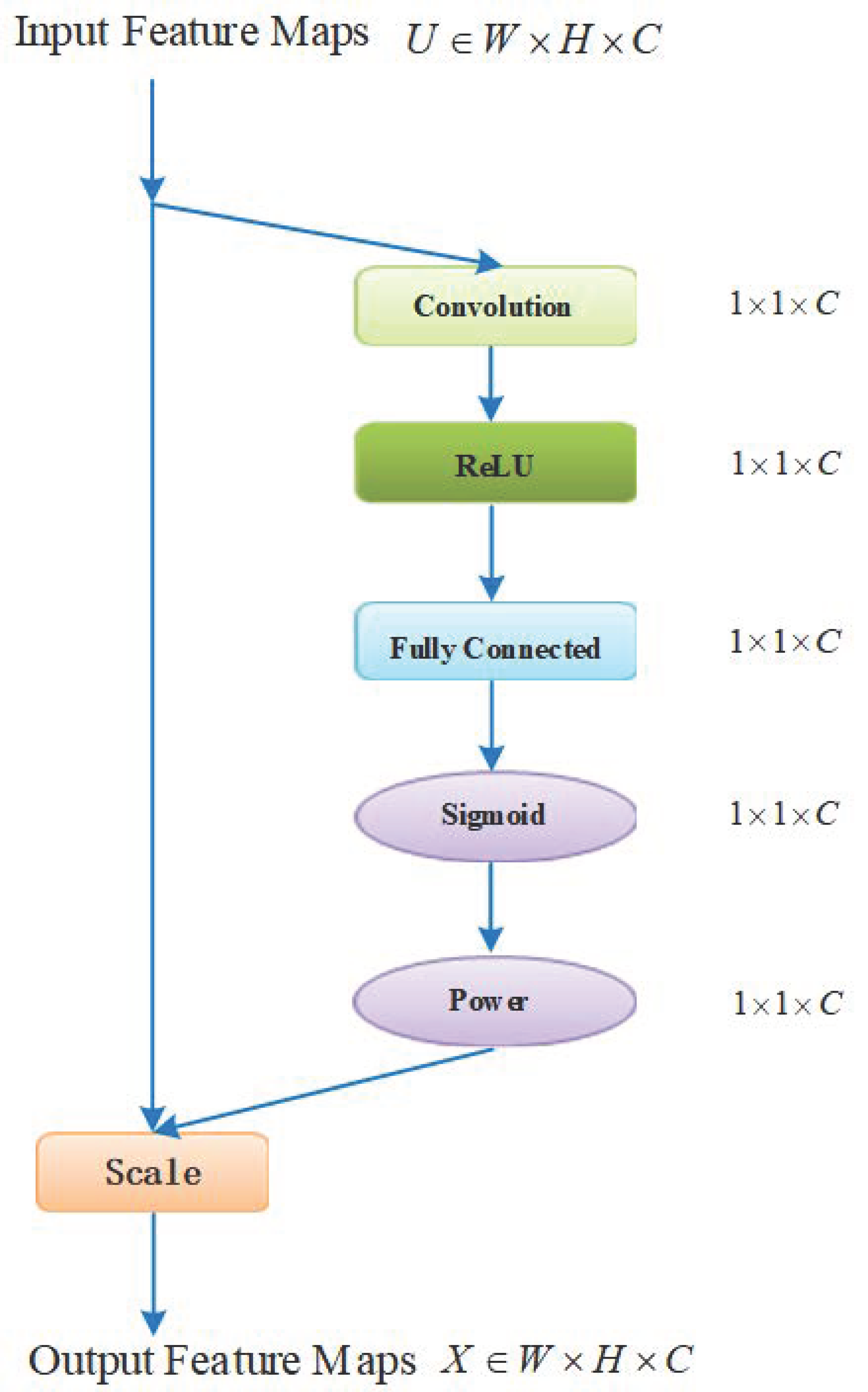
Figure 6 shows the structure of the enhanced-SE module with the above modification. Figure 7 shows an illustrative comparison between the feature maps output by the SE module and the enhanced-SE module in a SAR ATR task. Obviously, many feature maps become blank in Figure 7b, indicating that the enhanced-SE module suppresses feature maps with little information more effectively than the original SE module.

3.3. Other Components in the ESENet

The convolutional layer and pooling layer are the basic components in a typical CNN structure [34]. The convolutional layer often acts as a feature extractor, which convolutes the input with a convolutional kernel to generate the new feature map. The pooling layer is a subsampling layer that reduces the number of trainable parameters of the network. By subsampling, the structural feature of the current layer is maintained and the impact of the deformed training samples on feature extraction is reduced.

Neural networks are essentially utilized to fit the data distribution. If the training and test sets have different distributions, the convergence speed will decrease and the generalization performance will degrade. To tackle this problem, batch normalization is added behind the first convolutional layer of the ESENet to accelerate network training and improve the generalization performance.

Dropout is a common regularization method that is utilized in deep neural networks [35]. This technique randomly samples the weights from the current layer with probability p and prune them out, similar to the ensemble of sub-networks. Usually, it is adopted in the layer with a large number of parameters to alleviate overfitting. In the proposed ESENet, the fully-connected layer has a small number of parameters, while the third convolutional layer and the forth convolutional layer contain most of the trainable weights. Thus, we apply dropout in the two layers with p = 0.5 and p = 0.25, respectively.

Additionally, we replace the common softmax classifier by the LM-softmax classifier, which could improve the classification performance by adjusting the decision boundary of features that were extracted by CNN.

3.4. Parameter Settings and Training Method

We apply the gradient decent technique with weight decay and momentum in the training process [36], which is defined by:

$$\Delta {\theta }_{i+1}=\alpha ·\Delta {\theta }_i-\beta ·\epsilon ·{\theta }_i-\epsilon ·\frac{\partial L}{\partial \theta }$$

(6)

$${\theta }_{i+1}={\theta }_i+\Delta {\theta }_{i+1}$$

(7)

where $\Delta {\theta }_{i+1}$ is the variation of $\theta$ in the (i + 1)th iteration, $\epsilon$ is the learning rate, $\alpha$ is the momentum coefficient, $\beta$ is the weight decay coefficient, and $\frac{\partial L}{\partial \theta }$ is the derivative of loss function $L$ with respect to $\theta$. In this paper, the base learning rate is set to 0.02, $\alpha$ is set to 0.9, and $\beta$ is set to 0.004, respectively. Subsequently, we adopt a multi-step iteration strategy, which updates the learning rate to be $\epsilon =\epsilon /10$ if the iteration number reaches 1000, 2000, and 4000, etc. Additionally, we adopt a common training method that subtracts the mean of training samples from both the training and test samples to accelerate the convergence of CNN. In the enhanced-SE module, a is set to 0, b is set to 1, and q is set to 2. In the SE module, r is set to 16.

4. Experiments on MSTAR Dataset

4.1. Dataset Description

The training and test datasets are generated from the MSTAR dataset that was provided by DARPA/AFRL [13]. The dataset was collected by Sandia National Laboratory SAR sensor platform in 1995 and 1996 using an X-band SAR sensor. It provides a nominal spatial resolution of 0.3 × 0.3 m in both range and azimuth, and the image size is 128 × 128. The publicly released datasets include ten categories of ground military vehicles, i.e., armored personnel carrier: BMP-2, BRDM-2, BTR-60, and BTR-70; tank: T62, T72; rocket launcher: 2S1; air defense unit: ZSU-234; truck: ZIL-131; and, bulldozer: D7.

The MSTAR dataset consists of two sub-datasets for the sake of performance evaluation in various scenarios, i.e., the standard operating conditions (SOC) dataset and the extended operating conditions (EOC) dataset. The SOC dataset consists of ten target categories at 17° and 15° depression angles, respectively, as shown in

Table 1. Training and test samples for the standard operating conditions (SOC) experiments setup.

Class	Train		Test
	Depression	Number	Depression	Number
BMP-2	17°	698	15°	587
BTR-70	17°	233	15°	196
T-72	17°	691	15°	582
BTR-60	17°	256	15°	195
2S1	17°	299	15°	274
BRDM-2	17°	298	15°	274
D-7	17°	299	15°	274
T-62	17°	299	15°	273
ZIL-131	17°	299	15°	274
ZSU-234	17°	299	15°	274
Total	17°	3671	15°	3203

. As a matter of routine [12,21], images at 17° depression angle serve as training samples and images at the 15° depression angle serve as test samples.

The EOC dataset includes EOC1 and EOC2, i.e., large depression variation dataset and variants dataset. There are four target categories in EOC1, including 2S1, BRDM-2, T-72, and ZSU-234. Images at 17° depression angle serve as training samples and images at 30° depression angle serve as test samples, as shown in

Table 2. Number of training and test samples for extended operating conditions (EOC)-1 (large depression variation).

Class	Train		Test
	Depression	Number	Depression	Number
2S1	17°	299	30°	288
BRDM-2	17°	298	30°	287
T-72	17°	691	30°	288
ZSU-234	17°	299	30°	288

. There are two target categories in EOC2, i.e., configuration variants and version variants. For the configuration variants, the training samples include BMP2, BRDM-2, BTR-70, and T-72, and the test samples only include variants of T72. For version variants, the training samples include BMP-2, BRDM-2, BTR-70, and T-72, and the test samples include variants of T72 and BMP-2. Detailed information is listed in

Table 3. Number of training and test samples for EOC-2 (configuration variants).

Class	Train		Class	Test Variants
	Depression	Number		Depression	Number
BMP-2/9563	17°	233	T-72/S7	15° 17°	419
BRDM-2/E71	17°	298	T-72/A32	15° 17°	572
BTR-70/c71	17°	233	T-72/A62	15° 17°	573
T-72/132	17°	232	T-72/A63	15° 17°	573
			T-72/A64	15° 17°	573

and

Table 4. Number of training and test samples for EOC-2 (version variants).

Class	Train		Class	Test Variants
	Depression	Number		Depression	Number
BMP-2/9563	17°	233	T-72/812	15° 17°	426
BRDM-2/E71	17°	298	T-72/A04	15° 17°	573
BTR-70/c71	17°	233	T-72/A05	15° 17°	573
T-72/132	17°	232	T-72/A07	15° 17°	573
			T-72/A10	15° 17°	567
			BMP-2/9566	15° 17°	428
			BMP-2/C21	15° 17°	429

, respectively.

4.2. Network Structures for Comparison

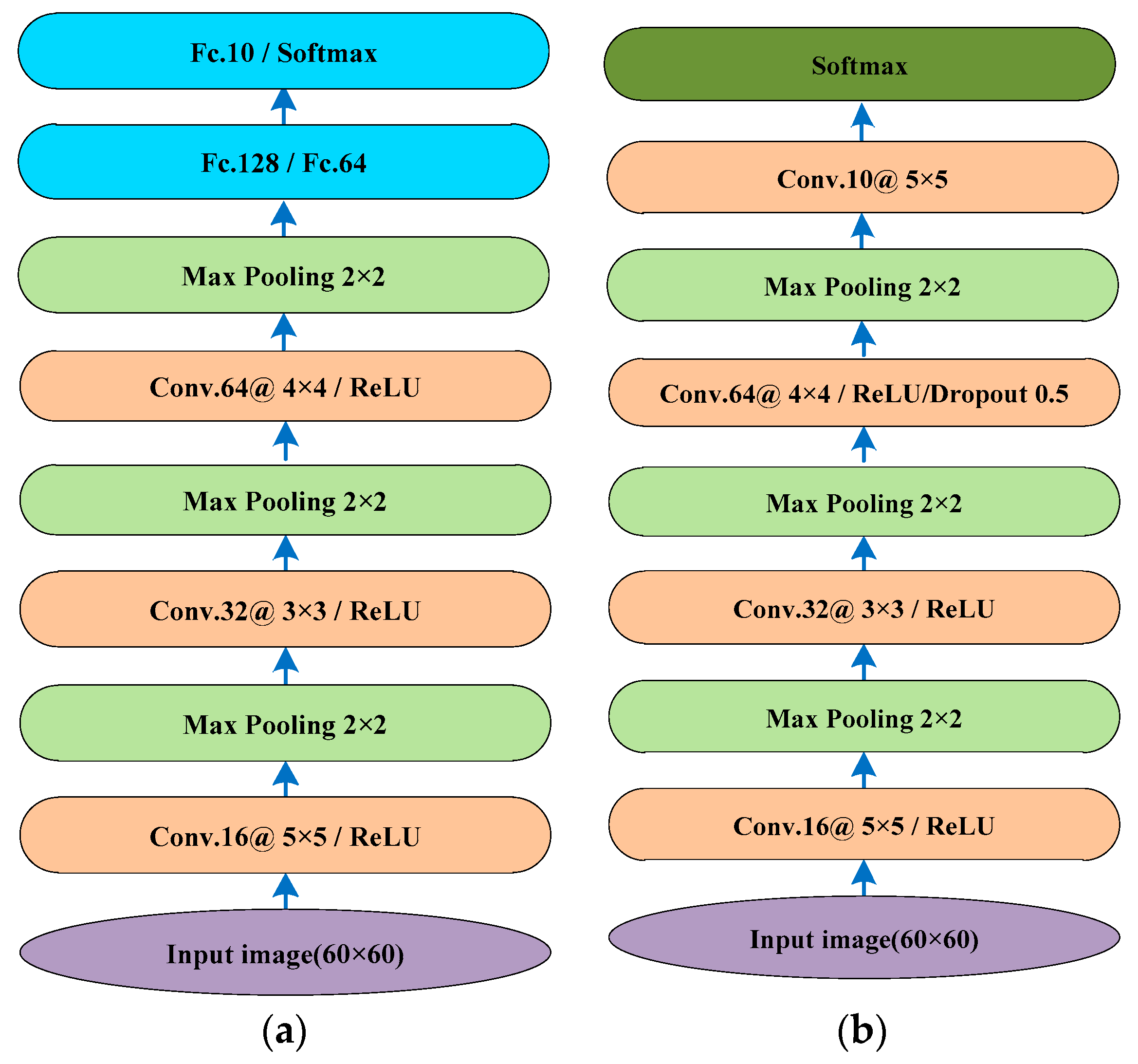
Traditional CNN and A-convnet structures are designed according to the size of the input image by referring to the structures given in references [12,21] for the convenience of comparison. Subsequently, structures yielding the highest classification accuracy are selected as optimal ones, as shown in Figure 8a,b, respectively. Data augmentation methods, such as translation and rotation, are not applied in this paper.

4.3. Effect of Clutter and Data Generation

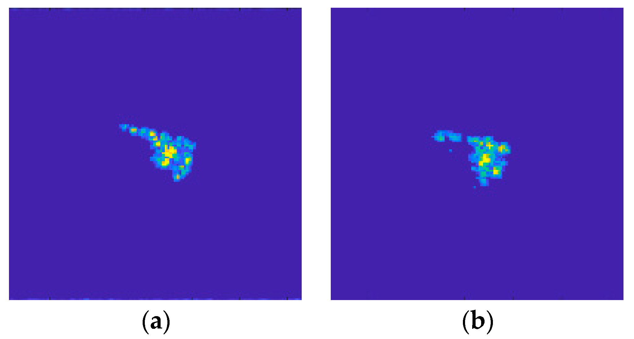
Reference [14] shows that, although the target region has been removed from original MSTAR images, the nearest neighbor classifier still achieves high classification accuracy, proving that the clutter in the training and test images of the MSTAR dataset is highly correlated. Reference [15] also proves that background clutter in the MSTAR dataset will disturb the recognition results of CNN. The target region is segmented out from the original SAR images according to references [15,30] to mitigate the impact of background clutter on network training and testing, as shown by Figure 9. The original 128 × 128 image is cropped to 60 × 60 to reduce the computational cost, because the target only occupies a small region at the center of the original image. By this means, the pure target dataset utilized in this paper is generated.

4.4. Results of SOC

Table 5. Recognition accuracy comparison under SOC.

	Traditional CNN	A-Convnet	SENet	ESENet
Accuracy (%)	94.79	95.04	96.63	97.32

shows the recognition results of ESENet and other CNN structures for comparison under SOC. We replace the enhanced-SE module in the ESENet with an original SE module and obtain the SENet for comparison in Table 5 to validate the effectiveness of the proposed enhanced-SE module.

Table 6. Confusion matrix of ESENet under SOC.

Class	BMP-2	BTR-70	T-72	BTR-60	2S1	BRDM-2	D7	T62	ZIL131	ZSU234	Acc (%)
BMP-2	584	0	3	0	0	0	0	0	0	0	99.49
BTR-70	0	195	0	0	0	1	0	0	0	0	99.49
T-72	5	0	575	0	0	0	0	1	0	1	98.80
BTR-60	0	0	0	189	1	5	0	0	0	0	96.92
2S1	3	0	1	0	265	3	0	2	0	0	96.72
BRDM-2	2	13	0	4	0	254	0	0	1	0	92.70
D7	0	0	0	0	2	0	271	0	0	1	98.91
T-62	0	0	16	1	0	0	0	249	7	0	91.21
ZIL-131	0	6	0	0	0	0	0	0	268	0	97.81
ZSU-234	0	0	3	0	0	0	3	1	0	267	97.45
Total											97.32

provides the confusion matrix of ESENet.

As shown in Table 5, the recognition accuracy for traditional CNN, A-convnet, SENet, and ESENet under SOC is 94.79%, 95.04%, 96.63% and 97.32%, respectively. Although the background clutter has been removed from SAR images, the ESENet still obtains good recognition performance, as the recognition rate of all types of targets exceeds 90%. Table 5 shows that SENet outperforms the traditional CNN structures for SAR ATR by inserting the SE module into a common CNN structure. Moreover, comparisons between the SENet and ESENet show that the enhanced-SE module outperforms the SE module in facilitating the feature extraction of CNN in a SAR ATR task.

For a typical test sample, the feature maps of ESENet before and after transformation by the SE and the enhanced-SE modules are shown in Figure 10. It is observed that the feature maps of the second convolutional layer that pass through the SE module almost unchanged. However, in the third convolutional layer, the feature maps with little information are effectively suppressed when they pass through the enhanced-SE module.

For the purpose of illustration, we present a sample of BTR-70 in Figure 11a, which is misclassified to BTR-60 by the SENet, while the ESENet correctly classifies it. The feature maps of the third convolutional layer in the SENet are shown in Figure 11c,d and the feature maps of the third convolutional layer in the ESENet are shown in Figure 11e,f. It is observed that the enhanced-SE module suppresses the feature maps with little information more effectively than the SE module.

4.5. Results of EOC1

Subsequently, the EOC1 dataset is utilized to evaluate the performance of ESENet under large depression angle variation. As shown in

Table 7. Recognition accuracy comparison under EOC1.

	Traditional CNN	A-Convnet	SENet	ESENet
Accuracy (%)	88.44	89.05	90.27	93.04

, the recognition accuracy of traditional CNN, the A-convnet, the SENet, and the ESENet is 88.44%, 89.05%, 90.27%, and 93.40% respectively, which shows that the ESENet outperforms the others under EOC1. However, the accuracy of the EOC1 experiment is lower than that of the SOC experiment. As expected, the large difference between the training and the test samples decreases the recognition accuracy, because the SAR image is sensitive to the variation of viewing angles.

Table 8. Confusion matrix of ESENet under EOC1.

Class	2S1	BRDM-2	T-72	ZSU-234	Acc (%)
2S1	282	2	3	1	97.92
BRDM-2	0	283	1	3	98.61
T-72	10	0	236	42	81.94
ZSU-234	3	0	11	274	95.14
Total					93.40

shows the confusion matrix of the ESENet under EOC1. It is observed that the recognition accuracy of T72 rapidly decreases, which might be caused by the similarity between T72 and ZSU-234 for large depression angle variation. As shown in Figure 12, the SAR image of T72 at 30° depression angle exhibits a configuration similarity to ZSU-234 at 17° depression angle.

4.6. Results of EOC2

Variants recognition plays a significant role in SAR ATR. We test the network’s ability to distinguish objects with similar appearance in the experiments under EOC2. For the configuration variants dataset that is introduced in Table 3,

Table 9. Recognition accuracy comparison under EOC2 (configuration variants).

Class	Subclass of Variants	Accuracy (%)
		Traditional CNN	A-Convent	SENet	ESENet
T-72	S7	83.05	79.95	82.34	84.25
	A32	86.89	89.16	93.88	93.01
	A62	92.84	94.42	95.81	95.46
	A63	90.05	89.35	89.70	91.45
	A64	79.76	81.68	83.77	85.86
Total		86.72	87.31	89.48	90.33

shows the recognition accuracy of the above-mentioned four networks and

Table 10. Confusion matrix of ESENet under EOC2 (configuration variants).

Class	Variants	BMP-2	BTR-70	T-72	BRDM-2	Acc (%)
T-72	S7	59	6	353	1	84.25
	A32	38	0	532	2	93.01
	A62	24	2	547	0	95.46
	A63	49	0	524	0	91.45
	A64	72	8	492	1	85.86
Total						90.33

shows the confusion matrix of the ESENet. Obviously, the ESENet outperforms the others and the recognition accuracy is increased by 3% as compared with traditional CNN. For the version variants dataset that is introduced in Table 4,

Table 11. Recognition accuracy comparison under EOC2 (version variants).

Class	Subclass of Variants	Accuracy (%)
		Traditional CNN	A-Convent	SENet	ESENet
BMP-2	9566	92.52	92.52	92.29	92.99
	c21	93.01	93.47	95.57	95.80
T-72	812	88.03	90.14	89.44	92.96
	A04	77.84	78.71	82.55	84.82
	A05	89.70	91.10	90.75	92.32
	A07	79.76	82.02	81.15	83.25
	A10	85.01	85.36	86.07	86.77
Total		85.99	87.08	87.76	89.35

lists the recognition accuracy of the four networks, and

Table 12. Confusion matrix of ESENet under EOC2 (configuration variants).

Class	Variants	BMP-2	BTR-70	T-72	BRDM-2	Acc (%)
BMP-2	9566	398	5	10	15	92.99
	c21	411	2	10	6	95.80
T-72	812	26	4	396	0	92.96
	A04	81	3	486	3	84.82
	A05	43	1	529	0	92.32
	A07	95	1	477	0	83.25
	A10	74	1	492	0	86.77
Total						89.35

lists the confusion matrix of the ESENet. It is observed that the ESENet has the best recognition performance among the four CNN structures.

5. Conclusions

Feature extraction plays an important role in the task of SAR ATR. This paper proposed the ESENet to solve the problem that feature maps with little information being automatically learned by CNN will decrease the SAR ATR performance. In this framework, we designed a new enhanced-SE module. The enhanced-SE module could enhance the ability of CNN in suppressing feature maps with little information by computing and allocating different weights to the corresponding feature maps. For the preprocessed MSTAR dataset, experiments have shown that the ESENet achieves higher recognition accuracy than traditional CNN structure and A-convent, and that it exhibits robustness to large depression angle variation, configuration variants, and version variants.

Future work will be focused on network optimization, multi-channel CNN structure designing for multi-dimensional feature extraction, and improving the network robustness to the distorted datasets.

References

- Dudgeon, D.; Lacoss, R. An overview of automatic target recognition. Lincoln Lab. J. 1993, 6, 3–10. [Google Scholar]
- Park, J.; Kim, K. Modified polar mapping classifier for SAR automatic target recognition. IEEE Trans. Aerosp. Electron. Syst. 2014, 50, 1092–1107. [Google Scholar] [CrossRef]
- Novak, L.; Owirka, G.; Brower, W.; Weaver, A. The automatic target-recognition system in SAIP. Lincoln Lab. J. 1997, 10, 187–201. [Google Scholar]
- Owirka, G.; Verbout, S.; Novak, L. Template-based SAR ATR performance using different image enhancement techniques. Proc. SPIE 1999, 3721, 302–319. [Google Scholar]
- Novak, L. State-of-the-art of SAR automatic target recognition. In Proceedings of the 2000 IEEE International Radar Conference, Alexandria, VA, USA, 12 May 2000; pp. 836–843. [Google Scholar]
- DeVore, M.; O’Sullivan, J. A performance complexity study of several approaches to automatic target recognition from synthetic aperture radar images. IEEE Trans. Aerosp. Electron. Syst. 2000, 38, 632–648. [Google Scholar]
- Chiang, H.; Moses, R.; Potter, L. Model-based classification of radar images. IEEE Trans. Inf. Theory 2000, 46, 1842–1854. [Google Scholar] [CrossRef]
- Darymli, K.; Mcguire, P.; Gill, E.; Power, D. Holism-based features for target classification in focused and complex-valued synthetic aperture radar imagery. IEEE Trans. Aerosp. Electron. Syst. 2016, 52, 786–808. [Google Scholar] [CrossRef]
- Huang, X.; Qiao, H.; Zhang, B. SAR target configuration recognition using tensor global and local discriminant embedding. IEEE Geosci. Remote Sens. Lett. 2016, 13, 222–226. [Google Scholar] [CrossRef]
- Deng, S.; Du, L.; Li, C.; Ding, J.; Liu, H. SAR automatic target recognition based on Euclidean distance restricted autoencoder. IEEE J. Sel. Top. Appl. Earth Obs. 2017, 10, 1–11. [Google Scholar] [CrossRef]
- Mahdianpari, M.; Salehi, B.; Rezaee, M.; Mohammadimanesh, F.; Zhang, Y. Very deep convolutional neural networks for complex land cover mapping using multispectral remote sensing imagery. Remote Sens. 2018, 10, 1119. [Google Scholar] [CrossRef]
- Chen, S.; Wang, H.; Xu, F.; Jin, Y. Target classification using the deep convolutional networks for SAR images. IEEE Trans. Geosci. Remote Sens. 2016, 8, 4806–4817. [Google Scholar] [CrossRef]
- Defense Advanced Research Projects Agency (DARPA); Air Force Research Laboratory (AFRL). The Air Force Moving and Stationary Target Recognition Database. Available online: https://www.sdms.afrl.af.mil/index.php?collection=mstar (accessed on 5 April 2019).
- Schumacher, R.; Schiller, J. Non-cooperative target identification of battlefield targets classification results based on SAR images. In Proceedings of the IEEE International Radar Conference, Arlington, VA, USA, 9–12 May 2005; pp. 167–172. [Google Scholar]
- Zhou, F.; Wang, L.; Bai, X.; Hui, Y. SAR ATR of Ground Vehicles Based on LM-BN-CNN. IEEE Trans. Geosci. Remote Sens. 2018, 56, 7282–7293. [Google Scholar] [CrossRef]
- Ding, J.; Chen, B.; Liu, H.; Huang, M. Convolutional neural network with data augmentation for SAR target recognition. IEEE Geosci. Remote Sens. Lett. 2016, 13, 364–368. [Google Scholar] [CrossRef]
- Wagner, S. SAR ATR by a combination of convolutional neural network and support vector machines. IEEE Trans. Aerosp. Electron. Syst. 2017, 52, 2861–2872. [Google Scholar] [CrossRef]
- Lin, Z.; Ji, K.; Kang, M.; Leng, X.; Zou, H. Deep convolutional highway unit network for SAR target classification with limited labeled training data. IEEE Geosci. Remote Sens. Lett. 2017, 14, 1091–1095. [Google Scholar] [CrossRef]
- Shang, R.; Wang, J.; Jiao, L.; Stolkin, R.; Hou, B.; Li, Y. SAR targets classification based on deep memory convolution neural networks and transfer parameters. IEEE J. Sel. Top. Appl. Earth Obs. 2018, 11, 2834–2846. [Google Scholar] [CrossRef]
- Wang, J.; Zheng, T.; Lei, P.; Bai, X. Ground target classification in noisy SAR images using convolutional neural networks. IEEE J. Sel. Top. Appl. Earth Obs. 2018, 11, 4180–4192. [Google Scholar] [CrossRef]
- Morgan, D. Deep convolutional neural networks for ATR from SAR imagery. Proc. SPIE 2015, 9475, 94750F. [Google Scholar]
- Hansen, D.; Kusk, A.; Dall, J.; Nielsen, A.; Engholm, R.; Skriver, H. Improving SAR automatic target recognition models with transfer learning from simulated data. IEEE Geosci. Remote Sens. Lett. 2017, 99, 1–5. [Google Scholar]
- Huang, Z.; Pan, Z.; Lei, B. Transfer learning with deep convolutional neural network for SAR target classification with limited labeled data. Remote Sens. 2017, 9, 907. [Google Scholar] [CrossRef]
- Wagner, S. Combination of convolutional feature extraction and support vector machines for radar ATR. In Proceedings of the 17th International Conference on Information Fusion, Salamanca, Spain, 7–10 July 2014. [Google Scholar]
- Kechagias-Stamatis, O.; Aouf, N. Fusing deep learning and sparse coding for SAR ATR. IEEE Trans. Aerosp. Electron. Syst. 2019, 55, 785–797. [Google Scholar] [CrossRef]
- Pei, J.; Huang, Y.; Huo, W.; Zhang, Y.; Yang, J.; Yeo, T.S. SAR Automatic Target Recognition Based on Multiview Deep Learning Framework. IEEE Trans. Geosci. Remote Sens. 2018, 56, 2196–2210. [Google Scholar] [CrossRef]
- Li, H.; Kadav, A.; Durdanovic, I.; Samet, H.; Graf, H. Pruning filters for efficient convnets. In Proceedings of the 2017 International Conference on Learning Representation (ICLR), Toulon, France, 24–26 April 2017; pp. 1–13. [Google Scholar]
- He, Y.; Zhang, X.; Sun, J. Channel pruning for accelerating very deep neural networks. In Proceedings of the 2017 International Conference on Computer Vision (ICCV), Venice, Italy, 22–29 October 2017. [Google Scholar]
- Hu, S.; Shen, L.; Sun, G. Squeeze-and-Excitation Networks. arXiv 2017, arXiv:1709.01507. [Google Scholar]
- Meth, R. Target/shadow segmentation and aspect estimation in synthetic aperture radar imagery. Proc. SPIE 1998, 3370, 188–196. [Google Scholar]
- Liu, L.; Wen, Y.; Yu, Z.; Yang, M. Large-margin softmax loss for convolutional neural networks. In Proceedings of the 33rd International Conference on Machine Learning (ICML), New York, NY, USA, 19–24 June 2016; pp. 507–516. [Google Scholar]
- Ioffe, S.; Szegedy, C. Batch Normalization: Accelerating deep network training by reducing internal covariate shift. In Proceedings of the 32nd International Conference on International Conference on Machine Learning (ICML), Lille, France, 6–12 July 2015; pp. 448–456. [Google Scholar]
- Bishop, C. Pattern Recognition and Machine Learning; Springer: New York, NY, USA, 2008; p. 197. ISBN 978-0-387-31073-2. [Google Scholar]
- LeCun, Y.; Bottou, L.; Bengio, Y.; Haffner, P. Gradient-based learning applied to document recognition. Proc. IEEE 1998, 86, 2278–2324. [Google Scholar] [CrossRef] [Green Version]
- Srivastava, N.; Hinton, G.; Krizhevsky, A.; Sutskever, I.; Salakhutdinov, R. Dropout: A simple way to prevent neural networks from overfitting. J. Mach. Learn. Res. 2014, 15, 1929–1958. [Google Scholar]
- LeCun, Y.; Bottou, L.; Orr, G.; Muller, K. Efficient backprop. In Neural Networks: Tricks of the Trade; Springer: Berlin, Germany, 2012; pp. 9–48. [Google Scholar]
Figure 1.
Illustration of feature maps learned by convolutional neural network (CNN) in a synthetic aperture radar automatic target recognition (SAR ATR) experiment.
Figure 2.
The structure of the Squeeze and Excitation (SE) module.
Figure 3.
Overview of the proposed SAR ATR method.
Figure 4.
Structure of the Enhanced Squeeze and Excitation Net (ESENet).
Figure 5.
Comparison between the sigmoid function and the enhanced-sigmoid function.
Figure 6.
Structure of the enhanced-SE module.
Figure 7.
Visualization of feature maps output by the SE module (a) and the enhanced-SE module (b).
Figure 8.
Optimal structures of traditional CNN (a) and A-convnet (b) for the 60 × 60 input image.
Figure 9.
Illustration of target region segmentation: (a) original SAR image; (b) segmented image.
Figure 10.
Visualization of feature maps in the ESENet. (a) input image; (b) mean of training samples; (c) input image with the mean of the training samples removed; (d) feature maps of conv2; (e) feature maps of conv2 after passing through the SE module; (f) feature maps of conv3; and, (g) feature maps of conv3 after passing through the enhanced-SE module.
Figure 11.
Feature maps of conv3 in SENet and ESENet. (a) input image; (b) input image with the mean of training samples removed; (c) feature maps of conv3 in the SENet; (d) feature maps of conv3 in the SENet after passing through the SE module; (e) feature maps of conv3 in the ESENet; and, (f) feature maps of conv3 in the ESENet after passing through the enhanced-SE module.
Figure 12.
SAR image comparison with large depression angle variation. (a) image of T72 at 30° depression angle; and, (b) image of ZSU-234 at 17° depression angle.