A Computationally Efficient Semantic SLAM Solution for Dynamic Scenes

Abstract

In various dynamic scenes, there are moveable objects such as pedestrians, which may challenge simultaneous localization and mapping (SLAM) algorithms. Consequently, the localization accuracy may be degraded, and a moving object may negatively impact the constructed maps. Maps that contain semantic information of dynamic objects impart humans or robots with the ability to semantically understand the environment, and they are critical for various intelligent systems and location-based services. In this study, we developed a computationally efficient SLAM solution that is able to accomplish three tasks in real time: (1) complete localization without accuracy loss due to the existence of dynamic objects and generate a static map that does not contain moving objects, (2) extract semantic information of dynamic objects through a computionally efficient approach, and (3) eventually generate semantic maps, which overlay semantic objects on static maps. The proposed semantic SLAM solution was evaluated through four different experiments on two data sets, respectively verifying the tracking accuracy, computational efficiency, and the quality of the generated static maps and semantic maps. The results show that the proposed SLAM solution is computationally efficient by reducing the time consumption for building maps by 2/3; moreover, the relative localization accuracy is improved, with a translational error of only 0.028 m, and is not degraded by dynamic objects. Finally, the proposed solution generates static maps of a dynamic scene without moving objects and semantic maps with high-precision semantic information of specific objects.

1. Introduction

A dynamic scene contains various moveable objects, such as pedestrians. It is important for intelligent systems and location-based services [1] to recognize in real time such dynamic objects and construct scene maps with semantic information of dynamic objects. For example, a robot needs to understand what objects are in the scene and where such objects are located so that the robot can perform more intelligently. This task can be accomplished by combining a semantic segmentation network and mobile mapping. However, dynamic objects in the scene will challenge the localization and mobile mapping, which is largely accomplished by simultaneous localization and mapping (SLAM) [2] algorithms. Dynamic objects in a scene will degrade the localization accuracy of SLAM processing, and moving objects will degrade the quality of the generated maps. Since the real world contains dynamic objects, current approaches are prone to failure, the pose estimation might drift or even be lost as there are false correspondences or not sufficiently many features to be matched [3]. A pedestrian may appear in several continuous images, and the resulting generated map is negatively impacted with a blurry pedestrian. In addition, if the dynamic object in the scene is a non-rigid object, the result will be worse because we need to handle deformable objects in a SLAM context [4,5]. Meanwhile, a mobile platform such as a robot has limited computational capability, and it is difficult to synchronously implement a semantic segmentation network and mobile mapping in real time [6,7]. A computationally efficient solution for synchronously extracting object semantic information and mobile mapping will enable a variety of novel intelligent systems and applications.

Vision-based SLAM has been developed for a long time and mainly solves two problems: the first is estimating the camera trajectory, and the second is reconstructing the geometry of the environment at the same time. In recent years, keyframe-based SLAM has almost become the dominant technique. According to Strasdat et al. [8], keyframe-based techniques are more accurate than filtering-based approaches. Keyframe-based parallel tracking and mapping (PTAM) [9] was once regarded by many scholars as the gold standard in monocular SLAM [10]. Currently, the most representative keyframe-based systems are probably ORB-SLAM2 [10] and DSO [11], both of which achieve unprecedented performance with respect to other state-of-the-art visual SLAM approaches in terms of localization accuracy. However, their shortcomings are also clear. These approaches are not good at building maps, and the generated sparse point cloud map is not sufficient for the intelligent autonomous navigation of robots.

Semantic SLAM incorporates artificial intelligence methods, such as deep learning, with SLAM processing, and it can achieve the calculation of scene geometry mapping and semantic object extraction simultaneously, which is of great importance for autonomous robots and intelligent systems. Nüchter [12] first proposed the concept of constructing semantic maps for mobile robots in 2008. In 2011, Bao [13] proposed the reconstruction of semantic scenes using semantic information and SFM. Salas-Moreno [14] proposed an “object-oriented” SLAM system (SLAM++) in 2013. SLAM++ first constructed the point cloud map of a scene with an RGB-D camera, and then it recognized 3D objects in the scene using the point cloud map. Finally, fine 3D models prepared beforehand are added to the point cloud map. Considering that there are many features of non-object structures in the scene, Salas-Moreno [15] proposed a dense plane SLAM algorithm in 2014 to improve semantic SLAM by detecting the plane in the scene. Vineet [16] proposed a real-time, binocular, large-scene semantic reconstruction algorithm in 2015. This algorithm first segmented the image through a random forest, then reconstructed the three-dimensional scene with KinectFusion, and finally corrected it with a conditional random field. Leutenegger and McCormac [17] proposed SemanticFusion in 2016, which combines ElasticFusion with a convolutional neural network (CNN). SemanticFusion is semantically segmented by the CNN and then constructs semantic maps with ElasticFusion.

Although the established semantic SLAM methods have achieved good performance, there are still several aspects to be improved. (1) The computational efficiency of mapping needs to be enhanced such that it can be applied on a mobile platform, such as a robot, in real time. The current methods build a map with much more information than needed, which will largely reduce the efficiency of SLAM. (2) The adaptability to the dynamic environment needs to be enhanced. In a dynamic environment, moving objects appear in the map when using the current methods, which will bring difficulties to map applications, such as using maps for path planning. (3) The semantic segmentation accuracy of objects needs to be improved. The semantic segmentation result of the current method is not accurate enough for the robot to understand the scene correctly.

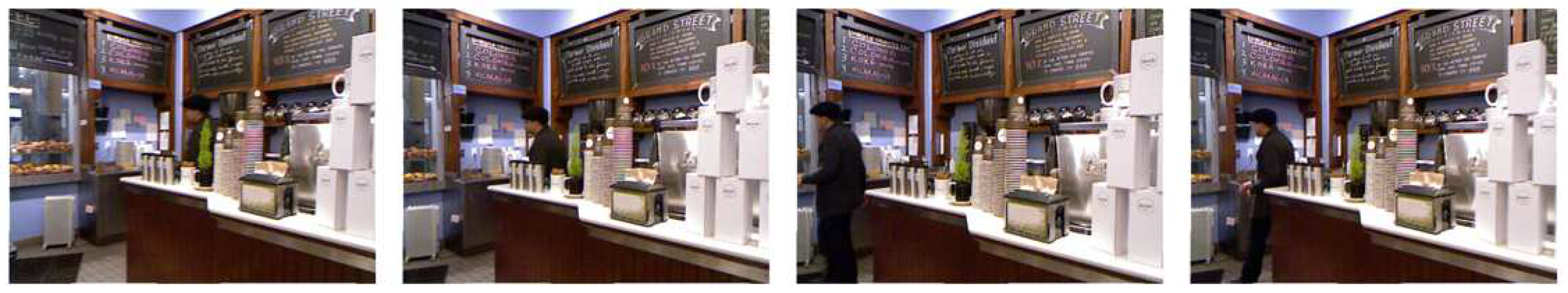
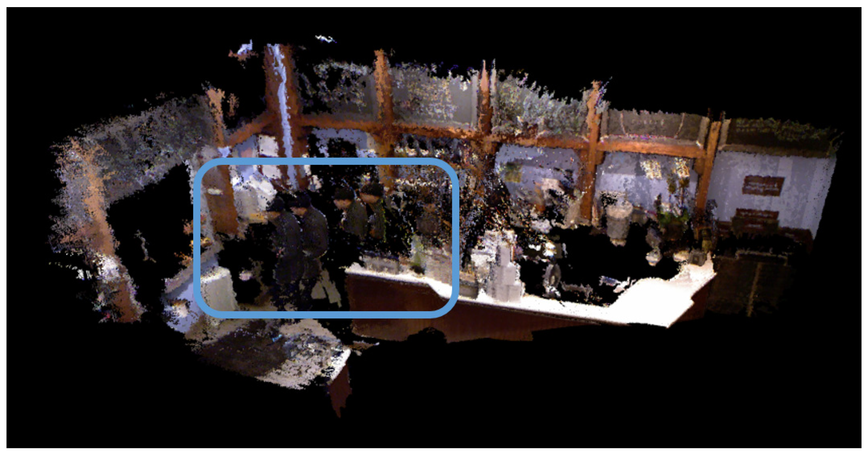
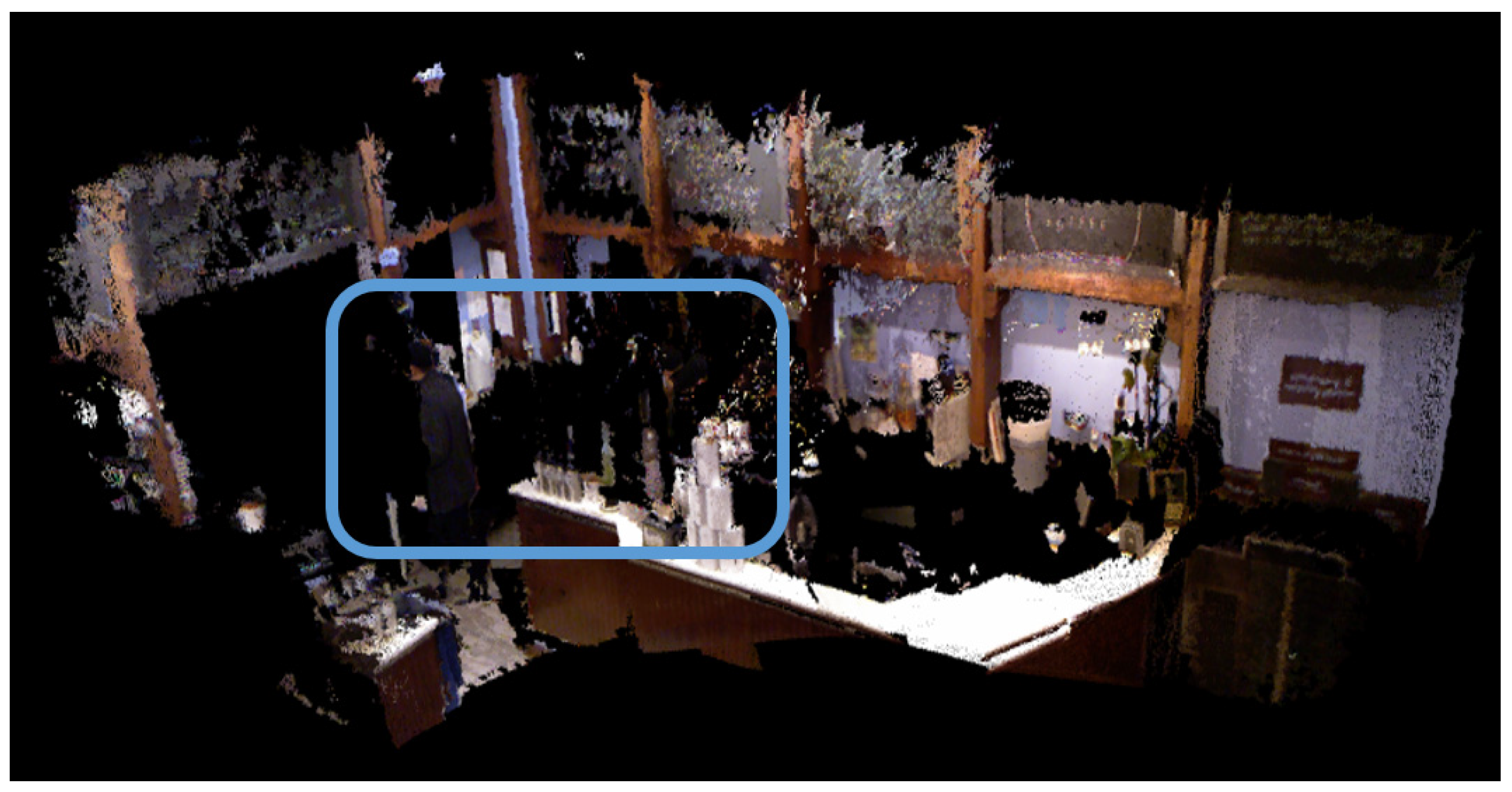
Figure 1 shows several keyframe images selected by the traditional visual SLAM system (ORB-SLAM2). Comparing several images shows that the similarity between adjacent keyframes is 90% or even 95%, which will bring substantial redundant information to the SLAM algorithm when constructing a dense point cloud map, and the redundant information will significantly increase the computational complexity but without any benefit for the quality of mapping. When there are moving targets in the scene, the residual image of the moving object will appear in the dense point cloud map constructed by keyframe-based SLAM, as shown in Figure 2.

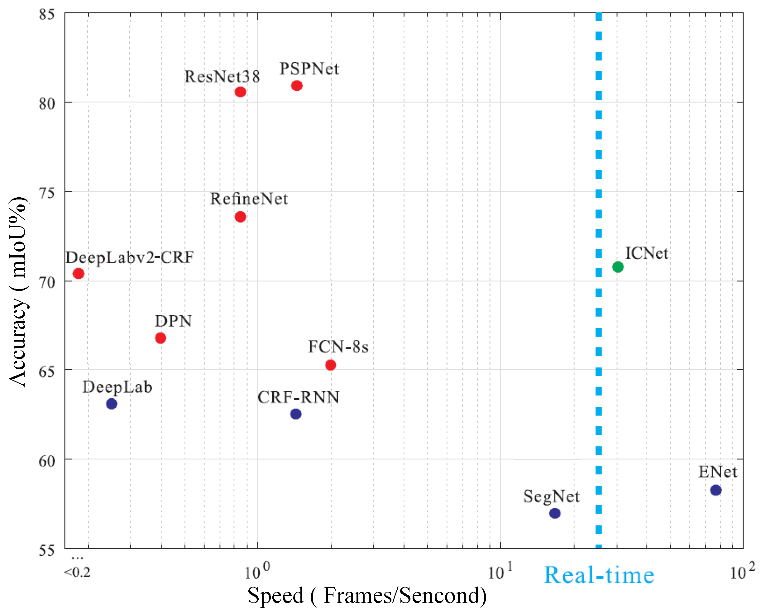
Traditional visual SLAM methods construct only a geometric map of a scene and are not able to address semantic information of the scene. Semantic SLAM methods combine visual SLAM with semantic segmentation networks, and they have high computational complexity, which is challenging for real-time systems. Figure 3 shows the inference speed and accuracy of the current semantic segmentation network, and we find that it is difficult to balance the accuracy and speed of segmentation. The semantic segmentation network with the highest accuracy in Figure 3 is PSPNet [18]. Its segmentation accuracy is approximately 81%, while its segmentation speed is only approximately 1.5 frames per second. The fastest semantic segmentation network is ENet [19], with a segmentation speed of approximately 75 frames per second and a segmentation accuracy of only approximately 58%. The compromise is ICNet [20], which can also achieve real-time performance, but its segmentation accuracy is not satisfactory.

In this paper, a semantic SLAM solution is proposed, and it achieves high-precision single-object semantic segmentation and generates semantic maps of a dynamic scene in real time. Our contributions are as follows:

• A lookup table (LUT) method is proposed for the first time to our knowledge. This method is applied in SLAM to improve the relative positioning accuracy of SLAM by increasing the number of feature points and distributing the feature points evenly, and it improves the efficiency of map reconstruction because it reduces redundant information that is not useful for building maps in the data.
• This study addresses the impact of dynamic objects on SLAM, and it detects and removes moving objects from the scene and generates the static map of a dynamic scene without moving objects.
• In contrast to traditional object semantic segmentation methods, the proposed solution adopts a step-wise approach that consists of object detection and contour extraction. The step-wise approach significantly reduces the computational complexity and makes the semantic segmentation process capable of operating in real time.
• The proposed solution incorporates the semantic information of objects with the SLAM process, and it eventually generates semantic maps of a dynamic scene, which is significant for semantic-information-based intelligent applications.

The remainder of this paper is organized as follows. A brief introduction to the framework is presented in Section 2. Details of the key techniques are described in Section 3 and Section 4. The experimental results are shown in Section 5. Finally, Section 6 provides the conclusion.

2. Overview of the Framework

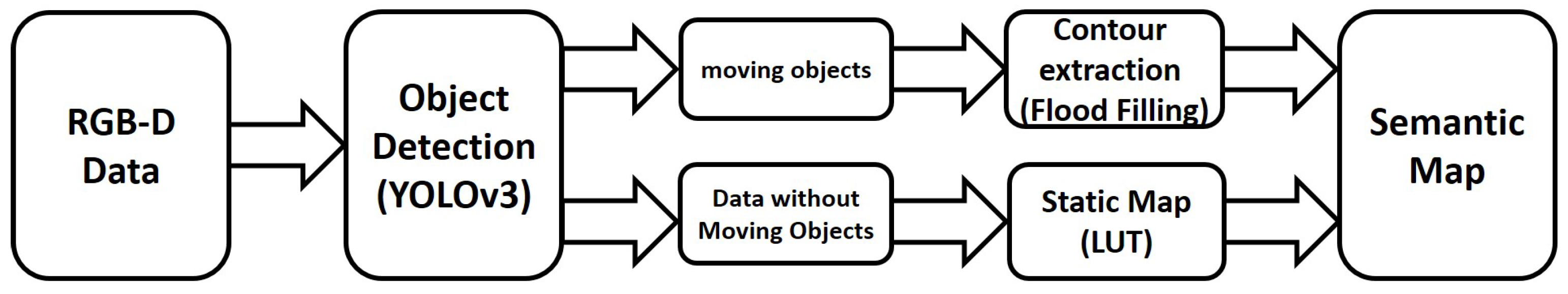
As shown in Figure 4, a general overview of the proposed solution mainly consists of four modules: object detection module, static map generation module, object contour extraction module and semantic map generation module. In this study, a static map refers to the dense point cloud map of a scene space excluding moveable objects, and a semantic map refers to the combination of a static map and corresponding semantic objects in the scene. The system uses an RGB-D camera sensor such as Kinect or RealSense. By processing the RGB-D input data with an offline training deep learning network, it can detect specific objects in the scene, such as pedestrians in a dynamic scene or cups on a table, and remove the moving objects in the SLAM process. In other words, the data without moving objects will be processed in localization and mapping. The static map module is based on the object detection module, and it uses the lookup table to improve the accuracy of SLAM and the efficiency of building maps. It can generate static maps of the dynamic scenes. The contour extraction module uses the depth map-based flood filling algorithm for extracting the contour of the result of the object detection, and it can obtain the high-precision semantic segmentation result of the specific object. Finally, the semantic map module combines the static map with the semantic information of the specific object, and it generates a semantic map with the semantic tag of the specific object.

3. Semantic Segmentation of Objects

In this study, we applied the state-of-the-art object detection network YOLOv3 for the detection of specific moving objects, and then we used the depth map-based flood filling algorithm for extracting the contour of specific objects. It can acquire highly precise semantic segmentation results of specific objects with a reduced computational complexity.

3.1. Object Detection with Deep Learning

Deep learning networks for object detection have developed very rapidly in recent years. The most highlighted methods include R-CNN [29], Fast R-CNN [30], Faster R-CNN [31], MasK R-CNN [32], SSD [33] and YOLO [34,35,36]. YOLOv3 [36] is currently the preferred method due to its comprehensive excellent performance, and its network structure is shown in

Table 1. YOLOv3 network structure.

Type	Filters	Size	Output
Convolutional	32	3 × 3	256 × 256
Convolutional	64	3 × 3 / 2	128 × 128
Convolutional	32	1 × 1		×1
Convolutional	64	3 × 3
Residual			128 × 128
Convolutional	128	3 × 3 / 2	64 × 64
Convolutional	64	1 × 1		×2
Convolutional	128	3 × 3
Residual			64 × 64
Convolutional	256	3 × 3 / 2	32 × 32
Convolutional	128	1 × 1		×8
Convolutional	256	3 × 3
Residual			32 × 32
Convolutional	512	3 × 3 / 2	16 × 16
Convolutional	256	1 × 1		×8
Convolutional	512	3 × 3
Residual			16 × 16
Convolutional	1024	3 × 3 / 2	8 ×8
Convolutional	512	1 × 1		×8
Convolutional	1024	3 × 3
Residual			8 × 8
Avgpool		Global
Connected		1000
Softmax

. The speed and accuracy can be adjusted by changing the size of the model structure.

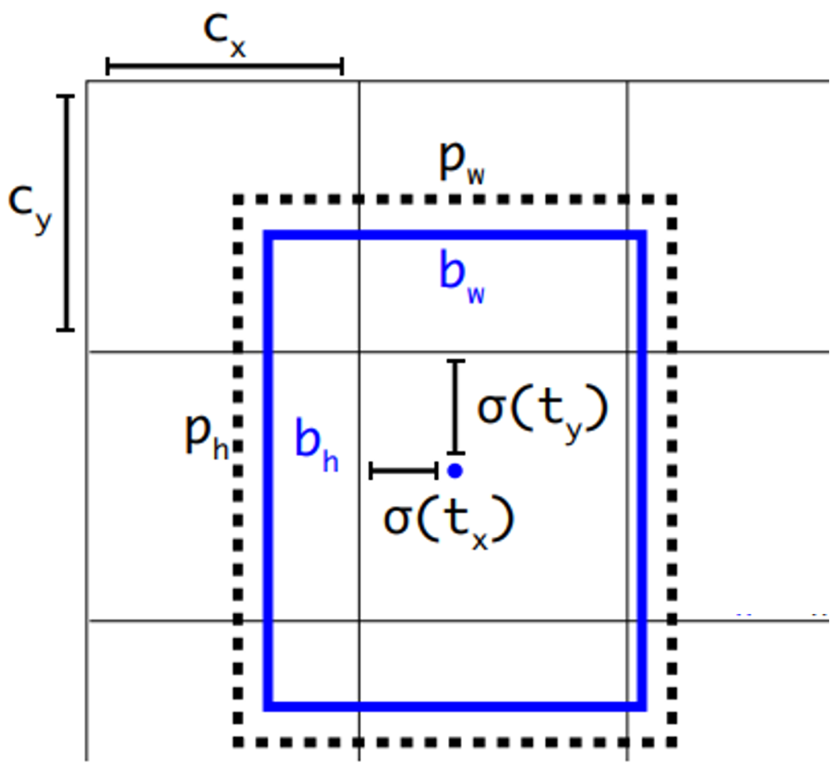
As shown in Figure 5, YOLOv3 predicts bounding boxes using dimension clusters as anchor boxes. The network predicts 4 coordinates $(t_x,t_y,t_w,t_h)$ for each bounding box by using the sum of squared error loss, where $t_x,t_y,t_w$ and $t_h$ represent the horizontal and vertical coordinates of the bounding box centre point and the length and width of the bounding box, respectively.

If the cell is offset from the top left corner of the image by $(c_x,c_y)$ and the bounding box prior has width and height $(p_w,p_h)$, then the predictions correspond to:

$$\begin{array}{c}{b}_x=\sigma \left(t_x\right)+c_x\hfill \\ b_y=\sigma \left(t_y\right)+c_y\hfill \\ b_w=p_w{e}^{t_w}\hfill \\ b_h=p_h{e}^{t_h}\hfill \end{array}$$

YOLOv3 predicts an object score for each bounding box using logistic regression. This score should be 1 if the bounding box prior overlaps a ground-truth object by more than any other bounding box prior. If the overlap is not more than some threshold (YOLOv3 is set to 0.5), then the prediction is ignored. In addition, YOLOv3 uses independent logistic classifiers for the class predictions. The loss function is binary cross-entropy loss.

3.2. Contour Extraction of Moving Objects

This study applied the depth map-based flood filling algorithm for extracting the contour of a moving object. The depth map-based flood filling algorithm determines whether the pixel belongs to the connected region of the seed point by evaluating whether the depth value of the pixel is the close to the depth value of the seed point, and it then fills the connected region with the specified colour to achieve the block segmentation effect of the image. Namely the flood filling algorithm uses the specified colour to fill the connected region. The key of the flood filling algorithm is actually to determine the connected region of the image. The implementation of the flood filling algorithm mainly includes two methods: seed filling method and scan line filling method.

The seed filling method is to recursively scan the four-neighbourhood or eight-neighbourhood pixels of the seed point until all pixels have been traversed or the contour boundary line of the target is found, i.e., the connected region is closed. The seed filling method is simple and intuitive, and it is easy to program. However, since the correlation between adjacent pixels is not considered, each pixel may be traversed multiple times; thus, its running efficiency is low, particularly when the connected area is larger, and the time consumption will substantially increase.

The scan line filling method does not detect the connected region by sequentially scanning the four-neighbourhood or the eight-neighbourhood pixels of the seed point but rather by detecting the area connected to the seed point in the current line to the left and right two directions from the seed point and then evaluating the pixels connected to the connected region in the upper and lower two lines of the current row. In this way, the upper and lower two rows of pixels of the connected region are scanned in turn until all the pixels are traversed or the contour boundary of the target is found. The scan line filling method considers the correlation between the four-neighbourhood or the eight-neighbourhood pixels of the seed point, and it avoids the repeated detection of the pixel points by progressive scanning, thereby greatly improving the efficiency of the operation.

In this paper, the eight-neighbourhood seed filling method is used to segment the target area of the object detection network output, and the semantic information for the segmentation target is provided by the target detection network. The specific algorithm steps are shown in Algorithm 1.

Algorithm 1 Depth Map-Based Flood Filling Algorithm.

1: Select the target area centre of the object detection network output as the initial seed point. 2: A new seed point is determined by evaluating whether the depth value difference between the pixel depth value of the eight-neighbourhood of the seed point and the pixel depth value of the seed point is within a certain threshold, i.e., the pixel depth value of the new seed point is in a certain threshold value, and is expressed as a formula. $$|DEPTH-depth|\le threshold$$ (1) where DEPTH is depth value of eight-neighbourhood pixels, and depth is depth value of the seed point. 3: When the new seed point is detected, the colour is replaced by the specified RGB. 4: The circumscribed rectangle is represented by the coordinates of the upper left corner and the coordinates of the lower right corner, and then all the non-seed points in the circumscribed rectangular area are traversed by repeating steps 2 and 3, and the update of the connected region is finally completed. The termination condition is that until all the pixels are traversed or the contour boundary line of the target is found, i.e., the closed connection area.

4. Generating Static Maps Using LUT-Based SLAM

The process of building a static map consists of removing the dynamic target by using the target detection module and then using the LUT method to improve the performance of SLAM. The LUT method can make feature points evenly distributed, improve SLAM positioning accuracy, reduce image redundancy information, and improve the efficiency of SLAM mapping.

4.1. Tracking

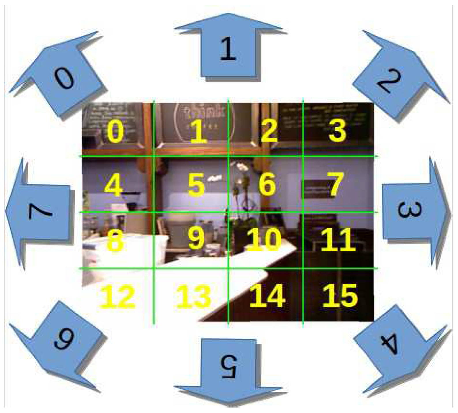
The image is equally divided into 16 cells in the first stage, as shown in Figure 6. The number 16 is used just as an example in this paper; however, an image should be divided into at least four tiles. Then, we extract a certain number of SIFT feature points [37,38] and compute an ORB descriptor [39] in each cell. Typically, we retain the same number of feature points in each cell. However, to ensure correct tracking in a textureless scene, we also allow the amount of key points retained per cell be adjustable if some cells contain no points. If enough matches are found, each matched feature point in the previous frame is transformed from a 2D image coordinate to a 3D camera coordinate system by a pinhole camera model and a depth map of the previous frame. At this point, we have a set of 3D to 2D correspondences, and the camera pose can be computed by solving a PnP problem [40] inside a RANSAC [41] scheme. The final stage in the tracking is to decide if the current image is a new keyframe. To achieve this goal, we use the same condition with PTAM [9] on the distance to other keyframes.

4.2. Estimating Moving Direction of Images

Once the tracking system calculates a set of key points and feature matches, we can estimate directions by counting the number of parallax directions of feature points. The feature points of the current frame are subtracted from the matching feature points of the previous frame in the x and y directions, respectively. We determine an eight-neighbourhood direction based on the parallax in the x and y directions compared to the preset threshold, and we select the direction with the largest number of statistics as the tracking direction. The eight-neighbourhood direction of the image is defined as the direction of camera movement, as shown in Figure 6. The tracking direction is very useful for mapping, which is explained in Section 4.5.

4.3. Loop Closure

The nature of the loop closure is to identify where the robot has ever been. If loops are detected from the map, the camera localization error can be significantly reduced. The simplest loop closure detection strategy is to compare the new keyframes with all the previous keyframes to determine if the two keyframes are at the correct distance, but this will lead to more frames that need to be compared. A slightly quicker method is to randomly select some of the frames in the past and compare them. In this paper, we use both strategies to detect similar keyframes. A pose graph is a graph of nodes and edges that can visually represent the internal relationships between keyframes, where each node is a camera pose and an edge between two nodes is a transformation between two camera poses. Once a new keyframe is detected, we add a new node to store the camera pose of the currently processed keyframe and add an edge to store the transformation matrix between the two nodes.

4.4. Global Bundle Adjustment

After obtaining the network of the pose graph and initial guesses of the camera pose, we use global bundle adjustment [42] to estimate the accurate camera localizations. Our bundle adjustment includes all keyframes and keeps the first keyframe fixed. To solve the non-linear optimization problem and perform all optimizations, we use the Levenberg-Marquardt method implemented in g2o [43] and the Huber robust cost function. In mathematics and computing, the Levenberg-Marquardt algorithm [44] is used to solve non-linear least squares problems, and it is particularly suitable for minimization with respect to a small number of parameters. The complete partitioned Levenberg-Marquardt algorithm is given as Algorithm 2.

Algorithm 2 Levenberg−Marquardt algorithm.

Given: A vector of measurements X with covariance matrix ${\Sigma }_X$, an initial estimate of a set of parameters $P={(a^T,b^T)}^T$ and a function $f:P\mapsto \widehat{X}$ taking the parameter vector P to an estimate $\widehat{X}$ of the measurement vector X.

Objective: Find the set of parameters P that minimizes ${\epsilon }^T{\Sigma }_X^{-1}\epsilon$, where $\epsilon =X-\widehat{X}$.

1: Initialize a constant $\lambda =0.001$ (typical value); 2: Compute the derivative matrices $A=[\partial \widehat{X}/\partial a]$ and $B=[\partial \widehat{X}/\partial b]$ and $\epsilon$; 3: Compute intermediate expressions: $$\begin{gathered} U=A^T{\Sigma }_X^{-1}A \\ V=B^T{\Sigma }_X^{-1}B \\ W=A^T{\Sigma }_X^{-1}B \\ {\epsilon }_A=A^T{\Sigma }_X^{-1}\epsilon \\ {\epsilon }_B=B^T{\Sigma }_X^{-1}\epsilon \end{gathered}$$ 4: Augment U and V by multiplying their diagonal elements by $1+\lambda$ to get U* and V*; 5: Compute the inverse $V^{*-1}$ and define $Y=W{V}^{*-1}$. The inverse may overwrite the value of $V^{*}$, which will not be needed again; 6: Find ${\delta }_a$ by solving $(U^{*}-Y{W}^T){\delta }_a={\delta }_A-Y{\delta }_B$; 7: Find ${\delta }_b$ by back-substitution ${\delta }_b=V^{*-1}({\epsilon }_B-W^T{\delta }_a)$; 8: Update the parameter vector by adding the incremental vector ${({\delta }_a^T,{\delta }_b^T)}^T$ and compute the new error vector ${\epsilon }^T{\Sigma }_X^{-1}\epsilon$; 9: If the new error is less than the old error, then accept the new values of the parameters, decrease the value of $\lambda$ by a factor of 10, and start again at step 2; 10: If the new error is greater than the old error, then revert to the old parameter values, increase the value of $\lambda$ by a factor of 10, and try again from step 4. The termination condition is that convergence of parameters P or sufficient number of iterations.

4.5. Mapping with LUT

After obtaining an accurate estimation of the camera pose, we can project all keyframes to the perspective of the first keyframe by the corresponding perspective transformation matrix. To perform a 3D geometrical reconstruction, we can convert the 2D coordinates in the RGB image and the corresponding depth value in the depth image into 3D coordinates using a pinhole camera model. However, in the current SLAM indoor scenes, the camera movement is typically very small. Redundant information is still too much for the mapping, even if screening keyframes such as in ORB-SLAM2 [10]. As the innovation of this paper, we present for the first time a mapping method based on the lookup table for visual SLAM that can solve this difficult situation and efficiently improve the mapping. As in Section 4.1 and Section 4.2, we divide the image into 16 cells and obtain the direction of an 8-neighbourhood. Now, we create a table that stores each tracking direction and the number of cells necessary for mapping corresponding to the tracking direction. For example, the top direction corresponds to 0, 1, 2, and 3 cells, and the top-left direction corresponds to 0, 1, 2, 3, 4, 8, and 12 cells. The LUT used in our program is shown in

Table 2. Lookup Table. By estimating the motion direction of the image, the map is constructed using the corresponding cells.

Direction	The Mapping Cell	Note
0	0, 1, 2, 3, 4, 8, 12	top-left
1	0, 1, 2, 3	top
2	0, 1, 2, 3, 7, 11, 15	top-right
3	3, 7, 11, 15	right
4	3, 7, 11, 12, 13, 14, 15	bottom-right
5	12, 13, 14, 15	bottom
6	0, 4, 8, 12, 13, 14, 15	bottom-left
7	0, 4, 8, 12	left

.

5. Experiments

In this section, we present four experiments to evaluate the performance of our solution from different perspectives: tracking accuracy, computational efficiency, static map, and semantic map. We perform the experiments with an Intel(R) Core(TM) i7-6700K CPU @ 4.00 GHz × 4 processor and an NVIDIA GeForce GTX 1080 graphics card. In addition, we used the NYU Depth Dataset V2 [45] and the TUM dataset [46] as it provided the depth images that can reduce the complexity of the algorithm.

5.1. Tracking Accuracy

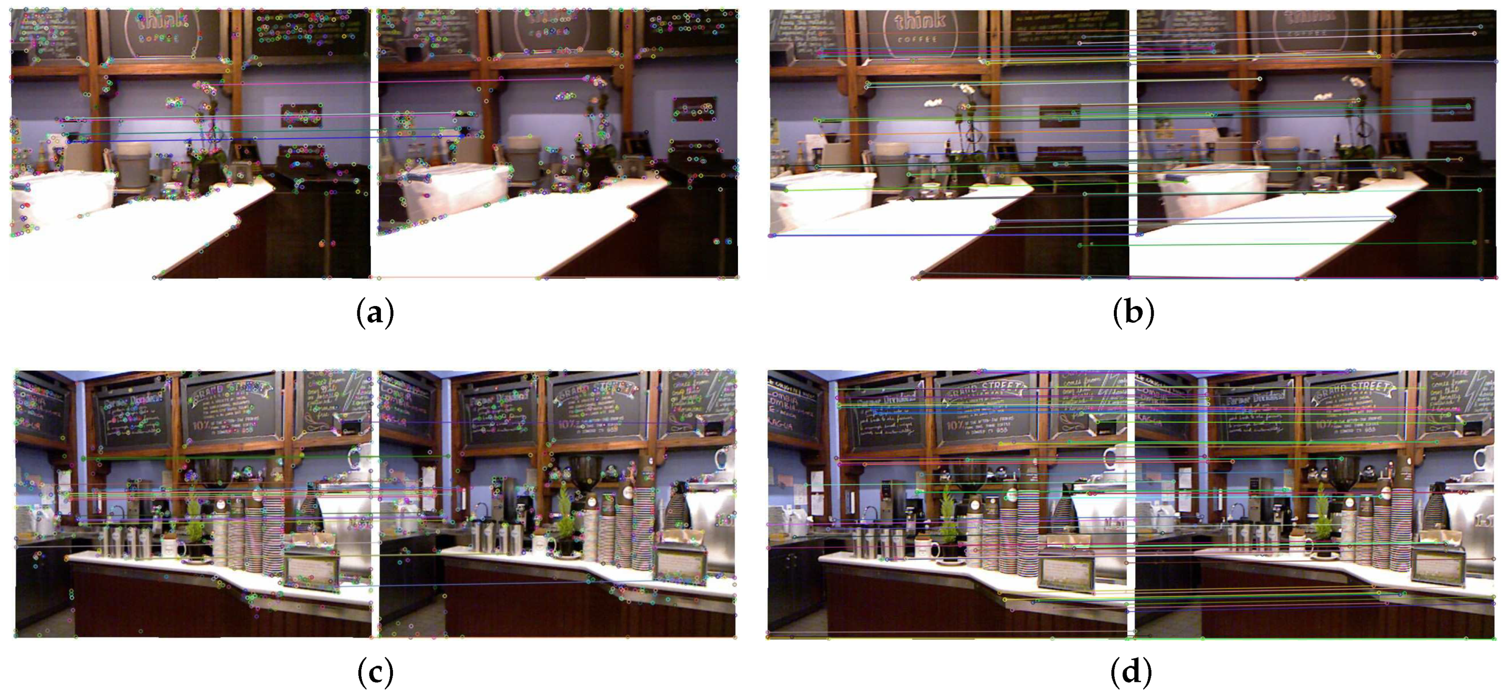
In this experiment, we compare the effect of the image segmentation into 16 cells and then extraction of the feature points with the effect of the overall extraction of feature points on the camera pose. Figure 7a,c show the feature points that are extracted from the whole image, and (b,d) show the images that are divided into 16 cells and then the feature points are extracted. By comparing (a) and (b), we find that after the image segmentation, the number of matching features is increased, and by comparing (c) and (d), we find that the distribution of the matching features is relatively uniform.

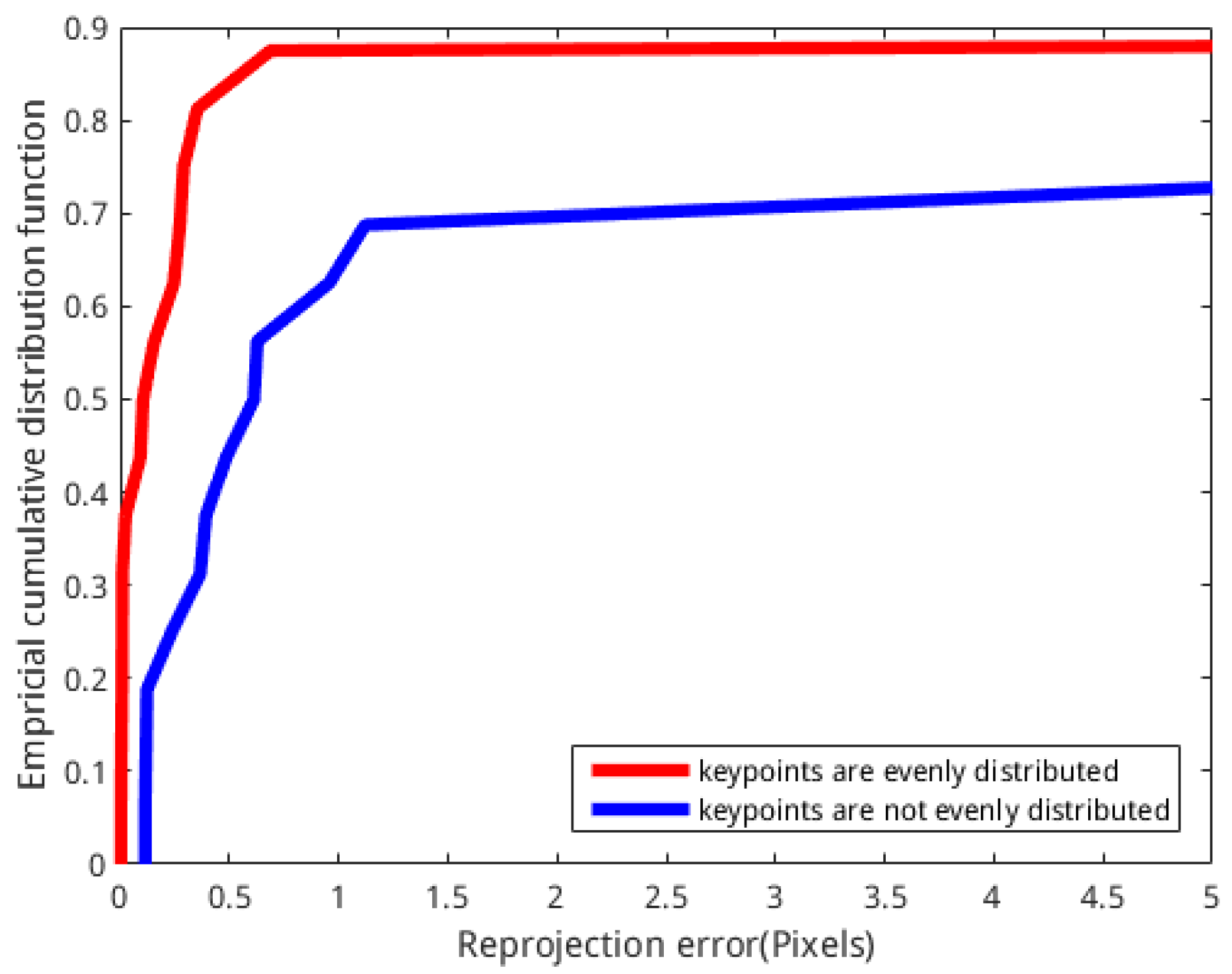
We calculated the reprojection error [44] and used the empirical cumulative distribution function to represent the quality of the camera pose, as shown in Figure 8. As shown in this figure, the reprojection error is clearly reduced when the feature points increase and distribute evenly. The detailed comparison of reprojection error is presented in

Table 3. Comparison of reprojection error.

	LUT-Based Method	Keyframe-Based Method
0.5 pixel reprojection error	84%	44%
50% cumulative probability	0.1 pixels	0.6 pixels

. This table shows that the cumulative probability is up to 84% for the LUT-based method when the reprojection error is 0.5, while that of the keyframe-based method is 44%. When the cumulative probability is 50%, the reprojection error based on the LUT method is 0.1 pixels, while that based on the keyframe-based method is 0.6 pixels. In other words, the relative pose error of the camera becomes smaller when the feature points increase and are evenly distributed.

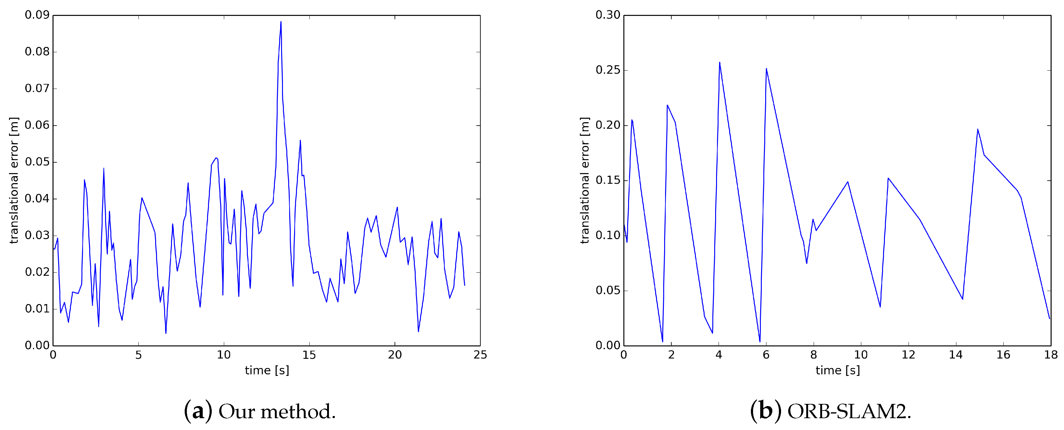
On the TUM dataset, we compute the relative pose error from the ground-truth trajectory and the trajectory estimated with the TUM automated evaluation tool and compare our method with the ORB-SLAM2 method. The translational error of the two methods on the TUM dataset is shown in Figure 9. The results of our method are significantly more intensive than ORB-SLAM2 because our keyframe strategy is simpler, with more keyframes being selected, and ORB-SLAM2 is almost one keyframe per second. The results show that our method runs longer than ORB-SLAM2 because ORB-SLAM2 has a longer initialization time and failed to track at the end of the data set. The translation error of our method is almost within 0.05, except that the maximum exceeds 0.08 but is less than 0.09, while the translation error of ORB-SLAM2 is between 0 and 0.25.

Table 4. Average translational error on the TUM dataset.

Mapping Method	Mean Translational Error
LUT-based	0.028 m
Keyframe-based	0.123 m

lists the average translational error, and we can find that the translational error of our method is clearly better than that of the ORB-SLAM2 method.

5.2. Estimating Moving Direction and Mapping with LUT

In this experiment, to estimate the camera movement direction, we subtract the coordinates of the matching feature points of the current frame from the coordinates of the feature points of the previous frame. Then, the parallax is compared with the threshold to determine which direction to move. As shown in Table 1, we can find the cell number needed for mapping. Then, we only update the information of these cells in the map. Figure 10 shows the result of our method. Through comparing Figure 2 and Figure 10, we find that the noise in the map built by the LUT-based method is reduced and the afterimages disappeared. However, the disadvantage is that the information on the left is incomplete. This is because in the situation of the far left, the left direction of movement only appeared once.

Table 5. Average time consumption.

Mapping Method	Time Consumption
Keyframe-based	4.88 s
LUT-based	1.46 s

shows the time consumption of the two mapping methods on the dataset (780 images). As shown, we use less than one-third of the time to build a better map with less noise.

5.3. Constructing Static Maps of Dynamic Scenes

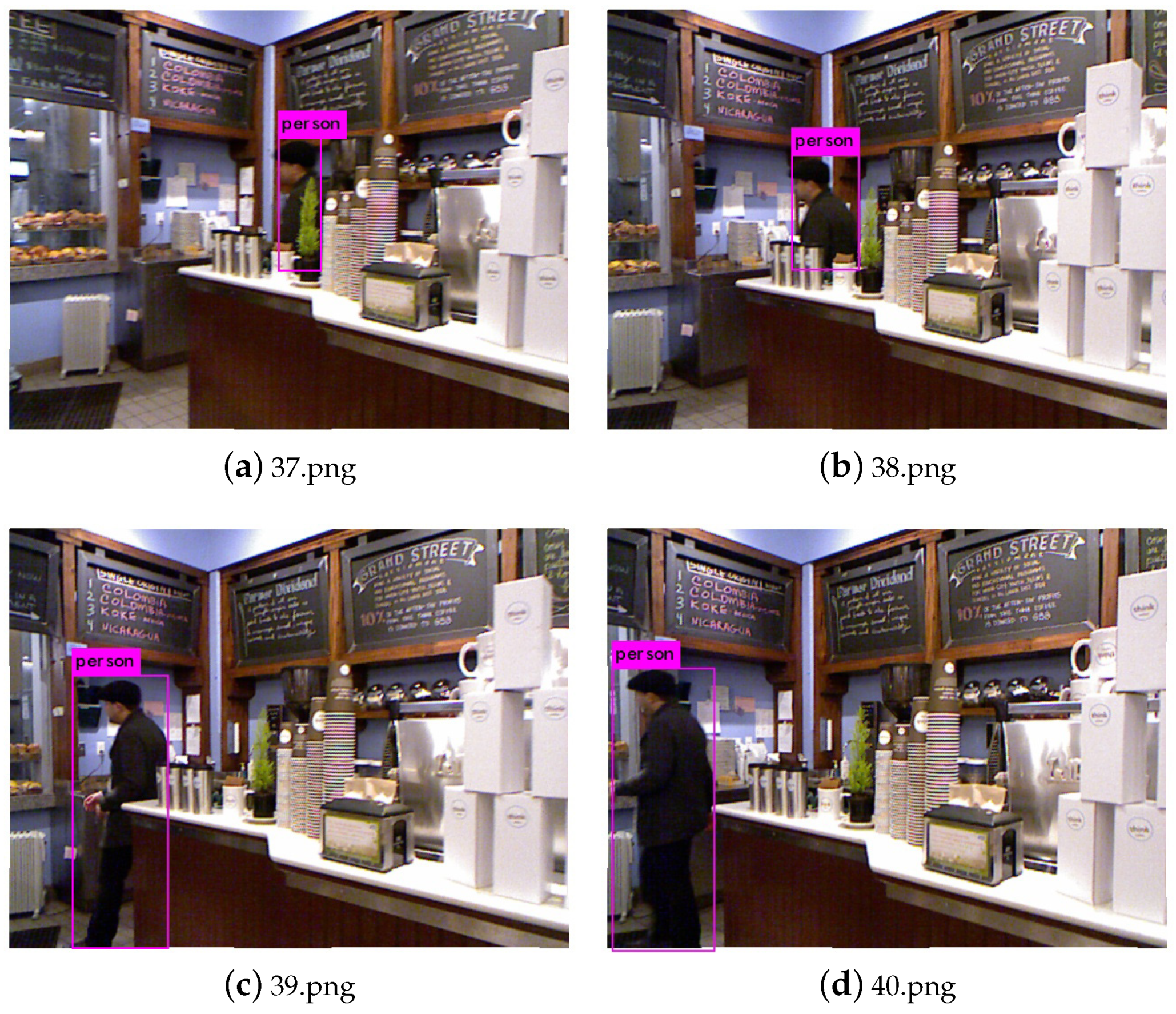
Although the afterimages of moving objects in the map have disappeared after the improvement of the SLAM mapping method based on lookup table, moving objects still appear in the map. To eliminate moving objects in the maps, i.e., to construct a static map in a dynamic scene, this section uses the YOLOv3 object detection network to detect the moving objects in the keyframe and then eliminates the moving object area in the process of SLAM to reduce the influence of the moving object on localization and mapping. Because the dynamic target in an indoor scene is generally only human, this experiment only uses the YOLOv3 network to detect the locations of persons in the image. As shown in Figure 11, the four keyframe images selected by the SLAM algorithm detect pedestrians in the scene after passing through the YOLOv3 object detection network.

Table 6. Average time consumption and detection probability.

Key-Frame Number	Time Consumption	Detection Probability
37.png	0.026546 s	96%
38.png	0.026966 s	100%
39.png	0.027040 s	100%
40.png	0.027665 s	100%
average	0.027054 s	99%

shows the time consumption of each image in the YOLOv3 network and the detection probability of a person. As shown, the YOLOv3 network takes an average of approximately 27 ms for each processed 640 × 480 image, and the accuracy rate of person detection is 99%.

Table 7. The pedestrian position coordinates.

Keyframe Number	Object Coordinates
37.png	307	355	148	297
38.png	212	288	167	296
39.png	76	184	169	475
40.png	11	126	161	478

shows the pedestrian position coordinates detected by the YOLOv3 network in four keyframes, which are represented by the upper left corner x coordinates of the detection frame, the upper left corner y coordinates, the lower right corner x coordinates and the lower right corner y coordinates in turn.

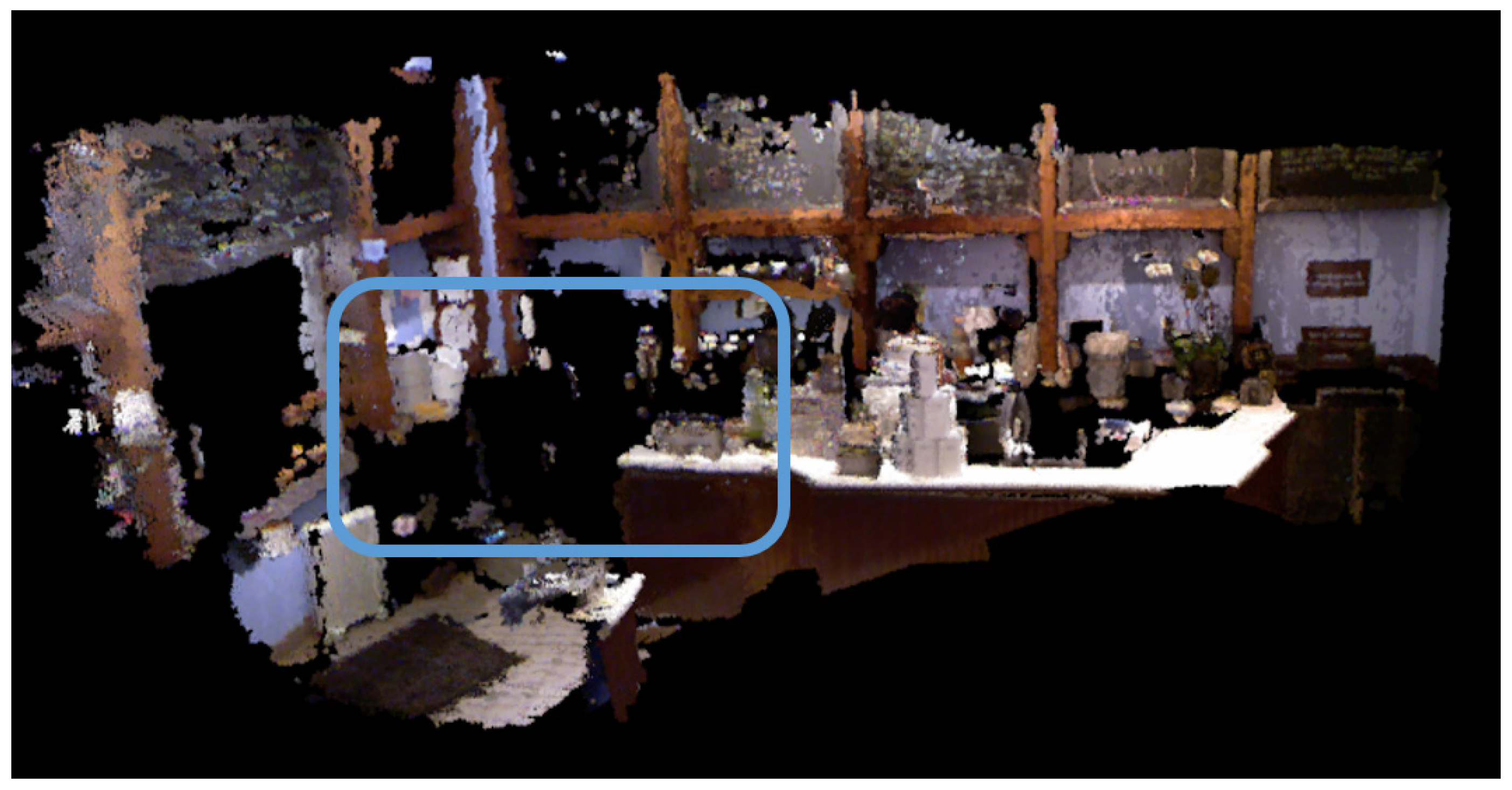
When the pedestrian position coordinates are available, pedestrians in the corresponding coordinate area can be removed on the basis of the lookup table to construct a static scene point cloud map. The experimental result of dynamic target rejection is shown in Figure 12. After comparison with Figure 2, it can be found that the pedestrians and afterimages in the scene have been eliminated.

5.4. Constructing Semantic Maps

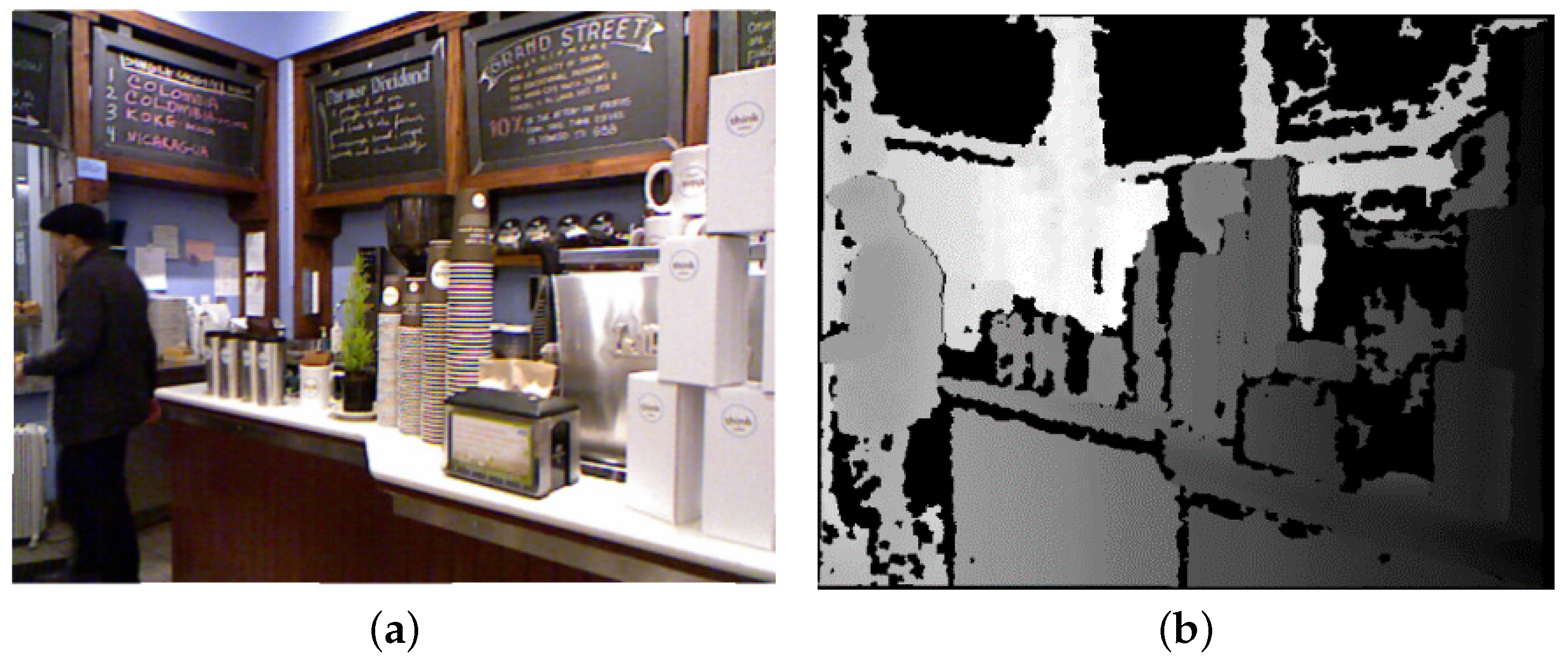
This section of the experiment was based on the previous experiment. Figure 13 shows the colour and depth images of the NYU Depth Dataset V2.

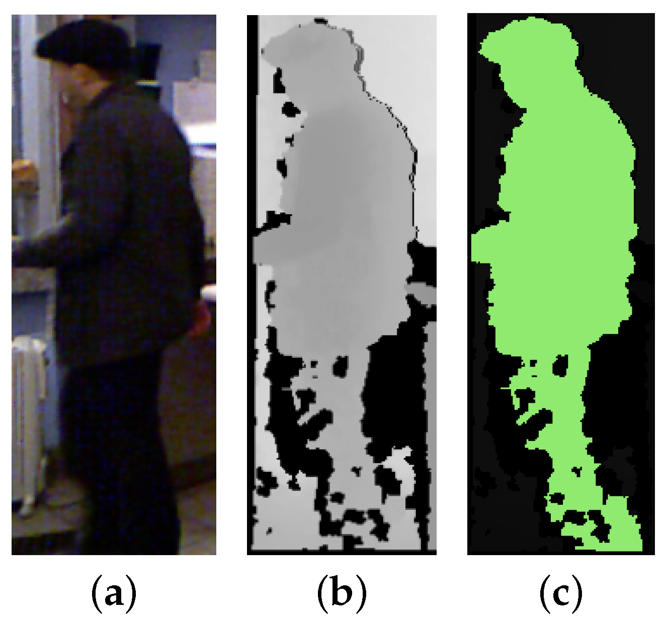
After the object detection experiment in Section 5.3, the area where the pedestrian is located in the colour image has been segmented, as shown in Figure 14a. The flood filling algorithm determines the connected area by the colour of the seed point. However, a single object in the scene does not necessarily have only one colour. For example, the colours of the face and hair of the pedestrian in Figure 14a are different, and more generally, the colours of the clothes worn by people may also vary. To solve this problem, this paper chooses to implement the depth map-based flood filling algorithm on the depth image. Because the depth image is a grayscale image and the depth of the same object is generally not much different, the flood filling algorithm on the depth map can avoid the problem that the same object has different colours. Figure 14b shows the segmentation result of the target detection area on the depth map, and the effect map after flood filling is shown in Figure 14c. As shown, the human body in the depth map has been well marked. The holes in pedestrian legs are caused by the error of the depth map, which has little influence on the overall pedestrian object detection and semantic segmentation.

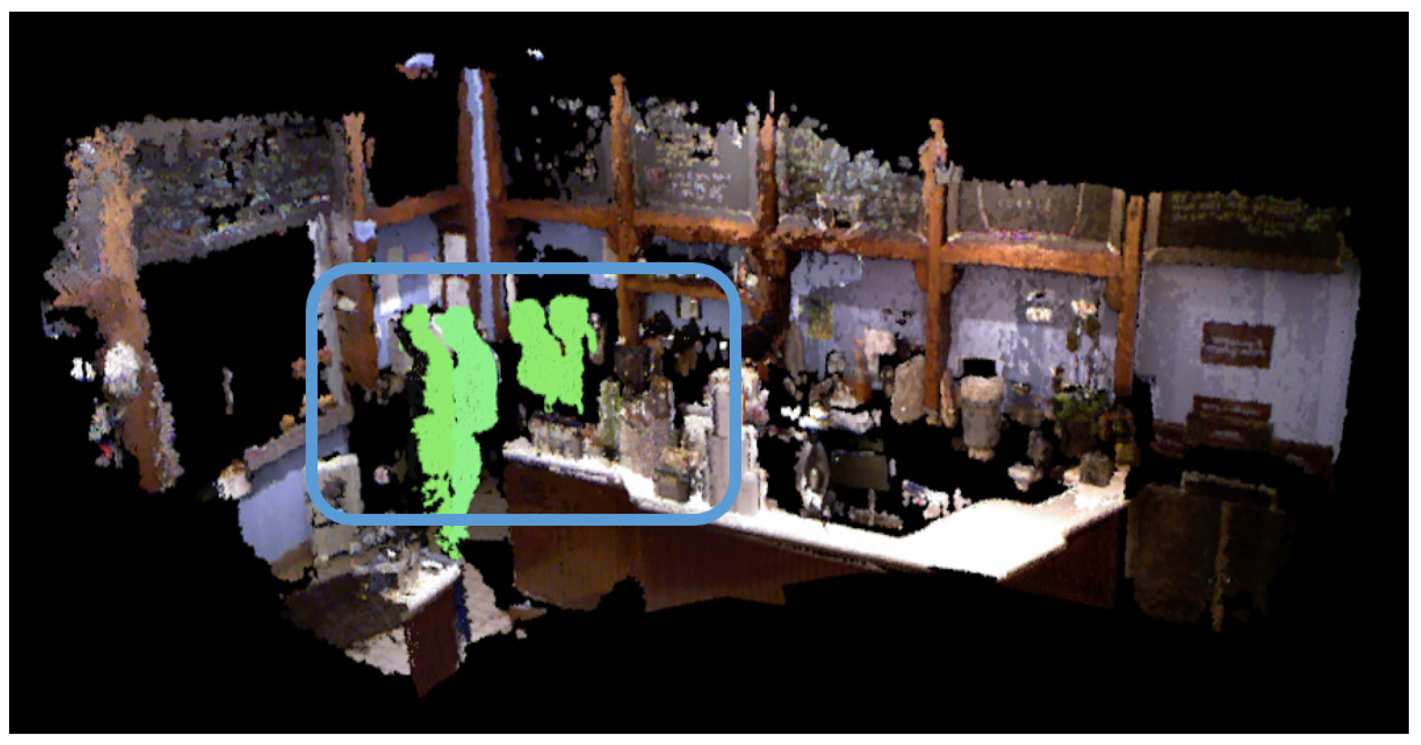
Next, semantic tags are added to the SLAM system to obtain a scene point cloud map with partial semantic information, as shown in Figure 15. As shown, the pedestrians in the keyframe are clearly marked in the map, which is a good representation of the pedestrian trajectory. Compared to the various semantic segmentation methods based on deep learning shown in Figure 3, our method can segment specific targets with high-precision in real time.

As shown in

Table 8. Segmentation accuracy of depth map-based flood filling method.

Images	Number of Pedestrian Pixels
Figure 14b	16,076
Figure 14c	16,714
intersection of (b) and (c)	16,010
union of (b) and (c)	16,780
intersection over union (IoU)	95.41%

, we counted the number of pedestrian pixels in Figure 14b,c, respectively, and then we calculated their intersection, union and intersection over union (IoU). As shown, the IoU segmentation accuracy of our method can reach 95.41%. Using the same method to statistics the whole NYU Depth Dataset V2, the ratio reaches 95.2%, which is far higher than the accuracy of semantic segmentation of PSPNet network (81%).

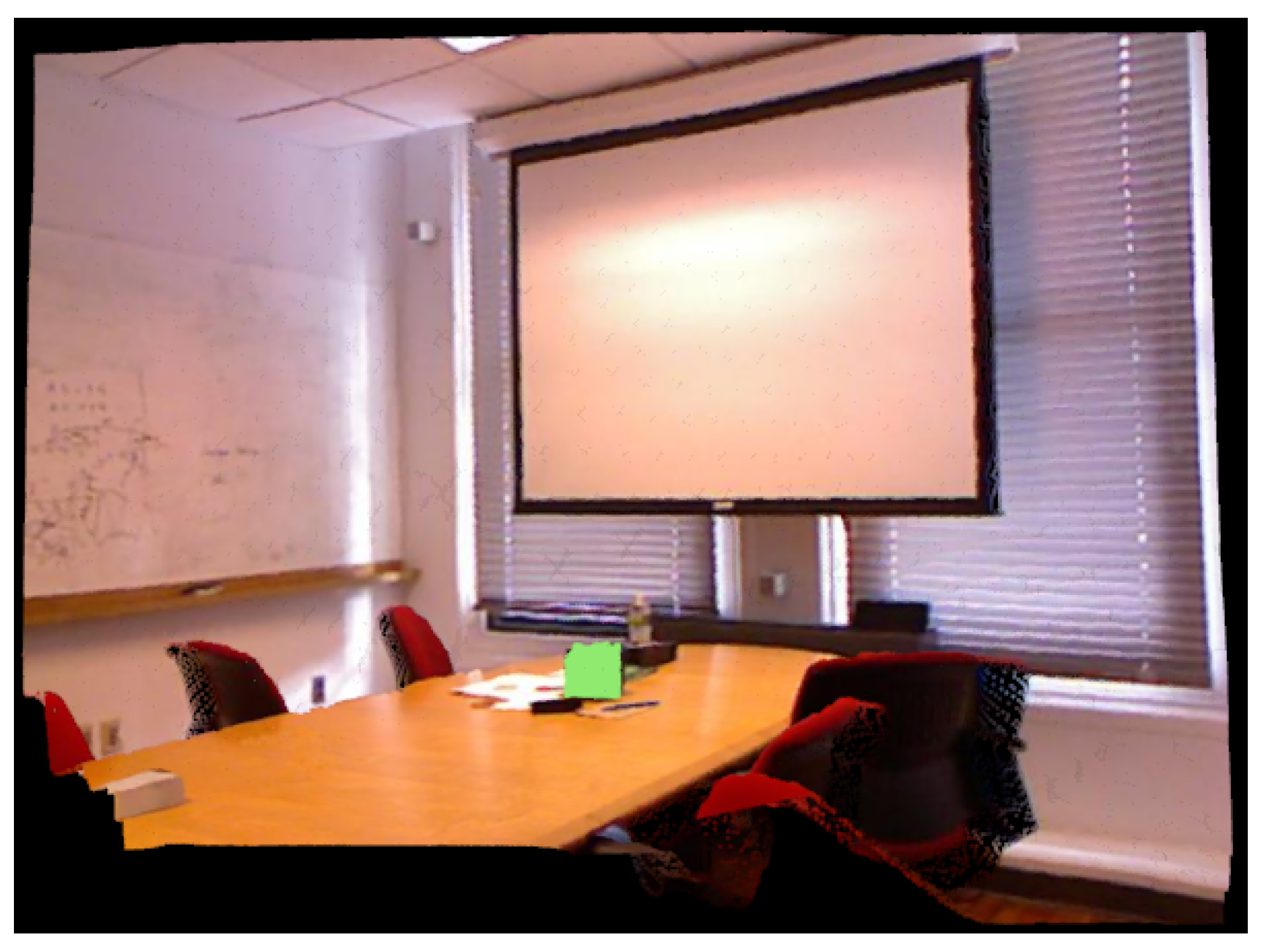
In addition tracking and marking pedestrians in scenes, it can also be used for other robot tasks, such as picking up cups on a table, throwing trash into a trash can, and so on. As shown in Figure 16, a cup on a table was marked, and this will provide useful help for the robot’s task execution. Moreover, in addition to marking a single object in the scene, our system also supports multiple specific objects to provide conditions for complex applications of robots.

6. Conclusions

In this paper, we present a computationally efficient solution of semantic SLAM, which is applicable for dynamic scenes containing moving objects. On the one hand, the proposed solution incorporates a deep learning method with LUT-based SLAM, and it detects and recognizes specific moving objects using the deep learning method YOLOv3; correspondingly, these moving objects are removed from the point cloud maps of scenes in the process of SLAM. Consequently, the localization accuracy and the quality of the generated maps are improved compared to established SLAM methods. On the other hand, in contrast to traditional semantic SLAM methods, which obtain semantic information by using semantic segmentation networks that are computationally intensive and where the segmentation results are not very accurate, the proposed solution replaces semantic segmentation networks with object detection networks and depth map-based flood filling algorithms. As a result, it can obtain high-precision semantic information of specific objects in real time. Finally, the proposed solution is able to generate static geometric map of a scene, as well as a semantic map including semantic information of moving objects.

The experiments show that the proposed solution is very efficient in building maps; it can construct a better quality map in one-third of the time of the traditional method. Its relative pose accuracy is an order of magnitude higher than that of ORB-SLAM2. The relative translation error of ORBSLAM2 on the TUM dataset is 0.123 m, while ours is only 0.028 m. In addition, its semantic segmentation is highly accurate and fast. The traditional semantic segmentation method has the highest accuracy of only 81%, and the processing speed is 1.5 FPS. However, the segmentation accuracy of our method can reach more than 95%, and the running speed can reach 35 FPS. Moreover, it is not interfered by moving objects, can run in a dynamic scene, generate static maps of dynamic scenes and semantic maps with high-precision semantic information of specific objects in real time.

Our solution is applicable for real-time intelligent systems such as mobile robots. In the future, we will explore the use of semantic information to constrain the tracking process, further improving the accuracy and robustness of localization. In addition, the moving objects do have a significant impact on loop closure, whether the strategy of loop detection is matching feature points or Bag of Words(DBOW2) [10]. In theory, this problem can be solved by removing the moving objects in the original data before the loop detection, or using a semantic-based loop detection strategy, and we plan to conduct a further study in the future.

References

- Liu, J.; Chen, R.; Chen, Y.; Pei, L.; Chen, L. iParking: An Intelligent Indoor Location-Based Smartphone Parking Service. Sensors 2012, 12, 14612–14629. [Google Scholar] [CrossRef]
- Smith, R.C.; Cheeseman, P. On the representation and estimation of spatial uncertainty. Int. J. Robot. Res. 1986, 5, 56–68. [Google Scholar] [CrossRef]
- Tan, W.; Liu, H.; Dong, Z.; Zhang, G.; Bao, H. Robust monocular SLAM in dynamic environments. In Proceedings of the IEEE International Symposium on Mixed and Augmented Reality (ISMAR), Adelaide, Australia, 1–4 October 2013. [Google Scholar]
- Agudo, A.; Moreno-Noguer, F.; Calvo, B.; Martínez, J.M. Sequential non-rigid structure from motion using physical priors. IEEE Trans. Pattern Anal. Mach. Intell. 2016, 38, 979–994. [Google Scholar] [CrossRef] [PubMed]
- Agudo, A.; Moreno-Noguer, F.; Calvo, B.; Martínez, J.M. Real-time 3D reconstruction of non-rigid shapes with a single moving camera. Comput. Vis. Image Underst. 2016, 153, 37–54. [Google Scholar] [CrossRef] [Green Version]
- Liu, J.; Chen, R.; Pei, L.; Guinness, R.; Kuusniemi, H. A hybrid smartphone indoor positioning solution for mobile LBS. Sensors 2012, 12, 17208–17233. [Google Scholar] [CrossRef] [PubMed]
- Liu, J.; Zhu, L.; Wang, Y.; Liang, X.; Hyyppä, J.; Chu, T.; Liu, K.; Chen, R. Reciprocal Estimation of Pedestrian Location and Motion State toward a Smartphone Geo-Context Computing Solution. Micromachines 2015, 6, 699–717. [Google Scholar] [CrossRef] [Green Version]
- Strasdat, H.; Davison, A.J.; Montiel, J.M.; Konolige, K. Double window optimisation for constant time visual SLAM. In Proceedings of the 2011 International Conference on Computer Vision, Barcelona, Spain, 6–13 November 2011; Volume 58, pp. 2352–2359. [Google Scholar]
- Klein, G.; Murray, D. Parallel Tracking and Mapping for Small AR Workspaces. In Proceedings of the IEEE and ACM International Symposium on Mixed and Augmented Reality, Nara, Japan, 13–16 November 2007; pp. 1–10. [Google Scholar]
- Mur-Artal, R.; Montiel, J.M.M.; Tardós, J.D. A Versatile and Accurate Monocular SLAM System. IEEE Trans. Robot. 2015, 31, 1147–1163. [Google Scholar] [CrossRef]
- Engel, J.; Koltun, V.; Cremers, D. Direct Sparse Odometry. IEEE Trans. Pattern Anal. Mach. Intell. 2016, 99, 1–10. [Google Scholar] [CrossRef] [PubMed]
- Nüchter, A.; Hertzberg, J. Towards semantic maps for mobile robots. Robot. Auton. Syst. 2008, 56, 915–926. [Google Scholar] [CrossRef] [Green Version]
- Bao, S.Y.; Savarese, S. Semantic Structure from Motion: A Novel Framework for Joint Object Recognition and 3D Reconstruction; Springer: Berlin/Heidelberg, Germany, 2012; pp. 376–397. [Google Scholar]
- Salas-Moreno, R.F.; Newcombe, R.A.; Strasdat, H.; Kelly, P.H.J.; Davison, A.J. SLAM++: Simultaneous Localisation and Mapping at the Level of Objects. In Proceedings of the IEEE Conference on Computer Vision and Pattern Recognition, Portland, OR, USA, 23–28 June 2013; pp. 1352–1359. [Google Scholar]
- Salas-Moreno, R.F.; Glocker, B.; Kelly, P.H.J.; Davison, A.J. Dense planar SLAM. In Proceedings of the IEEE International Symposium on Mixed and Augmented Reality, Munich, Germany, 10–12 September 2014; pp. 367–368. [Google Scholar]
- Vineet, V.; Miksik, O.; Lidegaard, M.; Nießner, M.; Golodetz, S.; Prisacariu, V.A.; Kähler, O.; Murray, D.W.; Izadi, S.; Pérez, P.; et al. Incremental dense semantic stereo fusion for large-scale semantic scene reconstruction. In Proceedings of the IEEE International Conference on Robotics and Automation, Seattle, WA, USA, 26–30 May 2015; pp. 75–82. [Google Scholar]
- Mccormac, J.; Handa, A.; Davison, A.; Leutenegger, S. SemanticFusion: Dense 3D Semantic Mapping with Convolutional Neural Networks. In Proceedings of the IEEE International Conference on Robotics and Automation (ICRA), Columbus, OH, USA, 29 May–3 June 2017; pp. 4628–4635. [Google Scholar]
- Zhao, H.; Shi, J.; Qi, X.; Wang, X.; Jia, J. Pyramid Scene Parsing Network. arXiv 2017, arXiv:1612.01105. [Google Scholar]
- Adam, P.; Abhishek, C.; Sangpil, K.; Eugenio, C. ENet: A Deep Neural Network Architecture for Real-Time Semantic Segmentation. arXiv 2016, arXiv:1606.02147. [Google Scholar]
- Zhao, H.; Qi, X.; Shen, X.; Shi, J.; Jia, J. ICNet for Real-Time Semantic Segmentation on High-Resolution Images. arXiv 2017, arXiv:1704.08545. [Google Scholar]
- Long, J.; Shelhamer, E.; Darrell, T. Fully convolutional networks for semantic segmentation. In Proceedings of the 2015 IEEE Conference on Computer Vision and Pattern Recognition (CVPR), Boston, MA, USA, 7–12 June 2015. [Google Scholar]
- Chen, L.; Papandreou, G.; Kokkinos, I.; Murphy, K.; Yuille, A.L. Semantic image segmentation with deep convolutional nets and fully connected crfs. arXiv 2015, arXiv:1412.7062. [Google Scholar]
- Badrinarayanan, V.; Kendall, A.; Cipolla, R. Segnet: A deep convolutional encoder-decoder architecture for image segmentation. IEEE Trans. Pattern Anal. Mach. Intell. 2017, 39, 2481–2495. [Google Scholar] [CrossRef]
- Wu, Z.; Shen, C.; van den Hengel, A. Wider or deeper: Revisiting the resnet model for visual recognition. arXiv 2016, arXiv:1611.10080. [Google Scholar] [CrossRef]
- Lin, G.; Milan, A.; Shen, C.; Reid, I.D. Refinenet: Multi-path refinement networks for high-resolution semantic segmentation. arXiv 2017, arXiv:1611.06612. [Google Scholar]
- Chen, L.; Papandreou, G.; Kokkinos, I.; Murphy, K.; Yuille, A.L. Deeplab: Semantic image segmentation with deep convolutional nets, atrous convolution, and fully connected crfs. arXiv 2018, arXiv:1606.00915. [Google Scholar] [CrossRef]
- Liu, Z.; Li, X.; Luo, P.; Loy, C.C.; Tang, X. Semantic image segmentation via deep parsing network. arXiv 2015, arXiv:1509.02634. [Google Scholar]
- Zheng, S.; Jayasumana, S.; Romera-Paredes, B.; Vineet, V.; Su, Z.; Du, D.; Huang, C.; Torr, P.H.S. Conditional random fields as recurrent neural networks. arXiv 2015, arXiv:1502.03240. [Google Scholar]
- Girshick, R.; Donahue, J.; Darrell, T.; Malik, J. Rich Feature Hierarchies for Accurate Object Detection and Semantic Segmentation. In Proceedings of the IEEE Conference on Computer Vision and Pattern Recognition (CVPR), Singapore, 24–27 June 2014. [Google Scholar]
- Girshick, R. Fast R-CNN. In Proceedings of the IEEE International Conference on Computer Vision (ICCV), Santiago, Chile, 7–13 December 2015. [Google Scholar]
- Ren, S.; He, K.; Girshick, R.; Sun, J. Faster R-CNN: Towards Real-Time Object Detection with Region Proposal Networks. arXiv 2015, arXiv:1506.01497. [Google Scholar] [CrossRef]
- He, K.; Gkioxari, G.; Dollár, P.; Girshick, R. Mask R-CNN. In Proceedings of the IEEE International Conference on Computer Vision (ICCV), Venice, Italy, 22–29 October 2017. [Google Scholar]
- Liu, W.; Anguelov, D.; Erhan, D.; Szegedy, C.; Reed, S.; Fu, C.; Berg, A.C. SSD: Single Shot MultiBox Detector. arXiv 2016, arXiv:1512.02325. [Google Scholar]
- Redmon, J.; Divvala, S.; Girshick, R.; Farhadi, A. You Only Look Once: Unified, Real-Time Object Detection. arXiv 2015, arXiv:1506.02640. [Google Scholar]
- Redmon, J.; Divvala, S.; Girshick, R.; Farhadi, A. YOLO9000: Better, Faster, Stronger. arXiv 2016, arXiv:1612.08242. [Google Scholar]
- Redmon, J.; Divvala, S.; Girshick, R.; Farhadi, A. YOLOv3: An Incremental Improvement. arXiv 2018, arXiv:1804.02767. [Google Scholar]
- Lowe, D.G. Object Recognition from Local Scale-Invariant Features. In Proceedings of the Seventh IEEE International Conference on Computer Vision, Kerkyra, Greece, 20–27 September 1999. [Google Scholar]
- Lowe, D.G. Distinctive Image Features from Scale-Invariant Keypoints. Int. J. Comput. Vis. 2004, 60, 91–110. [Google Scholar] [CrossRef]
- Rublee, E.; Rabaud, V.; Konolige, K.; Bradski, G. ORB: An efficient alternative to SIFT or SURF. Int. Conf. Comput. Vis. 2012, 58, 2564–2571. [Google Scholar]
- Lepetit, V.; Moreno-Noguer, F.; Fua, P. Accurate O(n) solution to the PnP problem. Int. J. Comput. Vis. 2009, 81, 155–166. [Google Scholar] [CrossRef]
- Fischler, M.A.; Bolles, R.C. Random Sample Consensus: A Paradigm for Model Fitting with Applications to Image Analysis and Automated Cartography. Commun. ACM 1981, 24, 381–3950. [Google Scholar] [CrossRef]
- Triggs, B.; McLauchlan, P.; Hartley, R.; Fitzgibbon, A. Bundle Adjustment—A Modern Synthesis. In Proceedings of the International Workshop on Vision Algorithms(ICCV), Corfu, Greece, 20–25 September 1999; pp. 298–372. [Google Scholar]
- Kuemmerle, R.; Grisetti, G.; Strasdat, H.; Konolige, K.; Burgard, W. A General Framework for Graph Optimization. IEEE Int. Conf. Robot. Autom. (ICRA) 2011, 7, 3607–3613. [Google Scholar]
- Hartley, R. Camera geometry and single view geometry. In Multiple View Geometry in Computer Vision; Cambridge University Press: New York, NY, USA, 2003; pp. 153–158. [Google Scholar]
- Nathan, S.; Derek, H.; Pushmeet, K.; Rob, F. Indoor Segmentation and Support Inference from RGBD Images. IEEE ECCV 2012, 7576, 746–760. [Google Scholar]
- Sturm, J.; Engelhard, N.; Endres, F.; Burgard, W.; Cremers, D. A Benchmark for the Evaluation of RGB-D SLAM Systems. In Proceedings of the IEEE the International Conference on Intelligent Robot Systems (IROS), Vilamoura, Algarve, 7–12 October 2012. [Google Scholar]
Figure 1.
Several keyframe images selected by the traditional visual SLAM system are almost the same, which brings redundant information when constructing maps and reduces the efficiency of mapping.
Figure 2.
Dense point cloud map constructed by keyframe-based SLAM. We can find that pedestrians in the scene also appear in the map, which will bring many difficulties to the application of the map, such as path planning.
Figure 3.
Inference speed and mean intersection over union (mIoU) of mainstream semantic segmentation networks: PSPNet [18], ENet [19], ICNet [20], FCN-8s [21], DeepLab [22], SegNet [23], ResNet38 [24], RefineNet [25], DeepLabv2-CRF [26], DPN [27], and CRF-RNN [28]. These methods have difficultly in balancing the accuracy and speed of segmentation.
Figure 4.
The overview of the proposed solution.
Figure 5.
Bounding boxes with dimension priors and location prediction. The width and height of the box as offsets from cluster centroids and the centre coordinates of the box relative to the location of filter application are predicted.
Figure 6.
The image is divided equally into 16 cells and the eight-neighbourhood direction of the image.
Figure 7.
(a,c) extract feature points in the whole image, (b,d) divide the image equally into 16 cells and extract feature points in every cell. We find that the feature points in (b,d) are significantly more than (a,c), and the feature points are more evenly distributed. (a) Extract feature points in whole image, and good match condition is 5 times the minimum distance. (b) Divide image equally into 16 cells and extract feature points. (c) Extract feature points in whole image, and good match condition is 5 times the minimum distance. (d) Divide image equally into 16 cells and extract feature points.
Figure 8.
The empirical cumulative distribution function of the reprojection error.
Figure 9.
Translational error on the TUM dataset.
Figure 10.
Dense point cloud map constructed by our method.
Figure 11.
Object detection result of YOLOv3 network.
Figure 12.
Static map of dynamic scenes.
Figure 13.
NYU Depth Dataset V2. (a) shows the colour image, and (b) shows the depth image.
Figure 14.
Extract pedestrian contours. (a) shows the area where the pedestrian is located in the colour image, (b) shows the area where the pedestrian is located in the depth image, and (c) shows the effect map after the depth map-based flood filling.
Figure 15.
Pedestrian trajectory in static maps. The green pedestrian labels from right to left in the figure are the positions of pedestrians at times 1–4.
Figure 16.
A cup on a table.