An Integrated View of Greenland Ice Sheet Mass Changes Based on Models and Satellite Observations

 , , , , , , , ,
Abstract
:1. Introduction
2. Methods and Datasets
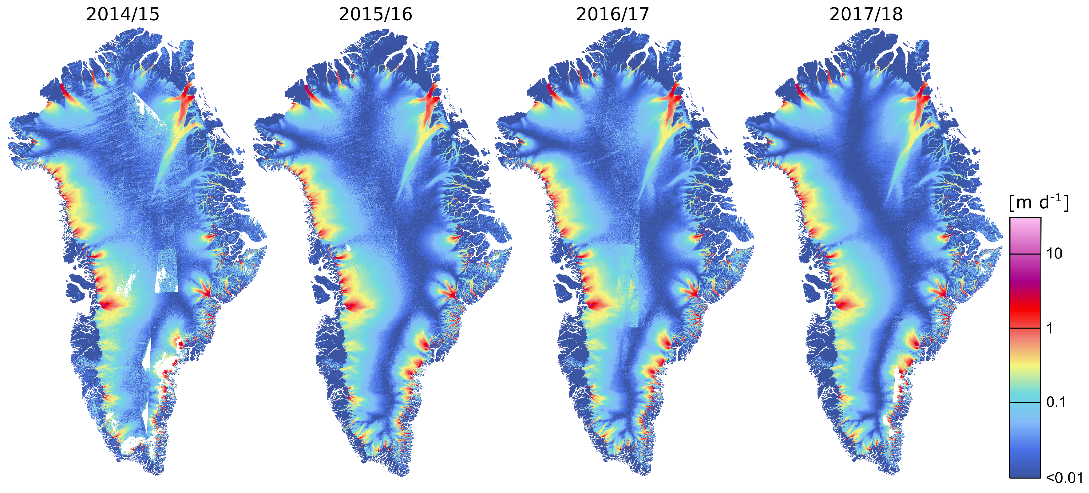
2.1. Ice Velocity
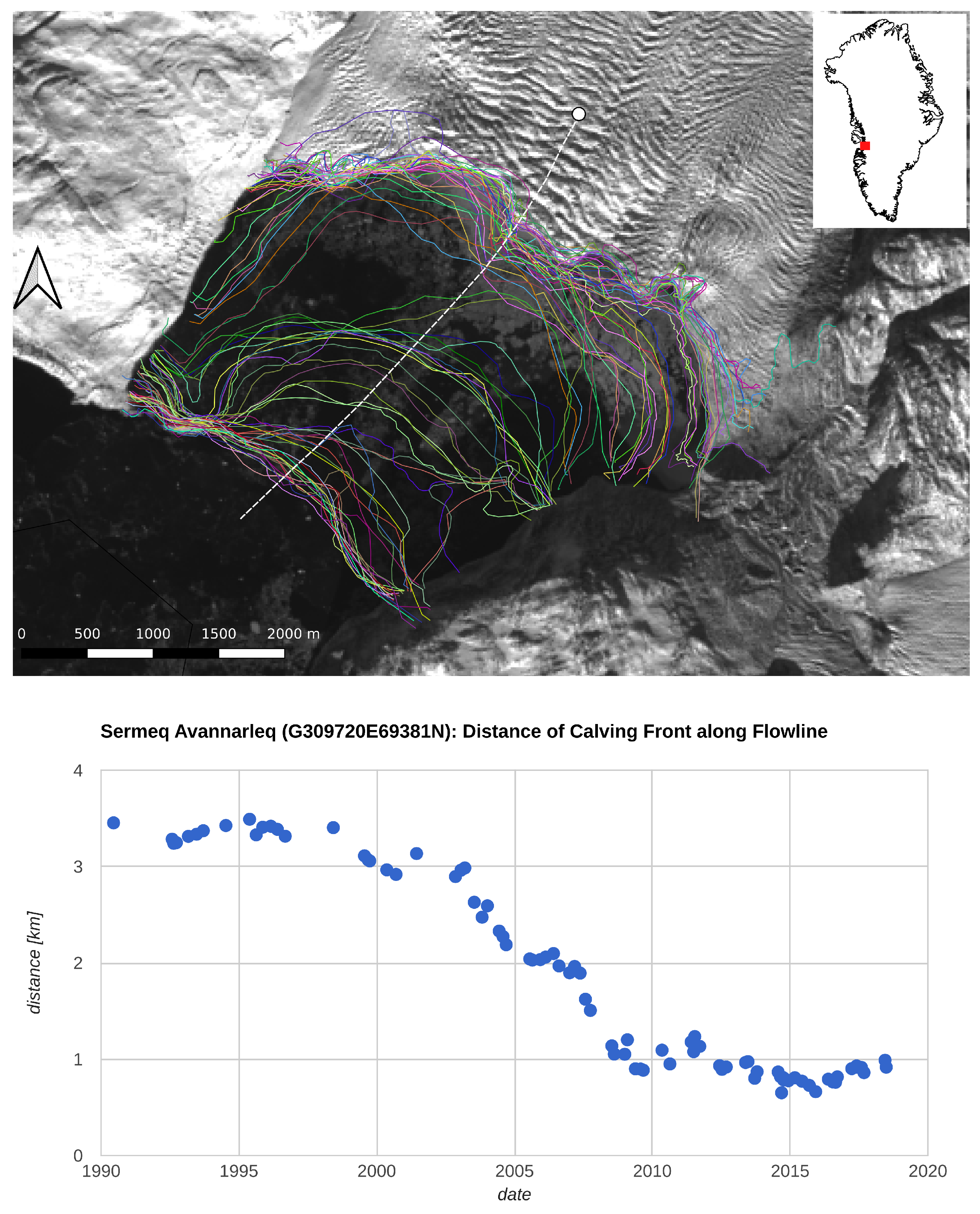
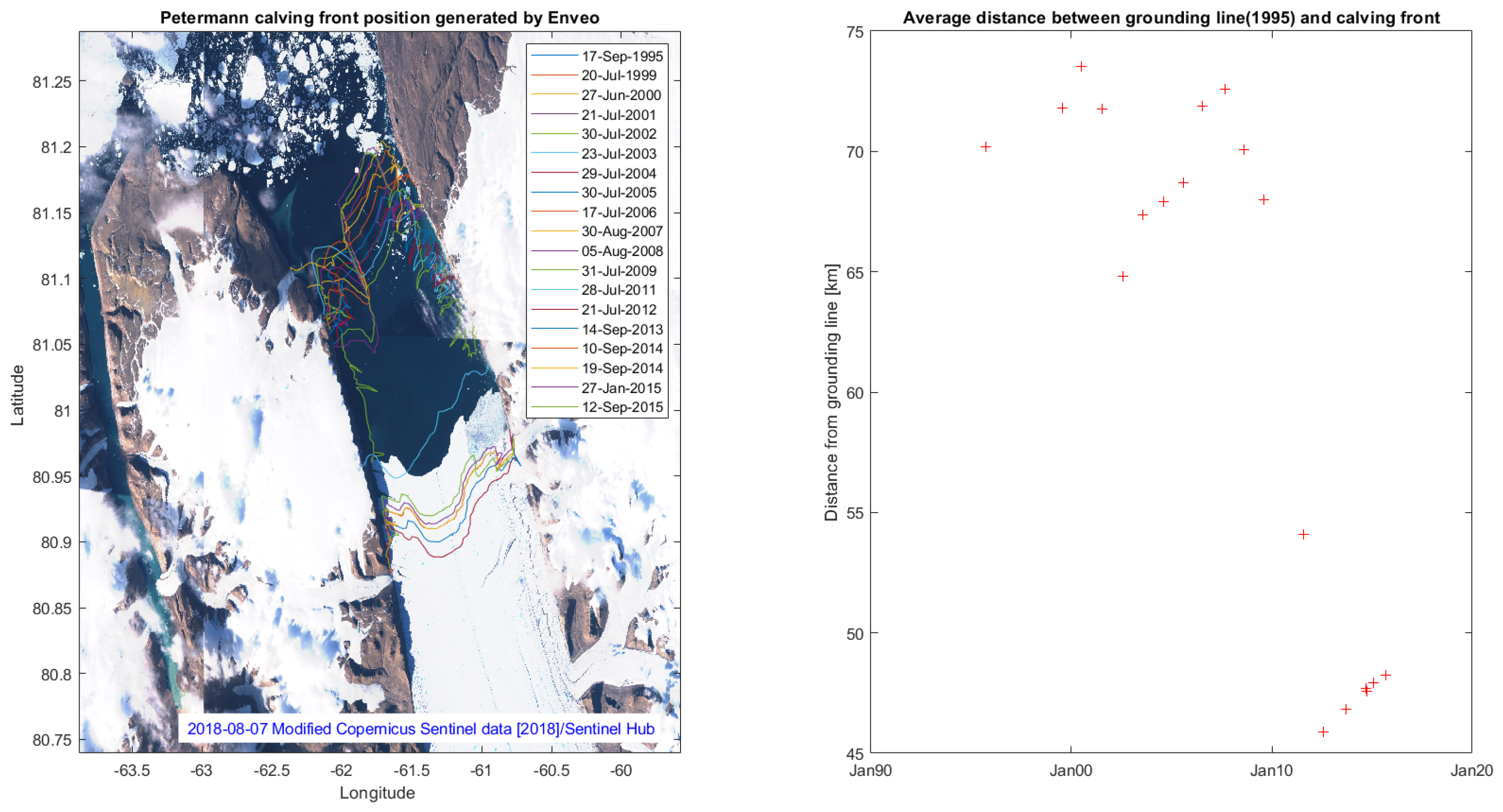
2.2. Calving Fronts
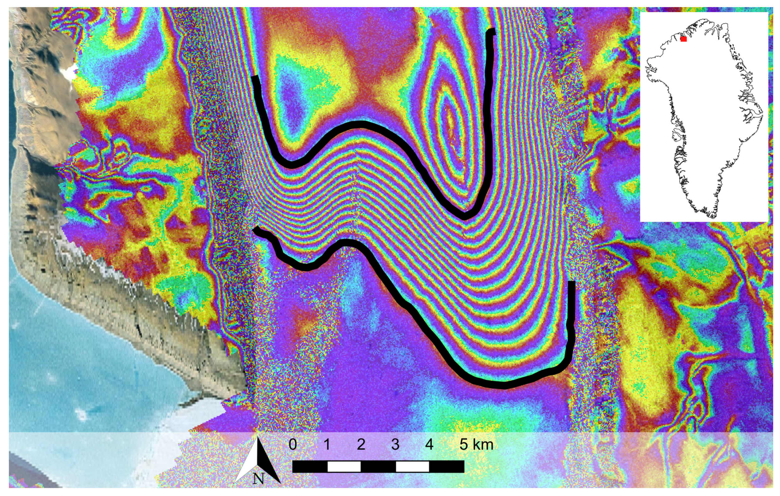
2.3. Grounding Lines
2.4. Surface Elevation Change
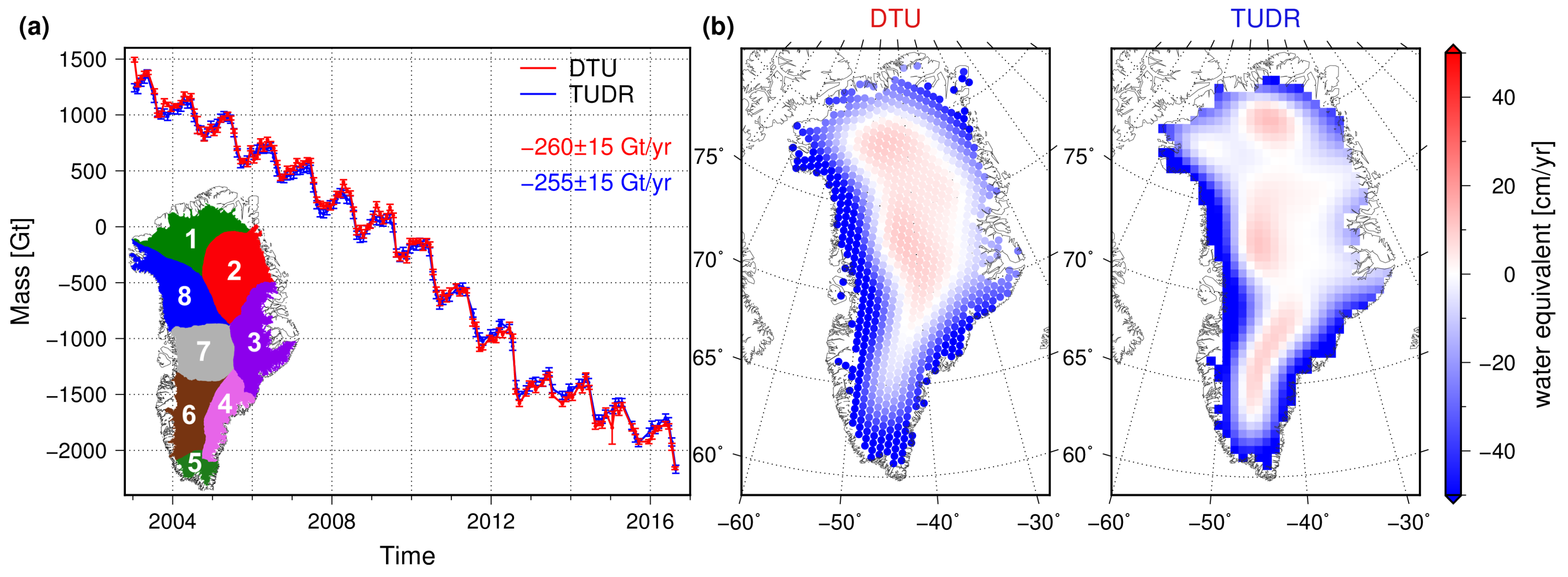
2.5. Gravimetric Mass Balance from GRACE
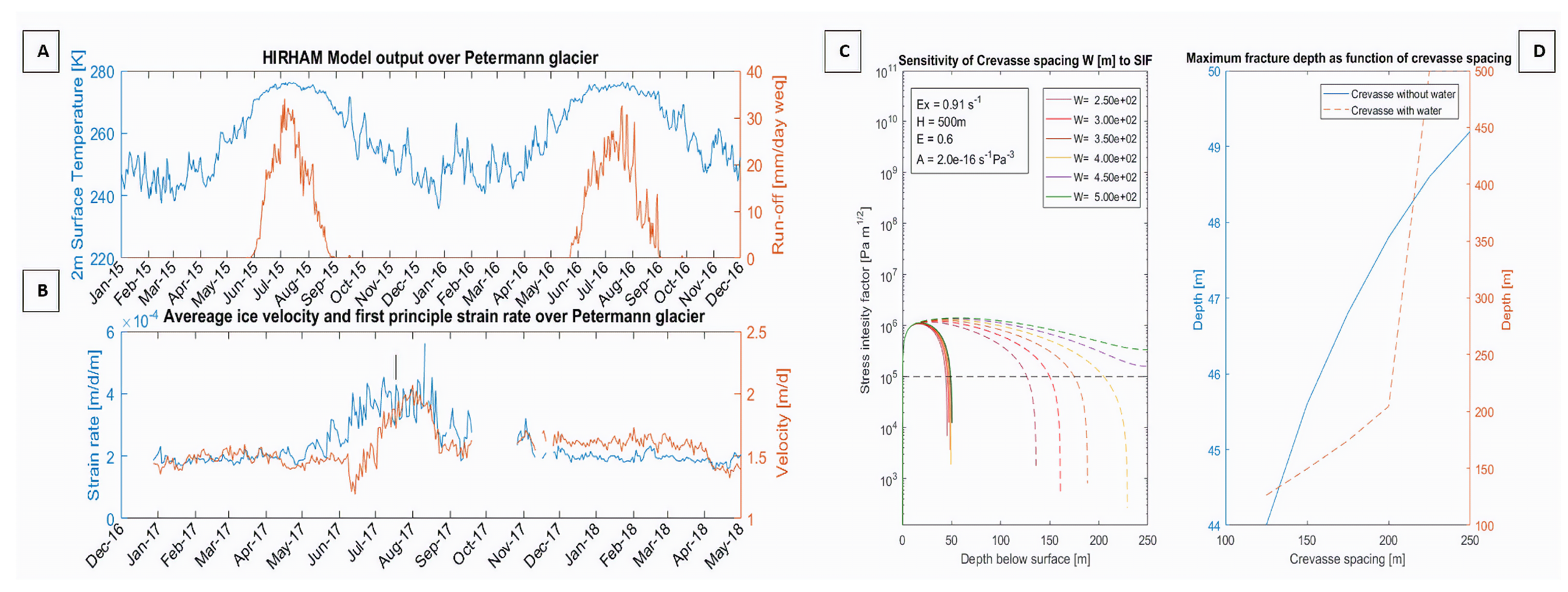
2.6. Regional Climate Model HIRHAM5
2.7. Ice Sheet Modelling with PISM
3. Results and Discussion
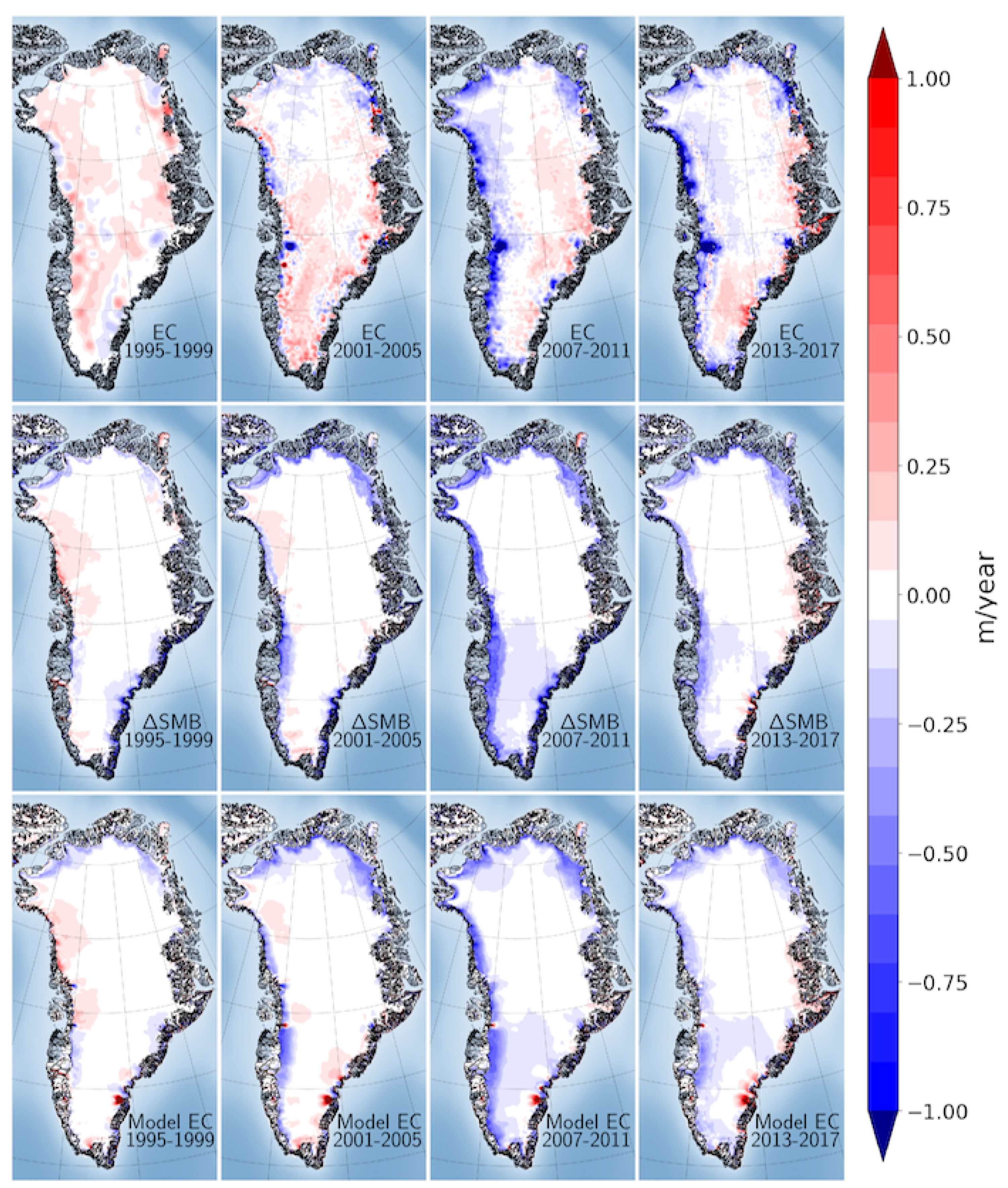
3.1. Surface Elevation Change in Models and Observations
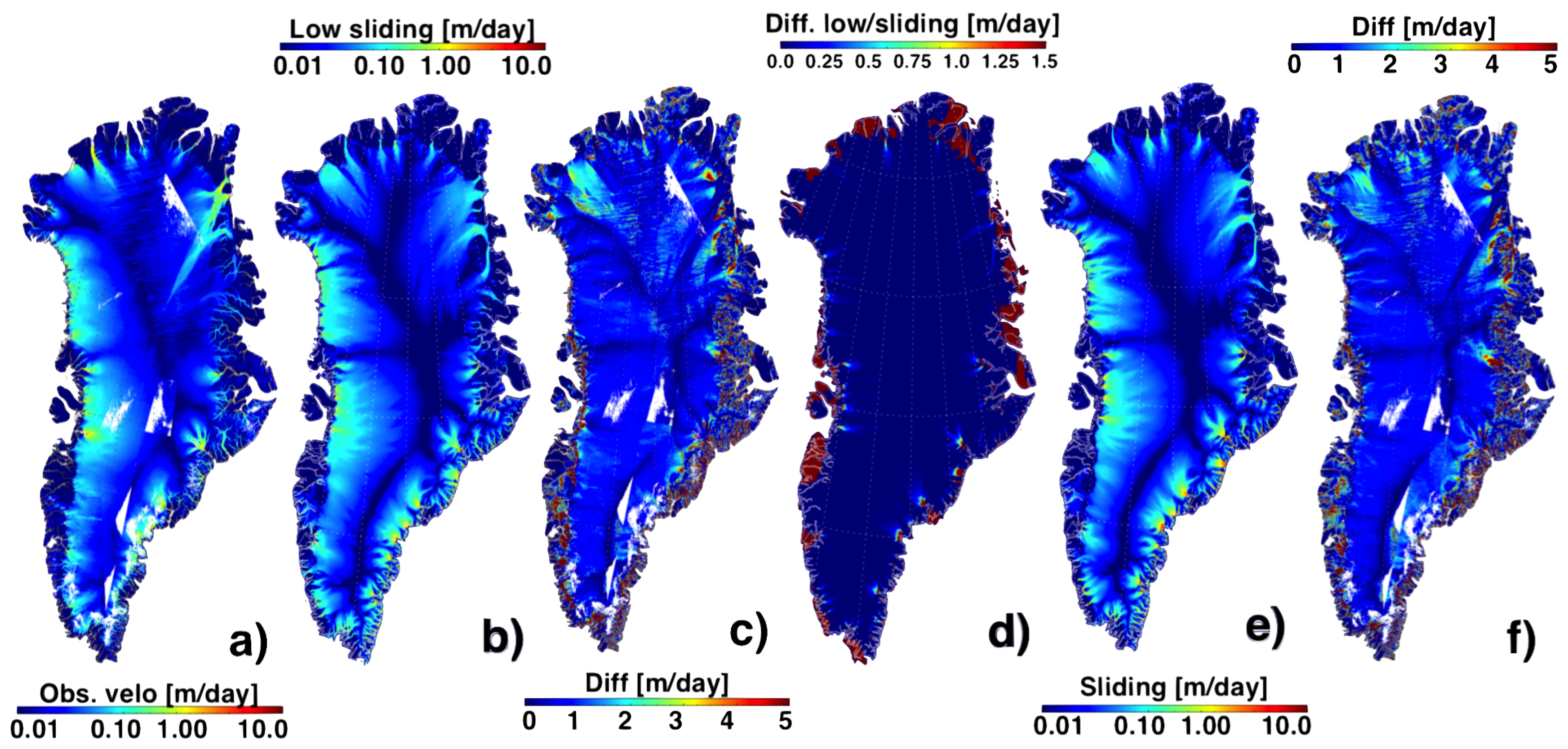
3.2. Modelled and Observed Ice Velocities
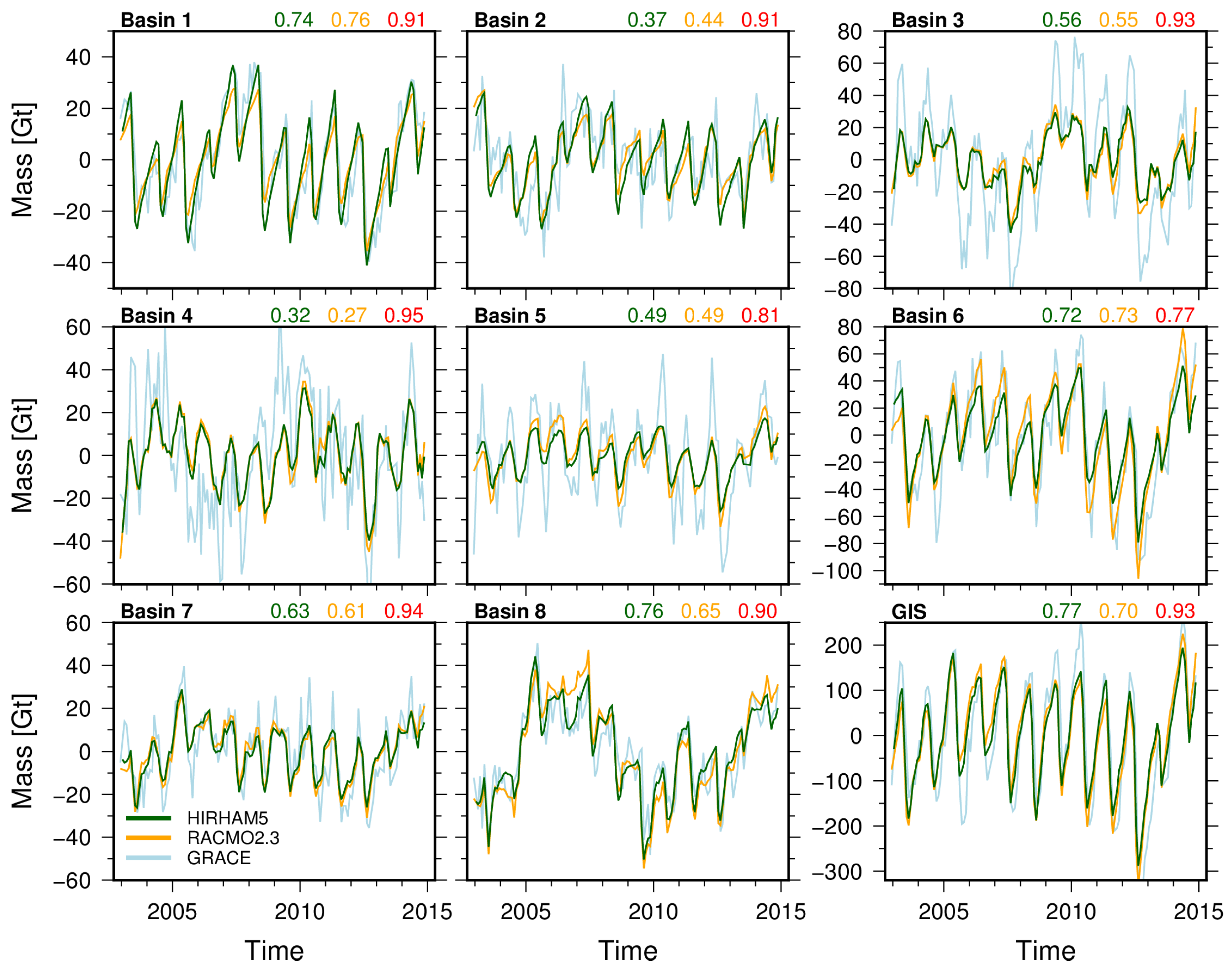
3.3. Total Ice Sheet Mass Budget down to the Basin Scale
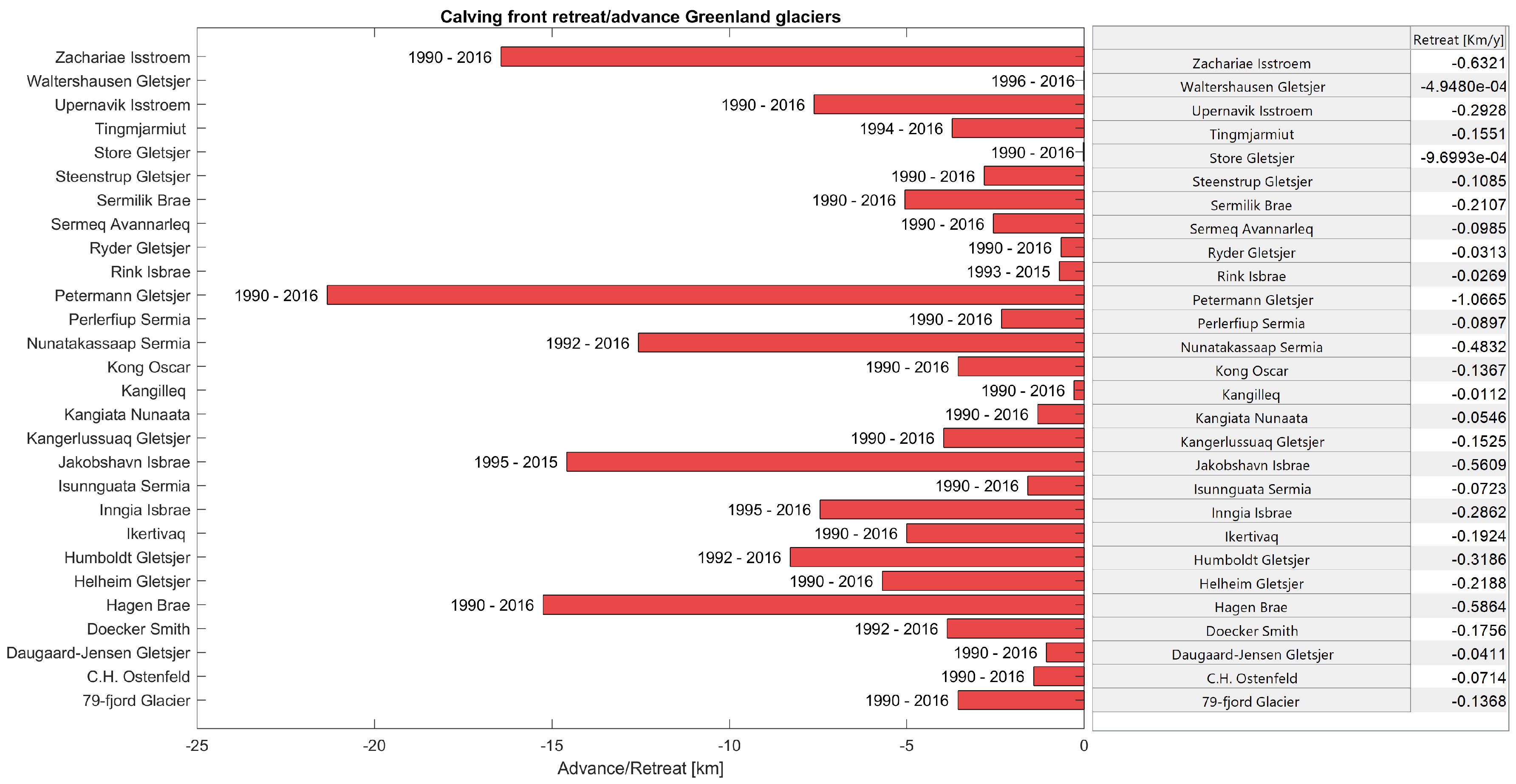
3.4. Calving Front Location and Ice Sheet Mass Budget
4. Outlook
5. Conclusions
Supplementary Materials
Author Contributions
Acknowledgments
Conflicts of Interest
References
- Van den Broeke, M.R.; Enderlin, E.M.; Howat, I.M.; Kuipers Munneke, P.; Noël, B.P.Y.; van de Berg, W.J.; van Meijgaard, E.; Wouters, B. On the recent contribution of the Greenland ice sheet to sea level change. Cryosphere 2016, 10, 1933–1946. [Google Scholar] [CrossRef] [Green Version]
- Shepherd, A.; Ivins, E.R.; Geruo, A.; Barletta, V.R.; Bentley, M.J.; Bettadpur, S.; Briggs, K.H.; Bromwich, D.H.; Forsberg, R.; Galin, N.; et al. A Reconciled Estimate of Ice-Sheet Mass Balance. Science 2012, 338, 1183–1189. [Google Scholar] [CrossRef] [PubMed] [Green Version]
- Vaughan, D.G.; Comiso, J.C.; Allison, I.; Carrasco, J.; Kaser, G.; Kwok, R.; Mote, P.; Murray, T.; Paul, F.; Ren, J.; et al. Observations: Cryosphere. Clim. Chang. 2013, 2103, 317–382. [Google Scholar]
- Cappelen, J. Greenland-Dmi Historical Climate Data Collection 1784-2017; Danish Meteorological Institue Report 18-04; Danish Meteorological Institute: Copenhagen, Denmark, 2017. [Google Scholar]
- Langen, P.L.; Fausto, R.S.; Vandecrux, B.; Mottram, R.H.; Box, J.E. Liquid Water Flow and Retention on the Greenland Ice Sheet in the Regional Climate Model HIRHAM5: Local and Large-Scale Impacts. Front. Earth Sci. 2017, 4. [Google Scholar] [CrossRef] [Green Version]
- Rignot, E.; Fenty, I.; Xu, Y.; Cai, C.; Kemp, C. Undercutting of marine-terminating glaciers in West Greenland. Geophys. Res. Lett. 2015, 42, 5909–5917. [Google Scholar] [CrossRef] [PubMed]
- Enderlin, E.M.; Howat, I.M.; Jeong, S.; Noh, M.J.; Angelen, J.H.; Broeke, M.R. An improved mass budget for the Greenland ice sheet. Geophys. Res. Lett. 2014, 41, 866–872. [Google Scholar] [CrossRef] [Green Version]
- Akperov, M.; Rinke, A.; Mokhov, I.I.; Matthes, H.; Semenov, V.A.; Adakudlu, M.; Cassano, J.; Christensen, J.H.; Dembitskaya, M.A.; Dethloff, K.; et al. Cyclone Activity in the Arctic From an Ensemble of Regional Climate Models (Arctic CORDEX). J. Geophys. Res. Atmos. 2018, 123, 2537–2554. [Google Scholar] [CrossRef]
- Lucas-Picher, P.; Wulff-Nielsen, M.; Christensen, J.H.; Aðalgeirsdóttir, G.; Mottram, R.; Simonsen, S.B. Very high resolution regional climate model simulations over Greenland: Identifying added value: RCM SIMULATIONS FOR GREENLAND. J. Geophys. Res. Atmos. 2012, 117. [Google Scholar] [CrossRef]
- Noel, B.; van de Berg, W.; van Meijgaard, E.; Kuipers Munneke, P.; van de Wal, R.; van den Broeke, M. Evaluation of the updated regional climate model RACMO2.3: summer snowfall impact on the Greenland Ice Sheet. Cryosphere 2015, 9, 1831–1844. [Google Scholar] [CrossRef] [Green Version]
- Van Tricht, K.; Lhermitte, S.; Lenaerts, J.T.M.; Gorodetskaya, I.V.; L’Ecuyer, T.S.; Noël, B.; van den Broeke, M.R.; Turner, D.D.; van Lipzig, N.P.M. Clouds enhance Greenland ice sheet meltwater runoff. Nat. Commun. 2016, 7, 10266. [Google Scholar] [CrossRef]
- Mottram, R.; Nielsen, K.P.; Gleeson, E.; Yang, X. Modelling Glaciers in the HARMONIE-AROME NWP model. Adv. Sci. Res. 2017, 14, 323–334. [Google Scholar] [CrossRef] [Green Version]
- Vernon, C.L.; Bamber, J.L.; Box, J.E.; van den Broeke, M.R.; Fettweis, X.; Hanna, E.; Huybrechts, P. Surface mass balance model intercomparison for the Greenland ice sheet. Cryosphere 2013, 7, 599–614. [Google Scholar] [CrossRef] [Green Version]
- Adalgeirsdottir, G.; Aschwanden, A.; Khroulev, C.; Boberg, F.; Mottram, R.; Lucas-Picher, P.; Christensen, J.H. Role of model initialization for projections of 21st-century Greenland ice sheet mass loss. J. Glaciol. 2014, 60, 782–794. [Google Scholar] [CrossRef] [Green Version]
- Joughin, I.; Fahnestock, M.; Kwok, R.; Gogineni, P.; Allen, C. Ice flow of Humboldt, Petermann and Ryder Gletscher, northern Greenland. J. Glaciol. 1999, 45, 231–241. [Google Scholar] [CrossRef] [Green Version]
- Hogg, A.E.; Shepherd, A.; Gourmelen, N.; Engdahl, M. Grounding line migration from 1992 to 2011 on Petermann Glacier, North-West Greenland. J. Glaciol. 2016, 62, 1104–1114. [Google Scholar] [CrossRef] [Green Version]
- Sørensen, L.S.; Simonsen, S.B.; Nielsen, K.; Lucas-Picher, P.; Spada, G.; Adalgeirsdottir, G.; Forsberg, R.; Hvidberg, C.S. Mass balance of the Greenland ice sheet (2003–2008) from ICESat data—The impact of interpolation, sampling and firn density. Cryosphere 2011, 5, 173–186. [Google Scholar] [CrossRef]
- Sørensen, L.S.; Simonsen, S.B.; Meister, R.; Forsberg, R.; Levinsen, J.F.; Flament, T. Envisat-derived elevation changes of the Greenland ice sheet, and a comparison with ICESat results in the accumulation area. Remote Sens. Environ. 2015, 160, 56–62. [Google Scholar] [CrossRef]
- Simonsen, S.B.; Sørensen, L.S. Implications of changing scattering properties on Greenland ice sheet volume change from Cryosat-2 altimetry. Remote Sens. Environ. 2017, 190, 207–216. [Google Scholar] [CrossRef]
- Sandberg Sørensen, L.; Simonsen, S.B.; Forsberg, R.; Khvorostovsky, K.; Meister, R.; Engdahl, M.E. 25 years of elevation changes of the Greenland Ice Sheet from ERS, Envisat, and CryoSat-2 radar altimetry. Earth Planet. Sci. Lett. 2018, 495, 234–241. [Google Scholar] [CrossRef]
- Rathmann, N.M.; Hvidberg, C.S.; Solgaard, A.M.; Grinsted, A.; Gudmundsson, G.H.; Langen, P.L.; Nielsen, K.P.; Kusk, A. Highly temporally resolved response to seasonal surface melt of the Zachariae and 79N outlet glaciers in northeast Greenland. Geophys. Res. Lett. 2017, 44, 9805–9814. [Google Scholar] [CrossRef] [Green Version]
- Nagler, T.; Rott, H.; Hetzenecker, M.; Wuite, J.; Potin, P. The Sentinel-1 Mission: New Opportunities for Ice Sheet Observations. Remote Sens. 2015, 7, 9371–9389. [Google Scholar] [CrossRef] [Green Version]
- Simonsen, S.B.; Stenseng, L.; Ađalgeirsdóttir, G.; Fausto, R.S.; Hvidberg, C.S.; Lucas-Picher, P. Assessing a multilayered dynamic firn-compaction model for Greenland with ASIRAS radar measurements. J. Glaciol. 2013, 59, 545–558. [Google Scholar] [CrossRef]
- Boncori, J.P.M.; Andersen, M.L.; Dall, J.; Kusk, A.; Kamstra, M.; Andersen, S.B.; Bechor, N.; Bevan, S.; Bignami, C.; Gourmelen, N.; et al. Intercomparison and Validation of SAR-Based Ice Velocity Measurement Techniques within the Greenland Ice Sheet CCI Project. Remote Sens. 2018, 10, 929. [Google Scholar] [CrossRef]
- Joughin, I. MEaSUREs Greenland Ice Sheet Velocity Map from InSAR Data, Version 2; National Snow and Ice Data Center: Boulder, CO, USA, 2015. [Google Scholar]
- Khvorostovsky, K. Algorithm Theoretical Baseline Document (ATBD) for the Greenland Ice Sheet CCI Project of ESA’s Climate Change Initiative, Version 3.2. Available online: http://esa-icesheets-greenland-cci.org/sites/default/files/documents/public/Phase (accessed on 30 May 2019).
- Benn, D.I.; Warren, C.R.; Mottram, R.H. Calving processes and the dynamics of calving glaciers. Earth-Sci. Rev. 2007, 82, 143–179. [Google Scholar] [CrossRef]
- Schoof, C. Ice sheet grounding line dynamics: Steady states, stability, and hysteresis. J. Geophys. Res. Earth Surf. 2007, 112. [Google Scholar] [CrossRef] [Green Version]
- Mouginot, J.; Rignot, E.; Scheuchl, B.; Fenty, I.; Khazendar, A.; Morlighem, M.; Buzzi, A.; Paden, J. Fast retreat of Zachariæ Isstrøm, northeast Greenland. Science 2015, 350, 1357–1361. [Google Scholar] [CrossRef] [PubMed]
- Rignot, E.; Velicogna, I.; van den Broeke, M.R.; Monaghan, A.; Lenaerts, J.T. Acceleration of the contribution of the Greenland and Antarctic ice sheets to sea level rise. Geophys. Res. Lett. 2011, 38. [Google Scholar] [CrossRef] [Green Version]
- Rignot, E.; Mouginot, J.; Scheuchl, B. Antarctic grounding line mapping from differential satellite radar interferometry: GROUNDING LINE OF ANTARCTICA. Geophys. Res. Lett. 2011, 38. [Google Scholar] [CrossRef]
- Nagler, T. Comprehensive Error Characterisation Report (CECR). Antarctic Ice Sheet cci project, ESA’s Climate Change Initiative, Version 3.0. 2018. Available online: http://esa-icesheets-antarctica-cci.org/index.php?q=webfm_send/84 (accessed on 30 May 2019).
- Davis, C.; Ferguson, A. Elevation change of the Antarctic ice sheet, 1995–2000, from ERS-2 satellite radar altimetry. IEEE Trans. Geosci. Remote Sens. 2004, 42, 2437–2445. [Google Scholar] [CrossRef]
- Johannessen, O.M. Recent Ice-Sheet Growth in the Interior of Greenland. Science 2005, 310, 1013–1016. [Google Scholar] [CrossRef] [Green Version]
- Khvorostovsky, K.S. Merging and Analysis of Elevation Time Series Over Greenland Ice Sheet From Satellite Radar Altimetry. IEEE Trans. Geosci. Remote Sens. 2012, 50, 23–36. [Google Scholar] [CrossRef]
- Levinsen, J.; Khvorostovsky, K.; Ticconi, F.; Shepherd, A.; Forsberg, R.; Sørensen, L.; Muir, A.; Pie, N.; Felikson, D.; Flament, T.; et al. ESA ice sheet CCI: derivation of the optimal method for surface elevation change detection of the Greenland ice sheet—Round robin results. Int. J. Remote Sens. 2015, 36, 551–573. [Google Scholar] [CrossRef]
- Tapley, B.; Bettadpur, S.; Watkins, M.; Reigber, C. The gravity recovery and climate experiment: Mission overview and early results. Geophys. Res. Lett. 2004, 31, L09607. [Google Scholar] [CrossRef]
- Mayer-Gürr, T.; Behzadpour, S.; Ellmer, M.; Kvas, A.; Klinger, B.; Zehentner, N. ITSG-Grace2016–Monthly and Daily Gravity Field Solutions from GRACE. GFZ Data Serv. 2016. [Google Scholar] [CrossRef]
- Bettadpur, S. UTCSR Level-2 Processing Standards Document for Level-2 Product Release 0006; Technical Report; University of Texas at Austin: Austin, TX, USA, 2018. [Google Scholar]
- Zwally, H.; Giovinetto, M.; Beckley, M.; Saba, J. Antarctic and Greenland Drainage Systems. Available online: http://icesat4.gsfc.nasa.gov/cryo_data/ant_grn_drainage_systems.php (accessed on 30 May 2019).
- Barletta, V.R.; Sørensen, L.S.; Forsberg, R. Scatter of mass changes estimates at basin scale for Greenland and Antarctica. Cryosphere 2013, 7, 1411–1432. [Google Scholar] [CrossRef] [Green Version]
- Groh, A.; Horwath, M. The method of tailored sensitivity kernels for GRACE mass change estimates. In Proceedings of the EGU General Assembly 2016, Vienna, Austria, 17–22 April 2016; Volume 18. [Google Scholar]
- Wahr, J.; Zhong, S. Computations of the viscoelastic response of a 3-D compressible Earth to surface loading: An application to Glacial Isostatic Adjustment in Antarctica and Canada. Geophys. J. Int. 2013, 192, 557–572. [Google Scholar] [CrossRef]
- Peltier, W.; Argus, D.; Drummond, R. Space geodesy constrains ice age terminal deglaciation: The global ICE-6G_C (VM5a) model: Global Glacial Isostatic Adjustment. J. Geophys. Res. Solid Earth 2015, 120, 450–487. [Google Scholar] [CrossRef]
- Mottram, R.; Boberg, F.; Langen, P.; Yang, S.; Rodehacke, C.; Christensen, J.H.; Madsen, M.S. Surface Mass balance of the Greenland ice Sheet in the Regional Climate Model HIRHAM5: Present State and Future Prospects. Low Temp. Sci. 2017, 75, 1–11. [Google Scholar] [CrossRef]
- Sasgen, I.; van den Broeke, M.; Bamber, J.; Rignot, E.; Sørensen, L.; Wouters, B.; Martinec, Z.; Velicogna, I.; Simonsen, S. Timing and origin of recent regional ice-mass loss in Greenland. Earth Planet. Sci. Lett. 2012, 333–334, 293–303. [Google Scholar] [CrossRef]
- Van den Broeke, M.; Bamber, J.; Ettema, J.; Rignot, E.; Schrama, E.; van de Berg, W.J.; van Meijgaard, E.; Velicogna, I.; Wouters, B. Partitioning Recent Greenland Mass Loss. Science 2009, 326, 984–986. [Google Scholar] [CrossRef] [Green Version]
- Dee, D.P.; Uppala, S.M.; Simmons, A.; Berrisford, P.; Poli, P.; Kobayashi, S.; Andrae, U.; Balmaseda, M.; Balsamo, G.; Bauer, D.P.; et al. The ERA-Interim reanalysis: Configuration and performance of the data assimilation system. Q. J. R. Meteorol. Soc. 2011, 137, 553–597. [Google Scholar] [CrossRef]
- Roeckner, E.; Oberhuber, J.M.; Bacher, A.; Christoph, M.; Kirchner, I. ENSO variability and atmospheric response in a global coupled atmosphere-ocean GCM. Clim. Dyn. 1996, 12, 737–754. [Google Scholar] [CrossRef] [Green Version]
- Rae, J.G.L.; Aðalgeirsdóttir, G.; Edwards, T.L.; Fettweis, X.; Gregory, J.M.; Hewitt, H.T.; Lowe, J.A.; Lucas-Picher, P.; Mottram, R.H.; Payne, A.J.; et al. Greenland ice sheet surface mass balance: Evaluating simulations and making projections with regional climate models. Cryosphere 2012, 6, 1275–1294. [Google Scholar] [CrossRef]
- Langen, P.L.; Mottram, R.H.; Christensen, J.H.; Boberg, F.; Rodehacke, C.B.; Stendel, M.; van As, D.; Ahlstrøm, A.P.; Mortensen, J.; Rysgaard, S.; et al. Quantifying Energy and Mass Fluxes Controlling Godthåbsfjord Freshwater Input in a 5-km Simulation (1991–2012). J. Clim. 2015, 28, 3694–3713. [Google Scholar] [CrossRef]
- Eerola, K. Twenty-one years of verification from the HIRLAM NWP system. Weather Forecast. 2013, 28, 270–285. [Google Scholar] [CrossRef]
- Hermann, M.; Box, J.E.; Fausto, R.S.; Colgan, W.T.; Langen, P.L.; Mottram, R.; Wuite, J.; Noël, B.; van den Broeke, M.R.; van As, D. Application of PROMICE Q-Transect in Situ Accumulation and Ablation Measurements (2000–2017) to Constrain Mass Balance at the Southern Tip of the Greenland Ice Sheet. J. Geophys. Res. Earth Surf. 2018, 123, 1235–1256. [Google Scholar] [CrossRef]
- Mote, T.L.; Anderson, M.R. Variations in snowpack melt on the Greenland ice sheet based on passive-microwave measurements. J. Glaciol. 1995, 41, 51–60. [Google Scholar] [CrossRef] [Green Version]
- Ettema, J.; van den Broeke, M.R.; van Meijgaard, E.; van de Berg, W.J.; Bamber, J.L.; Box, J.E.; Bales, R.C. Higher surface mass balance of the Greenland ice sheet revealed by high-resolution climate modeling. Geophys. Res. Lett. 2009, 36. [Google Scholar] [CrossRef] [Green Version]
- Fettweis, X.; Franco, B.; Tedesco, M.; van Angelen, J.H.; Lenaerts, J.T.M.; van den Broeke, M.R.; Gallae, H. Estimating the Greenland ice sheet surface mass balance contribution to future sea level rise using the regional atmospheric climate model MAR. Cryosphere 2013, 7, 469–489. [Google Scholar] [CrossRef] [Green Version]
- Vizcaino, M. Ice sheets as interactive components of Earth System Models: Progress and challenges. WIRES Clim. Chang. 2014, 5, 557–568. [Google Scholar] [CrossRef]
- Goelzer, H.; Robinson, A.; Seroussi, H.; van de Wal, R.S. Recent Progress in Greenland Ice Sheet Modelling. Curr. Clim. Chang. Rep. 2017, 3, 291–302. [Google Scholar] [CrossRef] [Green Version]
- Kirchner, N.; Hutter, K.; Jakobsson, M.; Gyllencreutz, R. Capabilities and limitations of numerical ice sheet models; a discussion for Earth-scientists and modelers. Q. Sci. Rev. 2011, 30, 3691–3704. [Google Scholar] [CrossRef]
- Bueler, E.; Brown, J.; Lingle, C. Exact solutions to the thermomechanically coupled shallow ice approximation: effective tools for verification. J. Glaciol. 2007, 53, 499–516. [Google Scholar] [CrossRef]
- Aschwanden, A.; Bueler, E.; Khroulev, C.; Blatter, H. An enthalpy formulation for glaciers and ice sheets. J. Glaciol. 2012, 58, 441–457. [Google Scholar] [CrossRef] [Green Version]
- Theoretical Glaciology: Mateial Science of Ice and the Mechanics of Glaciers and Ice Sheets; Number 1 in Mathematical Approaches to Geophysics; Springer: Berlin/Heidelberg, Germany, 1983.
- Morland, L. Plane and Radial Ice-Shelf Flow with Prescirpbed Temperature Profile. In Dynamics of the West Antarctic Ice Sheet; van der Veen, C.J., Oelemans, J., Eds.; D. Reidel Publishing Company: Dordrecht, The Netherlands, 1987. [Google Scholar]
- Bueler, E.; Brown, J. Shallow shelf approximation as a “sliding law” in a thermomechanically coupled ice sheet model. J. Geophys. Res. Earth Surf. 2009, 114. [Google Scholar] [CrossRef]
- Aschwanden, A.; Fahnestock, M.A.; Truffer, M. Complex Greenland outlet glacier flow captured. Nat. Commun. 2016, 7, 10524. [Google Scholar] [CrossRef]
- Khroulev, C.; PISM Authors. PISM, a Parallel Ice Sheet Model: User’s Manual. Available online: http://pism-docs.org/wiki/lib/exe/fetch.php?media=pism_manual.pdf (accessed on 31 May 2019).
- Bamber, J.; Layberry, R.; Gogenini, S. A new ice thickness and bed data set for the Greenland ice sheet1: Measurement, data reduction, and errors. J. Geophys. Res. 2001, 106, 33773–33780. [Google Scholar] [CrossRef]
- Nowicki, S.; Bindschadler, R.A.; Abe-Ouchi, A.; Aschwanden, A.; Bueler, E.; Choi, H.; Fastook, J.; Granzow, G.; Greve, R.; Gutowski, G.; et al. Insight into spatial sensitivities of ice mass response to environmental change from the SeaRISE ice sheet modeling project II: Greenland. J. Geophys. Res. 2013, 118, 1025–1044. [Google Scholar] [CrossRef]
- Velicogna, I.; Wahr, J. Acceleration of Greenland ice mass loss in spring 2004. Nature 2006, 443, 329–331. [Google Scholar] [CrossRef] [Green Version]
- Svendsen, P.; Andersen, O.; Nielsen, A. Acceleration of the Greenland ice sheet mass loss as observed by GRACE: Confidence and sensitivity. Earth Planet. Sci. Lett. 2013, 364, 24–29. [Google Scholar] [CrossRef]
- Krabill, W.; Hanna, E.; Huybrechts, P.; Abdalati, W.; Cappelen, J.; Csatho, B.; Frederick, E.; Manizade, S.; Martin, C.; Sonntag, J.; et al. Greenland Ice Sheet: Increased coastal thinning. Geophys. Res. Lett. 2004, 31. [Google Scholar] [CrossRef] [Green Version]
- Colgan, W.; Rajaram, H.; Abdalati, W.; McCutchan, C.; Mottram, R.; Moussavi, M.S.; Grigsby, S. Glacier crevasses: Observations, models, and mass balance implications: Glacier Crevasses. Rev. Geophys. 2016, 54, 119–161. [Google Scholar] [CrossRef]
- Nick, F.; Van Der Veen, C.; Vieli, A.; Benn, D. A physically based calving model applied to marine outlet glaciers and implications for the glacier dynamics. J. Glaciol. 2010, 56, 781–794. [Google Scholar] [CrossRef] [Green Version]
- Porter, D.F.; Tinto, K.J.; Boghosian, A.L.; Csatho, B.M.; Bell, R.E.; Cochran, J.R. Identifying Spatial Variability in Greenland’s Outlet Glacier Response to Ocean Heat. Front. Earth Sci. 2018, 6, 90. [Google Scholar] [CrossRef]
- Fahnestock, M.; Abdalati, W.; Joughin, I.; Brozena, J.; Gogineni, P. High Geothermal Heat Flow, Basal Melt, and the Origin of Rapid Ice Flow in Central Greenland. Science 2001, 294, 2338–2342. [Google Scholar] [CrossRef] [Green Version]
- Christanson, K.; Peters, L.E.; Alley, R.B.; Anandakrishnan, S.; Jacobel, R.W.; Riverman, K.L.; Muto, A.; Keisling, B.A. Dilatant till facilitates ice-stream flow in northeast Greenland. Earth Planet. Sci. Lett. 2014, 401, 57–69. [Google Scholar] [CrossRef]
- Rogozhina, I.; Petrunin, A.G.; Vaughan, A.P.; Steinberger, B.; Johnson, J.V.; Kaban, M.K.; Reinhard, C.; Rickers, F.; Thomas, M.; Koulakov, I. Melting at the base of the Greenland ice sheet explained by Iceland hotspot history. Nat. Geosci. 2016, 9, 366–369. [Google Scholar] [CrossRef] [Green Version]
- Wahr, J.; Swenson, S.; Velicogna, I. Accuracy of GRACE mass estimates. Geophys. Res. Lett. 2006, 33. [Google Scholar] [CrossRef] [Green Version]
- Moon, T.; Joughin, I.; Smith, B. Seasonal to multiyear variability of glacier surface velocity, terminus position, and sea ice/ice mélange in northwest Greenland. J. Geophys. Res. Earth Surf. 2015, 120, 818–833. [Google Scholar] [CrossRef]
- Tedesco, M.; Doherty, S.; Fettweis, X.; Alexander, P.; Jeyaratnam, J.; Stroeve, J. The darkening of the Greenland ice sheet: trends, drivers, and projections (1981–2100). Cryosphere 2016, 10, 477–496. [Google Scholar] [CrossRef]
- Fausto, R.; van As, D.; Box, J.; Colgan, W.; Langen, P. Quantifying the surface energy fluxes in South Greenland during the 2012 high melt episodes using in-situ observations. Front. Earth Sci. 2016, 4, 82. [Google Scholar] [CrossRef]
- Smith, L.C.; Yang, K.; Pitcher, L.H.; Overstreet, B.T.; Chu, V.W.; Rennermalm, A.K.; Ryan, J.C.; Cooper, M.G.; Gleason, C.J.; Tedesco, M.; et al. Direct measurements of meltwater runoff on the Greenland ice sheet surface. Proc. Natl. Acad. Sci. USA 2017, 114, E10622–E10631. [Google Scholar] [CrossRef] [PubMed] [Green Version]
- Benn, D.I.; Cowton, T.; Todd, J.; Luckman, A. Glacier Calving in Greenland. Curr. Clim. Chang. Rep. 2017, 3, 282–290. [Google Scholar] [CrossRef] [Green Version]
- Goelzer, H.; Nowicki, S.; Edwards, T.; Beckley, M.; Abe-Ouchi, A.; Aschwanden, A.; Calov, R.; Gagliardini, O.; Gillet-Chaulet, F.; Golledge, N.R.; et al. Design and results of the ice sheet model initialisation experiments initMIP-Greenland: An ISMIP6 intercomparison. Cryosphere 2018, 12, 1433–1460. [Google Scholar] [CrossRef]
- Hill, E.A.; Carr, J.R.; Stokes, C.R.; Gudmundsson, G.H. Dynamic changes in outlet glaciers in northern Greenland from 1948 to 2015. Cryosphere 2018, 12, 3243–3263. [Google Scholar] [CrossRef] [Green Version]
- Nick, F.; Luckman, A.; Vieli, A.; Van Der Veen, C.; Van As, D.; Van De Wal, R.; Pattyn, F.; Hubbard, A.; Floricioiu, D. The response of Petermann Glacier, Greenland, to large calving events, and its future stability in the context of atmospheric and oceanic warming. J. Glaciol. 2012, 58, 229–239. [Google Scholar] [CrossRef] [Green Version]
- Morlighem, M.; Williams, C.N.; Rignot, E.; An, L.; Arndt, J.E.; Bamber, J.L.; Catania, G.; Chauché, N.; Dowdeswell, J.A.; Dorschel, B.; et al. BedMachine v3: Complete Bed Topography and Ocean Bathymetry Mapping of Greenland From Multibeam Echo Sounding Combined With Mass Conservation. Geophys. Res. Lett. 2017, 4, 11051–11061. [Google Scholar] [CrossRef]
- Rückamp, M.; Neckel, N.; Berger, S.; Humbert, A.; Helm, V. Calving Induced Speedup of Petermann Glacier. J. Geophys. Res. Earth Surf. 2019. [Google Scholar] [CrossRef]
- Rosier, J.; Mottram, R.; Lhermitte, S.; Hetzenecker, M. Channelised melting and fracturing provide early warning of petermann ice shelf collapse. Sci. Adv. 2019. under review. [Google Scholar]
- Mottram, R.H.; Benn, D.I. Testing crevasse-depth models: A field study at Breidamerkurjokull, Iceland. J. Glaciol. 2009, 55, 746–752. [Google Scholar] [CrossRef]
- Glen, J.W. The Creep of Polycrystalline Ice. Proc. R. Soc. A Math. Phys. Eng. Sci. 1955, 228, 519–538. [Google Scholar] [CrossRef]
- Van der Veen, C. Fracture mechanics approach to penetration of surface crevasses on glaciers. Cold Regions Sci. Technol. 1998, 27, 31–47. [Google Scholar] [CrossRef]
- MacDonald, G.; Banwell, A.; MacAyeal, D.R. Seasonal evolution of supraglacial lakes on a floating ice tongue, Petermann Glacier, Greenland. Ann. Glaciol. 2018, 1–10. [Google Scholar] [CrossRef]
- Dow, C.F.; Lee, W.S.; Greenbaum, J.S.; Greene, C.A.; Blankenship, D.D.; Poinar, K.; Forrest, A.L.; Young, D.A.; Zappa, C.J. Basal channels drive active surface hydrology and transverse ice shelf fracture. Sci. Adv. 2018, 4, eaao7212. [Google Scholar] [CrossRef] [PubMed] [Green Version]
- Rignot, E.; Steffen, K. Channelized bottom melting and stability of floating ice shelves. Geophys. Res. Lett. 2008, 35. [Google Scholar] [CrossRef] [Green Version]
- Bengtsson, L.; Andrae, U.; Aspelien, T.; Batrak, Y.; Calvo, J.; de Rooy, W.; Gleeson, E.; Hansen-Sass, B.; Homleid, M.; Hortal, M.; et al. The HARMONIE—AROME Model Configuration in the ALADIN–HIRLAM NWP System. Mon. Weather Rev. 2017, 145, 1919–1935. [Google Scholar] [CrossRef]
- Münchow, A.; Padman, L.; Fricker, H.A. Interannual changes of the floating ice shelf of Petermann Gletscher, North Greenland, from 2000 to 2012. J. Glaciol. 2014, 60, 489–499. [Google Scholar] [CrossRef] [Green Version]


© 2019 by the authors. Licensee MDPI, Basel, Switzerland. This article is an open access article distributed under the terms and conditions of the Creative Commons Attribution (CC BY) license (http://creativecommons.org/licenses/by/4.0/).
Share and Cite
Mottram, R.; B. Simonsen, S.; Høyer Svendsen, S.; Barletta, V.R.; Sandberg Sørensen, L.; Nagler, T.; Wuite, J.; Groh, A.; Horwath, M.; Rosier, J.; et al. An Integrated View of Greenland Ice Sheet Mass Changes Based on Models and Satellite Observations. Remote Sens. 2019, 11, 1407. https://0-doi-org.brum.beds.ac.uk/10.3390/rs11121407
Mottram R, B. Simonsen S, Høyer Svendsen S, Barletta VR, Sandberg Sørensen L, Nagler T, Wuite J, Groh A, Horwath M, Rosier J, et al. An Integrated View of Greenland Ice Sheet Mass Changes Based on Models and Satellite Observations. Remote Sensing. 2019; 11(12):1407. https://0-doi-org.brum.beds.ac.uk/10.3390/rs11121407
Chicago/Turabian StyleMottram, Ruth, Sebastian B. Simonsen, Synne Høyer Svendsen, Valentina R. Barletta, Louise Sandberg Sørensen, Thomas Nagler, Jan Wuite, Andreas Groh, Martin Horwath, Job Rosier, and et al. 2019. "An Integrated View of Greenland Ice Sheet Mass Changes Based on Models and Satellite Observations" Remote Sensing 11, no. 12: 1407. https://0-doi-org.brum.beds.ac.uk/10.3390/rs11121407