Convolutional Neural Networks for On-Board Cloud Screening


Electronics and Telecommunication Department, Polytechnic University of Turin, 10129 Turin, Italy
*
Author to whom correspondence should be addressed.
Remote Sens. 2019, 11(12), 1417; https://0-doi-org.brum.beds.ac.uk/10.3390/rs11121417
Submission received: 8 May 2019
/
Revised: 10 June 2019
/
Accepted: 12 June 2019
/
Published: 14 June 2019
(This article belongs to the Special Issue Real-Time Processing of Remotely-Sensed Imaging Data)
Abstract
:A cloud screening unit on a satellite platform for Earth observation can play an important role in optimizing communication resources by selecting images with interesting content while skipping those that are highly contaminated by clouds. In this study, we address the cloud screening problem by investigating an encoder–decoder convolutional neural network (CNN). CNNs usually employ millions of parameters to provide high accuracy; on the other hand, the satellite platform imposes hardware constraints on the processing unit. Hence, to allow an onboard implementation, we investigate experimentally several solutions to reduce the resource consumption by CNN while preserving its classification accuracy. We experimentally explore approaches such as halving the computation precision, using fewer spectral bands, reducing the input size, decreasing the number of network filters and also making use of shallower networks, with the constraint that the resulting CNN must have sufficiently small memory footprint to fit the memory of a low-power accelerator for embedded systems. The trade-off between the network performance and resource consumption has been studied over the publicly available SPARCS dataset. Finally, we show that the proposed network can be implemented on the satellite board while performing with reasonably high accuracy compared with the state-of-the-art.
1. Introduction
In recent years, the rapid advance of remote sensing technology has allowed acquiring high-resolution images over a large geographical scale which can be employed in a broad range of applications such as environmental monitoring, agriculture, land-use analysis and so on. Nevertheless, clouds are estimated to cover about 66% of the Earth surface [1], potentially contaminating a large portion of the captured images. Such contamination masks objects on the Earth surface making the affected images useless for analysis. Therefore, onboard cloud screening can in principle be applied on the satellite platform as a pre-processing step before image compression and transmission, selecting images with a low cloud cover percentage and discarding the others, thereby avoiding processing and transmitting the images which are covered by clouds.
A very well-known cloud detection algorithm is F1-mask [2], which is employed on Landsat imagery and employs top-of-atmosphere reflectance and brightness temperature for all Landsat bands, detecting cloudy pixels through a series of spectral tests. Similarly, authors in [3] report that the EO-1 spacecraft employs calculation of top-of-atmosphere reflectance followed by a few threshold tests in order to perform onboard cloud screening. While this is the first demonstration of cloud screening, screening a 1024 × 256 image requires about 30 min, which is far too much for real-time processing. In addition, as many traditional remote sensing approaches make use of handcrafted features such as pixel shape index [4] or morphological functions [5,6,7,8], such features are also found to be an effective tool to detect clouds as described by authors in [9] over images acquired by SPOT Earth observation satellites. More recently, cloud detection has been addressed by employing machine learning techniques including Bayesian statistical techniques [10,11], decision-tree classifier [12], support vector machine [13] and also random forest [14]. Finally, authors in [15] study a combination of machine learning approaches such as linear, quadratic and nonparametric discriminant analysis, principal component and independent component discriminant analysis to handle the cloud detection over MODIS images.
The recent decade has witnessed rapid development in the area of deep learning leading to outstanding performance in many fields including computer vision. Well-known convolutional neural networks (CNNs) have advanced the state-of-the-art in many computer vision tasks such as image classification and semantic segmentation [16,17,18,19,20,21]. Not an exception to such trend, remote sensing has been also enjoying the benefits of deep learning algorithms in achieving state-of-the-art performance in many tasks such as land-use classification and segmentation [22,23,24,25,26,27]. CNNs usually consist of thousands of filters with millions of learnable parameters which are trained to detect semantic representations useful for a particular task and over a large amount of annotated images. Regarding cloud detection, recent studies have been carried out to make use of CNNs also in performing such detection task [28,29,30,31]. For instance, in [28], to perform cloud detection, satellite images first undergo a simple linear iterative clustering process in which homogeneous pixels are clustered into superpixels; then, a four-layer CNN is employed to extract features and, finally, two fully connected layers predict the superpixels class. In [29], authors show that a similar CNN architecture with six convolutional layers operating on 32 × 32 patches when combined with superpixel clustering can perform cloud detection with reasonably high accuracy on SPOT 6 images. A very well-known CNN architecture that is widely used in many segmentation tasks is U-net. U-net is originally proposed to address biomedical image segmentation [32] and it employs a simple yet effective architecture consisting of an encoder and a decoder network which are connected through a number of skip connections. The use of skip connections contributes to finer segmentation results alleviating the need of post-processing steps, as the early spatial information of encoders is concatenated with feature maps in decoders providing higher resolution feature maps in the process of generating segmentation outputs. Authors in [33] address cloud detection over Landsat 8 images proposing an architecture similar to U-net. To train such network, first, a snow/ice removal framework that is based on gradient-based identification is applied over Quality Assessment (QA) band of Landsat images, then this layer is used as ground truth in the course of training. A lightweight convolutional encoder–decoder network is proposed in [31] to address cloud screening, whose input features are not the pixel values, but their wavelet coefficients. Authors construct experiments over the SPARCS (Spatial Procedures for Automated Removal of Cloud and Shadow) dataset [34,35] using 4 out of 11 bands and the proposed architecture outperforms common machine learning techniques such as AdaBoost, random forest and SVM by a considerable margin. The same architecture is used in [36] for high-resolution videos.
Cloud screening differs from cloud detection in that the outcome of the detection process is not used for scientific applications, but just to decide whether an image or part thereof has to be discarded. However, satellite board imposes hardware constraints on the cloud screening unit in terms of memory and power consumption. Additionally, in order to be useful, a cloud screening algorithm should be able to process an image in a near real-time manner with high precision.
In this study, we consider the cloud screening problem as a binary pixel-based segmentation problem where the image pixels are divided into cloud and non-cloud classes. We focus on multispectral images as such images do not contain finely-grained spectral information about the wavelengths at which clouds can be detected. Conversely, in hyperspectral images, one can pick a few wavelengths and efficiently detect the presence of clouds using very simple methods—see, e.g., [11].
To tackle such a problem, we also employ an encoder–decoder CNN inspired by U-net in which the encoder extracts visual representations (i.e., feature maps) over the input image, then the decoder takes as input such representations and generates segmentation maps. However, unlike previous work and original U-net architecture, we take into account the hardware limitations imposed by satellite platforms, by designing and testing several variants of this encoder–decoder network having different representation power, classification accuracy, memory footprint, and complexity. Since most state-of-the-art CNNs include millions of parameters, such limitations introduce unique challenges which require being addressed carefully. In particular, we study the trade-off between the resource consumption and the network performance in terms of classification accuracy by investigating several approaches such as limiting the number of network filters, decreasing the network depth, reducing the input size both in spatial and spectral domains and also operating on half-precision floating points. We provide our experimental results over the SPARCS publicly available dataset, and we show that the proposed network can perform close to the state-of-the-art CNNs, while consuming much fewer resources. In terms of resources, we consider that a low-power accelerator for embedded systems such as the Intel Myriad family typically provides 500 MB of memory to accommodate the neural network and input data, so we target the design of neural networks whose memory footprint is around this value or lower.
This paper is organized as follows. First, we describe the proposed methodology including the proposed network architecture, the sample generation procedure, and training process in Section 2; then, the experimental results over the SPARCS dataset are provided in Section 3 and finally we draw our conclusions in Section 4.
2. Methodology
In this section, first, we detail the architecture of the proposed network which we use as a baseline in our experiments. Then, the procedure used to generate training samples is described in detail. Next, the cost function used to optimize the network parameters and the related training process are defined.
2.1. Network Architecture
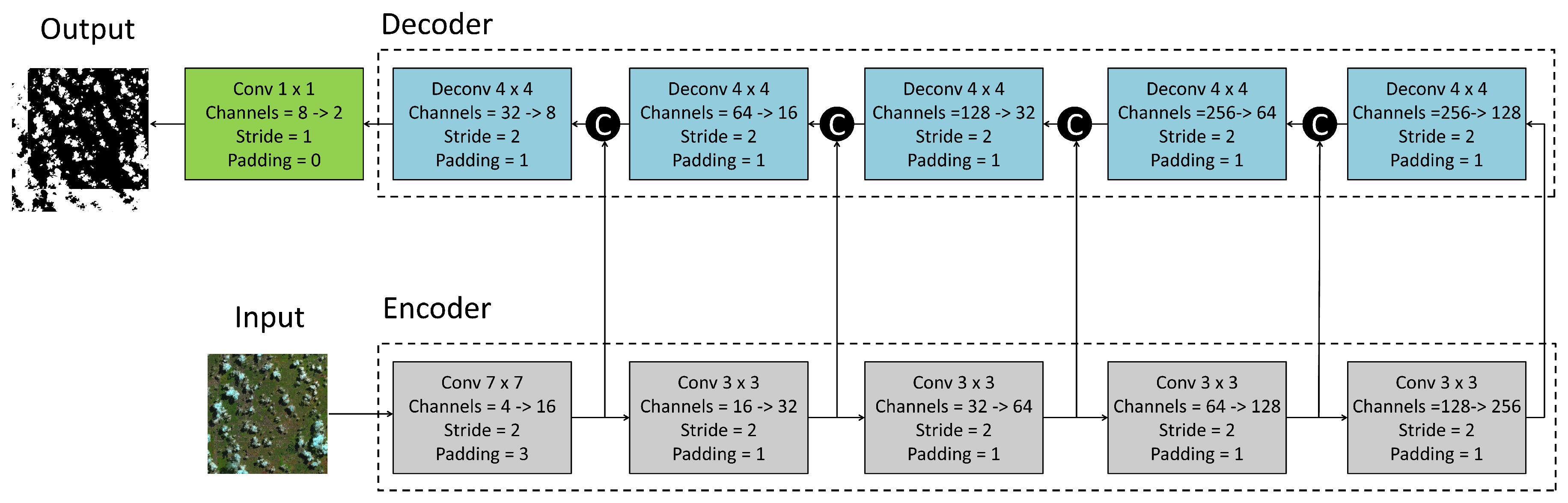
The proposed network as depicted in Figure 1 includes encoder and decoder networks. The encoder utilizes a sequence of convolutional layers to extract feature maps which can be seen as semantic representations of the input image. Then, the decoder takes as input such feature maps and, through deconvolutional layers, it generates the segmentation map which labels the pixels into cloud and non-cloud classes. In the following, we describe separately the architecture of encoder and decoder networks in detail.
2.1.1. Encoder
The encoder network includes five convolutional layers illustrated as gray blocks in Figure 1. Each convolutional layer is followed by a batch normalization layer and employs a rectified linear unit (ReLU) as activation function, except for the last convolutional layer before the output which employs sigmoid activations and performs the final classification as explained in the following section. Note that, in Figure 1, for simplicity, batch normalization layers and activation functions are omitted.
Each convolutional layer in the encoder extracts feature maps from the input image using a number of filters. In Figure 1, the number of input and output feature maps (i.e., channels), the filter size, stride and padding size are provided for each layer accordingly. An important aspect of CNNs that should be addressed in a segmentation task is the field of view of the network. Each generated feature map in the network has a specific field of view which is defined as the number of input pixels that are used to compute a pixel in that feature map. Therefore, the field of view of a specific feature map defines the window size on the input image over which each feature is computed. The field of view in the networks can expand by proceeding to the deeper layers or using a large filter size or even using larger stride size. In our proposed network, all encoder layers, except the first layer, have 3 × 3 convolutional filters. Nevertheless, in the first encoder layer, the filter size is chosen to be 7 × 7 to increase the field of view in the first layer. Moreover, to better handle the memory consumption and also in order to further expand the field of view of encoder layers, all convolutions have a stride of two. Therefore, each layer outputs feature maps whose resolution is halved with respect to the feature maps taken as input. On the other hand, as we proceed to the deeper layers in the encoder, the number of output feature maps is increased by a factor of two starting with 16 feature maps in the first layer and ending with 256 feature maps at the last encoder layer.
To exemplify, let us consider the input image with a size of 256 × 256 with four spectral channels, the first encoder layer takes as input such 256 × 256 image and outputs 16 feature maps with a size of 128 × 128. Then, the second layer takes as input 16 feature maps with a size of 128 × 128 and outputs 32 feature maps with a size of 64 × 64. Therefore, by proceeding into deeper layers in the encoder, the generated feature maps resolution decreases as their number increases. At the end, the last encoder layer output 256 feature maps with the resolution of 8 × 8 pixels.
2.1.2. Decoder
The decoder network includes five layers paired to the five encoder layers as shown in Figure 1 by blue blocks. Each decoder layer consists of one deconvolutional layer followed by batch normalization layer and ReLU activation function. Deconvolutional layer (backward convolution) was originally proposed to address the loss of mid-level cues caused by pooling operators used in convolutional networks [37]. In our proposed decoder, we also make use of deconvolutional layers to upsample the feature maps generated by the encoder, in order to be able to recover the spatial resolution of the input image. A deconvolutional layer operates in two stages: first, the pixels over the input image (or input feature map) are interleaved with zeros, thus the input is upsampled and a sparse output is generated. Then, by applying a convolution filter to such sparse image, a dense output is finally produced. As a result, a deconvolutional layer can be seen as an upsampling layer which consists of learnable filters that attempt to reverse the sub-sampling operation performed by convolutional layers in the encoder.
Skip connections are also employed between the encoder and decoder layers to generate more precise and finer predictions as the spatial information of early layers in the encoder is used also in the decoder. Therefore, the output feature maps by each encoder layer are concatenated with the feature maps which are output by the corresponding layer in the decoder. In addition, in our design, we chose the number of filters in each decoder layer so that the number of feature maps coming from skip connections matches the number of feature maps generated by previous decoder layer. We experimentally verified that such condition is necessary to prevent one group of feature maps from dominating the other when they are concatenated and forwarded to the next decoder layer.
For the sake of clarity, we exemplify the operations of the decoder network using the same example as provided in the previous section for the encoder. Thus, let us consider the input image with a size of 256 × 256, the 1st decoder layer takes as input the 256 feature maps sized 8 × 8 generated by the 5th encoder layer. The feature maps are then scaled up by a factor of two by the 128 deconvolutional filters, reaching a 16 × 16 resolution. Such 128 feature maps are then concatenated with the identically sized 128 feature maps generated by the 4th encoder layer. The resulting 256 concatenated 16 × 16 feature maps are provided as input to the 2nd decoder layer, and so forth. The 5th decoder layer finally outputs eight feature maps with the size of 256 × 256 matching the input size. Next, the decoder output is processed by a convolutional layer with 1 × 1 filters generating two feature maps with size 256 × 256 pixels: the i-th pixel in the k-th feature map represents the relative confidence that such pixel in the input image belongs to the k-th class, where in our case of binary segmentation . At the end, a sigmoid activation is applied over resulting feature maps squeezing the numbers in the interval (0,1): .
In the end, to compare our proposed network with the original U-net, we would like to highlight some of the differences which result in more efficient implementation. In our architecture, we do not utilize the pair of stride-one convolutional layers in each encoder and decoder layer as used in the original U-net architecture, which significantly reduces the number of network parameters (see Table 1). Moreover, since in our design each encoder layer includes a convolutional layer with a stride of two, the max pooling layers that are used in the original U-net architecture have been omitted. Another difference is the use of larger convolutional filters in the first encoder layer with the size of 7 × 7 instead of 3 × 3 as in original U-net. Such design enlarges the field of view of the network at this layer as well as subsequent layers. Additionally, unlike the U-net architecture, the output feature maps are not cropped in our architecture, since the spatial domain of concatenated feature maps is identical. Finally, the number of convolutional filters and hence the output feature maps with respect to original U-net have been decreased by a factor of four which considerably reduces the memory usage (see Table 1).
2.2. Generating Training and Test Samples
Given a dataset of annotated satellite images, the dataset is first subdivided into training and test sets as follows. The training set refers to images used for optimizing the network parameters. The test set refers to images used to validate the training procedure by measuring the trained network performance over such images.
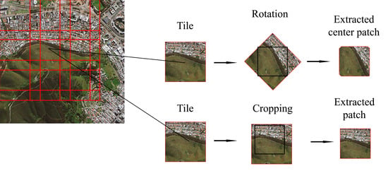
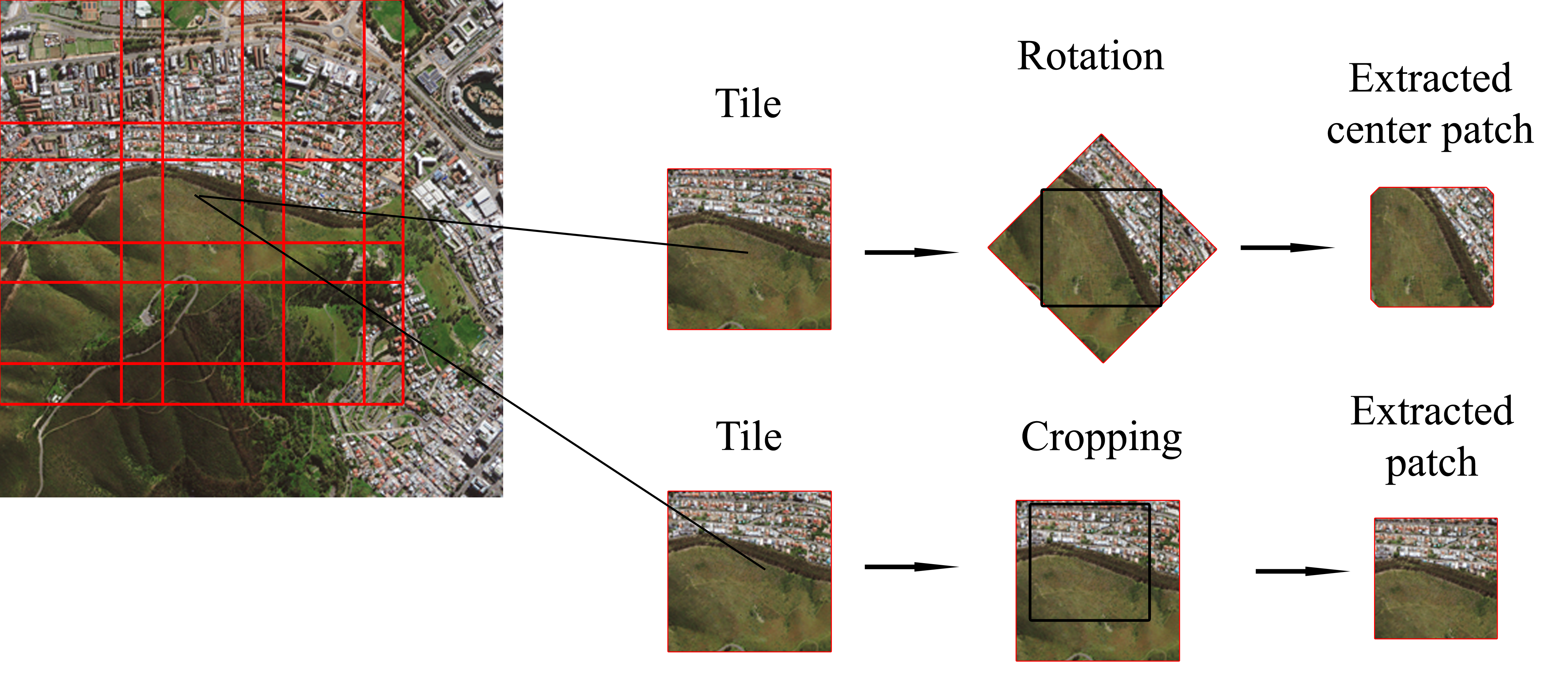
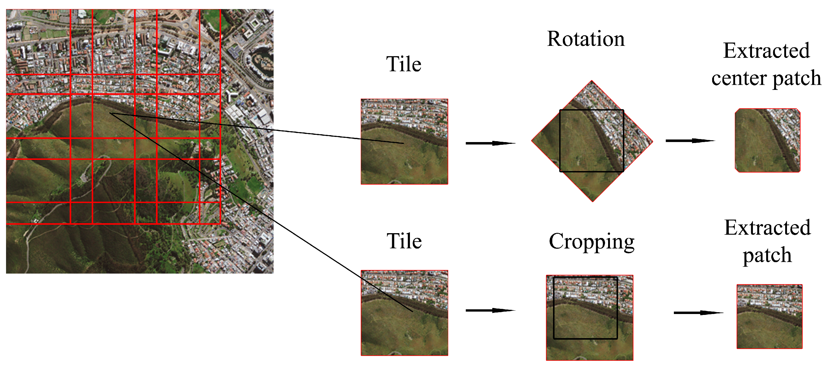
The remote sensing datasets are usually provided in the form of very large images where each image side contains thousands of pixels. However, due to memory constraints, to be able to train the network, we first subdivide the image into smaller tiles. Therefore, as shown in Figure 2, first, each image in the training set is subdivided into tiles of size 364 × 364. Notice that we consider the network input size to be 256 × 256; however, we extract larger tiles to be able to apply a set of augmentation transformations in the course of training as follows. From each tile, with 50% probability, a 256 × 256 patch is cropped at a random position. Otherwise, a 256 × 256 patch is cropped from the center of the tile that has been rotated using a bilinear transformation with a random angle drawn from a uniform distribution in the interval [0, ]. Next, horizontal and vertical flips each with the probability of 50% are applied independently over the extracted patch. Such augmentation techniques are necessary to prevent the network from being overfitted on the training set.
Concerning test images, since no augmentation is planned during the evaluation, we extract tiles of size 256 × 256 with partially overlapping samples from each test image. Averaging the network outputs over overlapped areas and on the neighboring patches helps to avoid artifacts.
2.3. Cost Function and Optimization
After the training and test samples are generated, the network is trained end-to-end in a fully supervised manner minimizing the binary cross-entropy loss function. To be precise, letting be the one-hot target vector corresponding to class k, i.e., only the element corresponding to the correct class is equal to one, whereas all the other elements are equal to zero, then the binary cross-entropy loss function is computed as follows:
where H and W are the input image width and height, respectively, and represents the network parameters. In addition, in order to prevent the network from overfitting on the training samples, the final cost function we actually optimize at training time is:
where is a regularization term defined as the squared L2 norm of all the weights in the network, and and are the learning rate and regularization factor.
We train the network via stochastic gradient descent with the momentum of 0.9 and with the mini-batch size equal to 8. Concerning the learning rate adaptation strategy, we chose a base learning rate of that is divided by a factor of 10 every 100 epochs and we trained the network for a total of 300 epochs. Moreover, L2 regularization with is applied during training.
3. Results
In this section, first we describe the dataset used in this study, then we define the evaluation metrics used to measure the performance; finally, the experiential results are provided.
3.1. Dataset
The dataset used in this study has originally been created by Hughes et al. [34] and is obtained manually from Landsat 8 Operational Land Imager (OLI) scenes. Its purpose was to validate cloud and cloud shadow masking derived from the Spatial Procedures for Automated Removal of Cloud and Shadow (SPARCS) algorithm. The dataset includes 10 spectral bands; however, in most of our experiments, we use only four bands corresponding to red, green, blue and infrared. The annotations are given for seven classes including shadow, shadow over water, water, snow, land, cloud, and flooded areas. In our experiments, we convert such annotations to the binary case of clouds and non-clouds pixels. Eighty images with the size of 1000 by 1000 pixels are provided which we use 80% for training and the remaining 20% for testing. The training and test sets are chosen so that they cover different scenes over different geographical locations. The training set includes 64 images from which 1024 patches (16 patches over each image) of size 364 × 364 have been extracted, and test set includes 16 images from which 256 patches (16 patches over each image) of size 256 × 256 have been extracted.
3.2. Test Metrics
In our experiments, we measure network performance by measuring the following metrics:
- F1-score is defined as the harmonic mean of precision and recall: , where Precision is defined as the ratio of correctly predicted pixels to all predicted pixels regarding a segmentation class: , and Recall is defined as the ratio of correctly predicted pixels to all pixels that belongs to a segmentation class: . Moreover, , and are true positive, false negative and false positive pixels, respectively.
- Overall accuracy is the fraction of correctly labeled pixels for all classes, where and are the number of classes and the number of pixels respectively and denotes true positives for class i.
- mIOU is the ratio of correctly predicted area to the union of predicted pixels and the ground truth which is averaged over all classes.
- Inference memory is the amount of GPU memory, which is occupied by the network during evaluation. The memory consumption is measured based on the maximum allocated GPU memory during inference using a Pytorch implementation of the proposed methodology.
- Computation time considers data loading time, the time interval in which the network processes the extracted patches over a 1000 × 1000 test image, the time needed to stitch patches to form segmentation maps and also the time required to compute the evaluation metrics.
3.3. Experiments
In this section, we provide the experimental results obtained by the network architecture defined in Section 2.1. In order to be able to measure the trade-off between the network resource consumption and its performance on the cloud screening task, we set up several experiments. In these experiments, we use different settings by considering a number of factors that can affect memory consumption as well as the network performance. The factors that are considered include the computation precision, the network encoder depth, the number of convolutional filters, the number of input spectral bands and also the input size. In all experiments, the network is trained from the samples generated over the SPARCS dataset based on the procedure defined in Section 2.2 and employing the training methodology detailed in Section 2.3.
The experimental setup used for all the experiments below consists of running the methodology implemented in Pytorch framework [38] over NVIDIA GeForce GTX 1080 GPU (Santa Clara, CA, United States) with Pascal architecture and 8 GB memory.
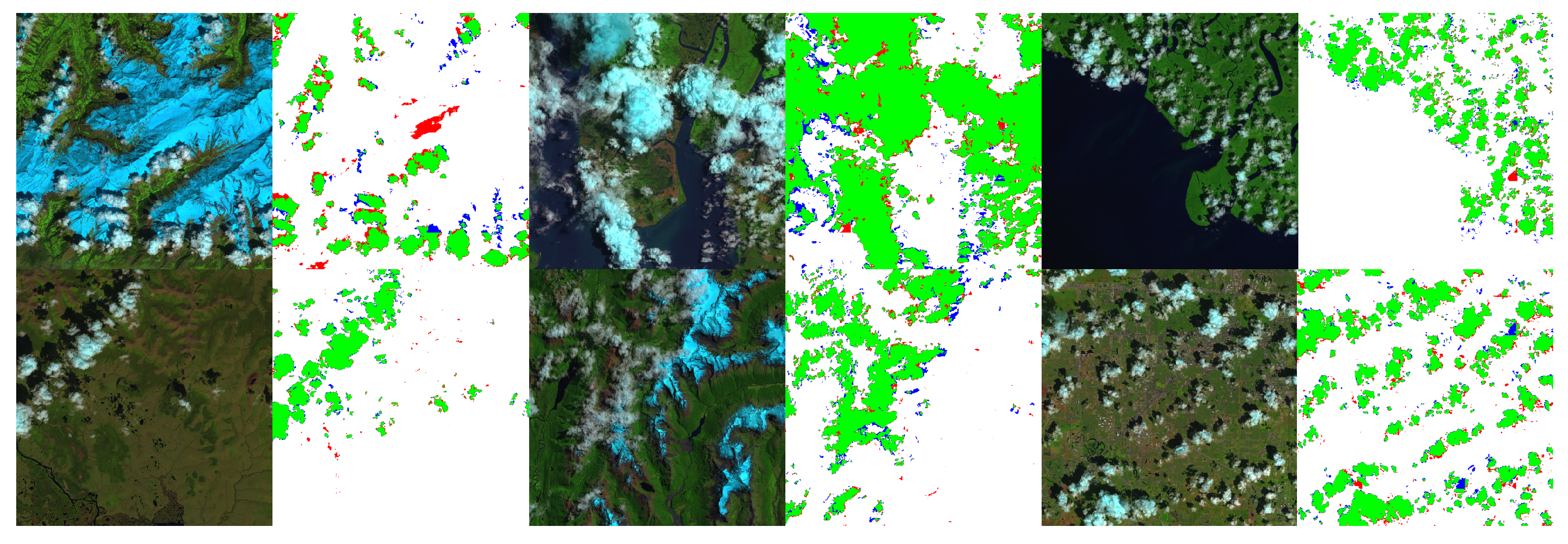
Input bands: In the first experiment, we investigate how the number of spectral bands which are input to the network can affect both the network performance and its memory usage. Therefore, the proposed network defined in Section 2.1 is trained once over four bands of red (R), blue (B), green (G) and infrared (IR) bands, and another time over each one of these bands separately and also once over all 10 bands provided by the SPARCS dataset. As is reported in Table 1, the best results in terms of F1-score, mIOU, and accuracy are obtained when the network is trained over four bands of red, blue, green and infrared. Moreover, it can be seen that, when the network trained over one spectral band, the more informative band is red in terms of overall accuracy and blue in terms of F1-score. We should note that the difference between F1-score and overall accuracy is that the overall accuracy takes into accounts also the true negative pixels; however, F1-score does not consider true negatives. Thus, this explains the variations between overall accuracy and F1-score also in the remaining experiments, where one network may outperform another network only in one metric. Considering the inference, the network with one input band is faster by a small margin of 1 ms in the processing input image (inference time is shown in Table 2) and consumes 2.4 MB less than the network with 10 input bands. The results imply that the number of input spectral bands has a small effect on the network resource consumption since only the number of input channels of the first convolutional layer in the encoder (see Figure 1) changes and the rest of the network remains the same. This also shows that using more than four bands does not bring any improvement to the problem of cloud screening. Figure 3 shows the segmentation results by the network with four input bands and over 6 test images of SPARCS dataset.
Input size: In this experiment, we study the connection between network performance and the input size. Accordingly, we train the proposed network in Section 2.1 over samples that are generated based on the procedure described in Section 2.2, using different sizes for extracting patches i.e., 1000 × 1000, 256 × 256, 128 × 128, and 64 × 64. Since the proposed network is fully convolutional, it can take as input an image with arbitrary size. In all experiments in this part, the four spectral bands corresponding to red, green, blue and infrared are used. The 1st, 7th, 8th, and 9th rows in Table 1 show the results for input size of 256 × 256, 1000 × 1000, 128 × 128 and 64 × 64, respectively; it can be seen that in terms of cloud screening performance, the network with input size of 128 × 128 has the best overall accuracy and mIOU while the network with input size of 256 × 256 performs with the best F1-score. In terms of memory consumption, decreasing the input size from 256 × 256 to 128 × 128 results in releasing about 5.3 MB of the memory, and in terms of inference time (Table 2) it processes the input data 22 ms faster. However, we note that further decreasing the input size contributes only marginally to the memory consumption; however, it can worsen the network performance and also leads to slower inference time due to the larger number of patches that should be extracted to cover the test image. Such performance declines for smaller input size can be related to shrinking the network field of view. Moreover, regarding the input size of 1000 × 1000, as it covers the whole test images, it does not require stitching during inference and hence decreases the processing time. As is mentioned in Section 2.1, the larger the network field of view is, the more neighboring pixels are considered in predicting the score maps. To conclude, smaller input size can decrease the network memory consumption, but this comes at the expense of shrinking the network field of the view that may worsen the overall performance.
Precision: In this experiment, we investigate how the network performance can be influenced by the floating point precision employed for the representation of network parameters and the corresponding computations, hence we experiment with half precision computations. Pytorch framework by default uses full precision floating-point which occupies 32 bits, thus by halving the precision of the floating points, 16 bits will be occupied. In this experiment, we used half-precision floating point both in training and test stages. As Table 1 shows, the network with half-precision (10th row) occupies 8.05 MB of memory. Compared to the network with full precision (1st row) which consumes 15.52 MB, half precision computations leads to releasing about 50% of the memory during inference. Moreover, the network with the half precision processes the input 10 ms faster. However, in terms of segmentation performance, halving the precision results in a considerable drop of 14% in terms of F1-score, 33% in mIOU and 10% in overall accuracy. To conclude, as it will be explored in the next sections, compared with other approaches, halving the precision can be regarded as an expensive approach of managing memory in terms of network segmentation performance.
Convolutional filters: In this part, we consider the number of convolutional filters in the network that can have a significant impact on the network performance. We measure the cloud screening performance and the memory consumption for the network with the same architecture defined in Section 2.1 but with a number of convolutional filters that is divided first by a factor of two (Plain *) and then by a factor of four (Plain ). As reported in Table 1, dividing the number of network filters by a factor of two (11th row) and by a factor of four (12th row) results in 75% and 90% reduction in the number of network parameters, respectively. As a result, the first (Plain *) and second (Plain ) networks consume about 8.5 MB and 11.6 MB less memory during inference compared with the original architecture (1st row). While the performance of the first network (Plain *) drops by 0.28% in F1-score, 0.44% in mIOU and remains approximately the same in terms of overall accuracy, the performance of second network (Plain ) drops by larger margin of 1.46% in F1-score, 2.16 % in mIOU and 0.45% in overall accuracy. Such results imply that, to some extent, reducing the number of convolutional filters within a specific network can reduce the network memory consumption while preserving its performance, but this must not be overdone.
Output scale: In this experiment, to optimize resource consumption, we omit the last decoder block (i.e., fifth block), hence the output scale is halved compared to input patch. As can be seen from the results in Table 1 and Table 2 (denoted by Plain **), this approach can free up the memory by 3.7 MB (23%) and speed up the total processing time by 18 ms while the performance drops only by 1% in F1-score.
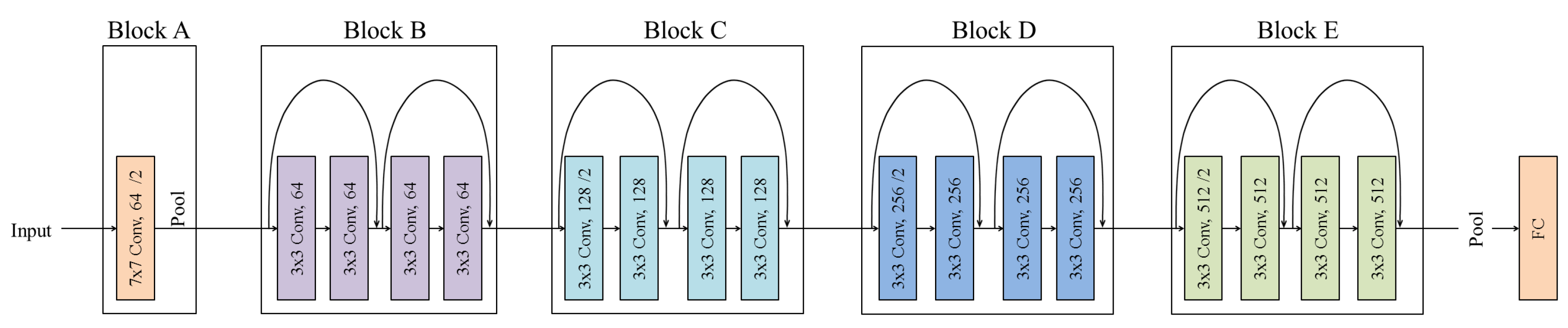
Encoder depth: Finally, we measure how a deeper encoder can improve network performance. It is well known that deeper networks generalize better over large datasets [17]. Moreover, it has been shown that, among deeper networks, residual networks (ResNets) have better generalization ability and can converge faster thanks to the employment of skip connection [18,26]. Hence, in this experiment, we deepen the encoder by using residual networks with 18, 34 and 50 layers in the encoding stage of the proposed network. As a result, the convolution layers in the encoder are replaced by residual blocks as shown in Figure 4 for ResNet-18, while the decoder architecture remains the same. As can be seen from the last three rows in Table 1, the residual encoder brings a considerable improvement in terms of both F1-score and overall accuracy. Using ResNet with 18, 34 and 50 layers as encoder leads to a increase of 2.23%, 2.03% and 1.41% in F1-score, 3.32 %, 2.92 % and 2.09 % in mIOU and 1%, 1.18% and 0.9% in overall accuracy, respectively. However, the number of network parameters grows by a factor of 13, 21 and 81 for ResNet 18, 34 and 50. In terms of inference time for the forward pass, as can be seen from Table 2, using ResNets as encoder leads to an increase by a margin of 239, 368 and 565 ms for depths of 18, 34 and 50 layers, respectively. Therefore, using deeper residual networks can improve cloud detection performance significantly, but it comes at the expense of an increased cost in terms of memory consumption and inference time.
Comparison with state-of-the-art: Finally, we compare the performance of the proposed network with that of Deeplab V3+ [19] which achieved state-of-the-art performance over PASCAL VOC 2012 [40] and Cityscapes [41] datasets. Deeplab V3+ also makes use of encoder–decoder architecture to perform image segmentation. Authors showed in [42] that Deeplab V3+ with ResNet-101 and Xception encoders obtained the best performance. Therefore, we also train Deeplab V3+ once with ResNet-101 and another time with Xception encoder over the SPARCS dataset. As can be seen in the last two rows of Table 1, for the cloud screening task, Deeplab V3+ with ResNet encoder outperforms its variant with Xception encoder by a considerable margin in overall accuracy and F1-score. In terms of memory consumption, comparing Deeplab with our proposed network and both with ResNet as the encoder, Deeplab has fewer parameters and occupies much less memory. This is due to the Deeplab architecture that does not include deconvolutional filters in its decoder and relies on upsampling operations that do not include parameters. Nevertheless, as can be seen from the results, our proposed network with plain encoder (Plain * in Table 1) outperforms Deeplab in both overall accuracy and F1-score while consuming about 71 times less memory. We conjecture that such decrease in Deeplab performance is related to the use of deeper encoder, which makes it prone to overfitting. Analogously, we have noticed a similar decline in our proposed network performance when the encoder becomes larger. For instance, a drop in F1-score and mIOU can be seen in Table 1 by comparing the proposed network with ResNet 18 and 50 as the encoder. In addition to overfitting, we notice that the deconvolutional layers which are used in our network, instead of bilinear upsampling layers in Deeplab, contribute to higher performance, although they increase the number of network parameters. Concerning the processing time, since the upsampling operation in Deeplab decoder is carried out on CPU in Pytorch, Deeplab takes more time compared with our proposed network. In addition to Deeplab V3+, we train the original U-net architecture over the SPARCS dataset. Due to the differences that are highlighted in Section 2.1, U-net consumes about 300 MB more memory during inference compared with our proposed network with plain encoder (1st row); however, it contributes to performance by a margin of 0.65 and 1.36 in F1-score and mIOU, respectively. Nevertheless, considering the proposed network with ResNet18 encoder, it not only outperforms original U-net in performance but also consumes less memory during inference. Moreover, F-mask [39] algorithm is applied over the SPARCS test images using all available 10 bands. As Table 1 reports, CNN based approaches surpass F1-mask by a great margin.
In the end, in Figure 5, learned filters in three convolutional layers of the trained network encoder (plain) and the corresponding feature maps of a sample input are depicted. We select 16 filters and feature maps from each of these three convolutional layers. As can be seen, the feature maps resolution decreases in deeper layers of the encoder while more semantic visual patterns are represented. Regarding the learned filters, since the depth of filters increases in deeper layers, the filters of such layers cannot be visualized properly in RGB. However, in the first convolutional layer, filters have a depth of 3 and hence can be visualized in RGB. Most of these filters have circular shapes, which can be related to the cloud shape, showing that the learned filters represent templates that are effective for detecting clouds.
4. Conclusions
In this study, we addressed the cloud screening problem by considering the hardware constraints imposed by the satellite platforms. We proposed an encoder–decoder CNN to perform pixel-based classification on satellite images, in order to discard images that are highly contaminated by clouds to preserve resources. To enable an onboard implementation, we limit the resource consumption by CNN while preserving its performance by optimizing the network architecture. The results show that the proposed network can outperform the state-of-the-art CNN over the SPARCS dataset while consuming much fewer resources during inference. The memory consumption allows these networks to easily fit in the memory of low-power accelerators for embedded applications. The sustainable throughput depends on the specific accelerator and its integration with the CPU. Our results show that the time needed for the forward pass of the neural network is small on a powerful GPU, whereas a low-power accelerator would require more time. Moreover, a significant amount of time is devoted to data transfers between CPU and GPU; in an onboard implementation, these would be highly dependent on the specific architecture of the processing unit, highlighting the need of careful design.
Author Contributions
Conceptualization, S.G. and E.M.; methodology, S.G. and E.M.; software, S.G.; validation, S.G.; formal analysis, S.G.; investigation, S.G.; resources, E.M.; data curation, S.G. and E.M.; writing–original draft preparation, S.G.; writing–review and editing, E.M.; visualization, S.G.; supervision, E.M.; project administration, E.M.; funding acquisition, E.M.
Funding
This research received no external funding.
Conflicts of Interest
The authors declare no conflict of interest.
References
- Saunders, R.W.; Kriebel, K.T. An improved method for detecting clear sky and cloudy radiances from AVHRR data. Int. J. Remote Sens. 1988, 9, 123–150. [Google Scholar] [CrossRef]
- Zhu, Z.; Woodcock, C.E. Object-based cloud and cloud shadow detection in Landsat imagery. Remote Sens. Environ. 2012, 118, 83–94. [Google Scholar] [CrossRef]
- Griggin, M.; Burke, H.h.; Mandl, D.; Miller, J. Cloud cover detection algorithm for EO-1 Hyperion imagery. In Proceedings of the 2003 IEEE International Geoscience and Remote Sensing Symposium IGARSS’03, Toulouse, France, 21–25 July 2003; Volume 1, pp. 86–89. [Google Scholar]
- Zhang, L.; Huang, X.; Huang, B.; Li, P. A pixel shape index coupled with spectral information for classification of high spatial resolution remotely sensed imagery. IEEE Trans. Geosci. Remote Sens. 2006, 44, 2950–2961. [Google Scholar] [CrossRef]
- Benediktsson, J.A.; Pesaresi, M.; Amason, K. Classification and feature extraction for remote sensing images from urban areas based on morphological transformations. IEEE Trans. Geosci. Remote Sens. 2003, 41, 1940–1949. [Google Scholar] [CrossRef] [Green Version]
- Benediktsson, J.A.; Palmason, J.A.; Sveinsson, J.R. Classification of hyperspectral data from urban areas based on extended morphological profiles. IEEE Trans. Geosci. Remote Sens. 2005, 43, 480–491. [Google Scholar] [CrossRef]
- Huang, X.; Zhang, L. A multidirectional and multiscale morphological index for automatic building extraction from multispectral GeoEye-1 imagery. Photogramm. Eng. Remote Sens. 2011, 77, 721–732. [Google Scholar] [CrossRef]
- Huang, X.; Zhang, L. Morphological building/shadow index for building extraction from high-resolution imagery over urban areas. IEEE J. Sel. Top. Appl. Earth Obs. Remote Sens. 2012, 5, 161–172. [Google Scholar] [CrossRef]
- Fisher, A. Cloud and cloud-shadow detection in SPOT5 HRG imagery with automated morphological feature extraction. Remote Sens. 2014, 6, 776–800. [Google Scholar] [CrossRef]
- Merchant, C.; Harris, A.; Maturi, E.; MacCallum, S. Probabilistic physically based cloud screening of satellite infrared imagery for operational sea surface temperature retrieval. Q. J. R. Meteorol. Soc. 2005, 131, 2735–2755. [Google Scholar] [CrossRef] [Green Version]
- Thompson, D.R.; Green, R.O.; Keymeulen, D.; Lundeen, S.K.; Mouradi, Y.; Nunes, D.C.; Castaño, R.; Chien, S.A. Rapid spectral cloud screening onboard aircraft and spacecraft. IEEE Trans. Geosci. Remote Sens. 2014, 52, 6779–6792. [Google Scholar] [CrossRef]
- Shiffman, S. Cloud Detection From Satellite Imagery: A Comparison Of Expert-Generated and Automatically-Generated Decision Trees. 2004. Available online: www.ntrs.nasa.gov (accessed on 1 February 2019).
- Rossi, R.; Basili, R.; Del Frate, F.; Luciani, M.; Mesiano, F. Techniques based on support vector machines for cloud detection on quickbird satellite imagery. In Proceedings of the 2011 IEEE International Geoscience and Remote Sensing Symposium (IGARSS), Vancouver, BC, Canada, 24–29 July 2011; pp. 515–518. [Google Scholar]
- Wagstaff, K.L.; Altinok, A.; Chien, S.A.; Rebbapragada, U.; Schaffer, S.R.; Thompson, D.R.; Tran, D.Q. Cloud Filtering and Novelty Detection using Onboard Machine Learning for the EO-1 Spacecraft. 2017. Available online: https://ai.jpl.nasa.gov (accessed on 1 February 2019).
- Murino, L.; Amato, U.; Carfora, M.F.; Antoniadis, A.; Huang, B.; Menzel, W.P.; Serio, C. Cloud detection of MODIS multispectral images. J. Atmos. Ocean. Technol. 2014, 31, 347–365. [Google Scholar] [CrossRef]
- Krizhevsky, A.; Sutskever, I.; Hinton, G.E. Imagenet classification with deep convolutional neural networks. In Proceedings of the Advances in Neural Information Processing Systems, Stateline, NV, USA, 3–8 December 2012; pp. 1097–1105. [Google Scholar]
- Szegedy, C.; Liu, W.; Jia, Y.; Sermanet, P.; Reed, S.; Anguelov, D.; Erhan, D.; Vanhoucke, V.; Rabinovich, A. Going deeper with convolutions. In Proceedings of the IEEE Conference on Computer Vision and Pattern Recognition, Boston, MA, USA, 7–12 June 2015; pp. 1–9. [Google Scholar]
- He, K.; Zhang, X.; Ren, S.; Sun, J. Deep residual learning for image recognition. In Proceedings of the IEEE Conference on Computer Vision and Pattern Recognition, Las Vegas, NV, USA, 26–30 June 2016; pp. 770–778. [Google Scholar]
- Chen, L.C.; Papandreou, G.; Kokkinos, I.; Murphy, K.; Yuille, A.L. Deeplab: Semantic image segmentation with deep convolutional nets, atrous convolution, and fully connected crfs. IEEE Trans. Pattern Anal. Mach. Intell. 2018, 40, 834–848. [Google Scholar] [CrossRef]
- He, K.; Gkioxari, G.; Dollár, P.; Girshick, R. Mask r-cnn. In Proceedings of the IEEE International Conference on Computer Vision, Venice, Italy, 22–29 October 2017; pp. 2980–2988. [Google Scholar]
- Ghassemi, S.; Fiandrotti, A.; Caimotti, E.; Francini, G.; Magli, E. Vehicle joint make and model recognition with multiscale attention windows. Signal Process. Image Commun. 2019, 72, 69–79. [Google Scholar] [CrossRef]
- Xu, Y.; Xie, Z.; Feng, Y.; Chen, Z. Road extraction from high-resolution remote sensing imagery using deep learning. Remote Sens. 2018, 10, 1461. [Google Scholar] [CrossRef]
- Arief, H.; Strand, G.H.; Tveite, H.; Indahl, U. Land cover segmentation of airborne LiDAR data using stochastic atrous network. Remote Sens. 2018, 10, 973. [Google Scholar] [CrossRef]
- Panboonyuen, T.; Jitkajornwanich, K.; Lawawirojwong, S.; Srestasathiern, P.; Vateekul, P. Semantic segmentation on remotely sensed images using an enhanced global convolutional network with channel attention and domain specific transfer learning. Remote Sens. 2019, 11, 83. [Google Scholar] [CrossRef]
- Zhu, K.; Chen, Y.; Ghamisi, P.; Jia, X.; Benediktsson, J.A. Deep convolutional capsule network for hyperspectral image spectral and spectral-spatial classification. Remote Sens. 2019, 11, 223. [Google Scholar] [CrossRef]
- Ghassemi, S.; Sandu, C.; Fiandrotti, A.; Tonolo, F.G.; Boccardo, P.; Francini, G.; Magli, E. Satellite image segmentation with deep residual architectures for time-critical applications. In Proceedings of the 26th European Signal Processing Conference, Eternal City, Rome, 3–7 September 2018; pp. 2235–2239. [Google Scholar]
- Ghassemi, S.; Fiandrotti, A.; Francini, G.; Magli, E. Learning and Adapting Robust Features for Satellite Image Segmentation on Heterogeneous Datasets. IEEE Trans. Geosci. Remote Sens. Under review.
- Shi, M.; Xie, F.; Zi, Y.; Yin, J. Cloud detection of remote sensing images by deep learning. In Proceedings of the 2016 IEEE International Geoscience and Remote Sensing Symposium (IGARSS), Beijing, China, 10–15 July 2016; pp. 701–704. [Google Scholar]
- Le Goff, M.; Tourneret, J.Y.; Wendt, H.; Ortner, M.; Spigai, M. Deep learning for cloud detection 2017. Available online: https://hal.archives-ouvertes.fr (accessed on 1 February 2019).
- Wu, X.; Shi, Z. Utilizing multilevel features for cloud detection on satellite imagery. Remote Sens. 2018, 10, 1853. [Google Scholar] [CrossRef]
- Zhaoxiang, Z.; Iwasaki, A.; Guodong, X.; Jianing, S. Small Satellite Cloud Detection Based on Deep Learning and Image Compression. Available online: www.preprints.org (accessed on 1 February 2019 ).
- Ronneberger, O.; Fischer, P.; Brox, T. U-net: Convolutional networks for biomedical image segmentation. In Proceedings of the International Conference on Medical Image Computing and Computer–Assisted Intervention, Munich, Germany, 5–9 October 2015; Springer: Cham, Switherland, 2015; pp. 234–241. [Google Scholar]
- Mohajerani, S.; Krammer, T.A.; Saeedi, P. A Cloud Detection Algorithm for Remote Sensing Images Using Fully Convolutional Neural Networks. In Proceedings of the 2018 IEEE 20th International Workshop on Multimedia Signal Processing (MMSP), Vancouver, BC, Canada, 29–31 August 2018; pp. 1–5. [Google Scholar]
- Hughes, M.J.; Hayes, D.J. Automated detection of cloud and cloud shadow in single-date Landsat imagery using neural networks and spatial post-processing. Remote Sens. 2014, 6, 4907–4926. [Google Scholar] [CrossRef]
- U.S. Geological Survey, L8 SPARCS Cloud Validation Masks. U.S. Geological Survey Data Release 2016. United States Geological Survey (Reston, Virginia, United States). Available online: www.usgs.gov (accessed on 1 February 2019).
- Francis, A.; Sidiropoulos, P.; Vazquez, E. Real-Time Cloud Detection in High-Resolution Videos: Challenges and Solutions. In Proceedings of the Onboard Payload Data Compression Workshop, Matera, Italy, 20–21 September 2018. [Google Scholar]
- Long, J.; Shelhamer, E.; Darrell, T. Fully convolutional networks for semantic segmentation. In Proceedings of the IEEE Conference on Computer Vision and Pattern Recognition, Boston, MA, USA, 7–12 June 2015; pp. 3431–3440. [Google Scholar]
- Paszke, A.; Gross, S.; Chintala, S.; Chanan, G.; Yang, E.; DeVito, Z.; Lin, Z.; Desmaison, A.; Antiga, L.; Lerer, A. Automatic differentiation in PyTorch. 2017. Available online: www.pytorch.org (accessed on 1 February 2019).
- Zhu, Z.; Wang, S.; Woodcock, C.E. Improvement and expansion of the Fmask algorithm: Cloud, cloud shadow, and snow detection for Landsats 4–7, 8, and Sentinel 2 images. Remote Sens. Environ. 2015, 159, 269–277. [Google Scholar] [CrossRef]
- Everingham, M.; Eslami, S.A.; Van Gool, L.; Williams, C.K.; Winn, J.; Zisserman, A. The pascal visual object classes challenge: A retrospective. Int. J. Comput. Vis. 2015, 111, 98–136. [Google Scholar] [CrossRef]
- Cordts, M.; Omran, M.; Ramos, S.; Rehfeld, T.; Enzweiler, M.; Benenson, R.; Franke, U.; Roth, S.; Schiele, B. The cityscapes dataset for semantic urban scene understanding. In Proceedings of the IEEE Conference on Computer Vision and Pattern Recognition, Las Vegas, NV, USA, 27–30 June 2016; pp. 3213–3223. [Google Scholar]
- Encoder-decoder with atrous separable convolution for semantic image segmentation. In Proceedings of the European Conference on Computer Vision, Munich, Germany, 8–14 September 2018; pp. 833–851.
Figure 1.
Network architecture: the encoder (bottom) and the decoder (top) are illustrated in dashed boxes. Number of input and output channels (i.e., feature maps) as well as the size of filter, stride and padding are provided for each layer.
Figure 1.
Network architecture: the encoder (bottom) and the decoder (top) are illustrated in dashed boxes. Number of input and output channels (i.e., feature maps) as well as the size of filter, stride and padding are provided for each layer.

Figure 2.
Patch extraction and data augmentation during training.

Figure 3.
The results of the proposed network (1-st row in Table 1) over six test images of SPARCS dataset. Green and white pixels represent true positive and true negative while blue and red pixels represent false negative and false positive outputs, respectively.
Figure 3.
The results of the proposed network (1-st row in Table 1) over six test images of SPARCS dataset. Green and white pixels represent true positive and true negative while blue and red pixels represent false negative and false positive outputs, respectively.

Figure 4.
ResNet with 18 layers depicted in five blocks.

Figure 5.
Learned convolutional filters (bottom) and corresponding feature maps (top) for a sample input patch (left).
Figure 5.
Learned convolutional filters (bottom) and corresponding feature maps (top) for a sample input patch (left).


Table 1.
The proposed network performance is provided (top) with different encoder networks, encoder depths, computation precision, input spatial and spectral sizes. Moreover, the performance of state-of-the-art CNN, namely DeepLab V3+, is provided as well (bottom) with two different encoders.
Table 1.
The proposed network performance is provided (top) with different encoder networks, encoder depths, computation precision, input spatial and spectral sizes. Moreover, the performance of state-of-the-art CNN, namely DeepLab V3+, is provided as well (bottom) with two different encoders.
| Encoder | Precision | Input Bands | Input Size [Pixels] | Number of Parameters | Inference Memory [MB] | Overall Accuracy [%] | F1-Score [%] | mIOU [%] | |
|---|---|---|---|---|---|---|---|---|---|
| Type | Depth | ||||||||
| Plain | 5 | full | R,B,G,IR | 256 × 256 | 1,269,018 | 15.52 | 95.24 | 90.36 | 83.53 |
| Plain | 5 | full | R | 256 × 256 | 1,266,666 | 14.72 | 94.51 | 87.99 | 80.37 |
| Plain | 5 | full | B | 256 × 256 | 1,266,666 | 14.72 | 94.36 | 88.27 | 80.55 |
| Plain | 5 | full | G | 256 × 256 | 1,266,666 | 14.72 | 94.06 | 87.25 | 79.30 |
| Plain | 5 | full | IR | 256 × 256 | 1,266,666 | 14.72 | 92.38 | 85.15 | 76.08 |
| Plain | 5 | full | All | 256 × 256 | 1,273,722 | 17.11 | 95.15 | 90.22 | 83.49 |
| Plain | 5 | full | R,B,G,IR | 1000 × 1000 | 1,269,018 | 188.60 | 95.18 | 90.01 | 83.43 |
| Plain | 5 | full | R,B,G,IR | 128 × 128 | 1,269,018 | 10.20 | 95.46 | 90.06 | 83.55 |
| Plain | 5 | full | R,B,G,IR | 64 × 64 | 1,269,018 | 9.20 | 95.27 | 89.16 | 82.39 |
| Plain | 5 | half | R,B,G,IR | 256 × 256 | 1,269,018 | 8.05 | 85.06 | 75.45 | 55.49 |
| Plain * | 5 | full | R,B,G,IR | 256 × 256 | 318,478 | 7.03 | 95.28 | 90.08 | 83.09 |
| Plain | 5 | full | R,B,G,IR | 256 × 256 | 80,232 | 3.87 | 94.79 | 88.90 | 81.37 |
| Plain ** | 5 | full | R,B,G,IR | 256 × 256 | 1,264,946 | 11.83 | 95.05 | 89.40 | 82.39 |
| ResNet | 18 | full | R,B,G,IR | 256 × 256 | 16,550,722 | 132.56 | 96.24 | 92.59 | 86.85 |
| ResNet | 34 | full | R,B,G,IR | 256 × 256 | 26,658,882 | 267.23 | 96.42 | 92.39 | 86.45 |
| ResNet | 50 | full | R,B,G,IR | 256 × 256 | 103,629,954 | 889.29 | 96.23 | 91.77 | 85.62 |
| U-net | 9 | full | R,B,G,IR | 256 × 256 | 39,402,946 | 315.36 | 96.08 | 91.01 | 84.89 |
| FMask | - | full | All | 1000 × 1000 | - | - | 86.81 | 70.11 | 62.01 |
| Deeplab V3+ | |||||||||
| ResNet | 101 | full | R,B,G,IR | 256 × 256 | 59,342,562 | 503.7 | 94.87 | 89.47 | 82.07 |
| Xception | - | full | R,B,G,IR | 256 × 256 | 54,700,722 | 481.69 | 89.85 | 83.58 | 73.51 |
* number of filters divided by two; number of filters divided by four; ** the last decoder block is omitted.
Table 2.
The time interval which is required to (a) load the extracted patches (over 1000 × 1000 pixels test image) from hard drive into memory; (b) compute the network outputs over the input patches (i.e., patches extracted from a test image); (c) stitch the network outputs (to produce 1000 × 1000 segmentation maps); and (d) compute the evaluation metrics is provided.
| Encoder | Precision | Input Bands | Input Size [Pixels] | Data Loading [ms] | Inference [ms] | Stitch [ms] | Eval Metrics [ms] | Total [ms] | |
|---|---|---|---|---|---|---|---|---|---|
| Type | Depth | ||||||||
| Plain | 5 | full | 4 | 256 × 256 | 37 | 168 | 110 | 415 | 730 |
| Plain | 5 | full | 1 | 256 × 256 | 8 | 167 | 110 | 415 | 700 |
| Plain | 5 | full | 10 | 256 × 256 | 7240 | 170 | 110 | 415 | 7935 |
| Plain | 5 | full | 4 | 1000 × 1000 | 17 | 171 | 0 | 415 | 603 |
| Plain | 5 | full | 4 | 128 × 128 | 45 | 146 | 110 | 415 | 716 |
| Plain | 5 | full | 4 | 64 × 64 | 80 | 1136 | 110 | 415 | 1741 |
| Plain | 5 | half | 4 | 256 × 256 | 18 | 158 | 110 | 415 | 701 |
| Plain * | 5 | full | 4 | 256 × 256 | 37 | 153 | 110 | 415 | 715 |
| Plain | 5 | full | 4 | 256 × 256 | 37 | 100 | 110 | 415 | 662 |
| Plain ** | 5 | full | 4 | 256 × 256 | 37 | 150 | 110 | 415 | 712 |
| ResNet | 18 | full | 4 | 256 × 256 | 37 | 407 | 110 | 415 | 969 |
| ResNet | 34 | full | 4 | 256 × 256 | 37 | 536 | 110 | 415 | 1098 |
| ResNet | 50 | full | 4 | 256 × 256 | 37 | 733 | 110 | 415 | 1295 |
| U-net [32] | 9 | full | 4 | 256 × 256 | 37 | 720 | 110 | 415 | 1282 |
| FMask [39] | - | full | 10 | 1000 × 1000 | 37 | 1470 | - | 415 | 1922 |
| Deeplab V3+ | |||||||||
| ResNet | 101 | full | 4 | 256 × 256 | 37 | 422 | 110 | 415 | 984 |
| Xception | - | full | 4 | 256 × 256 | 37 | 441 | 110 | 415 | 1003 |
* number of filters divided by two; number of filters divided by four; ** the last decoder block is omitted.
© 2019 by the authors. Licensee MDPI, Basel, Switzerland. This article is an open access article distributed under the terms and conditions of the Creative Commons Attribution (CC BY) license (http://creativecommons.org/licenses/by/4.0/).
Share and Cite
MDPI and ACS Style
Ghassemi, S.; Magli, E. Convolutional Neural Networks for On-Board Cloud Screening. Remote Sens. 2019, 11, 1417. https://0-doi-org.brum.beds.ac.uk/10.3390/rs11121417
AMA Style
Ghassemi S, Magli E. Convolutional Neural Networks for On-Board Cloud Screening. Remote Sensing. 2019; 11(12):1417. https://0-doi-org.brum.beds.ac.uk/10.3390/rs11121417
Chicago/Turabian StyleGhassemi, Sina, and Enrico Magli. 2019. "Convolutional Neural Networks for On-Board Cloud Screening" Remote Sensing 11, no. 12: 1417. https://0-doi-org.brum.beds.ac.uk/10.3390/rs11121417
Note that from the first issue of 2016, this journal uses article numbers instead of page numbers. See further details here.