Relating X-band SAR Backscattering to Leaf Area Index of Rice in Different Phenological Phases

Abstract

The objective of this study is to provide complete information on the dynamic relationship between X-band (3.11 cm) backscattering intensity (σ°) and rice crop’s leaf area index (LAI) at all growth phases. Though the relationship between X-band σ° and LAI has been previously explored, details on the relationship at the reproductive phase remain unstudied. LAI at the reproductive phase is important particularly at the heading stage where LAI reaches its maximum as it is closely related to grain yield, and at flowering stage where the total leaf area affects the amount of photosynthates. Therefore, this study examined the relationship of increasing LAI (vegetative to reproductive phase) and decreasing LAI (ripening phase) with TerraSAR-X (TSX) ScanSAR (3.11 cm) σ° at HH polarisation and 45° incidence angle. The results showed a statistically significant (R² = 0.51, p value < 0.001) non-linear relationship of LAI with σ° at the vegetative to reproductive phase while no significant linear relationship was found at the ripening phase. This study completes the response curve of X-band σ° to LAI by filling in the information on the reproductive phase which more accurately characterises the dynamic relationship between the rice crop’s LAI and X-band’s σ°. This contributes to improved knowledge on the use of X-band data for estimating LAI for the whole crop cycle which is essential for the modelling of crop growth and estimation of yield.

1. Introduction

Leaf area index (LAI) is derived from the measurements of how fast radiation is attenuated as it passes through the canopy [1] and this accounts for the leaf surface that intercepts incoming radiation [2,3]. LAI is widely used in the research of photosynthesis [4], crop growth analysis and estimation of crop yield [5,6]. The assimilation of LAI as a state variable in crop growth simulation models (CGSM) has been increasingly used for yield estimation [7]. Many CGSM are point-based and scaling this up to estimate yields across larger areas is an active research field [8,9,10]. Remote sensing can be used to estimate LAI, plant height and phenology, and provides spatial and temporal information on other crop growth parameters [11,12] which can reduce spatial variation and uncertainty [9] resulting in more accurate yield estimates across large areas [8]. This makes the study of the relationship between remote sensing information and LAI a focus for many remote sensing studies [5,13].

LAI can be estimated from remotely sensed data by using empirical or physical approaches. Empirical approaches use statistical techniques to establish a relationship between in situ obtained data and remote sensing-based data [14]. Alternatively, physical-based approaches describe the interaction between radiation, canopy elements and soil surface, which makes it suitable for retrieval of plant variables such as LAI [5,15]. However, the use of a physical model for the retrieval of biophysical variables from microwave data through inversion remains a challenge. This can be attributed to: (i) insufficient modelling of the backscattering within a canopy specifically during panicle initiation; (ii) the large number of input parameters on a 3D structure; (iii) electromagnetic characteristics and biophysical variables (e.g., LAI, biomass and fPAR) required to run the model; and (iv) the limitations inherent in the complex multi-variable model inversion [16]. The random effects of surface water on backscatter and orientation of crop structure are additional factors that pose a challenge in physical modelling.

Radar backscattering behaviour is dependent on the wavelength or frequency, crop structure, dielectric properties of the canopy, physical properties of underlying soil, the relationship of the target with the polarisation state and the target’s angular relationship to the radar illumination angle (incidence angle) [17]. The radar backscatter due to surface scattering is generally strong at lower incidence angles while backscattering due to volume scattering from a heterogeneous surface with low dielectric constant is more uniform at all incidence angles [18].

For X-band (2.4–3.8 cm), backscatter at all incidence angles is sensitive enough to detect the emergence of rice seedlings, and the polarimetric response of rice for HH and VV is quite similar (for all incidence angles) at certain growth phases [19]. There is low backscattering at the initial stage when the rice fields are flooded. Then around tillering stage, a sharp peak occurs followed by a decrease in backscatter for both co-polarisations (more evident in VV than in HH) towards the end of the season [11,19]. In general, it was observed that the dynamic range of the evolution at both HH and VV polarisation as a function of rice crop development is larger for shallow angles than for steep angles [19].

Previous studies that used empirical approaches to examine the relationship of rice backscattering intensity (σ°) with LAI used different combination of frequency bands (Ka, Ku, X, C and L), polarisations (HH, VV, HV and VH) and incidence angles (e.g., 25°, 45°, 50°) (

Table 1. Summary of studies over the years on the relationship of rice crop’s leaf area index (LAI) with Ka, Ku and X-band backscattering intensity (σ°).

Frequency Band	Sensor	Wavelength (cm)	Incident Angle (◦)	Polarisation	Spatial Resolution/Antenna Height (m)	Temporal Resolution (days)	Growth Phase Studied	Relationship with LAI	R2	Sample Size	Source
Ka	scatterometer	1.18	25°, 35°, 45°, 55°	HH, HV, VV, and VH	5 m height	Daily	Transplanting to harvest	Poor correlation	<0.7	not mentioned	Inoue et al., 2002 [22]
Ku	scatterometer	1.88	25°, 35°, 45°, 55°	HH, HV, VV, and VH	5 m height	Daily	Transplanting to harvest	Poor correlation	<0.7	not mentioned	Inoue et al., 2002 [22]
X	scatterometer	3.12	25°, 35°, 45°, 55°	HH, HV, VV, and VH	5 m height	Daily	Transplanting to harvest	Poor correlation	<0.7	not mentioned	Inoue et al., 2002 [22]
X	scatterometer	3.11	20°–60°	HH, HV, VV, and VH	4.16 m height	not mentioned	Before transplanting to late maturing stage	Poor correlation	not mentioned	not mentioned	Kim et al., 2008 [20]
X	COSMO-SkyMed (Spotlight mode)	3.11	54°	VV	1	Single image acquired	Late maturing stage	Poor correlation	0.0064	58	Inoue et al., 2012 [13]
X	TSX and CSK (Spotlight mode)	3.11	44°, 50°, 55°	VV	1.7 x 1.48 and 1 x 1 respectively	Once per season	Transplanting and late maturing stage	Poor correlation (maturing stage)	−0.21 (maturing stage)	128	Inoue et al, 2014 [23]
X	CSK (ScanSAR Wide Region mode)	3.11	45°	HH	30	16	Between transplanting and heading stage	Statistically significant correlation	0.34 (r = 0.58, p < 0.001)	30	Hirooka et al. 2015 [24]

and

Table 2. Summary of studies over the years on the relationship of rice crop’s LAI with C and L-band backscattering intensity (σ°).

Frequency Bands	Sensor	Wavelength (cm)	Incident Angle (◦)	Polarisation	Spatial Resolution/Antenna Height (m)	Temporal Resolution (days)	Growth Phase Studied	Relationship with LAI	R2	Sample Size	Source
C	scatterometer	5.21	25°, 35°, 45°, 55°	HH, HV, VV, and VH	5 m height	Daily	Transplanting to harvest	Best correlated with LAI at HH and HV	0.96–0.97	not mentioned	Inoue et al., 2002 [22]
C	scatterometer	5.66	20°–60°	HH, HV, VV, and VH	4.16 m height	not mentioned	Before transplanting to late maturing stage	Strong correlation at HH and HV at > 45°	0.88–0.94	not mentioned	Kim et al., 2008 [20]
C	ENVISAT ASAR	5.62	31°–39°	VV/HH	30	Image acquired at selected growth stages	Seedling to maturing stage	Strongest correlation at seedling stage	0.62–0.88	32	Chen et al., 2009 [21]
C	Radarsat-2	5.4	28°–37°	HH, HV, VH, VV, HH/VV, HV/HH	not mentioned	Image acquired for two years for important growth stages	Tillering to maturing stage	Strongest correlation at HV and HH/VV	0.88 and 0.84	14 and 20 per growth stage	Kumar et al., 2013 [26]
C	Radarsat-2	5.55	25°–35°	VH	1 × 1	Image acquired at selected growth stages	Vegetative to ripening	Strong correlation	0.84–0.85	41, 52, 12, 24 (2009–2012 respectively)	Inoue et al., 2014 [16]
L	scatterometer	23.79	25°, 35°, 45°, 55°	HH, HV, VV, and VH	5 m height	Daily	Transplanting to harvest	High correlation but only second best compared to C-band	0.88–0.91	not mentioned	Inoue et al., 2002 [22]
L	scatterometer	23.61	20°–60°	HH, HV, VV, and VH	4.16 m height	not mentioned	Before transplanting to late maturing stage	Strong correlation at HH and 50°	0.94	not mentioned	Kim et al., 2008 [20]

).

C-band (3.8–7.5 cm) σ° was found to be significantly and consistently correlated with LAI throughout all rice growth stages [16,20,21] and in most C-band configurations: 25° HH, 25° and 35° for cross-polarisations HV and VH (R² = 0.96–0.97), respectively [22]. L-band (15–30 cm) σ° also has a high correlation with LAI [20] but is just second to C-band (R² = 0.88–0.91) [22]. The availability of free Sentinel 1 (C-band) SAR images since 2014 at a 12-day interval with cross and co-polarisation, make it possible to regularly monitor rice areas and extract biophysical parameters such as LAI at all growth stages.

For the high frequency bands, Ka (0.75–1.1 cm), Ku (1.67–2.4 m) and X-band, σ° was found to have a poor correlation with LAI when the data that covered the whole rice growing period (transplanting to harvest) was used in the correlation analysis [20,22]. However, at the early vegetative phase in the month after transplanting, the backscatter coefficient from high frequency bands was found to increase with increasing LAI when it is <1.5. While at the ripening stage, there is a poor correlation between X-band σ° and LAI [13,20,23]. In a more recent study of Hirooka et al. [24], a significant correlation (r = 0.58, p < 0.001) was found between X-band σ° (HH at 45°) and LAI which was measured and collected four times before the heading stage. The LAI measurements partially covered the reproductive phase [24] and did not provide complete information on the relationship of LAI with X-band σ° at this growth phase (Table 1).

The reproductive phase is particularly important specifically at the heading to flowering stages when LAI is at its maximum and has a strong effect on the amount of available photosynthates which is closely related to grain production [25]. Considering this, our objective is to provide a complete response curve of LAI to X-band σ° with this configuration: 3.11 cm wavelength, HH polarisation and 45° incidence angle. The dynamic relationship during the vegetative to reproductive phase when LAI is increasing, and at the ripening phase when LAI is decreasing was examined using an empirical approach. This could further help characterise and understand the rice crop’s LAI when using X-band.

2. Materials and Methods

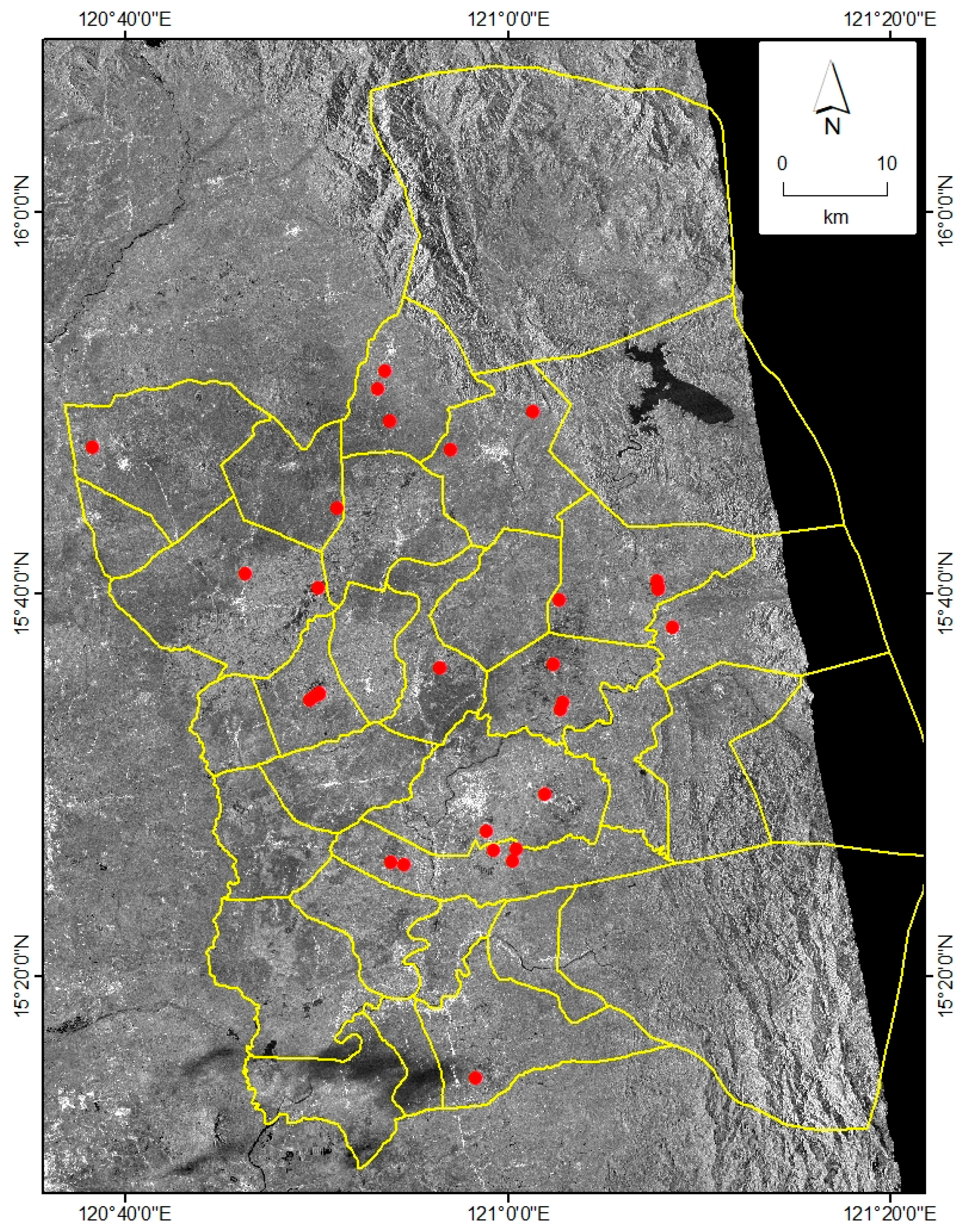
2.1. Study Area

Nueva Ecija (Figure 1) is the largest province of the Central Luzon region of the Philippines. Its land cover is dominated by rice which is mainly grown on alluvial plains and terraces. The province is the leading rice producer of the country [27]. The province has four major rivers: Malimba, Talavera, Chico and Pampanga (the largest) which are the main sources of the Pantabangan reservoir [28]. With these water resources, Nueva Ecija has the highest harvested irrigated rice area among all rice producing provinces in the Philippines: 290,864 ha in 2017 [29]. The total harvested area in 2017 was 324,042 ha, with a total rice production of 1.88 million MT [29].

The province has a distinct dry season (DS) from December to May and wet season (WS) from June to November [30]. In general, the irrigated rice fields are cropped twice a year, once during the WS from June to October, and again in the DS from December to April. Fields are generally kept fallow in May and November though some farmers may plant a green cover crop, like mungbean, which fixes nitrogen and provides a small yield of beans. In terms of crop management, rice is generally transplanted when grown in the WS and directly seeded when grown in the DS [31]. Farmers generally plant rice varieties with a 110 to 115-day crop growth duration.

2.2. TerraSAR-X ScanSAR: Multitemporal Image Acquisition and Processing

TerraSAR-X (TSX) is a satellite operated by the German Aerospace Center (DLR) which became operational in 2008. TSX ScanSAR images (at wavelength 3.11 cm) during the 2013 WS from 8 July–23 September were ordered, however, due to higher priority requests from other users, two of these images (10 and 21 August 2013) were not acquired. Hence, only six images were used in this study to capture the vegetative to ripening phases of rice in Nueva Ecija. The multitemporal TSX ScanSAR images have a spatial resolution of 18.5 m at 45° incidence angle, HH polarisation and 11-day temporal resolution. HH polarisation was chosen because it responds more to the vertical structure of rice plants [20,22]. The double bounce effect between the horizontal flooded field surface and the generally vertical rice plants is more prominent in HH and gives higher backscatter than the VV polarisation [33]. A large incidence angle (45°) was used because it reduces wind effects on water during land preparation prior to transplanting, results in a larger dynamic range of radar backscatter and produces higher spatial resolution [34].

The full description of processing steps for TSX ScanSAR images can be found in [31]. MAPscape-RICE^® [35], a semi-automated software developed by sarmap was used to generate a terrain geocoded σ° by following this processing sequence: (i) multi-looking to reduce speckle and to obtain square pixels; (ii) orbital correction using the SRTM 90 m digital elevation model (DEM); (iii) co-registration of multi-temporal images by gross shift estimation using the orbital data; (iv) De Grandi time-series filtering to achieve a balance in the reflectivity between images acquired at different times using an optimum weighting filter; and (v) terrain geocoding, radiometric calibration and normalization. The σ° allows comparison of radar images acquired at different times, from different sensors or different viewing geometries [31]. The σ° from the multi-temporal images were analysed together with in situ LAI measurements from vegetative to ripening phases.

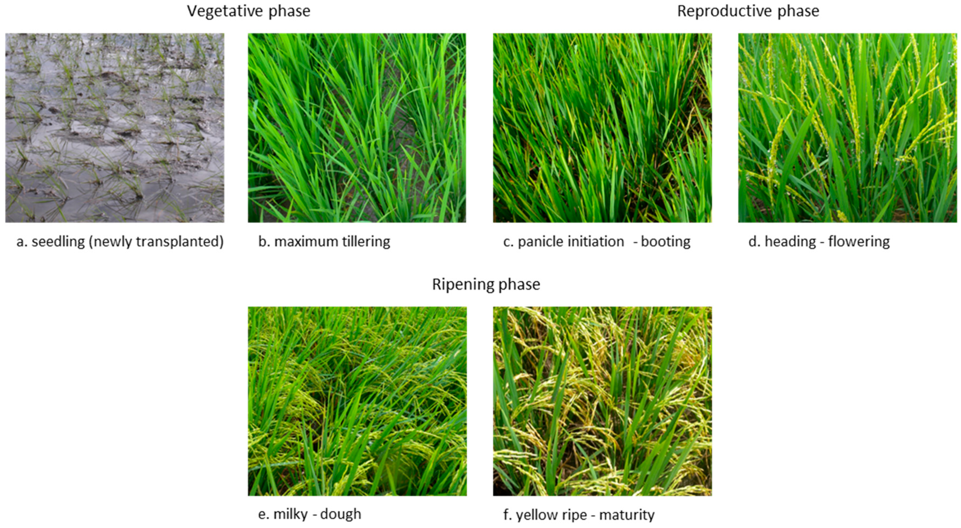
2.3. Monitoring of Sites and Field Data Collection

Field data collection and monitoring of rice fields were carried out during the 2013 WS from 8 July to 23 September on or near to the dates of TSX ScanSAR image acquisitions. A rice-based cropping system map derived from the unsupervised classification of MODIS data from 2006 to 2011 [31] was used as the strata for stratified random sampling to identify the location of rice field monitoring sites [31] for ground data collection (Figure 1). The time needed to complete all observations and plant measurements, the travel time to go from one field to another, budget, person-days, labour constraints and proximity to roads were all considered in determining the number of monitoring sites. Pre-tests of the questionnaire and data collection form were carried out to further determine the feasible number of sites for this study [31]. This resulted in a final selection of 30 monitoring sites located in 13 municipalities of Nueva Ecija. The dates of sowing, transplanting and harvesting were recorded for each site through farmers’ interviews. Transplanting and harvesting dates in the monitored rice fields varied considerably over a two-month period from 8 June to 5 August and from 5 September to 5 November 2013, respectively.

Other field data collected at each monitoring site during or near each satellite pass included in situ LAI, rice crop growth stage, rice variety, water depth and observed weather conditions (e.g., rainy, cloudy, sunny). Secondary daily rainfall data was also acquired from the Tropical Rainfall Measurement Mission (TRMM) 3B42 product [36]. Figure S1 shows the actual data collection form.

2.4. In situ LAI Measurement

In situ LAI measurements were carried out with three replications for each monitoring site every 11 days from 8 July to 23 September 2013, synchronised with Terra SAR-X (TSX) ScanSAR image acquisition dates (±1–2 days). An AccuPAR LP-80 ceptometer was used for the in situ LAI measurements. The photosensors measure photosynthetically active radiation (PAR) in the spectrum that plants use for photosynthesis, i.e., from 400–700 nm. LAI was calculated based on the above and below canopy PAR measurements which were simultaneously measured through the use of an external PAR sensor provided with the AccuPAR. Other variables (zenith angle, fractional beam measurement value, and leaf area distribution parameter) related to the canopy and position of the sun were also automatically calculated [37]. The 30 rice fields that were monitored were planted at different dates, hence, had varying growth stages at the time of the 8 July image acquisition, resulting in a different number of in situ LAI measurements for each monitored site by 23 September 2013.

The identification of rice growth phases and stages during monitoring was based on the International Rice Research Institute’s (IRRI) classification of rice plant growth. The vegetative phase is subdivided into three stages: germination, seedling and tillering (maximum tillering and stem elongation); the reproductive phase is subdivided into panicle initiation, booting, heading and flowering; and the ripening phase into milky, dough, yellow ripe and maturity [25,38]. In a tropical country like the Philippines, a 120-day rice variety will have approximately 60 days, 30 days and 30 days for the vegetative, reproductive and ripening phases respectively [38]. Figure 2 shows photos of a rice field monitored at various crop growth stages during different observation dates throughout the season.

2.5. Interpolation of LAI (from the in situ LAI Measurements)

For each monitored site, the in situ LAI measurements were interpolated to derive the best LAI estimate at the date of image acquisition. This allowed: (i) the estimation of LAI on the dates of image acquisition where in situ measurements are not available; (ii) estimation of dates at the heading/flowering stage where LAI reaches its peak; and (iii) removal of noise in the individual observations. The semi-mechanistic LAI model of Baret [15,39,40] was used for the LAI interpolation (Equation (1)).

$$LAI=LA{I}_{amp} \left\{\frac{1}{1+ex{p}^{-b\left(T-T_i\right)}}-ex{p}^{-a\left(T-T_s\right)}\right\}$$

(1)

Baret’s model [40] splits the LAI dynamics into growth and senescence. In the equation, T is the accumulated daily mean air temperature above 8 °C starting from sowing date and LAI_amp is the amplitude of the maximal leaf area [40]. The growth period is based on a logistic equation which describes the dynamics before the time of maximum LAI, with parameter b as the relative growth rate at the inflexion point Ti. The senescence period is based on an exponential equation describing the period after maximum LAI, with parameter a as the relative growth rate and Ts as the time expressed in temperature with senesced leaves. For each site: b, T_i, a, T_s and LAI_amp were estimated by selecting the combination delivering the lowest RMSE value when compared to all in situ data. The temperature data used as input for Baret’s model was acquired from NASA POWER Climatology Resource for Agroclimatology [41]. In situ LAI data were measured from the monitored fields, whereas, sowing and harvesting dates were acquired through farmers’ interviews.

2.6. Analysis of the Relationship of Backscatter Coefficient (σ°) and LAI

The maximum LAI occurs during the heading–flowering stage of the rice crop [4]. This study investigated how σ° relates to the increasing (vegetative to reproductive phase) and decreasing LAI (ripening phase). A scatter plot was used to get an overview of the overall pattern of the relationship: the direction (positive, negative or neither), the form (linear or non-linear) and the strength (strong or weak based on how close the data points follow the form) [42]. Based on this, a third order polynomial regression was chosen to approximate the non-linear relationship of σ° with LAI.

3. Results

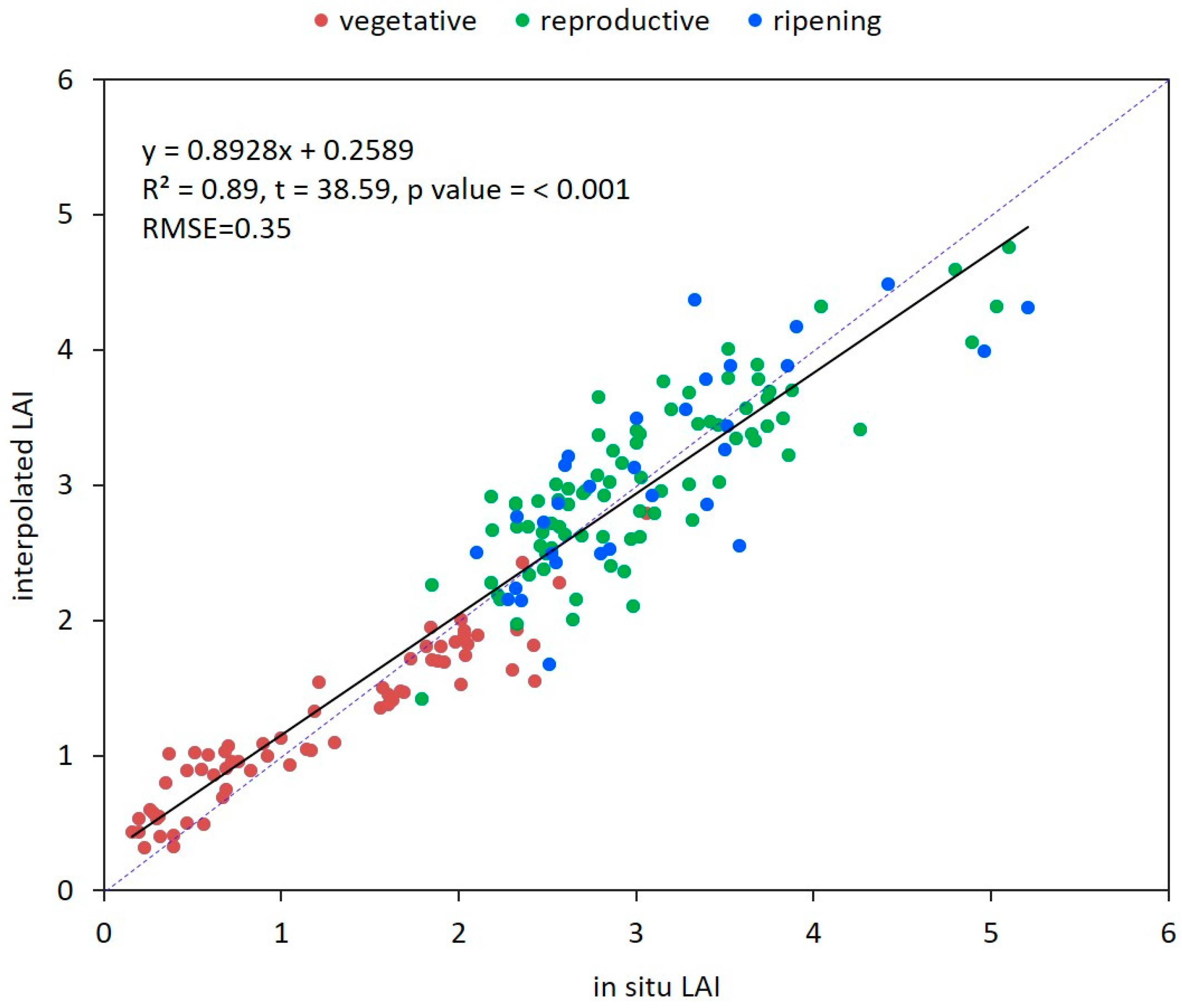
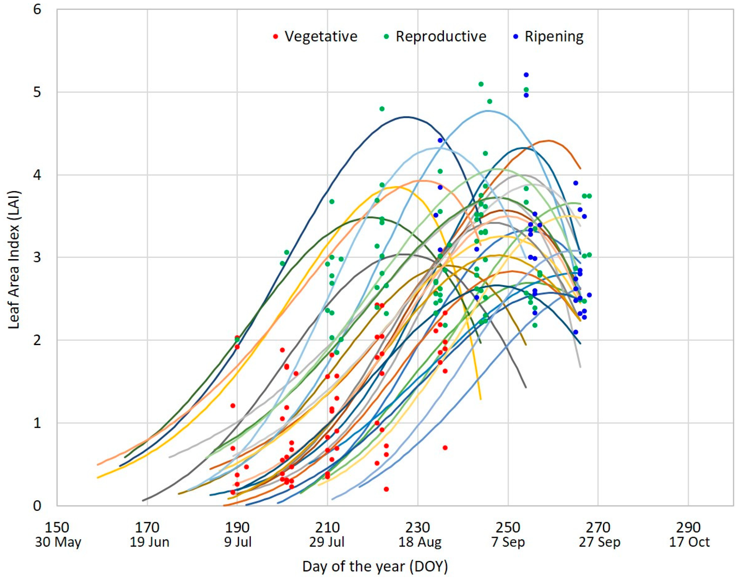
3.1. Interpolated LAI

The use of Baret’s semi mechanistic LAI model filled the missing LAI at the date of image acquisition, allowed the estimation of dates when the heading/flowering stage occurred and removed the noise in the LAI values. The assessment of the accuracy of interpolated LAI against the in situ LAI showed a statistically significant and strong correlation (R² = 0.89 and RMSE = 0.35) (Figure 3). Based on the transplanting dates from farmers’ interviews, transplanting occurred within a two-month period which can also be seen in Figure 4. The earliest transplanting was on 8 June and the latest was on 5 August 2013. The heading–flowering stage (maximum LAI) based on ground observation for the study sites were observed from day of the year (DOY) 221 (9 August 2013) to DOY 268 (25 September 2013). There is a strong correlation in the occurrence of the peak of LAI (i.e., heading–flowering stage) at the simulated and in situ LAI measurements (R² = 0.82 and RMSE = 6 days). The maximum interpolated LAI values for the 30 rice fields ranged from 2.5 to 4.8.

The trend of the interpolated LAI for the whole rice crop cycle is shown in Figure 5. LAI increased continuously from the vegetative phase until it reached the maximum at the end of reproductive phase (heading–flowering stage) (Table S2). As the rice crop entered the ripening phase (milky–dough stage), LAI decreased continuously until the maturity stage.

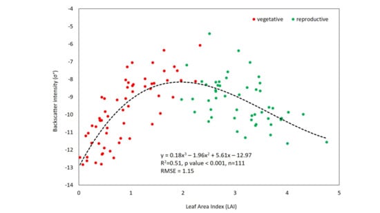
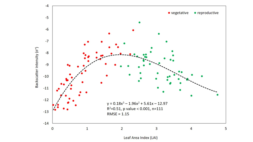
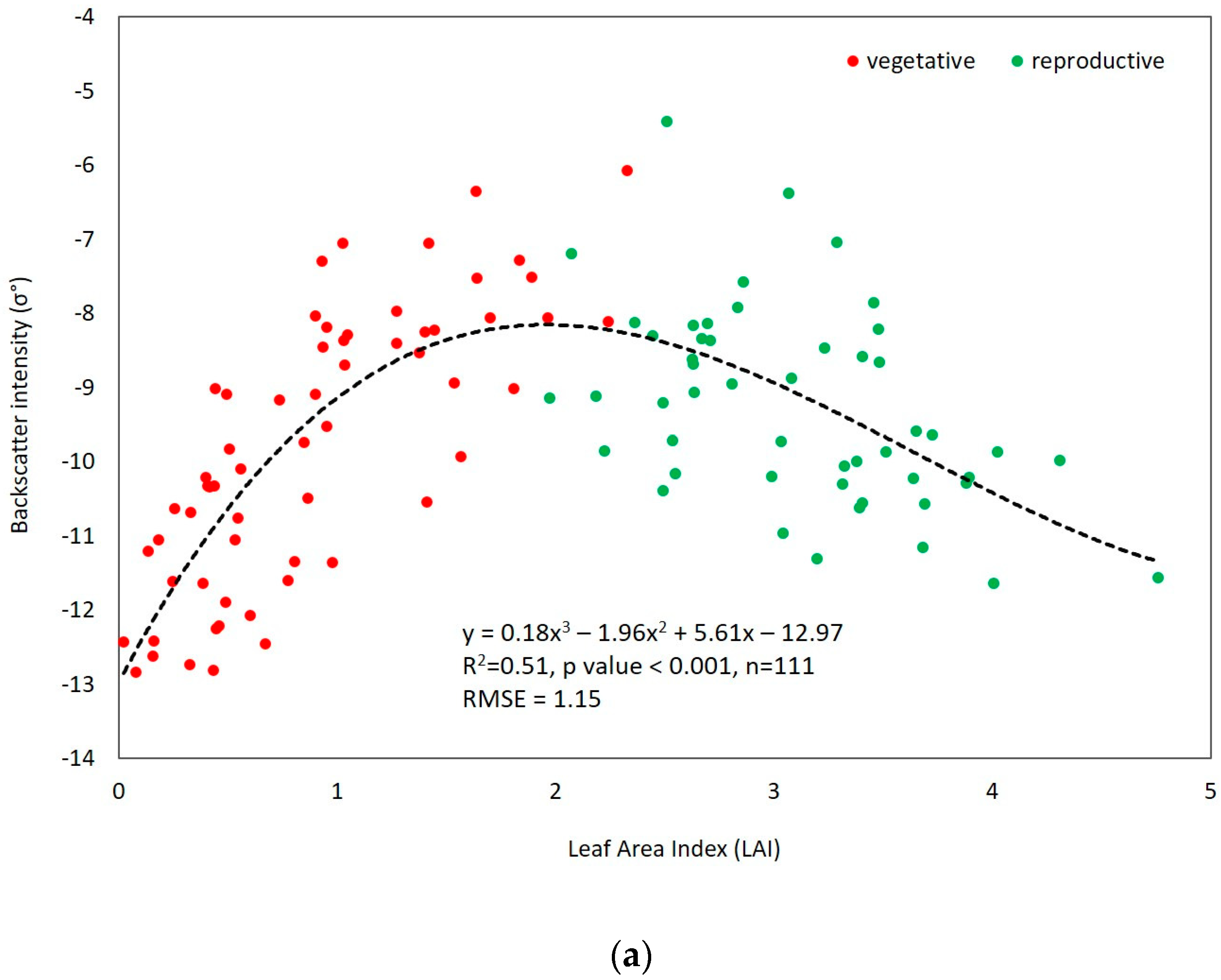
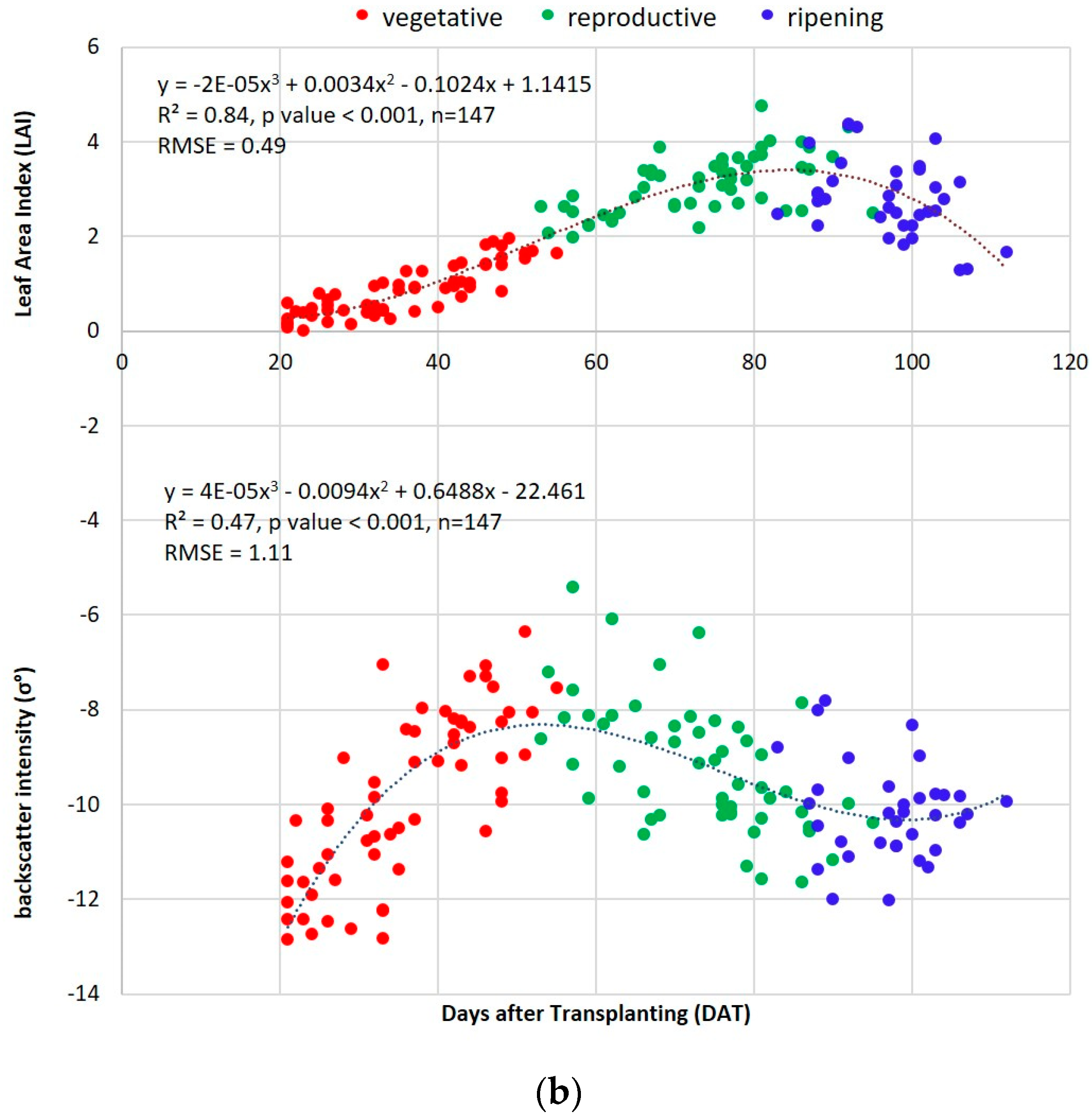
3.2. Relationship Between Backscatter Intensity (σ°) and Interpolated LAI

Figure 6a shows a non-linear trend in the relationship of σ° and LAI from the vegetative to reproductive phases. The use of polynomial regression to approximate the non-linear relationship between σ° and LAI (vegetative to reproductive phase) gave a statistically significant result with R² = 0.51, p value < 0.001 and RMSE = 1.15.

An increasing trend in the relationship of σ° with LAI was found to occur at the vegetative phase (from newly transplanted seedling to the tillering–stem elongation stage), where the average σ° increased from −11.41 dB to −8.59 dB along with the increase in the average LAI from 0.39 to 1.25. At the reproductive phase (panicle initiation to end of the heading–flowering stage), the average σ° ranged from −8.58 dB to −9.64 dB indicative of saturation (Figure 6a). LAI, on the other hand, continued to increase at the reproductive phase from 2.75 to 3.31 as it reached its peak (Figure 6b).

For the ripening phase (milking to maturity stage), there was no significant relationship between LAI and σ°. A non-significant linear trend that is almost horizontal with a slope of −0.19 was detected (R² = 0.02, p value = 0.37 and RMSE = 0.96), approaching an asymptotic relationship. The average σ° at the ripening phase ranged from −10.09 dB to −9.93 dB while the average LAI dropped from 3.05 to 2.20. By the time the last image was acquired on 23 September 2013, 77% of the monitoring fields already reached the ripening phase (milking to maturity stage).

Figure 6b shows a statistically significant and very strong relationship (R² = 0.84, p value < 0.001 and RMSE = 0.49) between days after transplanting (DAT) and LAI, whereas the relationship between σ° and DAT is less strong (R² = 0.47, p value < 0.001 and RMSE = 1.11).

Table 3. Summary of findings from this study and previous studies on the relationship between X-band backscattering intensity (σ°) and rice crop’s LAI.

Frequency Bands	Sensor	Wavelength (cm)	Incident Angle (◦)	Polarisation	Spatial Resolution (m)	Temporal Resolution (days)	Crop Growth Phase Studied	Relationship with LAI	R2	Sample Size	Source
X	TSX (ScanSAR)	3.11	45°	HH	18.5	11	Vegetative to reproductive phase (seedling to flowering stage)	Statistically significant non-linear relationship and moderate correlation	0.51	111	this study
							Ripening phase (milking to maturing stage)	Poor correlation	0.02	36
X	CSK (Spotlight mode)	3.11	54°	VV	1	Single image acquired	Late maturing stage	Poor correlation	0.0064	58	Inoue et. al., 2012 [13]
X	TSX and CSK (Spotlight mode)	3.11	44°, 50°, 55°	VV	1.7 × 1.48, 1x1	Once per season	Transplanting and late maturing stage	Poor correlation	−0.21 (maturing)	not mentioned	Inoue et al, 2014 [23]
X	CSK (ScanSAR Wide Region mode)	3.11	45°	HH	30	16	Before the heading stage	Statistically significant correlation	0.34	30	Hirooka et al. 2015 [24]

summarizes the results from this study and other previous research on the relationship between X-band σ° and LAI at various growth stages and using different sensors and polarisations.

4. Discussion

Relationship between Backscatter Intensity (σ°) and Interpolated LAI

The results from this study showed that there is a statistically significant non-linear relationship between the increasing LAI and σ° at the vegetative to reproductive phases with R² = 0.51 and RMSE = 1.15 (Figure 6a). The 51% variability in σ° can be explained by the LAI, while the remaining 49% could probably be attributed to the effect on σ° of different agronomic factors (e.g., rice variety), crop management (e.g., fertilizers applied and timing) resulting in different plant vigour, and different transplanting dates (that occurred within a two-month period).

Asynchronous transplanting is a result of irregular irrigation water release dates, shortage of manual labour, unavailability of machinery for land preparation and transplanting [43], lack of capital, reduced fallow period between DS and WS crops and increased standing crop duration [44]. The two-month transplanting window resulted in varying crop growth stages, different number of LAI measurements for each growth stage and phase, and varying weather conditions at the time of image acquisition that could influence SAR backscatter, especially during the WS.

At the vegetative phase, LAI continuously increased and gradually reached its peak at the late vegetative stage (tillering/stem elongation). X-band is sensitive enough to detect transplanted seedlings [22]. The rougher surface resulting from the erect and open canopy and flooded soil at vegetative phase contributed to the increase in σ° [13,31].

As the rice crop entered the reproductive phase, the σ° gradually decreased as a result of more homogeneous canopy and low surface roughness from closing canopy that covered the stems and rows which acted as vertical scatterers [22]. LAI at this phase continued to increase until it reached its maximum at the heading/flowering stage. At the reproductive phase, the effect of larger LAI value on σ° was diminished and the slope of regression line became less and less positive. This is shown in Figure 6a.

For the ripening phase (i.e., when LAI continuously decreased until the crop was harvested), LAI was found to have a poor linear relationship with σ° (R² = 0.02, p value = 0.37 and RMSE = 0.96) (Figure 6b) which is also in agreement with Inoue et al.’s findings in a separate study for the late maturing stage (R² = 0.04 or r = 0.21) [23]. The relationship between LAI and σ° at the reproductive and ripening phases is less straightforward due to different scattering mechanisms [45].

Our findings of contrasting relationships between σ° and LAI at vegetative to reproductive phases (significant non-linear) and at ripening phase (no relationship) differed from the poor correlation obtained by Inoue et al. [22] and Kim et al. [20]. The difference is likely due to the different datasets used. Inoue et al. analysed the relationship of LAI and σ° using the entire rice growth duration [22].

Hirooka et al. [24] used a dataset for LAI and SAR images that covered the growth stages between transplanting and heading stage. We, on the other hand, covered the entire vegetative and reproductive phase including the heading and flowering stage. Comparing our results with Hirooka et al [24], both obtained a statistically significant relationship between LAI and σ° (Table 3).

The relationship between LAI and σ° at the ripening phase were consistently low (R² < 0.1) whether HH or VV co-polarisation were used (Table 3) [13,23]. This agrees well with the findings of Lopez-Sanchez et al. [19] that rice responds similarly to all incident angles and co-polarisation (HH or VV) at the final stages of the ripening phase.

In our study, we were able to better characterise the relationship of increasing LAI at vegetative to reproductive phases and decreasing LAI at the ripening phase with X-band σ°, contributing to better knowledge on the use of X-band data for estimating LAI for the whole crop cycle, which is essential for the modelling of crop growth and estimation of yield.

5. Conclusions and Recommendations

This study provided information on the relationship between X-band σ° (HH polarisation and 45° incidence angle) and LAI at all rice crop growth phases (vegetative, reproductive and ripening). In particular, this study added new information that LAI and σ° at the vegetative to reproductive growth phases (when LAI is increasing) has a statistically significant non-linear relationship (Figure 6a). This can help researchers in understanding the dynamic relationship between X-band σ° and LAI for the entire rice growing cycle (vegetative to ripening phase), and thereby further improve rice growth modelling using X-band SAR.

We make several recommendations for future research. Firstly, the relationship of X-band VV polarisation information with LAI at all growth phases should be considered. This would provide further information about the relationship between LAI and X-band σ° information at different polarisations, and determine how the response curve would differ from X-band HH polarisation information during increasing LAI (vegetative to reproductive phases) and decreasing LAI (ripening phase). Secondly, the phase difference of HH and VV is known to be useful for crop identification or crop condition discrimination [11], hence future work on the use of phase difference that highlights different information given by different polarisation for rice mapping or rice biophysical parameter extraction could be explored to increase the accuracy of LAI retrieval from SAR. Finally, our backward approach where we identified statistical relationships between rice LAI and SAR backscatter can be complemented with forward approaches or model inversion approaches to generate plant characteristics from the SAR observations.

References

1. LAI-2200 Plant Canopy Analyzer. Available online: https://www.licor.com/documents/6n3conpja6uj9aq1ruyn (accessed on 12 December 2018).
2. González Sanpedro, M. Optical and Radar Remote Sensing Applied to Agricultural Areas in Europe; Universitat de València: Valencia, Spain, 2008. [Google Scholar]
3. Ulaby, F.; Allen, C.; Eger Iii, G.; Kanemasu, E. Relating the Microwave Backscattering Coefficient to Leaf Area Index. Remote Sens. Environ. 1984, 14, 113–133. [Google Scholar] [CrossRef]
4. Yoshida, S. Fundamentals of Rice Crop Science; IRRI: Los Banos, Philippines, 1981. [Google Scholar]
5. Campos-Taberner, M.; García-Haro, F.J.; Camps-Valls, G.; Grau-Muedra, G.; Nutini, F.; Crema, A.; Boschetti, M. Multitemporal and Multiresolution Leaf Area Index Retrieval for Operational Local Rice Crop Monitoring. Remote Sens. Environ. 2016, 187, 102–118. [Google Scholar] [CrossRef]
6. Hoefsloot, P.; Ines, A.; van Dam, J.; Duveiller, G.; Kayitakiret, F.; Hansen, J. Combining Crop Models and Remote Sensing for Yield Prediction: Concepts, Applications and Challenges for Heterogeneous Smallholder Environments; CGIAR: Montpellier, France, 2012. [Google Scholar]
7. Bouman, B.; Van Keulen, H.; Van Laar, H.; Rabbinge, R. The ‘School of De Wit’crop Growth Simulation Models: A Pedigree and Historical Overview. Agric. Syst. 1996, 52, 171–198. [Google Scholar] [CrossRef]
8. Moulin, S.; Bondeau, A.; Delecolle, R. Combining Agricultural Crop Models and Satellite Observations: From Field to Regional Scales. Int. J. Remote Sens. 1998, 19, 1021–1036. [Google Scholar] [CrossRef]
9. Bouman, B. Crop Modelling and Remote Sensing for Yield Prediction. NJAS Wagening. J. Life Sci. 1995, 43, 143–161. [Google Scholar]
10. Zheng, G.; Moskal, L.M. Retrieving Leaf Area Index (LAI) Using Remote Sensing: Theories, Methods and Sensors. Sensors 2009, 9, 2719–2745. [Google Scholar] [CrossRef] [Green Version]
11. Lopez-Sanchez, J.M.; Cloude, S.R.; Ballester-Berman, J.D. Rice Phenology Monitoring by Means of SAR Polarimetry at X-Band. IEEE Trans. Geosci. Remote Sens. 2012, 50, 2695–2709. [Google Scholar] [CrossRef]
12. Yuzugullu, O.; Erten, E.; Hajnsek, I. Estimation of Rice Crop Height from X-and C-Band Polsar by Metamodel-Based Optimization. IEEE J. Sel. Top. Appl. Earth Obs. Remote Sens. 2017, 10, 194–204. [Google Scholar] [CrossRef]
13. Inoue, Y.; Sakaiya, E. Relationship between X-Band Backscattering Coefficients from High-Resolution Satellite SAR and Biophysical Variables in Paddy Rice. Remote Sens. Lett. 2012, 4, 288–295. [Google Scholar] [CrossRef]
14. Darvishzadeh, R.; Skidmore, A.; Schlerf, M.; Atzberger, C. Inversion of a Radiative Transfer Model for Estimating Vegetation LAI and Chlorophyll in a Heterogeneous Grassland. Remote Sens. Environ. 2008, 112, 2592–2604. [Google Scholar] [CrossRef]
15. Nguyen, T.T.H. Earth Observation for Rice Crop Monitoring and Yield Estimation: Application of Satellite Data and Physically Based Models to the Mekong Delta; Faculty of Geo-information Science and Earth Observation, University of Twente: Enschede, The Netherlands, 2013. [Google Scholar]
16. Inoue, Y.; Sakaiya, E.; Wang, C. Capability of C-Band Backscattering Coefficients from High-Resolution Satellite SAR Sensors to Assess Biophysical Variables in Paddy Rice. Remote Sens. Environ. 2014, 140, 257–266. [Google Scholar] [CrossRef]
17. Lopez-Sanchez, J.M.; Ballester-Berman, J.D. Potentials of Polarimetric SAR Interferometry for Agriculture Monitoring. Radio Sci. 2009, 44, 1–20. [Google Scholar] [CrossRef]
18. Special Features of ASAR. Available online: https://earth.esa.int/handbooks/asar/CNTR1-1-5.html#eph.asar.ug.choos.specfeat.selincang (accessed on 1 April 2019).
19. Lopez-Sanchez, J.M.; Vicente-Guijalba, F.; Ballester-Berman, J.D.; Cloude, S.R. Influence of Incidence Angle on the Coherent Copolar Polarimetric Response of Rice at X-Band. IEEE Geosci. Remote Sens. Lett. 2014, 12, 249–253. [Google Scholar] [CrossRef] [Green Version]
20. Kim, Y.-H.; Hong, S.Y.; Lee, H. Radar Backscattering Measurement of a Paddy Rice Field Using Multi-Frequency (L, C and X) and Full-Polarization. In Proceedings of the Geoscience and Remote Sensing Symposium, Boston, MA, USA, 6–11 July 2008. [Google Scholar]
21. Chen, J.; Lin, H.; Huang, C.; Fang, C. The Relationship between the Leaf Area Index (LAI) of Rice and the C-Band SAR Vertical/Horizontal (VV/HH) Polarization Ratio. Int. J. Remote Sens. 2009, 30, 2149–2154. [Google Scholar] [CrossRef]
22. Inoue, Y.; Kurosu, T.; Maeno, H.; Uratsuka, S.; Kozu, T.; Dabrowska-Zielinska, K.; Qi, J. Season-Long Daily Measurements of Multifrequency (Ka, Ku, X, C, and L) and Full-Polarization Backscatter Signatures over Paddy Rice Field and Their Relationship with Biological Variables. Remote Sens. Environ. 2002, 81, 194–204. [Google Scholar] [CrossRef]
23. Inoue, Y.; Sakaiya, E.; Wang, C. Potential of X-Band Images from High-Resolution Satellite SAR Sensors to Assess Growth and Yield in Paddy Rice. Remote Sens. 2014, 6, 5995–6019. [Google Scholar] [CrossRef] [Green Version]
24. Hirooka, Y.; Homma, K.; Maki, M.; Sekiguchi, K. Applicability of Synthetic Aperture Radar (SAR) to Evaluate Leaf Area Index (LAI) and Its Growth Rate of Rice in Farmers’ Fields in Lao Pdr. Field Crop. Res. 2015, 176, 119–122. [Google Scholar] [CrossRef]
25. De Datta, S.K. Principles and Practices of Rice Production; IRRI: Los Banos, Philippines, 1981. [Google Scholar]
26. Kumar, V.; Kumari, M.; Saha, S.K. Leaf Area Index Estimation of Lowland Rice Using Semi-Empirical Backscattering Model. Appres 2013, 7, 073474. [Google Scholar] [CrossRef]
27. Chen, C.; Quilang, E.; Alosnos, E.; Finnigan, J. Rice Area Mapping, Yield, and Production Forecast for the Province of Nueva Ecija Using Radarsat Imagery. Can. J. Remote Sens. 2011, 37, 1–16. [Google Scholar] [CrossRef]
28. Deparment of Agriculture, Bureau of Soils and Water Management. Land Resources Evaluation Project of Nueva Ecija: The Physical Environment; Deparment of Agriculture, Bureau of Soils and Water Management: Quezon City, Philippines, 2005.
29. Palay and Corn. Area Harvested; Philippine Statictics Authority: Quezon City, Philippines, 2017. Available online: http://openstat.psa.gov.ph/PXWeb/pxweb/en/DB/ DB__2E__CS/0022E4EAHC0.px/?rxid=bdf9d8da-96f1-4100-ae09-18cb3eaeb313 (accessed on 23 February 2017).
30. Climate of the Philippines. Available online: https://www1.pagasa.dost.gov.ph/index.php/climate-of-the-philippines (accessed on 15 August 2018).
31. Asilo, S.; de Bie, K.; Skidmore, A.; Nelson, A.; Barbieri, M.; Maunahan, A. Complementarity of Two Rice Mapping Approaches: Characterizing Strata Mapped by Hypertemporal Modis and Rice Paddy Identification Using Multitemporal SAR. Remote Sens. 2014, 6, 12789–12814. [Google Scholar] [CrossRef]
32. GADM Maps and Data. Version 2.8 Ed. Available online: https://gadm.org/ (accessed on 25 August 2015).
33. Liew, S.C.; Kam, S.P.; Tuong, T.P.; Chen, P.; Minh, V.Q.; Lim, H. Application of Multitemporal Ers-2 Synthetic Aperture Radar in Delineating Rice Cropping Systems in the Mekong River Delta, Vietnam. IEEE Trans. Geosci. Remote Sens. 1998, 36, 1412–1420. [Google Scholar] [CrossRef]
34. Nelson, A.; Setiyono, T.; Rala, A.; Quicho, E.; Raviz, J.; Abonete, P.; Maunahan, A.; Garcia, C.; Bhatti, H.; Villano, L.; et al. Towards an Operational SAR-Based Rice Monitoring System in Asia: Examples from 13 Demonstration Sites across Asia in the Riice Project. Remote Sens. 2014, 6, 10773–10812. [Google Scholar] [CrossRef]
35. SARMAP. MAPscape-RICE. Version 5.064; SARMAP: Cascine de Barico, Switzerland, 2013. [Google Scholar]
36. Daily TRMM and Other Satellites Precipitation Product (3b42 V6 Derived). Available online: https://pmm.nasa.gov/data-access/downloads/trmm (accessed on 10 August 2015).
37. AccuPAR PAR/LAI Ceptometer. Available online: http://manuals.decagon.com/Manuals/10242_Accupar%20LP80_Web.pdf (accessed on 19 April 2018).
38. Maclean, J.; Hardy, B.; Hettel, G. Rice Almanac: Source Book for One of the Most Important Economic Activities on Earth; IRRI: Los Banos, Philippines, 2013. [Google Scholar]
39. Baret, F. Contribution Au Suivi Radiometrique de Cultures de Cereales; Universite de Paris-Sud: Paris, France, 1986. [Google Scholar]
40. Koetz, B.; Baret, F.; Poilvé, H.; Hill, J. Use of Coupled Canopy Structure Dynamic and Radiative Transfer Models to Estimate Biophysical Canopy Characteristics. Remote Sens. Environ. 2005, 95, 115–124. [Google Scholar] [CrossRef]
41. NASA Prediction of Worldwide Energy Ressources: Climatology Resource for Agroclimatology. Available online: https://power.larc.nasa.gov/ (accessed on 16 October 2017).
42. Biostatistics Open Learning Textbook. Available online: http://bolt.mph.ufl.edu/6050-6052/unit-1/case-q-q/scatterplots/ (accessed on 3 January 2018).
43. Loevinsohn, M.E. Asynchrony in Cultivation among Philippine Rice Farmers: Causes and Prospects for Change. Agric. Syst. 1992, 41, 419–439. [Google Scholar] [CrossRef]
44. Loevinsohn, M.E.; Litsinger, J.A.; Bandong, J.P.; Alviola, A.; Kenmore, P. Synchrony of Rice Cultivation and the Dynamics of Pest Populations: Experimentation and Implementation; IRRI: Los Banos, Philippines, 1982; p. 20. [Google Scholar]
45. Bouvet, A.; Le Toan, T.; Dao, N.L. Estimation of Agricultural and Biophysical Paramters of Rice Fields in Vietnam Using X-Band Dual-Polarization SAR. In Proceedings of the 2014 IEEE Geoscience and Remote Sensing Symposium, Quebec City, QC, Canada, 13–18 July 2014. [Google Scholar]
Figure 1. TSX ScanSAR image acquired on 25 May 2013 with 30 monitored sites (red dots) in Nueva Ecija during the WS 2013. The yellow lines are the boundaries of municipalities of Nueva Ecija from the GADM database of Global Administrative Areas [32].
Remotesensing 11 01462 g001
Figure 2. Photos depicting the general appearance of rice crop at different rice crop growth stages during the 2013 wet season (WS).
Remotesensing 11 01462 g002
Figure 3. Linear relationship between in situ and interpolated LAI. The blue dashed line is the 1:1 line.
Remotesensing 11 01462 g003
Figure 4. Interpolated LAI curves of the 30 monitored rice fields using Baret’s semi-mechanistic LAI model overlaid with the in situ LAI measurements at different growth phases (vegetative, reproductive and ripening). The LAI curves cover the DOY period from transplanting to harvesting during the 2013 WS.
Remotesensing 11 01462 g004
Figure 5. The boxplots of the interpolated LAI per growth stage (a) and phase (b) for the 30 monitored sites. The following data are shown in the boxplot: median (horizontal black line in the middle of the box), min and max (extent of dashed lines), the 25th and 75th percentile (upper and lower half of the box) and outlier (black dot).
Remotesensing 11 01462 g005
Figure 6. (a) The relationship of backscatter intensity (σ°) with LAI for the vegetative (seedling–tillering) and reproductive phase (panicle initiation–booting to heading–flowering). The black line is the fitted regression line and each data point is represented by a different colour depicting the growth phase at the time of field observation. (b) The relationship of LAI (top scatter plot) and X-band backscattering coefficient (bottom) with days after transplanting (DAT) that covers transplanting to ripening phase.
Remotesensing 11 01462 g006aRemotesensing 11 01462 g006b