Multiple-Scale Variations of Sea Ice and Ocean Circulation in the Bering Sea Using Remote Sensing Observations and Numerical Modeling

Abstract

The Bering Sea is located between the Aleutian Low and Siberian High, with strong seasonal variations in the oceanic circulation and the sea ice coverage. Within such a large-scale system, the physical processes in the Bering Sea carry interannual variability. The special topography in the Bering Sea traps a strong jet along the Bering Slope, whose instability enriches the eddy activity in the region. A Regional Oceanic Modeling System (ROMS), coupled with a sea ice module, is employed to study multiple-scale variability in the sea ice and oceanic circulation in the Bering Sea for interannual, seasonal, and intra-seasonal eddy variations. The model domain covers the whole Bering Sea and a part of the Chukchi Sea and south of Aleutian Islands, with an averaged spatial resolution of 5 km. The external forcings are momentum, heat, and freshwater flux at the surface and adaptive nudging to reanalysis fields at the boundaries. The oceanic model starts in an equilibrium state from a multiple year cyclical climatology run, and then it is integrated from years 1990 through 2004. The 15 year simulation is analyzed and assessed against the observational data. The model accurately reproduces the seasonal and interannual variations in the sea ice coverage compared with the satellite-observed sea ice data from the National Snow and Ice Data Center (NSIDC). Sea surface temperature and eddy kinetic energy patterns from the ROMS agree with satellite remote sensing data. The transportation through the Bering Strait is also comparable with the estimate of mooring data. The mechanism for seasonal and interannual variation in the Bering Sea is connected to the Siberia-Aleutian index. Eddy variation along the Bering Slope is discussed. The model also simulates polynya generation and evolution around the St. Lawrence Island.

1. Introduction

The Bering Sea is a semi-enclosed sea bounded on the northwest by Siberia, on the west by the Kamchatka Peninsula, on the east by Alaska, and on the south by the Aleutian Islands. The Bering Strait, 85 km in width and 50 m in depth on average, is the only ocean gateway between the Pacific and Arctic Oceans. The prominent feature in the bottom bathymetry in the Bering Sea is the Bering Slope, which runs through the Bering Sea from the west to the east, with a sharp change in the water depth from 200 meters on the northeastern side to 2000 meters on the southwestern side within less than 100 km in width, see Figure 1. The oceanic circulation and other physical and biological processes are also significantly characterized by the presence of the Bering Slope. Due to the interaction between the baroclinic instability and the slope, numerous mesoscale eddies are generated along the Bering Slope [1,2,3,4]. Significant eddy activities along the slope partially contribute to an enhanced biological productivity zone called the “green belt” [5,6,7].

The Bering Sea is located at the interface between the north of the Aleutian Low and the southeast of the Siberian High. A large seasonal variation is observed in the Aleutian Low. In winter, the Aleutian Low is very strong, with a strong northeasterly wind over the Bering Sea, and in summer, the Aleutian Low becomes weak and even disappears, which results in a weak southwesterly wind blowing over the Bering Sea. The northeasterly wind in the winter carries the cold air from the polar area and causes the sea water to freeze and form sea ice. The southwesterly wind in summer brings warm air from the south to the Bering Sea, contributing to the sea ice melting [8]. This large seasonal variation in forcing is reflected in the oceanic circulation field and sea ice distribution [9,10,11]. The interannual change in the local winds causes the sizeable interannual variability of the Bering Strait fluxes in volume, heat, and freshwater, eventually resulting in the interannual variability of the sea ice [12,13]. Therefore, the seasonal variation of sea ice is the dominant phenomenon in the Bering Sea [14,15,16,17].

The variation in the Bering Sea’s circulation is also affected by the large-scale circulation in the Pacific Ocean. South of the Aleutian Islands, the Aleutian Stream flows westward on the northern branch of the subpolar gyre. Some significant parts of the Aleutian Stream leak into the Bering Sea and combine with local circulation [18]. The variation in the intensity of the Aleutian Stream, which carries the warm water, affects the Bering Sea circulation and sea ice variation [9,11,19,20].

Numerous observations of sea-ice coverage and hydrological variables have been conducted in the Bering Sea. The sea ice coverage is determined by means of different microwave radiation bands reflecting from the sea ice and open water, as observed from space-borne microwave radiometers [21]. This data can be traced back to the 1970s and provides information on the sea-ice coverage trend in the Bering Sea [22,23,24]. However, most available hydrological observations, such as the vertical profiles of temperature, salinity, and velocity, are located around seasonal ice-free areas, and there is a lack of observations under the sea ice that prohibits quantitative understanding of sea ice variations due to sea ice thickness and water column depth.

The past decades have witnessed increasing applications of numerical modeling to the study of sea ice and circulation variations in the Bering Sea, such as the studies by Clement et al. [25], Wang et al. [20], and Danielson et al. [9]. This ocean-only model is applied to simulate the oceanic circulation in the Bering Sea during the ice-free summertime [26,27], and cannot be used to investigate the most dominant phenomenon in the Bering Sea, the seasonal variation of the sea ice. Pritchard et al. [28] made the first effort to use an ice-ocean-coupled model, though their model’s resolution was coarse (~50 km). Clement et al. [25] used a ~9 km pan-Arctic coupled ice-ocean model and reproduced the ocean transports and interannual variability of the sea ice cover in the Bering Sea, but their model did not include the effects of tides. Wang et al. [20] developed a ~9 km coupled ice-ocean model (CIOM) based on the Princeton Ocean Model (POM) to investigate the ocean circulation and thermodynamic features in the Bering Sea. Danielson et al. [9] applied a sea ice model coupled with the ROMS implemented by Budgell [29] to study the dominant modes of interannual variability in the thermohaline and ice fields over the Bering Sea shelf. They also compared the model results with the satellites’ remote sensing and in-situ observations to examine the performance of the model. However, this study focused mainly on the vertical structure of tidal currents and the temperature and salinity fields. Our study concentrates more on the sea ice variability, ocean eddy kinetic energy, and mesoscale eddy transport.

Overall, multiple-scale variations can take place in the oceanic circulation and sea ice in the Bering Sea. Seasonal and interannual variations of sea ice in the Bering Sea have significant implications for shifts in marine species composition and ecosystem reorganization in the Bering Sea and adjacent oceanic regions [30,31]. Comprehensive investigations are required to gain a reliable knowledge of the aforementioned variations. In the present study, we employ the sea ice model coupled with a ROMS using a high resolution to investigate these multiple-scale variations in the sea ice and ocean circulation in the Bering Sea. This paper is organized as follows. Section 2 introduces data sources along with data inputs, Section 3 describes model configuration, simulation results are given in Section 4, and Section 5 presents the summary and discussion.

2. Data Sources

The following observational measurements are used in the present study: sea ice concentration, sea surface temperature (SST), eddy kinetic energy (EKE), sea surface wind, and air temperature. Sea ice concentration data were obtained from the 1990–2004 monthly SSM/I-measured (Special Sensor Microwave/Imager) microwave brightness temperature data, downloaded from https://nsidc.org/data/NSIDC-0051/versions/1, which is maintained by the National Snow and Ice Data Center (NSIDC) [32]. The data in the polar stereographic projection are provided with a grid cell size of 25 × 25 km. The grid size in the coordinates used is not exactly 25 km (see https://nsidc.org/data/polar-stereo/tools_geo_pixel.html) but slightly smaller than 25 km. The maximum difference is about 4% and the average difference is 2%. Therefore, on average, the sea-ice area and extent calculated from the SSM/I data is about 8% larger than the true sea-ice area and extent. The data were generated using the NASA Team algorithm, which uses a polarization ratio at 19 GHz and a gradient ratio of 19 V and 37 V. The average accuracy of NASA Team algorithm is within $\pm 5\%$ in winter in a compact ice pack, but it is hard to validate datasets at 0% and 100% because they are not designed to enable retrievals outside a sea ice concentration range of 0%–100% [33].

AVHRR-v2(AVHRR stands for “Advanced Very High Resolution Radiometer data”.) SST data is also used (https://www.ncei.noaa.gov/thredds/catalog/OisstBase/NetCDF/AVHRR/catalog.html). The data has a daily temporal resolution and a 0.25° grid resolution. The EKE was calculated from the AVISO(AVISO stands for “Archiving, Validation and Interpretation of Satellite Oceanographic data”.) altimetry-measured Sea Surface Height Anomaly (SSHA) (downloaded from http://www.aviso.oceanobs.com/duacs/), with a spatial resolution of $1/3°\times 1/3°$ and a 7 day temporal window over the period from January 1993 to December 2004.

Monthly sea surface wind and air temperatures from NCEP (National Center of Environmental Prediction) reanalysis dataset were used to analyze the physical mechanism. The 6 hourly (four times a day: 0000, 0600, 1200, and 1800 UTC) meteorological data from the same data source were used to force the numerical model. All the data were downloaded from https://rda.ucar.edu/datasets/ds093.0/ which has a spatial resolution of 0.3 degree.

3. Model

3.1. ROMS

ROMS solves rotating primitive equations with a realistic equation of state [34]. The model uses a generalized sigma-coordinate system in the vertical direction and a curvilinear grid in the horizontal plane. ROMS is a split–explicit, free-surface oceanic model, in which short time steps are used to advance the surface elevation and barotropic momentum equations, with a larger time step used for temperature, salinity, and baroclinic momentum. A third-order, upstream-biased advection operator allows the generation of steep gradients in the solution, enhancing the effective resolution of the solution for a given grid size when the explicit viscosity is small. The vertical mixing is parameterized using a K-profile parameterization (KPP) scheme [35].

3.2. Sea Ice Model and Processing

A sea ice model coupled with ROMS is implemented with sea ice dynamics a and thermodynamics module [29]. The sea ice dynamics are based on an elastic-viscous-plastic (EVP) rheology from Hunke and Dukowics [36] and Hunke [37]. The sea ice thermodynamics are based on Mellor and Kantha [38] and Häkkinen and Mellor [39], with two ice layers and a single snow layer used to solve the heat conduction equation. The atmospheric heat flux is applied to the ice surface, and the stresses caused by the wind and oceanic currents are incorporated into the sea ice model on the top and bottom of the sea ice, respectively. The salinity flux is imposed onto ROMS when the sea ice is formed or melted. Since the Boussinesq approximation is used in ROMS, which ignores density differences except terms multiplied by acceleration due to gravity, water mass is conserved. Therefore, the water mass change due to sea ice melting and freezing is ignored. The output variables include sea ice concentration (percentage per grid) and ice thickness (grid-cell mean). The monthly means of these variables are calculated based on 5 day averaged outputs by averaging 6 records of 5 day averages.

3.3. Model Configuration

The model domain, covering the whole Bering Sea by extending southward to cover the Aleutian Stream and northward to cover the southern portion of the Chukchi Sea, is plotted in Figure 1. The grids follow the zonal and meridional directions, with a maximum grid size of approximately 7 km on the southern end and 3 km on the northern end. West of Kamchatka Peninsula is considered land and is masked off since it has a neglectable influence on the Bering Sea. At the surface, the model is forced by the 6 hourly NCEP reanalysis product with a spatial resolution of 0.3 degrees [40]. The following meteorological parameters used for the forcing are sea surface wind at 10 meters, net heat flux (shortwave radiation and longwave radiation), cloud coverage (albedo), precipitation, and evaporation. The lateral fluxes along the open boundary are interpolated, as interpreted from the monthly SODA (Simple Oceanic Data Assimilation) product. The restoring data for the lateral open-boundary conditions are from the 1990–2004 monthly SODA global oceanic reanalysis product, with a horizontal resolution of $0.5\times 0.5$ degrees and 40 vertical levels [41,42], downloaded from http://iridl.ldeo.columbia.edu/SOURCES/.CARTON-GIESE/.SODA/.v2p0p2-4/. SODA data are applied to the model grid, including temperature, salinity, currents, and Sea-Surface Height (SSH). The solid boundary around islands and the mainland features no-normal and no-slip conditions implemented through a land-mask algorithm [43].

In addition to the meteorological flux at the sea surface, tidal forcing is applied to the simulation along the open boundaries. The tidal amplitudes and phases in both sea surface heights and the barotropic velocities of eight tidal constituents are obtained from a global inverse barotropic tidal model (TPX06) [44,45], which has a horizontal resolution of $0.25°$. The eight tidal constituents are $M_2$, $K_1$, $O_1$, $S_2$, $N_2$, $P_1$,$K_2$, $Q_1$, ordered by their amplitude in the region, and their definitions refer to the website of https://tidesandcurrents.noaa.gov/glossary. The barotropic transport from the TPX0.6 solution is adjusted based on the ROMS bathymetry because the bathymetry fields from the ROMS and TPX06 are different. To account for the 18.6 year cycle of astronomical tidal-generating potentials, nodal correction is applied to the sea surface height and the barotropic transport of the TPX06 [46,47]. These two procedures proved to be important to achieve an accurate barotropic tidal simulation [46].

The model starts from the state in December of 1990 from the SODA product produced by 1990 NCEP forcing and repeated for five years until the model reaches a quasi-steady state. Then, the model is run for 15 years (1990–2004). The five-day averaged model outputs are analyzed in the present study.

4. Results and Analysis

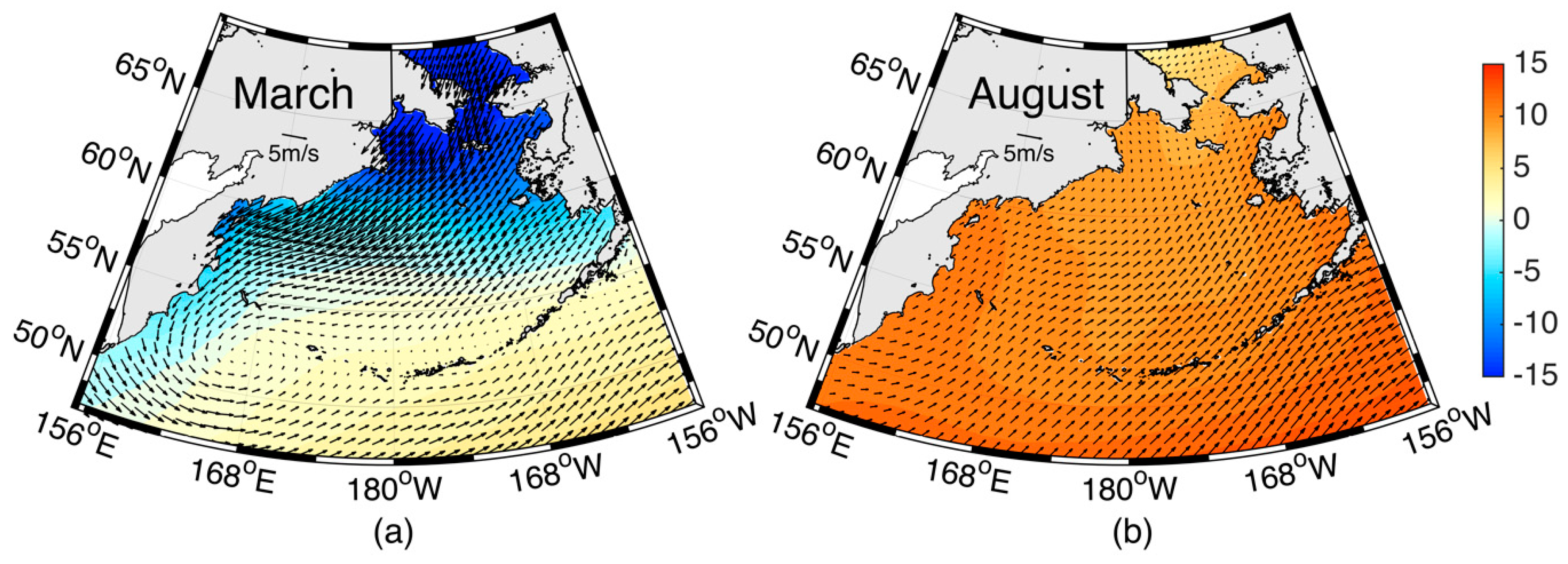
4.1. Seasonal Variation

As introduced in Section 1, the sea ice in the Bering Sea follows a seasonal variation. The Bering Sea is essentially ice free in July through September. Only a few remnants of sea ice are present in June, and sea ice starts to form in October. This can be clearly seen from the remote sensing data of the sea ice.

To calculate the monthly sea-ice area in the Bering Sea from 1990 to 2004, we multiply the sea-ice concentration with the grid cell area at each grid for each month, and then sum all the grid sea-ice areas. The time series of the 15 year averages of monthly sea-ice areas in the Bering Sea for each month are plotted in Figure 2a in a solid line. Dashed lines are the values plus/minus one standard deviation representing its interannual variation. The figure shows that the sea ice area reaches the maximum in March and the minimum in August and illustrates that the sea ice starts to form in late September and early October. The standard deviation (the difference between the dashed lines and solid lines in Figure 2) represents the interannual variation for each month. It can be clearly seen that the interannual variation varies from month to month. In winter and early spring (DJFMA), it is much larger than that in summer and early fall (JASO). ROMS accurately reproduces the seasonal variation in the sea ice coverage shown in the Figure 2b. However, ROMS produces less sea ice than the SSM/I observed during the winter peak because melting processes are delayed during early summer. The ROMS results exhibit a full month delay. Zero sea-ice areas are found in August in ROMS, while they appear as early as July in the observations. The largest differences seem to occur in May and June. Further, the freeze-up is delayed, as shown by the smaller sea-ice area in November and December in ROMS compared to the observations.

To check the spatial distribution of the sea ice coverage in the Bering Sea, the mean distributions of the sea ice concentration in March and August (averaged over the 1990–2004 SSM/I data) are plotted (Figure 3a,b). In March, the sea ice can be found covering most of the northern shelf of the Bering Sea. On the western Bering Sea, a narrow extension is presented along the eastern coast of Siberia and even northern part of the Kamchatka Peninsula. On the eastern Bering Sea, the whole western coast of the Alaska is covered by the sea ice but with a relatively lower concentration than in the western open ocean. In August, the sea ice in the Bering Sea completely disappears. It should be noted that, to maintain consistency, the land masks for both the model and remote sensing observational data (including sea ice, SST, and AVISO SSH data) are the same ones from the model.

The sea ice model coupled into ROMS can reproduce the above seasonal variation in the sea ice concentration in the Bering Sea. Figure 3c,d plots the model-simulated mean sea ice concentration distribution in March and August, also averaged over 1990–2004. The ice edge produced by the model is very close to that from the SSM/I observations in all directions. There are some differences in the concentration values between the model and observations. Figure 3e,f plots the differences between ROMS and SSMI obtained by ROMS minus SSMI. As can be seen, for example, there is a dipole in the difference in March, which tells us that the ROMS produces more sea ice along the western coast in the southern part and less sea ice along the Bering slope. The ROMS model also fails to reproduce high ice concentrations close to the coast towards the Kamchatka Peninsula. The reasons for these differences might be caused by the imperfect numerical models used. Numerical model systems, such ROMS and the sea ice module, are complicate systems, in which many factors could produce errors, such as the inaccuracy of the ROMS numerical schemes, which calculate the physical processes, such as turbulent mixing and sea-ice-ocean interactions. Some differences could be caused by resolution differences in the SSM/I data and the model configuration. To explore the reasons for such discrepancies requires a series of numerical sensitivity experiments, which is beyond the scope of the present paper.

SST data from satellite observations of the ice-free ocean surface are compared with the model solution. Figure 4a–d show the monthly anomalies from ROMS and satellite AVHRR SST data, respectively. The anomalies are calculated by using a 15 year monthly mean SST minus a 15 year yearly mean SST. Both the model and observations show opposite anomalies during spring and summer. In spring, along the Aleutian Islands and the Bering Slope, positive anomalies are seen for both the model and data, but negative anomalies are observed in summer. Along the Kamchatka coast, the anomalies are different from those along the Bering Slope. In spring, negative anomalies are present while positive anomalies occur in summer. Though the spatial distribution pattern of the observed SST is reproduced by the model, there is systematic discrepancy between the modelled results and satellite observational data. Such numerical errors could be caused by the uncertainties of numerical schemes implemented in the ROMS (e.g., air-sea interaction and upper layer mixing schemes), which need be improved in future.

The oceanic circulation in the Bering Sea also has a correspondingly large seasonal variation. Figure 5 displays the surface mean circulations in March and August averaged over 1990–2004. In March, the circulation is characterized by three jets in the Southern Bering Sea. A westward Aleutian stream enters the Bering Sea through gaps among the islands, a strong jet flows northwestward along the Bering Slope, and a current flows southward along the Kamchatka coast. Sea water spreads over the slope and onto the shelf at the north of the Bering slope, where the sea ice is presented during the wintertime. The poleward surface current is very weak across the Bering Strait during the winter. The circulation pattern shows a dramatic change, especially over the shelf north of the Bering Slope, where the sea ice is absent in August. It is also noted that poleward transport in the Bering Strait is observed much more strongly in August than in March.

The monthly poleward transport through the Bering Strait from ROMS is plotted in Figure 6, in which the solid line is the 15 year mean and dashed lines are values plus/minus one standard deviation value displaying the interannual variation. This demonstrates that the water exchange between the Pacific Ocean and the Arctic Ocean occurs mainly as the Pacific water flows into the Arctic Ocean, which is consistent with reports from the literature, such as the studies by Woodgate and Rebecca [48], Aksenov et al. [49], and Watanabe [50]. Figure 6 shows a strong seasonal variation of poleward transport. In spring and summer, the poleward transport peaks. In November through January, its magnitude is much smaller compared to summer. The poleward transport also carries strong interannual variation, as shown in the figure. The interannual variability (denoted by the standard deviation) is smallest for April through July and largest for November through February. It is 2–3 times more likely to have a poleward transport in February, which is as large as the one in May, than to have a poleward transport in May, which is as low as the result in February. From November through January, the poleward transport reversed to be southward from the standard deviations presented in Figure 6.

The seasonal variation in the sea ice coverage, oceanic circulation, and poleward transport can be explained by sea surface wind forcing and air temperature. Figure 7 shows the sea surface wind and air temperatures in March and August, averaged over 15 years from 1990 to 2004. In March, the strong northeasterly wind dominates, which carries cold air (a few degrees below 0 ℃) from the Arctic Ocean to the Bering Sea, causing sea ice formation in its northern part. The mean wind speed magnitude reaches about 10 m/s. This strong wind facilitates a southward spread of sea ice. In August, a mild southwesterly wind (weaker than 3 m/s) blows over the Bering Sea with air temperatures of about 5–10 ℃ [17]. This temperature helps melt the sea ice completely in the Bering Sea. It should be noted that a cyclonic center of the wind is clearly seen southeast of the Kamchatka Peninsula on the wind map in March, located near the Aleutian Low, but the cyclone disappears in August.

It can be understood that sea surface wind and air temperature changes are related to large- scale climate pattern changes (Aleutian Low and Siberian High) and drive the seasonal variation in sea ice and oceanic circulation [51,52].

4.2. Interannual Variation

The standard deviation in Figure 2 is calculated based on 15 year monthly means and represents the interannual variations in the sea-ice area. As can be seen from Figure 2, the interannual variation varies from month to month. To further demonstrate the interannual variation, Figure 8 shows the yearly means of the sea-ice area from both the model (ROMS) and the observations (SSM/I), for 15 years from 1990 to 2004. This figure clearly shows a decreasing trend in the sea-ice area during the 15 years from 1990 to 2004 for both the ROMS run and the satellite data, with about a 15–20 percentage decrease. The yearly time series also shows a 3–5 year oscillation. The decreasing trend in the sea-ice area within the studied 15 years could be related to a decadal oscillation in a Pacific domain scale [53]. It should be noted that there is relatively larger difference between the model and observation during the period from 1998 to 2002 than in other years. This difference could be caused by the uncertainties in the forcing for the model and the observational data.

As discussed in Section 4.1, seasonal variations in the sea ice and the surface oceanic circulation in the Bering Sea are partially driven by changes of the sea surface wind and air temperature. The latter is highly related to the Aleutian Low. What drives the interannual variation? To address this question, the correlations between several variables are determined (Figure 9, Figure 10 and Figure 11), including:

• The sea ice coverage anomaly and sea surface air temperature;
• The poleward transport anomaly across the Bering Strait and the wind intensity anomaly;
• The sea ice coverage anomaly and Siberia-Aleutian Index.

The time series of the domain-averaged air temperature from the NCEP and the sea ice coverage with the seasonal cycle removed are plotted in Figure 9, and the correlation between air temperature and sea ice coverage is −0.66 at the significance level of 95%. This shows the sea ice variation is significantly affected and correlated with more (less) sea ice, which associates with lower (higher) air temperature.

The domain-averaged poleward transport is defined as follows:

$$T_y\left(y,t\right)={{\displaystyle \int }}_0^{Lx}{{\displaystyle \int }}_0^{H}v\left(x,y,z,t\right)dxdz$$

$$T_{total}\left(t\right)=\frac{1}{Ly}{{\displaystyle \int }}_0^{Ly}{T}_y\left(y,t\right)dy$$

where $Lx$ and $Ly$ are the zonal and meridional sizes of the numerical model domain, respectively. $\mathrm{H}$ is the water depth.

Figure 10 displays the time series of the domain-averaged poleward transport variation and poleward wind speed variation. The correlation reaches 0.71 at a significance level of 95%. This high correlation demonstrates that wind forcing is the main driving factor, which is consistent with Yang and Dai [54]. They applied a coupled model to investigate the effect of the ocean surface winds on meridional transport and found that the absence of surface wind causes a remarkable decrease in poleward oceanic transport. The interannual variation in Figure 8 can also be observed in the poleward mass transport across the Bering Strait, shown in Figure 10.

The Siberia-Aleutian Index represents the difference between the mean winter (DJFM) normalized 700 hPa anomalies in two regions, Siberia (55$°$N–70$°$N, 90$°$E–150$°$E) and Alaska/Yukon (60$°$N–70$°$N, 130$°$W–160$°$W). The base period for the index normalization is 1961–2000. The 700 hPa height data were obtained from the NCEP Reanalysis Project (https://rda.ucar.edu/datasets/ds093.0/). The index represents the local wind intensity in the area and is used to describe the variation of the local climate system. Figure 11 plots the time series of the Siberia-Aleutian index and the sea ice coverage variation. Their correlation is 0.68 at a significance level of 95%. The Siberia-Aleutian index represents a large-scale wind pattern that drives sea surface current and ocean mixing. The oceanic current and the upper ocean mixing could cause the SST variation, which directly affects the sea ice variation [55].

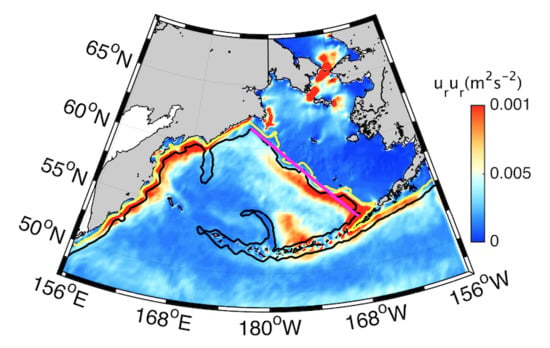
4.3. Intraseasonal (Eddy) Variation

It has been reported in the literature that there are strong eddy activities along the Bering Slope due to the instability of the strong slope current [1,2,3,4]. Five-day averaged model data are used to study the eddy or the intraseasonal variation.

A snapshot of surface vorticity is plotted in Figure 12, showing a well-developed eddy street, which is a repeating pattern of swirling vortices induced by the unsteady separation of the flow along the Bering Slope. The eddies are advected westward by the Bering Slope Current along the slope. Figure 13 plots the EKE calculated from both the ROMS and the AVISO altimetry-measured SSHA data, both of which show an EKE band along the Aleutian Islands, the Bering Slope, the Kamchatka coast, and the Bering Strait. However, the magnitude of the EKE differs between the ROMS and AVISO measurements. This discrepancy is caused by many factors, including the inaccuracy of the model’s numerical schemes, simulating physical processes in the ocean, such as uncertainties in the mixing parameterization, errors in the satellite measurements, the resolution between the ROMS run, and the satellite observations.

Eddy momentum transport across the Bering Slope is plotted in Figure 14b. The seasonal signals larger than 90 days have been high pass filtered. To calculate the eddy transport across the Bering Slope, the coordinates were rotated $\left(90-\mathsf{\theta }\right)$ anticlockwise, where $\mathsf{\theta }$ is the angle between the Bering Slope and the negative direction of the X axis. The velocity components $\mathrm{u}$ and $\mathrm{v}$ are transformed to ${\mathrm{u}}_{\mathrm{r}}$ and ${\mathrm{v}}_{\mathrm{r}}$, where ${\mathrm{u}}_{\mathrm{r}}$ is perpendicular to, and ${\mathrm{v}}_{\mathrm{r}}$ is along, the Bering slope. The magenta straight line approximately follows the 1500 m isobath along the Bering Slope (as shown in Figure 14a). It can be seen that eddy momentum transport is significantly affected by the Bering Slope and mainly located over the Bering Slope. It is also noted that the eddy momentum transports are also large along the Aleutian Islands, the Bering Slope, the Kamchatka coast, and the Bering Strait, which is consistent with the EKE distribution.

4.4. Polynya Evolution

Polynyas are either oceanic areas of open water surrounded by sea ice or areas covered with new or young ice [56]. The St. Lawrence Island polynya is a common phenomenon in the Bering Sea and occurs at least once annually during the winter season [57,58].

As an example, Figure 15 presents the time series of the 5 day averaged sea ice concentration variation around the St. Lawrence Island in April and May, 1996. Polynya evolution can be clearly seen in Figure 15. On 5 April, the polynya begins to form along the southern coastline of the St. Lawrence Island, and increases southwestward when it reaches the maximum extent on 25 April. In May, the polynya forms in the northern coastline of the St. Lawrence Island.

The St. Lawrence Island polynya is formed by the sustained northerly winds in the Bering Sea [57,59], and the St. Lawrence Island polynya is classified as a latent heat polynya with dense water formation south of St. Lawrence Island. Dense water formed during the polynya ice production is the key factor. Therefore, polynyas generate and maintain open-ocean deep convection, which influences thermohaline circulation [57,60,61,62].

5. Summary and Discussion

In this study, the multiple-scale variations of the sea ice area and oceanic circulation in the Bering Sea (intra-seasonal (eddy), seasonal, and interannual) are investigated. Both 15 year (from 1990–2004) satellite remote sensing data and numerical modeling results are employed in the study. This model can reproduce the seasonal and interannual variation in the sea ice area compared with the satellite remote sensing data, including the SST, altimetry-measured SSH, and sea ice. The spatial distribution of the SST and its seasonal variation is exposed by remote sensing data, which is reproduced by a ROMS simulation. The seasonal variation in the sea ice coverage composes the primary variation in the Bering Sea, while the interannual variation is also present, which is revealed by both the model and satellite remote sensing data. Strong intraseasonal variation or events (polynya) can be found around islands via the high-resolution numerical modeling results. The oceanic circulation also has seasonality. A strong vortex street, which separates the shallow part from the deep part in the Bering Sea, is present along the Bering Slope. This sheet can be seen from both the AVISO data and the numerical modeling results.

To explore the mechanisms driving the multiple scale variations in the Bering Sea, the correlations between sea ice coverage and different dynamic parameters, such as the air temperature, SST, sea surface wind, and basin-scale Siberia-Aleutian index are calculated based on both numerical modelling results and observational data. It is revealed that these above variables are important in controlling sea-ice variations in the Bering Sea.

However, there are deviations between the numerical model results from the observational data. These differences could be caused by either uncertainty in the numerical schemes used in the numerical model or observational errors. For examples, there are many empirical parameterizations that need to be improved in both the oceanic numerical model and the sea ice model. The technique used for the remote satellite sensing of sea ice coverage and the algorithm in the calculation of the sea ice need to be improved furthermore. The differences in the model–observation comparison could result from the different resolutions of the two data. Therefore, more effort is needed to improve both the sea-ice ocean coupled model and the observational technique.

References

1. Wang, J.; Ikeda, M. Diagnosing Ocean Unstable Baroclinic Waves and Meanders Using the Quasigeostrophic Equations and Q-Vector Method. J. Phys. Oceanogr. 1997, 27, 1158–1172. [Google Scholar] [CrossRef]
2. Mizobata, K. Variability of Bering Sea eddies and primary productivity along the shelf edge during 1998–2000 using satellite multisensor remote sensing. J. Mar. Syst. 2004, 50, 101–111. [Google Scholar] [CrossRef]
3. Mizobata, K.; Wang, J.; Saitoh, S. Eddy-induced cross-slope exchange maintaining summer high productivity of the Bering Sea shelf break. J. Geophys. Res. Ocean. 2006, 111, C10017. [Google Scholar] [CrossRef]
4. Mizobata, K.; Saitoh, S.; Wang, J. Interannual variability of summer biochemical enhancement in relation to mesoscale eddies at the shelf break in the vicinity of the Pribilof Islands, Bering Sea. Deep Sea Res. Part II Top. Stud. Oceanogr. 2008, 55, 1717–1728. [Google Scholar] [CrossRef]
5. Wang, J.; Hu, H.; Goes, J.; Miksis-Olds, J.; Mouw, C.; D’Sa, E.; Gomes, H.; Wang, D.R.; Mizobata, K.; Saitoh, S.I.; et al. A modeling study of seasonal variations of sea ice and plankton in the Bering and Chukchi Seas during 2007–2008. J. Geophys. Res. Ocean. 2013, 118, 1520–1533. [Google Scholar] [CrossRef]
6. Miller, R.J.; Juska, C.; Hocevar, J. Submarine canyons as coral and sponge habitat on the eastern Bering Sea slope. Glob. Ecol. Conserv. 2015, 4, 85–94. [Google Scholar] [CrossRef] [Green Version]
7. Brown, Z.W.; Arrigo, K.R. Sea ice impacts on spring bloom dynamics and net primary production in the Eastern Bering Sea. J. Geophys. Res. Ocean. 2013, 118, 43–62. [Google Scholar] [CrossRef] [Green Version]
8. Woodgate, R.A.; Weingartner, T.; Lindsay, R. The 2007 Bering Strait oceanic heat flux and anomalous Arctic sea-ice retreat. Geophys. Res. Lett. 2010, 37, 30–31. [Google Scholar] [CrossRef]
9. Danielson, S.; Curchitser, E.; Hedstrom, K.; Weingartner, T.; Stabeno, P. On ocean and sea ice modes of variability in the Bering Sea. J. Geophys. Res. Ocean. 2011, 116, C12034. [Google Scholar] [CrossRef]
10. Frey, K.E.; Moore, G.W.K.; Cooper, L.W.; Grebmeier, J.M. Divergent patterns of recent sea ice cover across the Bering, Chukchi, and Beaufort seas of the Pacific Arctic Region. Prog. Oceanogr. 2015, 136, 32–49. [Google Scholar] [CrossRef]
11. Zhang, J.; Woodgate, R.; Moritz, R. Sea Ice Response to Atmospheric and Oceanic Forcing in the Bering Sea. J. Phys. Oceanogr. 2010, 40, 1729–1747. [Google Scholar] [CrossRef]
12. Woodgate, R.A.; Aagaard, K.; Weingartner, T.J. Interannual changes in the Bering Strait fluxes of volume, heat and freshwater between 1991 and 2004. Geophys. Res. Lett. 2006, 33. [Google Scholar] [CrossRef] [Green Version]
13. Woodgate, R.A.; Weingartner, T.J.; Lindsay, R. Observed increases in Bering Strait oceanic fluxes from the Pacific to the Arctic from 2001 to 2011 and their impacts on the Arctic Ocean water column. Geophys. Res. Lett. 2012, 39, L24603. [Google Scholar] [CrossRef]
14. Niebauer, H.J. Sea ice and temperature variability in the eastern Bering Sea and the relation to atmospheric fluctuations. J. Geophys. Res. Ocean. 1980, 85, 7507–7515. [Google Scholar] [CrossRef]
15. Tateyama, K.; Enomoto, H. Observation of sea-ice thickness fluctuation in the seasonal ice-covered area during 1992−99 winters. Ann. Glaciol. 2001, 33, 449–456. [Google Scholar] [CrossRef]
16. Wang, J.; Ikeda, M. Arctic sea-ice oscillation: Regional and seasonal perspectives. Ann. Glaciol. 2001, 33, 481–492. [Google Scholar] [CrossRef]
17. Li, L.; Miller, A.J.; McClean, J.L.; Eisenman, I.; Hendershott, M.C. Processes driving sea ice variability in the Bering Sea in an eddying ocean/sea ice model: Anomalies from the mean seasonal cycle. Ocean Dyn. 2014, 64, 1693–1717. [Google Scholar] [CrossRef]
18. Stabeno, P.J.; Reed, R.K. Circulation in the Bering Sea Basin Observed by Satellite-Tracked Drifters: 1986–1993. J. Phys. Oceanogr. 1994, 24, 848–854. [Google Scholar] [CrossRef]
19. Okkonen, S.R.; Ashjian, C.J.; Campbell, R.G.; Maslowski, W.; Clement-Kinney, J.L.; Potter, R. Intrusion of warm Bering/Chukchi waters onto the shelf in the western Beaufort Sea. J. Geophys. Res. Ocean. 2009, 114, C00A11. [Google Scholar] [CrossRef]
20. Wang, J.; Hu, H.; Mizobata, K.; Saitoh, S. Seasonal variations of sea ice and ocean circulation in the Bering Sea: A model-data fusion study. J. Geophys. Res. Ocean. 2009, 114. [Google Scholar] [CrossRef]
21. Meier, W.N.; Fetterer, F.; Stewart, J.S.; Helfrich, S. How do sea-ice concentrations from operational data compare with passive microwave estimates? Implications for improved model evaluations and forecasting. Ann. Glaciol. 2015, 56, 332–340. [Google Scholar] [CrossRef] [Green Version]
22. Cavalieri, D.J.; Parkinson, C.L. Arctic sea ice variability and trends, 1979–2010. Cryosphere 2012, 6, 881–889. [Google Scholar] [CrossRef]
23. Parkinson, C.L.; Cavalieri, D.J.; Gloersen, P.; Zwally, H.J.; Comiso, J.C. Arctic sea ice extents, areas, and trends, 1978–1996. J. Geophys. Res. Ocean. 1999, 104, 20837–20856. [Google Scholar] [CrossRef]
24. Parkinson, C.L.; Cavalieri, D.J. A 21 year record of arctic sea-ice extents and their regional, seasonal and monthly variability and trends. Ann. Glaciol. 2017, 34, 441–446. [Google Scholar] [CrossRef]
25. Clement, J.L.; Maslowski, W.; Cooper, L.W.; Grebmeier, J.M.; Walczowski, W. Ocean circulation and exchanges through the northern Bering Sea 1979–2001 model results. Deep Sea Res. Part II Top. Stud. Oceanogr. 2005, 52, 3509–3540. [Google Scholar] [CrossRef]
26. Nihoul, J.C.J.; Adam, P.; Brasseur, P.; Deleersnijder, E.; Djenidi, S.; Haus, J. Three-dimensional general circulation model of the northern Bering Sea’s summer ecohydrodynamics. Cont. Shelf Res. 1993, 13, 509–542. [Google Scholar] [CrossRef]
27. Hermann, A.J.; Stabeno, P.J.; Haidvogel, D.B.; Musgrave, D.L. A regional tidal/subtidal circulation model of the southeastern Bering Sea: Development, sensitivity analyses and hindcasting. Deep Sea Res. Part II Top. Stud. Oceanogr. 2002, 49, 5945–5967. [Google Scholar] [CrossRef]
28. Pritchard, R.S.; Mueller, A.C.; Hanzlick, D.J.; Yang, Y.-S. Forecasting Bering Sea ice edge behavior. J. Geophys. Res. Ocean. 1990, 95, 775–788. [Google Scholar] [CrossRef]
29. Budgell, W.P. Numerical simulation of ice-ocean variability in the Barents Sea region. Ocean Dyn. 2005, 55, 370–387. [Google Scholar] [CrossRef]
30. Grebmeier, J.M. A Major Ecosystem Shift in the Northern Bering Sea. Science 2006, 311, 1461–1464. [Google Scholar] [CrossRef]
31. Grebmeier, J.M. Shifting Patterns of Life in the Pacific Arctic and Sub-Arctic Seas. Annu. Rev. Mar. Sci. 2012, 4, 63–78. [Google Scholar] [CrossRef] [PubMed] [Green Version]
32. Cavalieri, D.J.; Parkinson, C.L.; Gloersen, P.; Zwally, H.J. Updated Yearly. Sea Ice Concentrations from Nimbus-7 SMMR and DMSP SSM/I-SSMIS Passive Microwave Data, Version 1; NASA National Snow and Ice Data Center Distributed Active Archive Center: Boulder, CO, USA, 1996. [Google Scholar]
33. Ivanova, N.; Pedersen, L.T.; Tonboe, R.T.; Kern, S.; Heygster, G.; Lavergne, T.; Sørensen, A.; Saldo, R.; Dybkjær, G.; Brucker, L.; et al. Inter-comparison and evaluation of sea ice algorithms: Towards further identification of challenges and optimal approach using passive microwave observations. Cryosphere 2015, 9, 1797–1817. [Google Scholar] [CrossRef]
34. Shchepetkin, A.F.; McWilliams, J.C. The regional oceanic modeling system (ROMS): A split-explicit, free-surface, topography-following-coordinate oceanic model. Ocean Model. 2005, 9, 347–404. [Google Scholar] [CrossRef]
35. Large, W.G.; McWilliams, J.C.; Doney, S.C. Oceanic vertical mixing: A review and a model with a nonlocal boundary layer parameterization. Rev. Geophys. 1994, 32, 363–403. [Google Scholar] [CrossRef] [Green Version]
36. Hunke, E.C.; Dukowicz, J.K. An Elastic–Viscous–Plastic Model for Sea Ice Dynamics. J. Phys. Oceanogr. 1997, 27, 1849–1867. [Google Scholar] [CrossRef]
37. Hunke, E.C. Viscous–Plastic Sea Ice Dynamics with the EVP Model: Linearization Issues. J. Comput. Phys. 2001, 170, 18–38. [Google Scholar] [CrossRef]
38. Mellor, G.L.; Kantha, L. An ice-ocean coupled model. J. Geophys. Res. Ocean. 1989, 94, 10937–10954. [Google Scholar] [CrossRef]
39. Häkkinen, S.; Mellor, G.L. Modeling the seasonal variability of a coupled Arctic ice-ocean system. J. Geophys. Res. Ocean. 1992, 97, 20285–20304. [Google Scholar] [CrossRef]
40. Kalnay, E.; Kanamitsu, M.; Kistler, R.; Collins, W.; Deaven, D.; Gandin, L.; Iredell, M.; Saha, S.; White, G.; Woollen, J.; et al. The NCEP/NCAR 40-Year Reanalysis Project. Bull. Am. Meteorol. Soc. 1996, 77, 437–471. [Google Scholar] [CrossRef] [Green Version]
41. Carton, J.A.; Chepurin, G.; Cao, X.; Giese, B. A Simple Ocean Data Assimilation Analysis of the Global Upper Ocean 1950–95. Part I: Methodology. J. Phys. Oceanogr. 2000, 30, 294–309. [Google Scholar] [CrossRef]
42. Carton, J.A.; Chepurin, G.; Cao, X. A Simple Ocean Data Assimilation Analysis of the Global Upper Ocean 1950–95. Part II: Results. J. Phys. Oceanogr. 2000, 30, 311–326. [Google Scholar] [CrossRef]
43. Dong, C.; McWilliams, J.C.; Shchepetkin, A.F. Island Wakes in Deep Water. J. Phys. Oceanogr. 2007, 37, 962–981. [Google Scholar] [CrossRef]
44. Egbert, G.D.; Bennett, A.F.; Foreman, M.G.G. TOPEX/POSEIDON tides estimated using a global inverse model. J. Geophys. Res. Ocean. 1994, 99, 24821–24852. [Google Scholar] [CrossRef] [Green Version]
45. Egbert, G.D.; Erofeeva, S.Y. Efficient Inverse Modeling of Barotropic Ocean Tides. J. Atmos. Ocean. Technol. 2002, 19, 183–204. [Google Scholar] [CrossRef] [Green Version]
46. Wang, X.; Chao, Y.; Dong, C.; Farrara, J.; Li, Z.; McWilliams, J.C.; Paduan, J.D.; Rosenfeld, L.K. Modeling tides in Monterey Bay, California. Deep Sea Res. Part II Top. Stud. Oceanogr. 2009, 56, 219–231. [Google Scholar] [CrossRef]
47. Foreman, M.G.G. Manual for Tidal Height Analysis and Prediction; Pacific Marine Science Report 77-10; Institute of Ocean Sciences: Patricia Bay, Sidney, BC, Canada, 1977; 97p. [Google Scholar]
48. Woodgate, R.A.; Rebecca, A. Increases in the Pacific inflow to the Arctic from 1990 to 2015, and insights into seasonal trends and driving mechanisms from year-round Bering Strait mooring data. Prog. Oceanogr. 2018, 160, 124–154. [Google Scholar] [CrossRef] [Green Version]
49. Aksenov, Y.; Karcher, M.; Proshutinsky, A.; Gerdes, R.; De Cuevas, B.; Golubeva, E.; Kauker, F.; Nguyen, A.T.; Platov, G.A.; Wadley, M.; et al. Arctic pathways of pacific water: Arctic ocean model intercomparison experiments. J. Geophys. Res. Ocean. 2016, 121, 27–59. [Google Scholar] [CrossRef]
50. Watanabe, E. Beaufort shelf break eddies and shelf-basin exchange of pacific summer water in the western arctic ocean detected by satellite and modeling analyses. J. Geophys. Res. Ocean. 2011, 116, C08034. [Google Scholar] [CrossRef]
51. Wendler, G.; Chen, L.; Moore, B. Recent sea ice increase and temperature decrease in the Bering Sea area, Alaska. Theor. Appl. Climatol. 2014, 117, 393–398. [Google Scholar] [CrossRef]
52. Rodionov, S.N.; Overland, J.E.; Bond, N.A. The Aleutian Low and Winter Climatic Conditions in the Bering Sea. Part I: Classification. J. Clim. 2005, 18, 160–177. [Google Scholar] [CrossRef]
53. Yu, L.; Zhong, S.; Winkler, J.A.; Zhou, M.; Lenschow, D.H.; Li, B.; Wang, X.; Yang, Q. Possible connections of the opposite trends in Arctic and Antarctic sea-ice cover. Sci. Rep. 2017, 7, 45804. [Google Scholar] [CrossRef] [Green Version]
54. Yang, H.; Dai, H. Effect of wind forcing on the meridional heat transport in a coupled climate model: Equilibrium response. Clim. Dyn. 2015, 45, 1451–1470. [Google Scholar] [CrossRef]
55. Seckel, G.R. First Pacific Symposium on Marine Sciences. Indices for Mid-Latitude North Pacific Winter Wind Systems; an Exploratory Investigation. GeoJournal 1988, 16, 97–111. [Google Scholar] [CrossRef]
56. World Meteorological Organization. WMO Sea Ice Nomenclature; WMO Rep. 259; WMO: Geneva, Switzerland, 1970; 147p. [Google Scholar]
57. Lynch, A.H.; Glueck, M.F.; Chapman, W.L.; Bailey, D.A.; Walsh, J.E. Satellite observation and climate system model simulation of the St. Lawrence Island polynya. Tellus A Dyn. Meteorol. Oceanogr. 1997, 49, 277–297. [Google Scholar] [CrossRef]
58. Drucker, R. Observations of ice thickness and frazil ice in the St. Lawrence Island polynya from satellite imagery, upward looking sonar, and salinity/temperature moorings. J. Geophys. Res. Ocean. 2003, 108, C53149. [Google Scholar] [CrossRef]
59. Schumacher, J.D.; Aagaard, K.; Pease, C.H.; Tripp, R.B. Effects of a shelf polynya on flow and water properties in the northern Bering Sea. J. Geophys. Res. Ocean. 1983, 88, 2723–2732. [Google Scholar] [CrossRef]
60. Killworth, P.D. Deep convection in the World Ocean. Rev. Geophys. 1983, 21, 1–26. [Google Scholar] [CrossRef]
61. Cheon, W.G.; Park, Y.-G.; Toggweiler, J.R.; Lee, S.-K. The Relationship of Weddell Polynya and Open-Ocean Deep Convection to the Southern Hemisphere Westerlies. J. Phys. Oceanogr. 2014, 44, 694–713. [Google Scholar] [CrossRef] [Green Version]
62. Ohshima, K.I.; Nihashi, S.; Iwamoto, K. Global view of sea-ice production in polynyas and its linkage to dense/bottom water formation. Geosci. Lett. 2016, 3, 13. [Google Scholar] [CrossRef]
Figure 1. The numerical model domain. The contours are water depths of 200 m, 1000 m, and 3000 m, respectively.
Remotesensing 11 01484 g001
Figure 2. Seasonal variation in the sea ice covered area in the Bering Sea derived from sea-ice area concentration: (a) from Special Sensor Microwave/Imager (SSM/I) data with the resolution of 25 km; (b) from the regional oceanic modeling system (ROMS) model output data. The solid line is the monthly averaged sea-ice area for 15 years (1990–2004), and the dashed lines are the averages plus/minus one standard deviation.
Remotesensing 11 01484 g002
Figure 3. Seasonal variation in the sea ice coverage percentage in the Bering Sea averaged over 15 years (1990–2004): (a) March and (b) August are derived from the SSM/I data; (c) March and (d) August are derived from the ROMS results. The differences (ROMS minus SSMI) between ROMS and SSM/I are presented for (e) March and (f) August. The model resolution is about 5 km (averaged) and the SSM/I resolution is 25 km.
Remotesensing 11 01484 g003
Figure 4. Seasonal variation in the SST in the Bering Sea: (a) March and (b) August, derived from the ROMS solution; (c) March and (d) August, derived from the AVHRR data. Also shown are the differences (ROMS minus OISST(OISST stands for “Optimum Interpolation Sea Surface Temperature data”.)) between ROMS and OISST for (e) March and (f) August. The monthly mean is averaged over 15 years from 1990–2004 (Unit: K).
Remotesensing 11 01484 g004
Figure 5. Seasonal variation in the surface mean circulations in the Bering Sea: (a) March and (b) August, which are from the ROMS solution averaged over 15 years from 1990–2004. The vector and shading represent the direction and the speed of the current, respectively (Unit: m/s). Vectors are plotted every 8 grid points.
Remotesensing 11 01484 g005
Figure 6. Seasonal variation of the poleward transport through the Bering Strait from the numerical model averaged over 15 years (1990–2004). In oceanography, a Sverdrup is a non-SI (SI stands for “International System of Units”) unit of flow to measure the volumetric rate of the transport of ocean currents, with 1 Sverdrup equal to 1,000,000 m3/s.
Remotesensing 11 01484 g006
Figure 7. Seasonal variation in the air temperature ( Unit :   ) and wind at the sea surface in the Bering Sea: (a) March and (b) August, which are from the National Center of Environmental Prediction (NCEP) reanalysis product and averaged over 15 years (1990–2004).
Remotesensing 11 01484 g007
Figure 8. Interannual variation in the winter-time sea-ice areas in the Bering Sea (unit: km2). The thicker solid and dashed lines are the SSM/I data and the ROMS solution, respectively. The thin solid and dashed lines are from the second order polynomial regression of the SSM/I and ROMS data, respectively. The data are yearly means. Due to the effect of polar stereographic projection, the true SSM/I sea-ice area is possibly smaller than the area shown.
Remotesensing 11 01484 g008
Figure 9. Correlation between the time series of annual sea ice covered area anomaly (solid line, unit: km2) and sea surface air temperature (dashed line, unit: ℃). The sea ice data are from the ROMS solution, and the air temperature data from the NCEP. The sea-ice area anomalies are the yearly mean average minus the 15 year average.
Remotesensing 11 01484 g009
Figure 10. Correlation between the time series of the annual poleward transport anomaly (solid line, unit: Sverdrup) and poleward wind speed anomaly (dashed line, unit: m/s). The poleward transport data are from the ROMS solution and the poleward wind data are from the NCEP.
Remotesensing 11 01484 g010
Figure 11. Correlation between the time series of the annual normalized ice-covered area anomaly (solid line) and Siberia-Aleutian index (dashed line). The sea ice data are from the ROMS solution and the Siberia-Aleutian index is from the NCEP.
Remotesensing 11 01484 g011
Figure 12. Snapshot on April 20th, 1994 of the surface eddy street along the Bering Slope from the 5 day averaged model data. The color is the relative vorticity normalized by the local Coriolis coefficient. The vector denotes the surface current. Contours denote the water depths of 200 m, 500 m, 1000 m, and 2000 m, respectively, as shown in Figure 1.
Remotesensing 11 01484 g012
Figure 13. Mean eddy kinetic energy (EKE) (unit: m2/s2) comparison between (a) the ROMS solution and (b) the AVISO data. The AVISO velocities are derived from gridded satellite altimetry-measured sea surface height-derived data, with the spatial resolution as 1/3 degree. EKE is calculated based on 12 year data (1993–2004). Contours denote water depths of 200 m, 500 m, 1000 m, and 2000 m. On the right panel, the white area in the ocean area is a sea ice covered area with no observations during the winter time, and the AVISO does not provide data for the area.
Remotesensing 11 01484 g013
Figure 14. Eddy transport: (a) schematic diagram of the method and (b) eddy transport across the Bering Slope, which is calculated from the 5 day averaged 15 year data (1990–2004) model data (Unit: m2s−2). The black and yellow lines represent the 1500 m isobath and 200 m isobath, respectively. The straight magenta line is approximately 1500 m of isobaths, which represents the Bering Slope.
Remotesensing 11 01484 g014
Figure 15. Temporal variation of the sea ice concentration (percentage per grid) around the St. Lawrence Island from April 5th to May 10th in 1996 (color represent the averaged fraction of cell covered by the sea ice, red denotes a large fraction and blue denotes a small fraction).
Remotesensing 11 01484 g015