High-Resolution Vegetation Mapping Using eXtreme Gradient Boosting Based on Extensive Features

Abstract
:1. Introduction
2. Materials and Methods
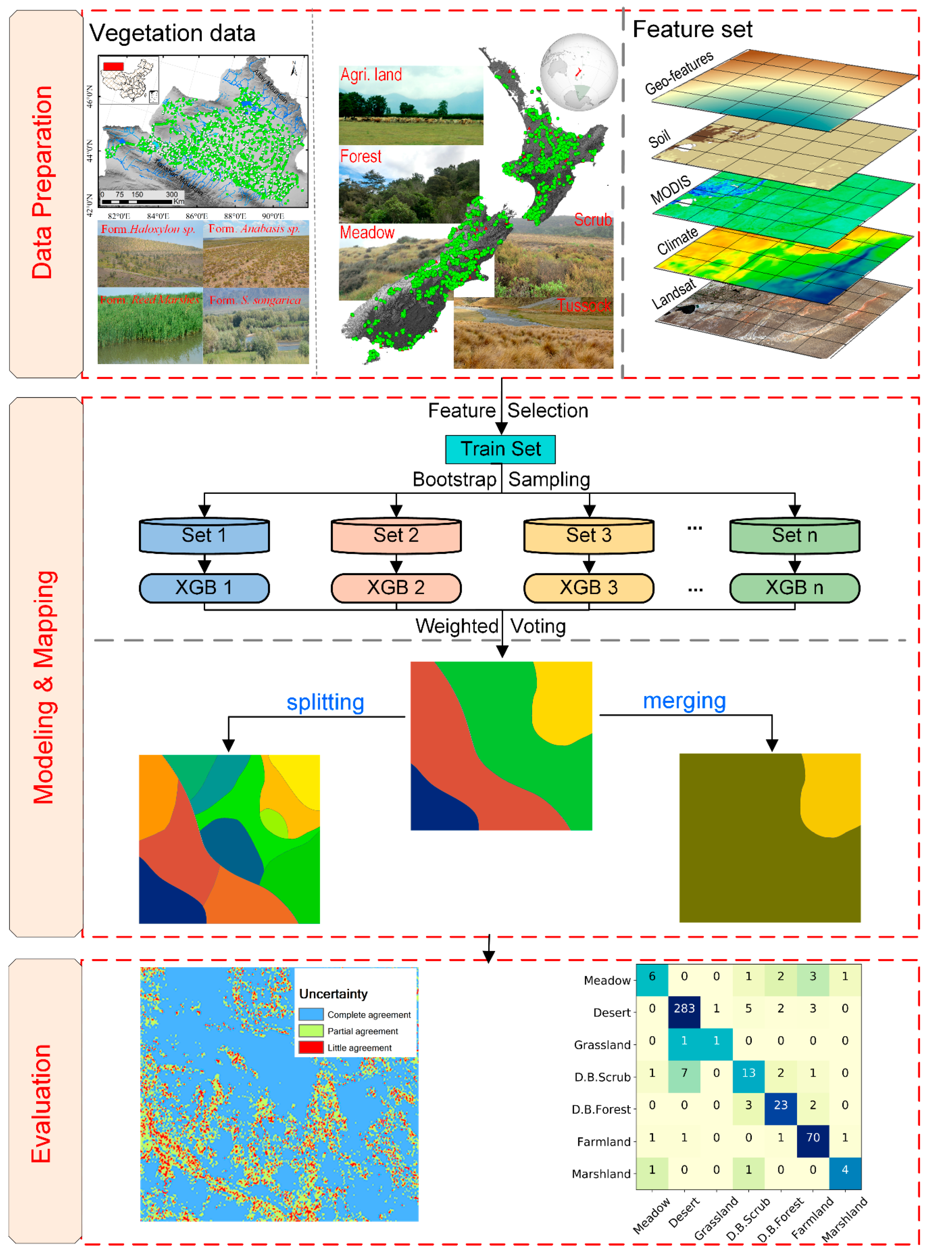
2.1. Data Preparation
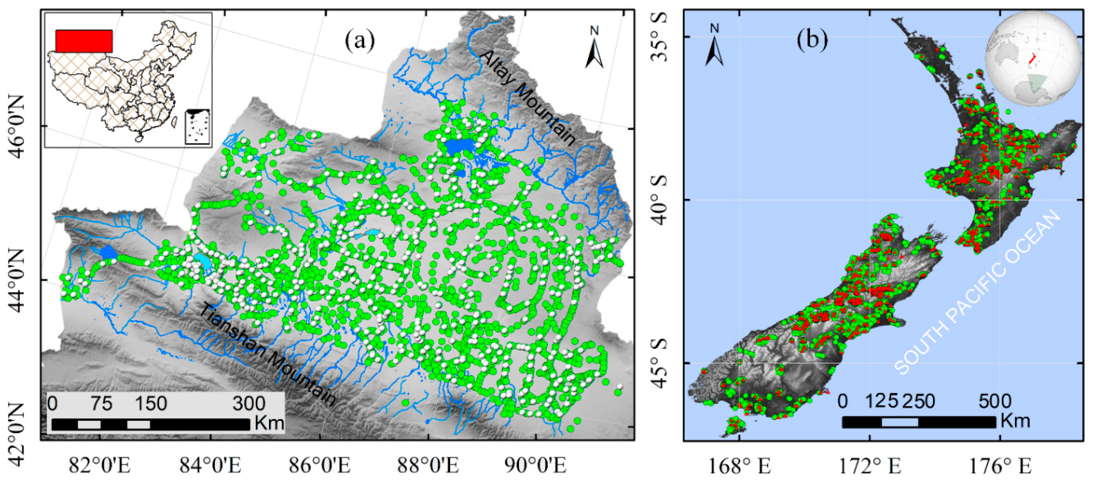
2.1.1. Vegetation Data
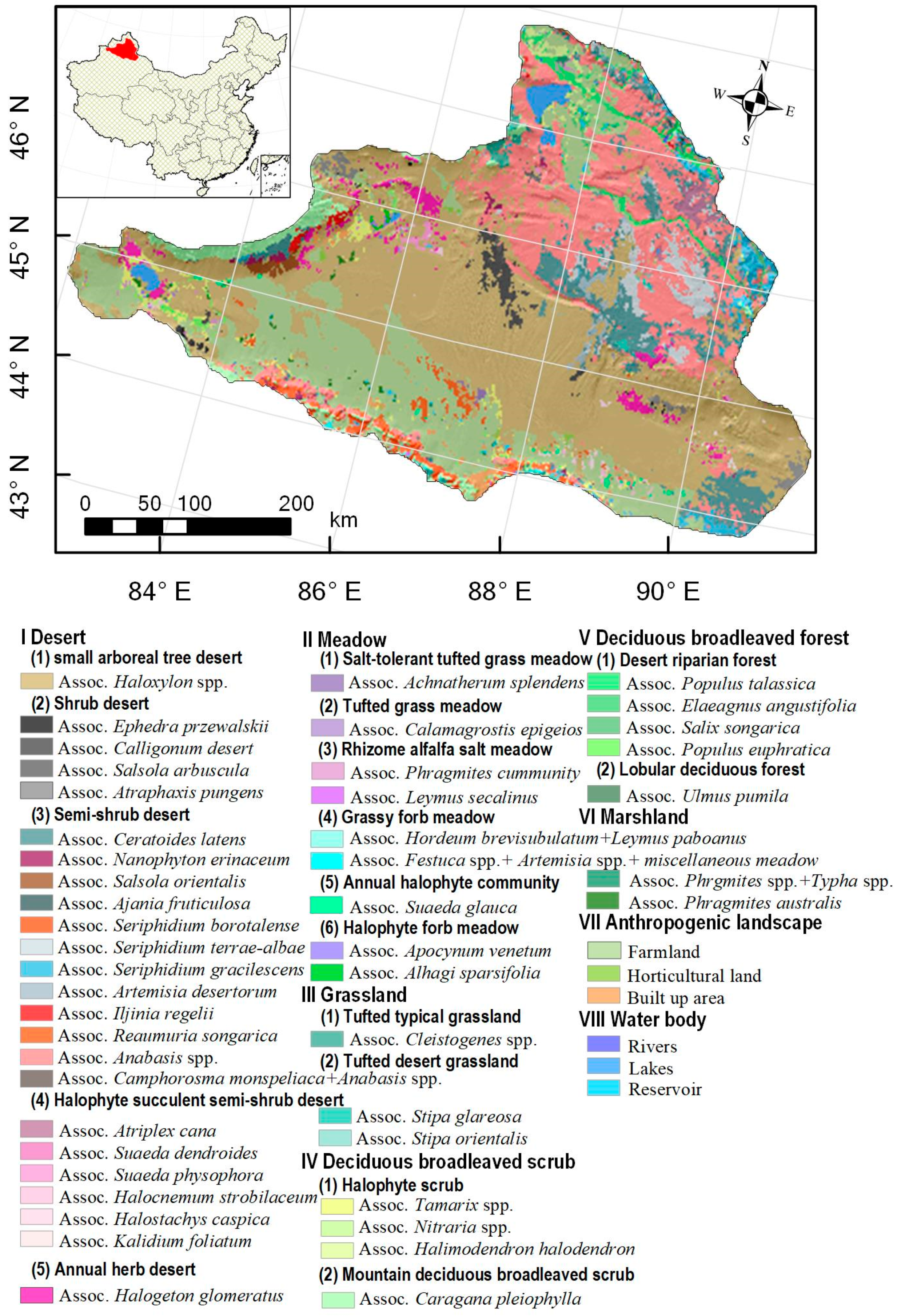
DzB: Simplified Field Survey Data
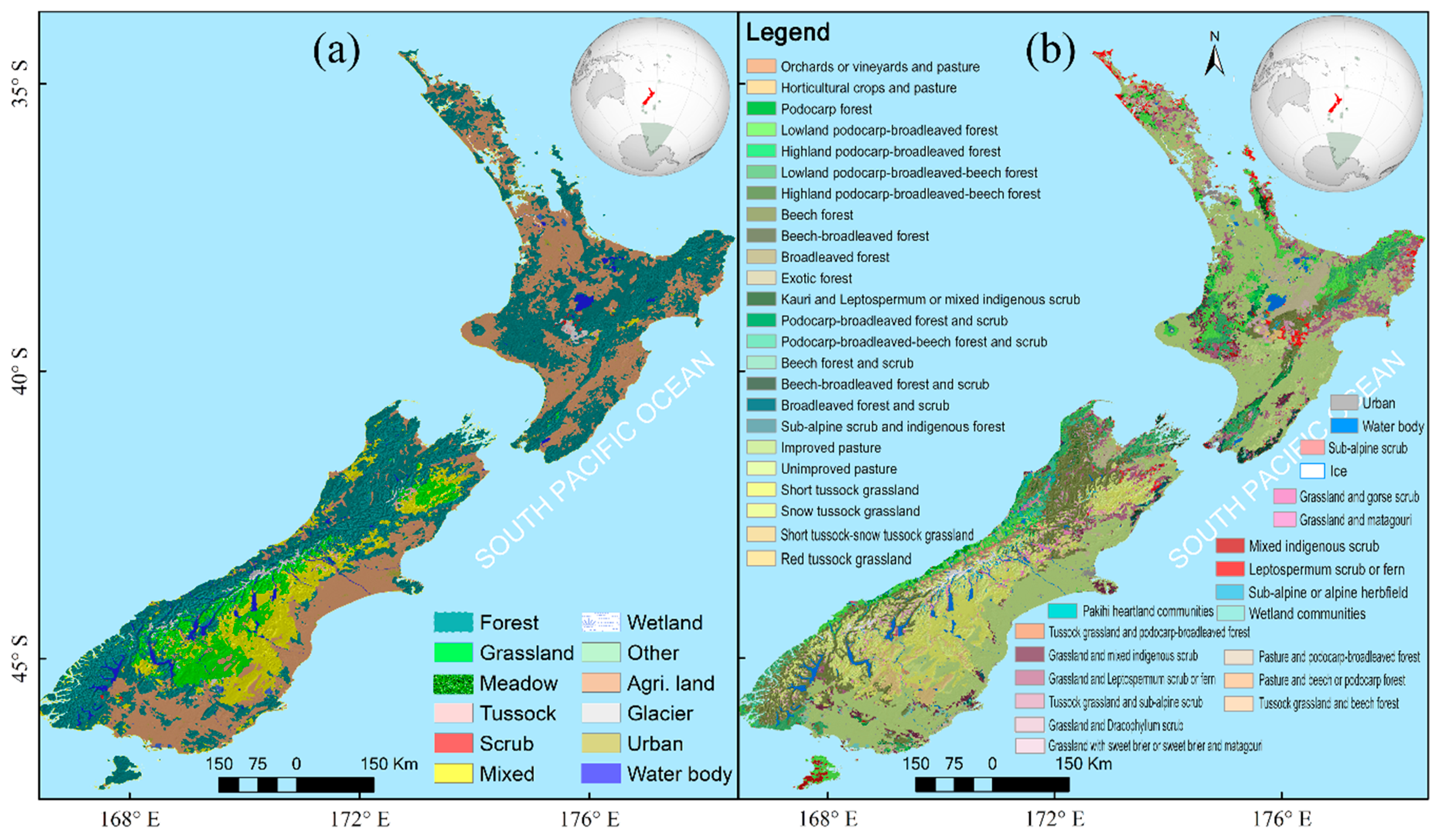
NZ: Simulated Survey Data
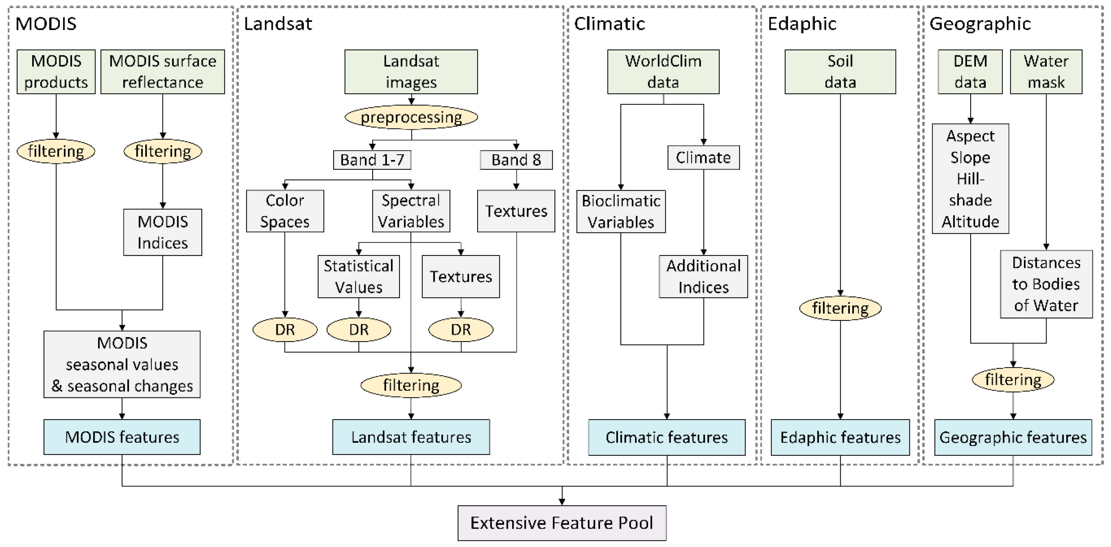
2.1.2. Features
RS Data
Ancillary Data
2.2. Modeling and Mapping
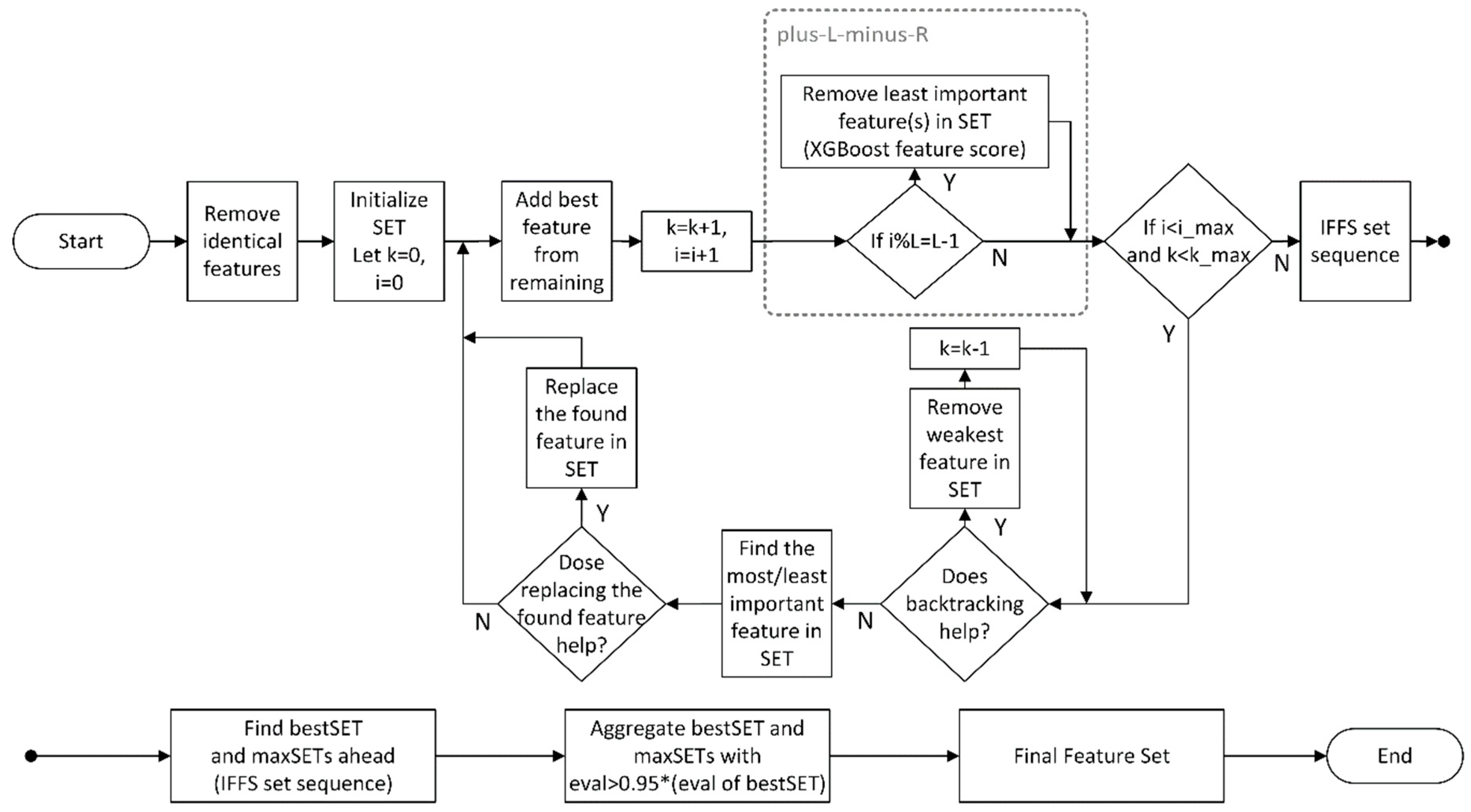
2.2.1. Feature Selection
2.2.2. Vegetation Mapping
2.3. Evaluations
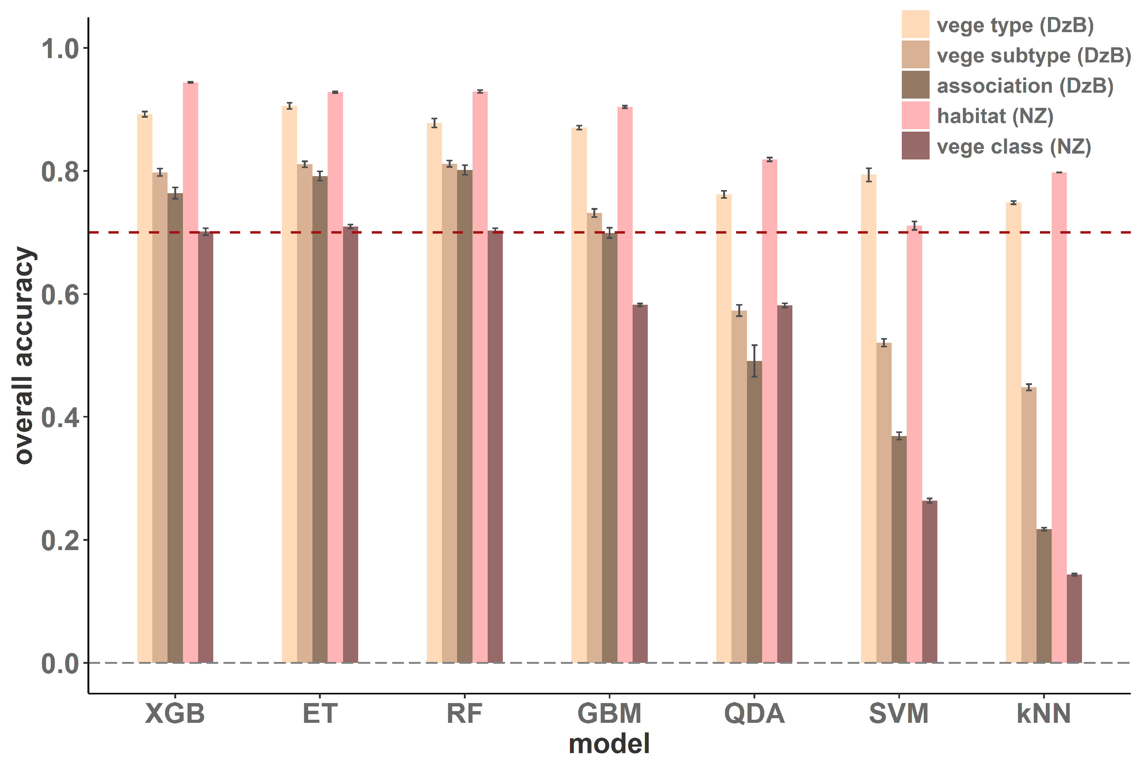
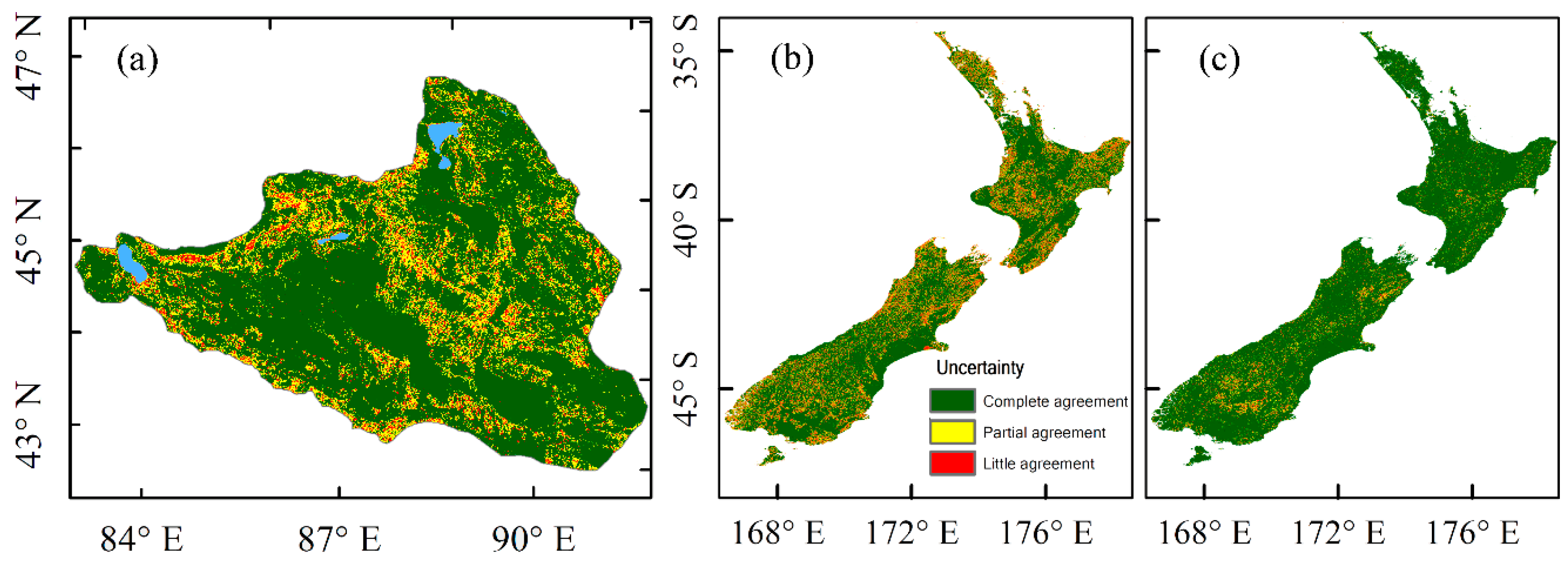
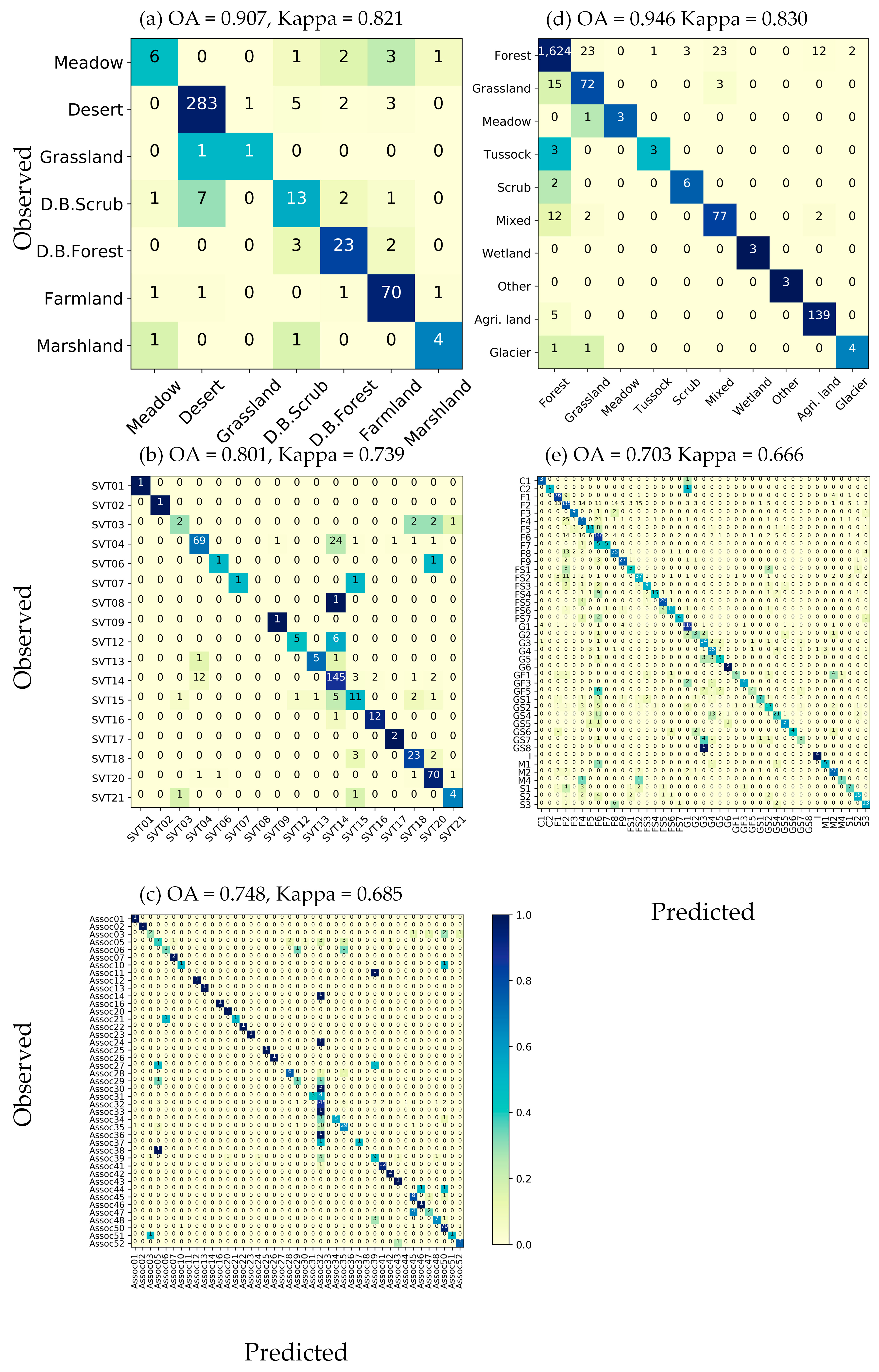
3. Results
4. Discussion
5. Conclusions
Supplementary Materials
Author Contributions
Funding
Acknowledgments
Conflicts of Interest
Appendix A


References
- Assessment, M.E. Millennium ecosystem assessment. In Ecosystems and Human Well-Being: Biodiversity Synthesis; World Resources Institute: Washington, DC, USA, 2005. [Google Scholar]
- Diaz, S.; Pascual, U.; Stenseke, M.; Martin-Lopez, B.; Watson, R.T.; Molnar, Z.; Hill, R.; Chan, K.M.A.; Baste, I.A.; Brauman, K.A.; et al. Assessing nature’s contributions to people. Science 2018, 359, 270–272. [Google Scholar] [CrossRef] [PubMed]
- Pereira, H.M.; Ferrier, S.; Walters, M.; Geller, G.N.; Jongman, R.H.G.; Scholes, R.J.; Bruford, M.W.; Brummitt, N.; Butchart, S.H.M.; Cardoso, A.C.; et al. Essential Biodiversity Variables. Science 2013, 339, 277–278. [Google Scholar] [CrossRef] [PubMed] [Green Version]
- Wang, C.Y.; Guo, Z.Z.; Wang, S.T.; Wang, L.P.; Ma, C. Improving Hyperspectral Image Classification Method for Fine Land Use Assessment Application Using Semisupervised Machine Learning. J. Spectrosc. 2015, 2015, 969185. [Google Scholar] [CrossRef]
- Forzieri, G.; Alkama, R.; Miralles, D.G.; Cescatti, A. Satellites reveal contrasting responses of regional climate to the widespread greening of Earth. Science 2017, 356, 1140–1144. [Google Scholar] [CrossRef] [PubMed]
- Staver, A.C.; Archibald, S.; Levin, S.A. The Global Extent and Determinants of Savanna and Forest as Alternative Biome States. Science 2011, 334, 230–232. [Google Scholar] [CrossRef] [PubMed] [Green Version]
- Küchler, A.W. Vegetation Mapping; Ronald Press Co.: New York, NY, USA, 1967; pp. 853–855. [Google Scholar]
- Malatesta, L.; Attorre, F.; Altobelli, A.; Adeeb, A.; De Sanctis, M.; Taleb, N.M.; Scholte, P.T.; Vitale, M. Vegetation mapping from high-resolution satellite images in the heterogeneous arid environments of Socotra Island (Yemen). J. Appl. Remote Sens. 2013, 7, 073527. [Google Scholar] [CrossRef]
- Pettorelli, N.; Laurance, W.F.; O’Brien, T.G.; Wegmann, M.; Nagendra, H.; Turner, W. Satellite remote sensing for applied ecologists: Opportunities and challenges. J. Appl. Ecol. 2014, 51, 839–848. [Google Scholar] [CrossRef]
- Defourny, P.; Kirches, G.; Brockmann, C.; Boettcher, M.; Peters, M.; Bontemps, S.; Lamarche, C.; Schlerf, M.; Santoro, M. Land Cover CCI. Product User Guide Version 2. Available online: http://maps.elie.ucl.ac.be/CCI/viewer/download.php (accessed on 25 June 2019).
- Giri, C.; Zhu, Z.; Reed, B. A comparative analysis of the Global Land Cover 2000 and MODIS land cover data sets. Remote Sens. Environ. 2005, 94, 123–132. [Google Scholar] [CrossRef]
- Naghibi, S.A.; Pourghasemi, H.R.; Dixon, B. GIS-based groundwater potential mapping using boosted regression tree, classification and regression tree, and random forest machine learning models in Iran. Environ. Monit. Assess. 2016, 188, 44. [Google Scholar] [CrossRef]
- Franklin, J. Predictive vegetation mapping: Geographic modelling of biospatial patterns in relation to environmental gradients. Prog. Phys. Geogr. 1995, 19, 474–499. [Google Scholar] [CrossRef]
- Gorelick, N.; Hancher, M.; Dixon, M.; Ilyushchenko, S.; Thau, D.; Moore, R. Google Earth Engine: Planetary-scale geospatial analysis for everyone. Remote Sens. Environ. 2017, 202, 18–27. [Google Scholar] [CrossRef]
- Jordan, M.I.; Mitchell, T.M. Machine learning: Trends, perspectives, and prospects. Science 2015, 349, 255–260. [Google Scholar] [CrossRef] [PubMed]
- Breckling, B.; Dong, Q. Uncertainty in Ecology and Ecological Modelling. In Handbook of Ecosystem Theories and Management; CRC Press: Boca Raton, FL, USA, 2000; p. 51. [Google Scholar]
- Zhang, C.Y.; Selch, D.; Cooper, H. A Framework to Combine Three Remotely Sensed Data Sources for Vegetation Mapping in the Central Florida Everglades. Wetlands 2016, 36, 201–213. [Google Scholar] [CrossRef]
- Su, L.H. Optimizing support vector machine learning for semi-arid vegetation mapping by using clustering analysis. ISPRS J. Photogramm. Remote Sens. 2009, 64, 407–413. [Google Scholar] [CrossRef]
- Zhang, C.Y.; Xie, Z.X. Object-based Vegetation Mapping in the Kissimmee River Watershed Using HyMap Data and Machine Learning Techniques. Wetlands 2013, 33, 233–244. [Google Scholar] [CrossRef]
- De Colstoun, E.C.B.; Story, M.H.; Thompson, C.; Commisso, K.; Smith, T.G.; Irons, J.R. National Park vegetation mapping using multitemporal Landsat 7 data and a decision tree classifier. Remote Sens. Environ. 2003, 85, 316–327. [Google Scholar] [CrossRef]
- Chen, T.; Guestrin, C. Xgboost: A scalable tree boosting system. In Proceedings of the 22nd ACM Sigkdd International Conference on Knowledge Discovery and Data Mining, San Francisco, CA, USA, 13–17 August 2016; pp. 785–794. [Google Scholar]
- Mitchell, R.; Frank, E. Accelerating the XGBoost algorithm using GPU computing. PeerJ Comput. Sci. 2017, 3, e127. [Google Scholar] [CrossRef]
- Dong, H.; Xu, X.; Wang, L.; Pu, F. Gaofen-3 PolSAR Image Classification via XGBoost and Polarimetric Spatial Information. Sensors 2018, 18, 611. [Google Scholar] [CrossRef]
- Sandino, J.; Pegg, G.; Gonzalez, F.; Smith, G. Aerial Mapping of Forests Affected by Pathogens Using UAVs, Hyperspectral Sensors, and Artificial Intelligence. Sensors 2018, 18, 944. [Google Scholar] [CrossRef]
- Man, C.D.; Nguyen, T.T.; Bui, H.Q.; Lasko, K.; Nguyen, T.N.T. Improvement of land-cover classification over frequently cloud-covered areas using Landsat 8 time-series composites and an ensemble of supervised classifiers. Int. J. Remote Sens. 2018, 39, 1243–1255. [Google Scholar] [CrossRef]
- Zhong, L.H.; Hu, L.N.; Zhou, H. Deep learning based multi-temporal crop classification. Remote Sens. Environ. 2019, 221, 430–443. [Google Scholar] [CrossRef]
- Hirayama, H.; Sharma, R.C.; Tomita, M.; Hara, K. Evaluating multiple classifier system for the reduction of salt-and-pepper noise in the classification of very-high-resolution satellite images. Int. J. Remote Sens. 2019, 40, 2542–2557. [Google Scholar] [CrossRef]
- Jiang, H.; Li, D.; Jing, W.L.; Xu, J.H.; Huang, J.X.; Yang, J.; Chen, S.S. Early Season Mapping of Sugarcane by Applying Machine Learning Algorithms to Sentinel-1A/2 Time Series Data: A Case Study in Zhanjiang City, China. Remote Sens. 2019, 11, 861. [Google Scholar] [CrossRef]
- Liu, Y.; Guo, Q.; Tian, Y. A software framework for classification models of geographical data. Comput. Geosci. 2012, 42, 47–56. [Google Scholar] [CrossRef]
- Ferrier, S.; Guisan, A. Spatial modelling of biodiversity at the community level. J. Appl. Ecol. 2006, 43, 393–404. [Google Scholar] [CrossRef]
- Ferrier, S. Mapping spatial pattern in biodiversity for regional conservation planning: Where to from here? Syst. Biol. 2002, 51, 331–363. [Google Scholar] [CrossRef] [PubMed]
- Whittaker, R.H. Classification of natural communities. Bot. Rev. 1962, 28, 1–239. [Google Scholar] [CrossRef]
- Whittaker, R.H. Ordination and Classification of Communities; Junk: The Hague, The Netherlands, 1973; Volume 5. [Google Scholar]
- Somerfield, P.J. Identification of the Bray-Curtis similarity index: Comment on Yoshioka. Mar. Ecol. Prog. Ser. 2008, 372, 303–306. [Google Scholar] [CrossRef]
- Zhengyi, W. Chinese Vegetation; Science Press: Beijing, China, 1980. [Google Scholar]
- Myers, N.; Mittermeier, R.A.; Mittermeier, C.G.; da Fonseca, G.A.B.; Kent, J. Biodiversity hotspots for conservation priorities. Nature 2000, 403, 853–858. [Google Scholar] [CrossRef]
- Wardle, P. Vegetation of New Zealand; CUP Archive: Cambridge, UK, 1991. [Google Scholar]
- Wiser, S.K.; Thomson, F.J.; De Caceres, M. Expanding an existing classification of New Zealand vegetation to include non-forested vegetation. N. Z. J. Ecol. 2016, 40, 160–178. [Google Scholar] [CrossRef]
- GBIF.org. Global Biodiversity Information Facility. 2018. Available online: https://www.gbif.org/ (accessed on 25 June 2019).
- Newsome, P.F.J. Vegetative Cover Map of New Zealand, 2nd ed.; National Water and Soil Conservation Authority by the Water and Soil Directorate: Wellington, New Zealand, 1987. [Google Scholar]
- Hall, D.K.; Riggs, G.A.; Salomonson, V.V.; Digirolamo, N.E.; Bayr, K.J. MODIS snow-cover products. Remote Sens. Environ. 2002, 83, 181–194. [Google Scholar] [CrossRef] [Green Version]
- Hansen, M.C.; Defries, R.S.; Townshend, J.R.G.; Sohlberg, R.; Dimiceli, C.; Carroll, M. Towards an operational MODIS continuous field of percent tree cover algorithm: Examples using AVHRR and MODIS data. Remote Sens. Environ. 2002, 83, 303–319. [Google Scholar] [CrossRef]
- Nicholson, S.E.; Davenport, M.L.; Malo, A.R. A comparison of the vegetation response to rainfall in the Sahel and East Africa, using normalized difference vegetation index from NOAA AVHRR. Clim. Chang. 1990, 17, 209–241. [Google Scholar] [CrossRef]
- Myneni, R.; Knyazikhin, Y.; Park, T. MOD15A2H MODIS/Terra Leaf Area Index/FPAR 8-Day L4 Global 500 m SIN Grid V006. NASA EOSDIS Land Processes DAAC. 2015. Available online: https://lpdaac.usgs.gov/dataset_discovery/modis/modis_products_table/mod15a2h_v006 (accessed on 16 October 2016).
- Zhengming, W. MODIS Land Surface Temperature Products Users’ Guide; University of California: Santa Barbara, CA, USA, 2013. [Google Scholar]
- Qi, J.; Chehbouni, A.; Huete, A.R.; Kerr, Y.H.; Sorooshian, S. A Modified Soil Adjusted Vegetation Index. Remote Sens. Environ. 1994, 48, 119–126. [Google Scholar] [CrossRef]
- Rahimzadeh-Bajgiran, P.; Omasa, K.; Shimizu, Y. Comparative evaluation of the Vegetation Dryness Index (VDI), the Temperature Vegetation Dryness Index (TVDI) and the improved TVDI (iTVDI) for water stress detection in semi-arid regions of Iran. ISPRS J. Photogramm. Remote Sens. 2012, 68, 1–12. [Google Scholar] [CrossRef]
- Rozenstein, O.; Karnieli, A. Identification and characterization of Biological Soil Crusts in a sand dune desert environment across Israel–Egypt border using LWIR emittance spectroscopy. J. Arid Environ. 2015, 112, 75–86. [Google Scholar] [CrossRef]
- Huo, A.D.; Chen, X.H.; Li, H.K.; Hou, M.; Hou, X.J. Development and testing of a remote sensing-based model for estimating groundwater levels in aeolian desert areas of China. Can. J. Soil Sci. 2011, 91, 29–37. [Google Scholar] [CrossRef] [Green Version]
- Rao, B.R.M.; Sankar, T.R.; Dwivedi, R.S.; Thammappa, S.S.; Venkataratnam, L.; Sharma, R.C.; Das, S.N. Spectral Behavior of Salt-Affected Soils. Int. J. Remote Sens. 1995, 16, 2125–2136. [Google Scholar] [CrossRef]
- Collado, A.D.; Chuvieco, E.; Camarasa, A. Satellite remote sensing analysis to monitor desertification processes in the crop-rangeland boundary of Argentina. J. Arid Environ. 2002, 52, 121–133. [Google Scholar] [CrossRef]
- Chander, G.; Markham, B.L.; Helder, D.L. Summary of current radiometric calibration coefficients for Landsat MSS, TM, ETM+, and EO-1 ALI sensors. Remote Sens. Environ. 2009, 113, 893–903. [Google Scholar] [CrossRef]
- Massetti, A.; Sequeira, M.M.; Pupo, A.; Figueiredo, A.; Guiomar, N.; Gil, A. Assessing the effectiveness of RapidEye multispectral imagery for vegetation mapping in Madeira Island (Portugal). Eur. J. Remote Sens. 2016, 49, 643–672. [Google Scholar] [CrossRef] [Green Version]
- Beckschäfer, P.; Fehrmann, L.; Harrison, R.D.; Xu, J.; Kleinn, C. Mapping Leaf Area Index in subtropical upland ecosystems using RapidEye imagery and the randomForest algorithm. IFor.-Biogeosci. For. 2014, 7, 1–11. [Google Scholar] [CrossRef] [Green Version]
- Huete, A.R. A Soil-Adjusted Vegetation Index (Savi). Remote Sens. Environ. 1988, 25, 295–309. [Google Scholar] [CrossRef]
- Hall, D.K.; Riggs, G.A.; Salomonson, V.V. Development of Methods for Mapping Global Snow Cover Using Moderate Resolution Imaging Spectroradiometer Data. Remote Sens. Environ. 1995, 54, 127–140. [Google Scholar] [CrossRef]
- Haralick, R.M.; Shanmugam, K.; Dinstein, I.H. Textural Features for Image Classification. IEEE Trans. Syst. Man Cybern. 1973, SMC-3, 610–621. [Google Scholar] [CrossRef] [Green Version]
- Zhu, C.; Yang, X. Study of remote sensing image texture analysis and classification using wavelet. Int. J. Remote Sens. 1998, 19, 3197–3203. [Google Scholar] [CrossRef]
- Nickolls, J.; Buck, I.; Garland, M.; Skadron, K. Scalable parallel programming with CUDA. In Proceedings of the ACM SIGGRAPH 2008, Los Angeles, CA, USA, 11–15 August 2008; p. 16. [Google Scholar]
- Pohl, C.; Van Genderen, J.L. Review article multisensor image fusion in remote sensing: Concepts, methods and applications. Int. J. Remote Sens. 1998, 19, 823–854. [Google Scholar] [CrossRef]
- Chen, D.Y.; Brutsaert, W. Satellite-sensed distribution and spatial patterns of vegetation parameters over a tallgrass prairie. J. Atmos. Sci. 1998, 55, 1225–1238. [Google Scholar] [CrossRef]
- Podest, E.; Saatchi, S. Application of multiscale texture in classifying JERS-1 radar data over tropical vegetation. Int. J. Remote Sens. 2002, 23, 1487–1506. [Google Scholar] [CrossRef]
- Hutchinson, M.; Xu, T.; Houlder, D.; Nix, H.; McMahon, J. ANUCLIM 6.0 User’s Guide; Australian National University: Canberra, Australia, 2009. [Google Scholar]
- Kriticos, D.J.; Jarošik, V.; Ota, N. Extending the suite of bioclim variables: A proposed registry system and case study using principal components analysis. Methods Ecol. Evol. 2014, 5, 956–960. [Google Scholar] [CrossRef]
- Fick, S.E.; Hijmans, R.J. WorldClim 2: New 1-km spatial resolution climate surfaces for global land areas. Int. J. Climatol. 2017, 37, 4302–4315. [Google Scholar] [CrossRef]
- Thornthwaite, C.W. An approach toward a rational classification of climate. Geogr. Rev. 1948, 38, 55–94. [Google Scholar] [CrossRef]
- Thornthwaite, C.W. The water balance. Publ. Clim. 1957, 8, 1–104. [Google Scholar]
- Fang, J.; Yoda, K. Climate and vegetation in China II. Distribution of main vegetation types and thermal climate. Ecol. Res. 1989, 4, 71–83. [Google Scholar] [CrossRef]
- Kira, T. A New Classification of Climate in Eastern Asia as the Basis for Agricultural Geography; Horticultural Institute Kyoto University: Kyoto, Japan, 1945. [Google Scholar]
- Hengl, T.; de Jesus, J.M.; MacMillan, R.A.; Batjes, N.H.; Heuvelink, G.B.M.; Ribeiro, E.; Samuel-Rosa, A.; Kempen, B.; Leenaars, J.G.B.; Walsh, M.G.; et al. SoilGrids1km-Global Soil Information Based on Automated Mapping. PLoS ONE 2014, 9, e105992. [Google Scholar] [CrossRef] [PubMed]
- Sethian, J.A. A fast marching level set method for monotonically advancing fronts. Proc. Natl. Acad. Sci. USA 1996, 93, 1591–1595. [Google Scholar] [CrossRef] [PubMed]
- Pekel, J.-F.; Cottam, A.; Gorelick, N.; Belward, A.S. High-resolution mapping of global surface water and its long-term changes. Nature 2016, 540, 418. [Google Scholar] [CrossRef]
- USGS. Landsat 8 (L8) Data Users Handbook; USGS: Reston, VA, USA, 2015; Volume 1.
- Friedman, J.H. Greedy function approximation: A gradient boosting machine. Ann. Stat. 2001, 29, 1189–1232. [Google Scholar] [CrossRef]
- Georganos, S.; Grippa, T.; Vanhuysse, S.; Lennert, M.; Shimoni, M.; Kalogirou, S.; Wolff, E. Less is more: Optimizing classification performance through feature selection in a very-high-resolution remote sensing object-based urban application. Gisci. Remote Sens. 2018, 55, 221–242. [Google Scholar] [CrossRef]
- Sandino, J.; Gonzalez, F.; Mengersen, K.; Gaston, K.J. UAVs and Machine Learning Revolutionising Invasive Grass and Vegetation Surveys in Remote Arid Lands. Sensors 2018, 18, 605. [Google Scholar] [CrossRef]
- Breiman, L. Bagging predictors. Mach. Learn. 1996, 24, 123–140. [Google Scholar] [CrossRef] [Green Version]
- Breiman, L. Random forests. Mach. Learn. 2001, 45, 5–32. [Google Scholar] [CrossRef]
- Dietterich, T.G. An experimental comparison of three methods for constructing ensembles of decision trees: Bagging, boosting, and randomization. Mach. Learn. 2000, 40, 139–157. [Google Scholar] [CrossRef]
- Bryll, R.; Gutierrez-Osuna, R.; Quek, F. Attribute bagging: Improving accuracy of classifier ensembles by using random feature subsets. Pattern Recognit. 2003, 36, 1291–1302. [Google Scholar] [CrossRef]
- Rokach, L. Ensemble-based classifiers. Artif. Intell. Rev. 2010, 33, 1–39. [Google Scholar] [CrossRef]
- Kohavi, R.; John, G.H. Wrappers for feature subset selection. Artif. Intell. 1997, 97, 273–324. [Google Scholar] [CrossRef] [Green Version]
- Pudil, P.; Novovicova, J.; Kittler, J. Floating Search Methods in Feature-Selection. Pattern Recognit. Lett. 1994, 15, 1119–1125. [Google Scholar] [CrossRef]
- Somol, P.; Pudil, P.; Novovicova, J.; Paclik, P. Adaptive floating search methods in feature selection. Pattern Recognit. Lett. 1999, 20, 1157–1163. [Google Scholar] [CrossRef]
- Guyon, I.; Elisseeff, A. An introduction to variable and feature selection. J. Mach. Learn. Res. 2003, 3, 1157–1182. [Google Scholar]
- Chandrashekar, G.; Sahin, F. A survey on feature selection methods. Comput. Electr. Eng. 2014, 40, 16–28. [Google Scholar] [CrossRef]
- Nakariyakul, S.; Casasent, D.P. An improvement on floating search algorithms for feature subset selection. Pattern Recognit. 2009, 42, 1932–1940. [Google Scholar] [CrossRef]
- Wu, B. Land Cover of China; Science Press: Beijing, China, 2017. [Google Scholar]
- Pedregosa, F.; Varoquaux, G.; Gramfort, A.; Michel, V.; Thirion, B.; Grisel, O.; Blondel, M.; Prettenhofer, P.; Weiss, R.; Dubourg, V.; et al. Scikit-learn: Machine Learning in Python. J. Mach. Learn. Res. 2011, 12, 2825–2830. [Google Scholar]
- Warmerdam, F. The geospatial data abstraction library. In Open Source Approaches in Spatial Data Handling; Springer: New York, NY, USA, 2008; pp. 87–104. [Google Scholar]
- Murray, N.J.; Keith, D.A.; Simpson, D.; Wilshire, J.H.; Lucas, R.M. REMAP: An online remote sensing application for land cover classification and monitoring. Methods Ecol. Evol. 2018, 9, 2019–2027. [Google Scholar] [CrossRef]
- Álvarez-Martínez, J.M.; Jiménez-Alfaro, B.; Barquín, J.; Ondiviela, B.; Recio, M.; Silió-Calzada, A.; Juanes, J.A. Modelling the area of occupancy of habitat types with remote sensing. Methods Ecol. Evol. 2017, 9, 580–593. [Google Scholar] [CrossRef]
- Hengl, T.; Walsh, M.G.; Sanderman, J.; Wheeler, I.; Harrison, S.P.; Prentice, I.C. Global mapping of potential natural vegetation: An assessment of Machine Learning algorithms for estimating land potential. PeerJ 2018, 6, e5457. [Google Scholar] [CrossRef] [PubMed]
- Elith, J.; Leathwick, J.R. Species Distribution Models: Ecological Explanation and Prediction across Space and Time. Annu. Rev. Ecol. Evol. Syst. 2009, 40, 677–697. [Google Scholar] [CrossRef]
- Lloyd, D. A phenological classification of terrestrial vegetation cover using shortwave vegetation index imagery. Int. J. Remote Sens. 1990, 11, 2269–2279. [Google Scholar] [CrossRef]
- Blaschke, T. Object based image analysis for remote sensing. ISPRS J. Photogramm. Remote Sens. 2010, 65, 2–16. [Google Scholar] [CrossRef] [Green Version]
- Scarpa, G.; Gargiulo, M.; Mazza, A.; Gaetano, R. A CNN-based fusion method for feature extraction from sentinel data. Remote Sens. 2018, 10, 236. [Google Scholar] [CrossRef]
- Clark, P.E.; Hardegree, S.P. Quantifying vegetation change by point sampling landscape photography time series. Rangel. Ecol. Manag. 2005, 58, 588–597. [Google Scholar] [CrossRef]
- Michel, P.; Mathieu, R.; Mark, A.F. Spatial analysis of oblique photo-point images for quantifying spatio-temporal changes in plant communities. Appl. Veg. Sci. 2010, 13, 173–182. [Google Scholar] [CrossRef]
- Roush, W.; Munroe, J.S.; Fagre, D.B. Development of a spatial analysis method using ground-based repeat photography to detect changes in the alpine treeline ecotone, Glacier National Park, Montana, USA. Arct. Antarct. Alp. Res. 2007, 39, 297–308. [Google Scholar] [CrossRef]
- Dickinson, J.L.; Zuckerberg, B.; Bonter, D.N. Citizen Science as an Ecological Research Tool: Challenges and Benefits. Annu. Rev. Ecol. Evol. Syst. 2010, 41, 149–172. [Google Scholar] [CrossRef] [Green Version]
- Brown, T.B.; Hultine, K.R.; Steltzer, H.; Denny, E.G.; Denslow, M.W.; Granados, J.; Henderson, S.; Moore, D.; Nagai, S.; SanClements, M.; et al. Using phenocams to monitor our changing Earth: Toward a global phenocam network. Front. Ecol. Environ. 2016, 14, 84–93. [Google Scholar] [CrossRef]
- Sullivan, B.L.; Aycrigg, J.L.; Barry, J.H.; Bonney, R.E.; Bruns, N.; Cooper, C.B.; Damoulas, T.; Dhondt, A.A.; Dietterich, T.; Farnsworth, A. The eBird enterprise: An integrated approach to development and application of citizen science. Biol. Conserv. 2014, 169, 31–40. [Google Scholar] [CrossRef]
- Kosmala, M.; Crall, A.; Cheng, R.; Hufkens, K.; Henderson, S.; Richardson, A.D. Season Spotter: Using Citizen Science to Validate and Scale Plant Phenology from Near-Surface Remote Sensing. Remote Sens. 2016, 8, 726. [Google Scholar] [CrossRef]
- Keckler, S.W.; Dally, W.J.; Khailany, B.; Garland, M.; Glasco, D. GPUs and the future of parallel computing. IEEE Micro 2011, 31, 7–17. [Google Scholar] [CrossRef]


| Case | Num. of Classes (in Test Set) | OA ± SD | Kappa ± SD | |
|---|---|---|---|---|
| With Env. | vege subtype (DzB) | 20 | 0.798 ± 0.006 | 0.744 ± 0.007 |
| association (DzB) | 50 | 0.764 ± 0.009 | 0.704 ± 0.011 | |
| habitat (NZ) | 10 | 0.944 ± 0.001 | 0.824 ± 0.002 | |
| vege class (NZ) | 41 | 0.701 ± 0.004 | 0.665 ± 0.004 | |
| Without Env. | vege subtype (DzB) | 20 | 0.758 ± 0.009 | 0.694 ± 0.011 |
| association (DzB) | 50 | 0.599 ± 0.012 | 0.534 ± 0.014 | |
| habitat (NZ) | 10 | 0.888 ± 0.002 | 0.679 ± 0.004 | |
| vege class (NZ) | 41 | 0.600 ± 0.006 | 0.550 ± 0.006 |
| Case | Num. of Classes (in Test Set) | XGB | ET | RF | GBM |
|---|---|---|---|---|---|
| vege type (DzB) | 7 | 0.117 | 0.146 | 0.208 | 0.142 |
| vege subtype (DzB) | 20 | 0.285 | 0.378 | 0.450 | 0.300 |
| association (DzB) | 50 | 0.411 | 0.491 | 0.467 | 0.568 |
| habitat (NZ) | 10 | 0.182 | 0.239 | 0.248 | 0.235 |
| vege class (NZ) | 41 | 0.401 | 0.490 | 0.490 | 0.448 |
© 2019 by the authors. Licensee MDPI, Basel, Switzerland. This article is an open access article distributed under the terms and conditions of the Creative Commons Attribution (CC BY) license (http://creativecommons.org/licenses/by/4.0/).
Share and Cite
Zhang, H.; Eziz, A.; Xiao, J.; Tao, S.; Wang, S.; Tang, Z.; Zhu, J.; Fang, J. High-Resolution Vegetation Mapping Using eXtreme Gradient Boosting Based on Extensive Features. Remote Sens. 2019, 11, 1505. https://0-doi-org.brum.beds.ac.uk/10.3390/rs11121505
Zhang H, Eziz A, Xiao J, Tao S, Wang S, Tang Z, Zhu J, Fang J. High-Resolution Vegetation Mapping Using eXtreme Gradient Boosting Based on Extensive Features. Remote Sensing. 2019; 11(12):1505. https://0-doi-org.brum.beds.ac.uk/10.3390/rs11121505
Chicago/Turabian StyleZhang, Heng, Anwar Eziz, Jian Xiao, Shengli Tao, Shaopeng Wang, Zhiyao Tang, Jiangling Zhu, and Jingyun Fang. 2019. "High-Resolution Vegetation Mapping Using eXtreme Gradient Boosting Based on Extensive Features" Remote Sensing 11, no. 12: 1505. https://0-doi-org.brum.beds.ac.uk/10.3390/rs11121505