Fault Slip Model of the 2018 Mw 6.6 Hokkaido Eastern Iburi, Japan, Earthquake Estimated from Satellite Radar and GPS Measurements

Abstract

In this study, Sentinel-1 and Advanced Land Observation Satellite-2 (ALOS-2) interferometric synthetic aperture radar (InSAR) and global positioning system (GPS) data were used to jointly determine the source parameters and fault slip distribution of the Mw 6.6 Hokkaido eastern Iburi, Japan, earthquake that occurred on 5 September 2018. The coseismic deformation map obtained from the ascending and descending Sentinel-1 and ALOS-2 InSAR data and GPS data is consistent with a thrust faulting event. A comparison between the InSAR-observed and GPS-projected line-of-sight (LOS) deformation suggests that descending Sentinel-1 track T046D, descending ALOS-2 track P018D, and ascending ALOS-2 track P112A and GPS data can be used to invert for the source parameters. The results of a nonlinear inversion show that the seismogenic fault is a blind NNW-trending (strike angle ~347.2°), east-dipping (dip angle ~79.6°) thrust fault. On the basis of the optimal fault geometry model, the fault slip distribution jointly inverted from the three datasets reveals that a significant slip area extends 30 km along the strike and 25 km in the downdip direction, and the peak slip magnitude can approach 0.53 m at a depth of 15.5 km. The estimated geodetic moment magnitude released by the distributed slip model is $6.16\times {10}^{18}\mathrm{N}·\mathrm{m}$, equivalent to an event magnitude of Mw 6.50, which is slightly smaller than the estimates of focal mechanism solutions. According to the Coulomb stress change at the surrounding faults, more attention should be paid to potential earthquake disasters in this region in the near future. In consideration of the possibility of multi-fault rupture and complexity of regional geologic framework, the refined distributed slip and seismogenic mechanism of this deep reverse faulting should be investigated with multi-disciplinary (e.g., geodetic, seismic, and geological) data in further studies.

1. Introduction

On 5 September 2018 at 18:07:59 (UTC), a moderate earthquake with a magnitude of Mw 6.6 struck eastern Iburi of Hokkaido Island, northeastern Japan. The U.S. Geological Survey (USGS) reported coordinates of 42.686 °N and 141.930 °E for the epicenter and a focal depth of approximately 35 km (Figure 1) [1]. According to relocated aftershocks distribution of Katsumata et al. [2], in total, 459 earthquakes occurred within ~2 days, in which 160 M > 3 aftershocks. The largest aftershock’s magnitude was M 5.9, which occurred only 3 h after the main shock. The earthquake also resulted in more than 10,000 landslides [3,4] and significant casualties, as well as heavy property losses.

According to the Global Centroid Moment Tensor (GCMT) database [7] and Japan Meteorological Agency (JMA) [8], this event occurred with a magnitude of Mw 6.7, which is slightly larger than the estimate (Mw 6.6) given by both the USGS and the Geospatial Information Authority of Japan (GSI) [9] (Figure 1 and

Table 1. Focal mechanisms and fault parameters from different institutions.

Source	Latitude (°N)	Longitude (°E)	Focal Mechanisms			Fault Parameters		Depth	Magnitude (Mw)
			Strike (°)	Dip (°)	Rake (°)	Length (km)	Width (km)	(km)
USGS	42.686	141.929	333/167	61/30	83/102	-	-	-	6.6
GCMT	42.770	142.090	346/139	70/23	100/65	-	-	-	6.7
JMA	42.690	142.007	286/169	48/64	37/132	-	-	-	6.7
GSI †	42.586 (±0.017°)	141.976 (±0.021°)	358 (±3.5)	74 (±4.4)	113 (±7.2)	14.0 (±3.9)	15.9 (±3.5)	16.2 (±1.7)	6.56
Uni. slip	42.627 (±0.016°)	141.971 (±0.011°)	347.2 (±7.4)	79.6 (±3.8)	85.1 (±10.3)	15.8 (±5.2)	14.0 (fixed)	18.2 (±1.1)	6.44
Dist. slip	42.627	141.971	347.2	76	-	56	40	-	6.50

^† Geospatial Information Authority (GSI) focal mechanisms and fault parameters derived from a joint inversion of interferometric synthetic aperture radar (InSAR) and Global Navigation Satellite System (GNSS) data. Uni.: uniform; Dist.: distributed; USGS: U.S. Geological Survey; GCMT: Global Centroid Moment Tensor; JMA: Japan Meteorological Agency.

). Focal mechanism solutions for this earthquake from the USGS and GCMT catalog indicate that faulting occurred along either a moderately dipping northwest-trending reverse fault or a shallow to moderately dipping southeast-trending reverse fault. The GSI inversion results, for which Advanced Land Observation Satellite (ALOS)-2 and Global Navigation Satellite System (GNSS) data were used, also indicate that this earthquake was a NNW-trending, east-dipping reverse fault event, consistent with the aftershock sequence [9]. Similarly, the focal mechanism solutions for the 27 aftershocks of this event from Ohtani and Imanish [10] suggested that most of the aftershocks are categorized as reverse faulting. In contrast, the JMA solution suggests that this rupture occurred on a northwest- or southeast-striking fault, mainly with a strike-slip component (Figure 1 and Table 1). Katsumata et al. [2] also argued that this 2018 event was triggered by a strike-slip faulting in a stepover segment, which was derived from aftershocks’ distribution and the focal mechanism solution of the main shock. Nevertheless, robust constraints on the source parameters and slip distribution inversion can be supplied with a high accuracy by near-field geodetic measurements, for example, measurements from GNSS stations, which completely record coseismic displacements and interferometric synthetic aperture radar (InSAR) observations with a good spatial coverage [11,12]. Such high-precision coseismic surface observations can provide a valuable opportunity to determine the orientations of seismogenic faults and to develop a deeper understanding of the focal mechanism of this event.

Several researchers have studied this earthquake in many aspects, for example, the focal mechanism by Katsumata et al. [2], the seismic potential around this event by Ohtani and Imanishi [10], peak ground motions and characteristics by Dhakal et al. [13], and strong motion and geodetic data by Kobayashi et al. [14]. GSI has also investigated the fault geometry for the 2018 event with ALOS-2 and GNSS data, but the former did not completely cover the area of deformation compared with Sentinel-1 data [9]; consequently, the slip distribution by InSAR and GPS data is still unknown. In this study, we first processed the images acquired along four InSAR tracks, including data recorded along two Sentinel-1 tracks and two ALOS-2 tracks, and GPS data from 20 stations near the epicenter. We next implemented a consistency analysis between the InSAR and GPS datasets to ensure the reliability of the subsequent inversions. Then, a nonlinear inversion was performed to invert the fault parameters with a uniform slip, followed by a linear inversion to retrieve the slip distribution along the fault plane based on the optimal fault geometry. The Coulomb stress change was calculated based on our preferred distributed slip model, and finally, the possibility of multi-fault rupture and complexity of seismotectonics and seismogenesis of the 2018 event were discussed.

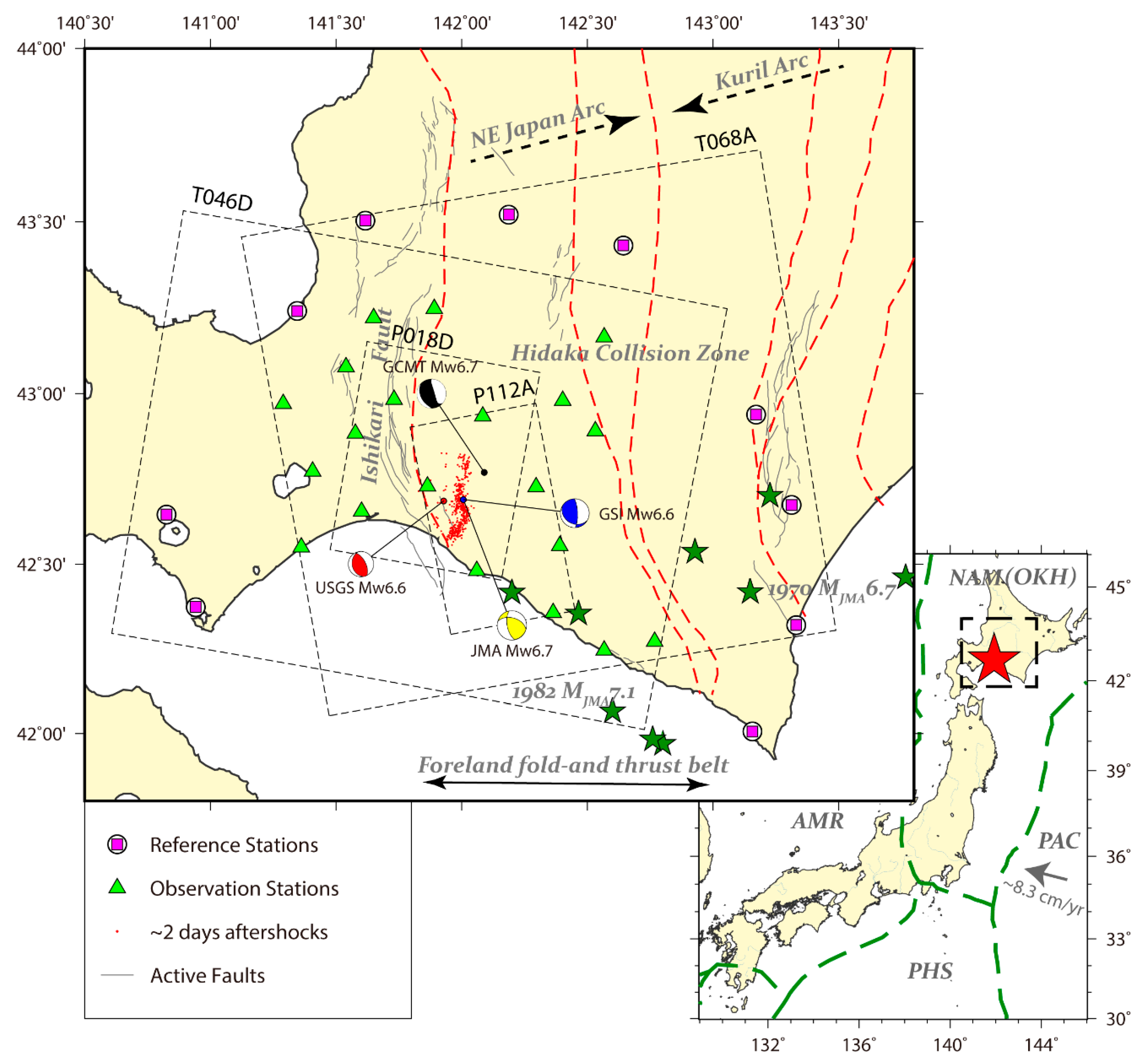
2. Tectonic Background

The Japanese archipelago is located along a complex plate boundary formed by at least four plates (Figure 1). The Pacific plate subducts west-northwestward at a velocity of ~8.3 cm/year beneath the North American plate (or Okhotsk plate) [15]. Southern Hokkaido Island is situated atop the triple junction comprising the northeastern Japan arc, the Kuril arc, and the subducting Pacific plate; this triple junction has been studied by many researchers [16,17,18,19,20]. The oblique subduction of the Pacific plate beneath the Kuril forearc should be responsible for the southwestward migration of the latter [5]. Moreover, the Hidaka Collision Zone (Figure 1), a north-south-trending Cenozoic foreland fold-and-thrust belt was formed westward of it, is currently convergent as a result of the collision between the Kuril arc and northeastern Japan arc [21,22,23]. Although a large amount of crustal deformation within the framework of plate tectonic movement is being absorbed by this fold-and-thrust belt, relatively little seismicity is observed in the crust beneath the fold-and-thrust belt; this may imply that the deformation of the thick sedimentary suite in this region has progressed anelastically [21].

The M > 6.5 earthquakes recorded within and around the Hidaka Collision Zone since 1922 (during the recorded history of the JMA) are mapped in Figure 1. Because inland earthquakes generally do not originate in the lower crust, where rock deforms plastically [20], the depths of these events, for example, the 1970 M_JMA 6.7 Hidaka earthquake that occurred at a depth between 20 and 30 km [24,25] and the 1982 M_JMA 7.1 Urakawa-oki earthquake that occurred at 18–35 km [26], are anomalously deeper than those of typical inland earthquakes. Additionally, according to Omuralieva et al. [27], the average focal depth of inland earthquakes recorded throughout the Japanese islands is approximately 15 km. The 2018 Mw 6.6 inland-type earthquake, which occurred along a blind fault, was also reported by Katsumata et al. [2] to have a relatively deep focal depth of approximately 40 km; similarly, the average depth of the aftershocks was reported to be approximately 20 to 40 km. Katsumata et al. [2] proposed a model in which the 2018 Hokkaido eastern Iburi reverse rupture was triggered by a small strike-slip faulting in a stepover segment, according to their relocated aftershocks. Similar events were also reported recently in Iran, a triplet of M ~6 earthquakes on 2017 of Hojedk, Iran occurred on the reverse faults associated with a strike-slip restraining bend, but all of the three main shocks were shallow rupture [28]. Thus, little is known about such an anomalously deep rupture with a stepover segment in the case of reverse thrust faulting for this 2018 Iburi event. Moreover, the 2018 Iburi earthquake may be attributed to the accumulation of stress resulting from the arc–arc collision process [10]. Thus, this Mw 6.6 inland-type reverse earthquake will provide new insights into the seismogenic processes of this area corresponding to the highly deformed folds and thrusts and tectonic deformation of the arc–arc collision zone stretching across Hokkaido Island.

3. Data Overview

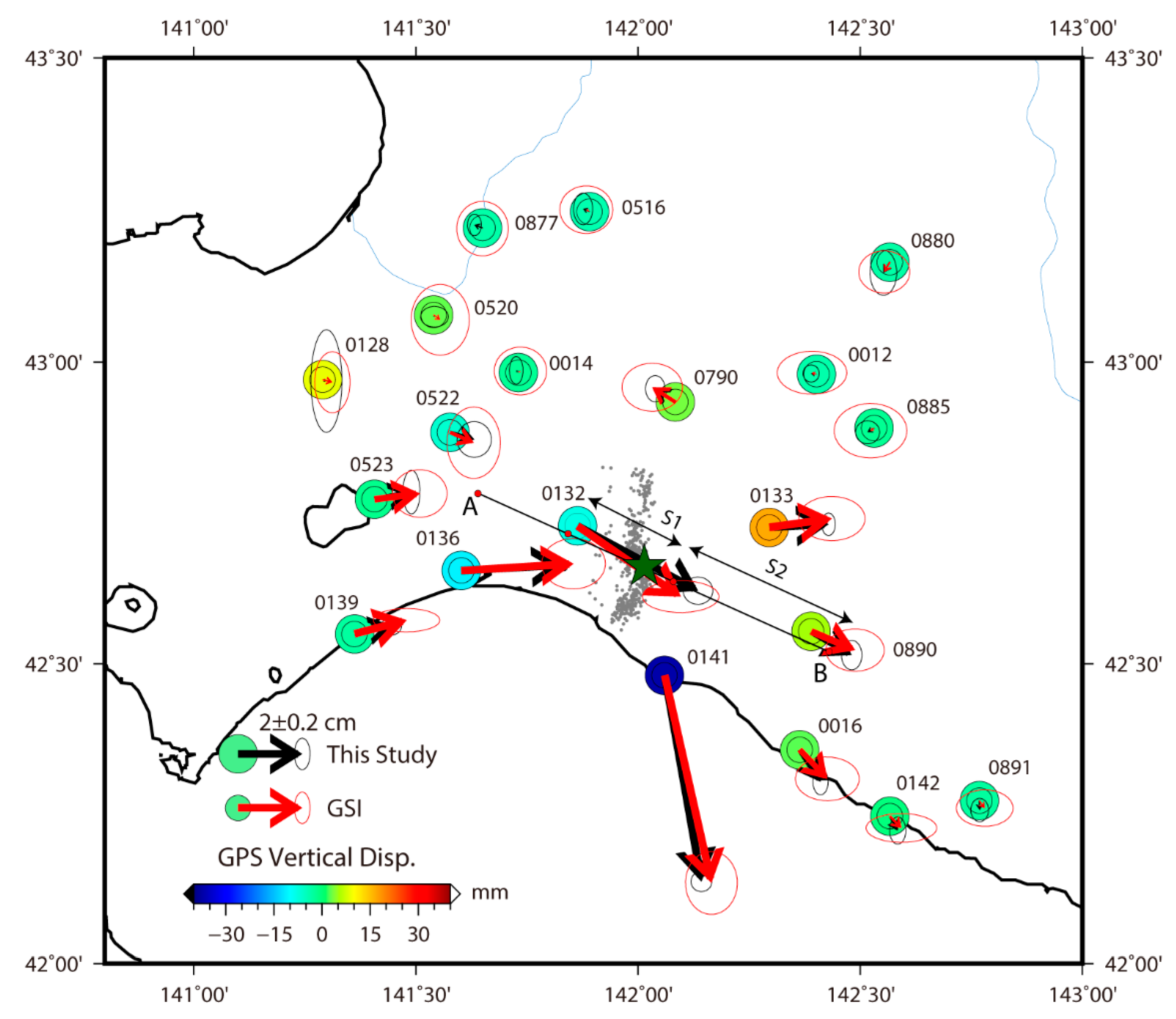
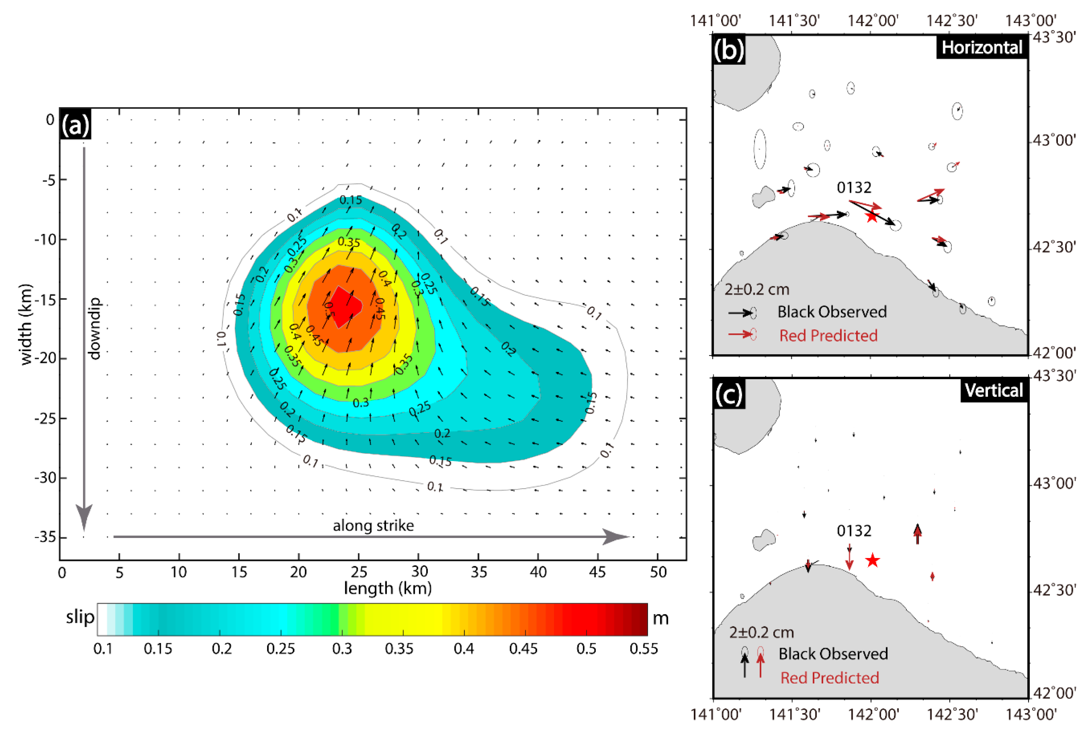
3.1. GPS Observations

Low-rate GPS observations with a sampling interval of 30 s from the GSI GPS Earth Observation Network (GEONET) were processed using GPS at Massachusetts Institute of Technology/Global Kalman filter (GAMIT/GLOBK) software, developed primarily by Massachusetts Institute of Technology (Cambridge, Massachusetts, USA) [29]. During the baseline calculation, the parameters were set as follows: the baseline mode was established for the satellite orbit; the updated Vienna Mapping Function 1 (VMF1) [30] was used to reduce the tropospheric delay error; first-order ionospheric effects were removed by applying an observable ionosphere-free linear combination (LC); ocean tidal loading corrections were implemented using the Finite Element Solutions 2004 (FES2004) tidal model; and the Earth’s tides and solar radiation were considered following the International Earth Rotation and Reference Systems Service 2003 (IERS2003) model and the Berne model, respectively. However, considering the GPS network structure for the global Kalman filter process, it is difficult to select suitable International GNSS Service (IGS) stations as reference stations. Thus, 10 regional GPS stations that were unaffected by coseismic deformation during the 2018 event were chosen as reference stations (Figure 1), and the pre-earthquake seven-day static solutions from these stations were combined to perform the overall adjustment [29]. The GPS time series were averaged separately over the four days before the earthquake (1–4 September) and the four days after the earthquake (6–9 September) to derive the static coseismic displacement solution (Figure 2 and Table S1).

Clear coseismic displacements were recorded by the GPS stations in the vicinity of the epicenter with a reasonable azimuthal coverage; the maximum horizontal and vertical displacements were 6.5 cm and −3.7 cm, respectively. The static coseismic displacement field corresponds well with the focal mechanism of a blind reverse-slip fault with a high dip angle. The coseismic deformation map is also broadly consistent with the GSI results, and the average horizontal and vertical uncertainties (1σ) from this study are 1.6 and 6.2 mm, respectively, which are slightly better than those of the GSI solution (Figure 2).

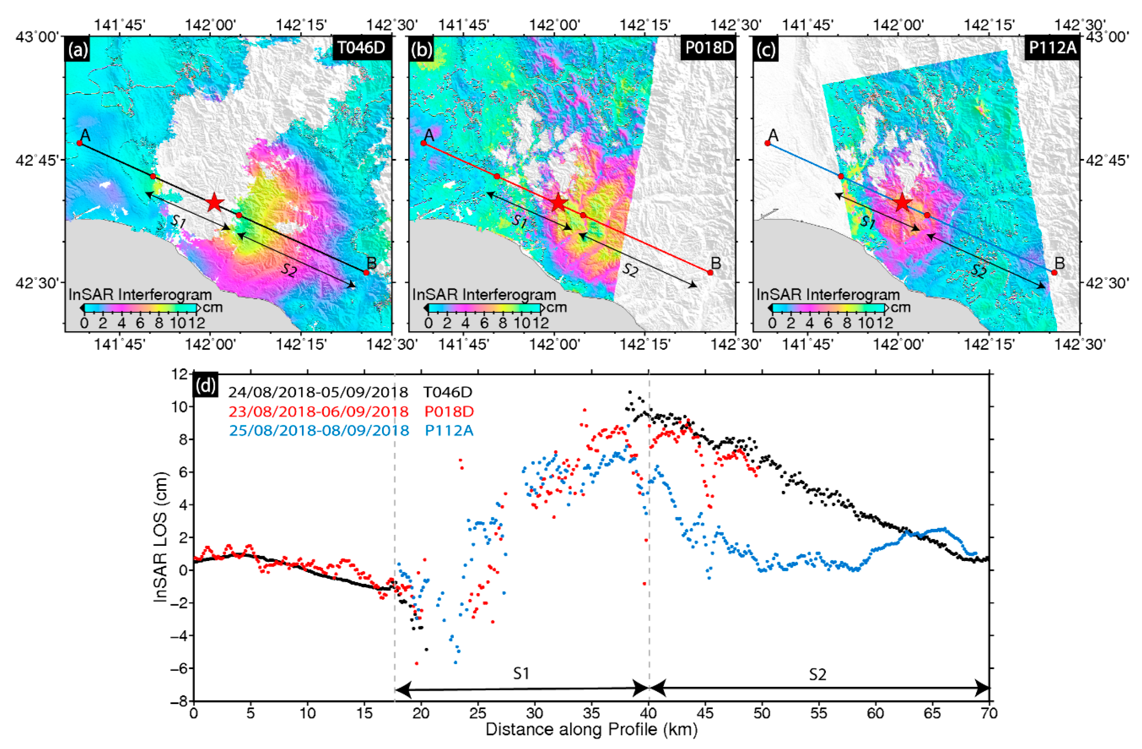
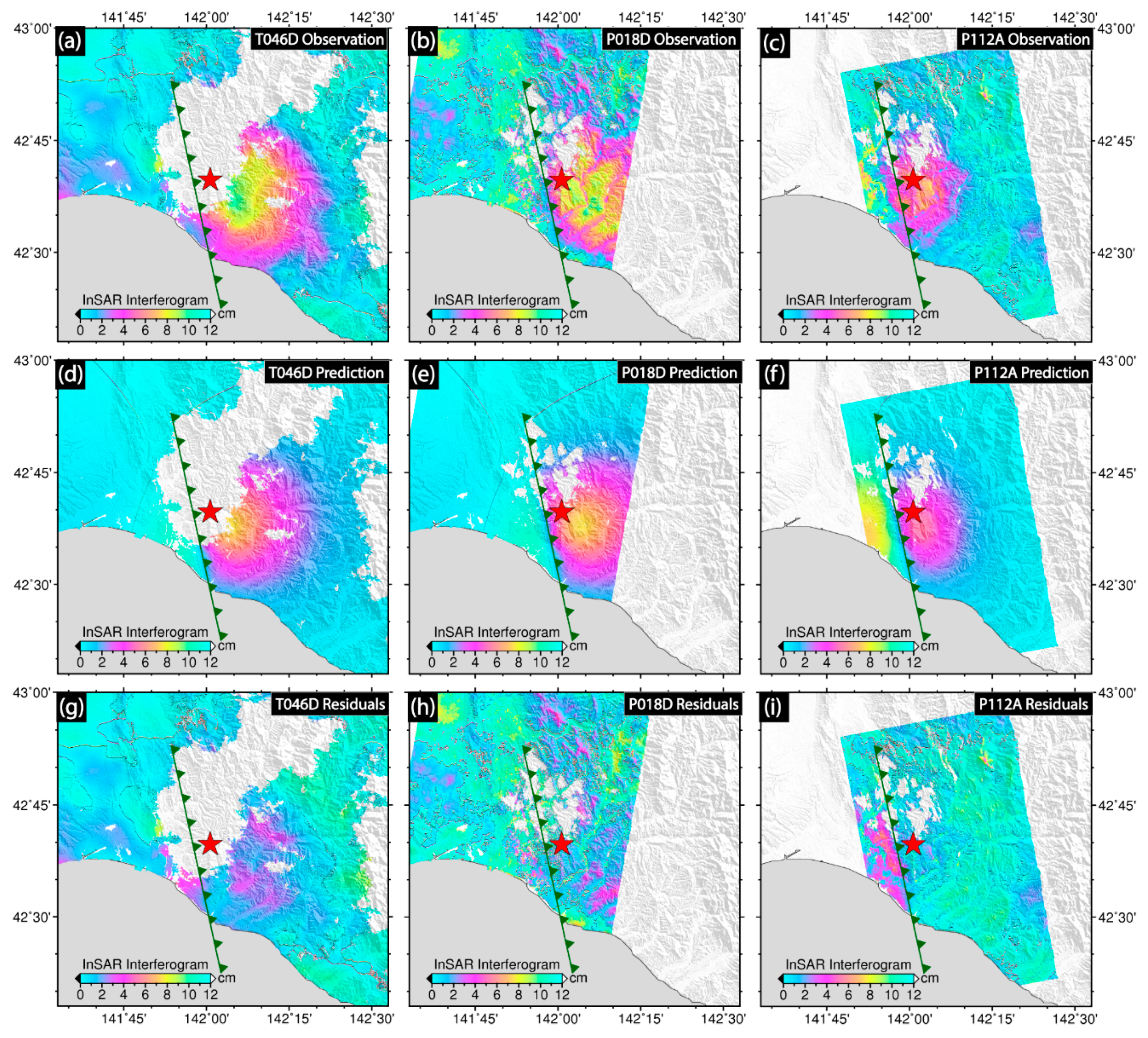
3.2. InSAR Observations

We collected two interferometric pairs of Sentinel-1 images acquired in Terrain Observation with Progressive Scans (TOPS) mode along ascending track T068A and descending track T046D; we also obtained two interferometric pairs of ALOS-2 images in Phased Array L-band Synthetic Aperture Radar-2 (PALSAR-2) stripmap mode along ascending track P112A and descending track P018D (

Table 2. InSAR data parameters used in this study.

No.	Satellite	Track	Master	Slave	${\mathit{B}}_{\perp }$	Inc.	Azi.	$\mathit{\sigma }$†	$\mathit{\alpha }$‡
			YY/MM/DD	YY/MM/DD	m	(°)	(°)	(mm)	(km)
1	Sentinel-1A	T046D	2018/08/24	2018/09/05	45.8	36.4	−169.6	14.3	3.4
2	ALOS-2	P018D	2018/08/23	2018/09/06	69.3	36.2	−169.7	14.5	2.3
3	ALOS-2	P112A	2018/08/25	2018/09/08	−70.6	31.1	−10.9	10.0	2.1
4 *	Sentinel-1B	T068A	2018/09/01	2018/09/13	22.3	41.2	−10.3	9.8	3.4

^† Standard deviations calculated with data from the nondeforming area. ^‡ E-folding correlation length scale of the 1D covariance function. * This image was not used in the nonlinear and linear inversions (see Section 3.3, agreement between global positioning system (GPS) and InSAR observations). Inc.: incidence; Azi.: azimuth; ALOS-2: Advanced Land Observation Satellite-2.

). The Sentinel-1 SAR data and ALOS-2 PALSAR-2 data were processed using the GAMMA InSAR processing software [31], following the InSAR data processing strategies of Wen et al. [32]. The rewrapped coseismic interferograms from the ascending and descending tracks of the Sentinel-1 and ALOS-2 images are shown in Figure 3 and Figure S1. The ALOS-2 interferometry provided better coherence than the Sentinel-1 interferometry for the Iburi earthquake; this is possibly attributable to the former having a longer wavelength. However, the surface deformation is clearly visible from both ascending and descending interferograms, and the main coseismic deformation corresponds well with the mechanism of a thrust event (Figure 3). The relative maximum line-of-sight (LOS) displacements are 11.6, 7.0, 19.9, and 16.7 cm for the T046D, T068A, P018D, and P112A interferograms, respectively. The discrepancies between the two descending and ascending interferograms can be attributed to the incoherent epicentral area among the Sentinel-1 images and the different look angles between Sentinel-1 and ALOS-2 (Table 2).

The differences in the LOS displacements between the ascending and descending tracks can be attributed mainly to the east–west component. The LOS displacements in the T046D and P018D interferograms are in good agreement with those in the P112A interferogram on segment S1 (Figure 3d). This concurrence may indicate that the deformation near the epicenter comprises mainly vertical movement, which is consistent with the characteristics of the near-field deformation of thrust-type earthquakes. On the relatively far-field segment S2 (Figure 3d), the difference between the ascending and descending images may be because of the decrease in vertical displacement far from the epicenter, while the east–west component may play a more important role in the displacement field, which also corresponds well with the GPS observations (Figure 2) and the 2.5D (quasi-eastward and quasi-upward) deformation field (Figure S2). Our 2.5D deformation field derived from the ascending and descending ALOS-2 SAR data (P112A and P018D) uplifted to ~8 cm in the vicinity of the source region, while the distinct eastward displacement to the east of the source is ~5 cm, which is in good agreement with the 2.5D analysis of Kobayashi et al. [33].

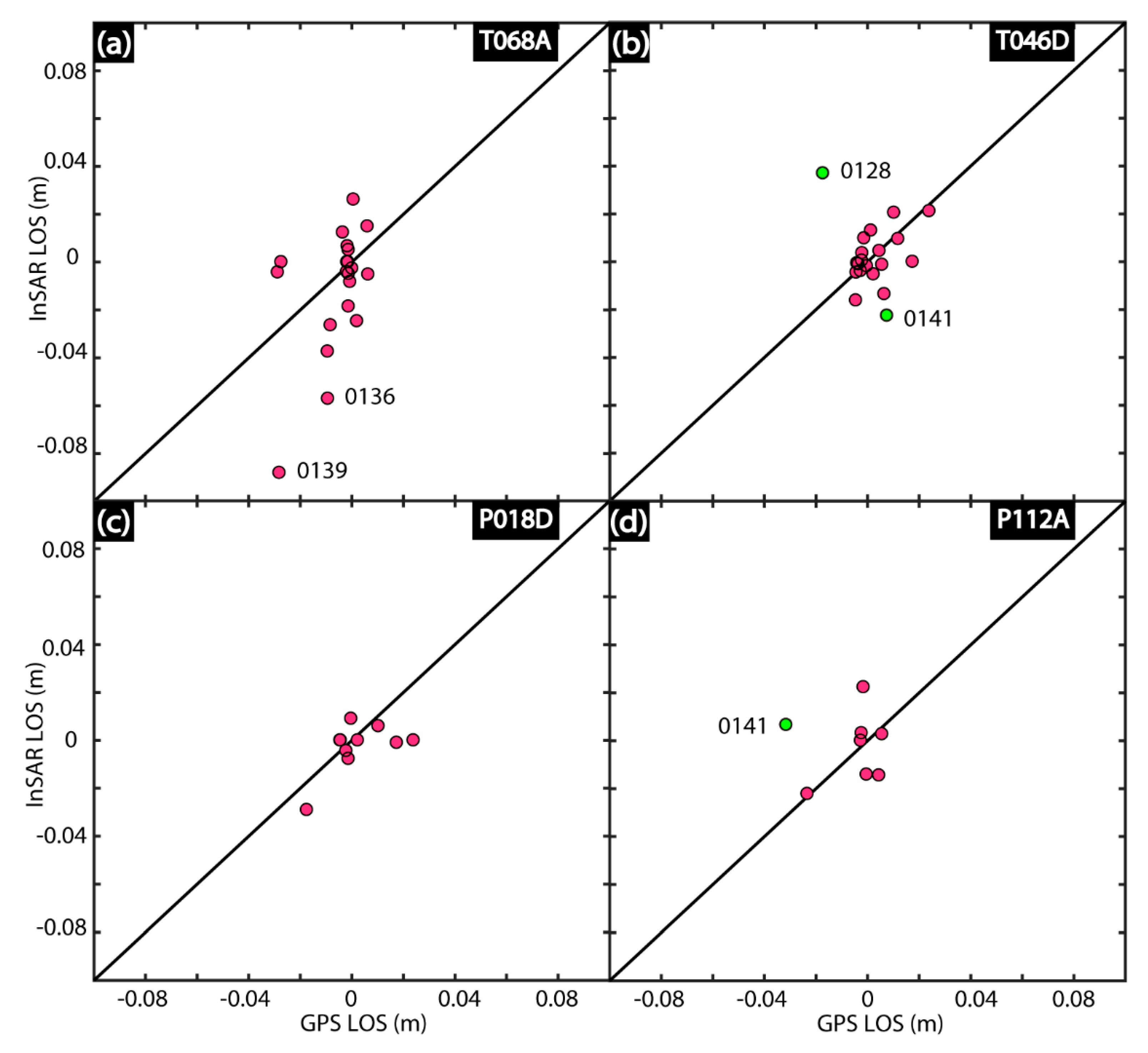
3.3. Agreement between GPS and InSAR Observations

The observed inconsistencies between the different datasets could be because of systematic errors and observation noise, both of which are inevitable. Thus, the three-component GPS displacements ($U_e,U_n,\mathrm{and}{U}_u$) were projected onto the satellite look direction ($d_{los}$) to carry out a comparison between the SAR deformation observations and GPS data. The projection equation can be expressed as follows:

$$d_{los}=-U_{e}cos\phi sin\theta +U_{n}sin\phi sin\theta +U_{u}cos\theta ,$$

(1)

where $\phi$ and $\theta$ represent the azimuth of the satellite heading vector and the radar incidence angle at the reference point, respectively. The lowest consistency was found between the Sentinel-1 T068A interferogram and GPS data (Figure 4a), which may be because of atmospheric noise in the interferogram (Figure S1) or a greater amount of early afterslip in T068A than in the other images, because the repeat pass of T068A was collected eight days (13 September) after the event (Table 2). However, the joint inversion of different datasets with large discrepancies tends to be tricky and unreliable. Therefore, regardless of the cause, we consider the T068A interferogram to be unsuitable for modeling the coseismic source process and, therefore, we eliminated this interferogram from the subsequent inversions. Furthermore, to ensure the overall consistency between the InSAR and GPS datasets, we also eliminated the data from two GPS sites (0128 and 0141) simply by following the criterion $\left|{\mathrm{InSAR}}_{\mathrm{los}}-{\mathrm{GPS}}_{\mathrm{los}}\right|\ge 3\mathrm{cm}$ (Figure 4b–d), where ${\mathrm{InSAR}}_{\mathrm{los}}$ and ${\mathrm{GPS}}_{\mathrm{los}}$ indicate the InSAR-observed and GPS-projected LOS displacements, respectively.

Actually, site 0141 shows the most deformation among all GPS sites. We derived the 2.5D surface deformation field (Figure S2) from the ascending and descending ALOS-2 SAR data (P112A and P018D), because it could provide additional insight in possible sources of the discrepancies observed between the different data sources. From the quasi-upward map (Figure S2b), we observe the possible local ground subsidence at site 0141, which was also reported in Kobayashi et al. [33]. Furthermore, Kobayashi et al. [33] also reported that the mounting pillars at the near-field sites 0141 are tilted slightly as a result of the earthquake. Thus, site 0141 showing the most deformation should not be involved in the inversions.

3.4. Data Reduction and Weighting

InSAR data comprise several millions of pixels, so it is quite uneconomical to invert a source model using all available observations. Thus, to downsample the InSAR differential interferograms and improve the computational efficiency of the inversion, the resolution-based quadtree sampling approach [34] was adopted to avoid the effect of far-field observation errors. The number of InSAR data points among the three interferograms was reduced from millions of observations to 2014 points (Figure S3). During the inversions, we also employed the Helmert variance component estimation (HVCE) method suggested by Xu et al. [35] to determine the weighting of each dataset, owing to its various advantages in a joint inversion with several different datasets.

4. Nonlinear Optimization and Source Modeling

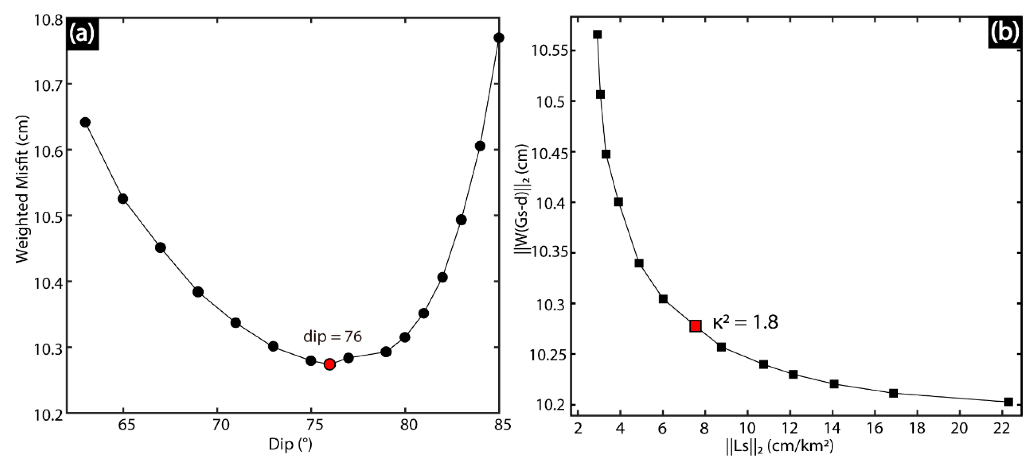
4.1. Nonlinear Inversion

We inverted the InSAR and GPS observations with a two-step approach: a nonlinear inversion was performed to invert for nine fault parameters (including the location, strike, dip, length, depth, width, and slip) with uniform slip; then, a linear inversion was implemented to retrieve the slip distribution along the fault plane. The multipeak particle swarm optimization (M-PSO) approach, which is based on a hybrid minimization algorithm [36], was used to perform the nonlinear inversion. We modeled the 2018 Hokkaido eastern Iburi earthquake as a single rectangular dislocation [37] in a homogeneous, isotropic elastic half-space assuming a Poisson ratio of 0.25 and a shear modulus of $3.32\times {10}^{10}\mathrm{N}/{\mathrm{m}}^2$ [38]. During the inversion, the starting values for the relative weight ratio among the InSAR (T046D, P018D and P112A) and GPS datasets were given as 0.293:0.290:0.420:1.000 based on the variances (standard deviations) of the three interferograms and GPS data. After a few iterations, the variances of the unit weight became almost uniform for all three InSAR interferograms, and the relative weight ratio converged to 0.260:0.216:0.263:1.000. Next, the model solutions from 100 simulations perturbed with observation noise based on the variance–covariance matrix of the three interferograms and the variance of the GPS data were employed to estimate the standard deviations from the model distributions with a Monte Carlo bootstrap simulation technique [39]. We set bounds for the source parameters (Table S2) by referring to the GSI fault parameters and focal mechanisms, which were also derived from a joint inversion of InSAR and GNSS data. Initially, we inverted the datasets with an unconstrained fault length and width for uniform slip on an east-dipping fault plane, but the solutions yielded high slip (>5000 m) along a fault with an implausible length and width. Therefore, we fixed the width to 14 km, which is also largely consistent with the GSI fault width (Table 1), according to the empirical relationships of Wells and Coppersmith [40].

Table 1 shows all the inverted fault parameters and their errors, and Figure S4 gives the means and standard deviations of the fault parameters calculated by the Monte Carlo method. In general, the inverted fault parameters correspond well with the GIS results, and their errors may be attributed to observation noise. We also inverted the west-dipping southeast-trending fault plane, but the inversion results did not converge. These inversion results suggest that the fault is a blind NNW-trending, east-dipping thrust fault, which is consistent with the focal mechanisms derived from the USGS, GCMT, and GSI. In addition, the inverted geodetic moment magnitude of the 2018 event is Mw 6.44 ($M_0=5.06\times {10}^{18}\mathrm{N}\mathrm{m}$), which is somewhat smaller than the estimates of Mw 6.6 from the USGS and Mw 6.7 from the GCMT and JMA, which were derived from the inversion of seismic data, and slightly smaller than the estimate of Mw 6.56 from the GSI, which was derived from the joint inversion of InSAR and GNSS data. The small differences of derived magnitude may be partially a result of the inconsistencies between the geodetic and seismic data (Table 1).

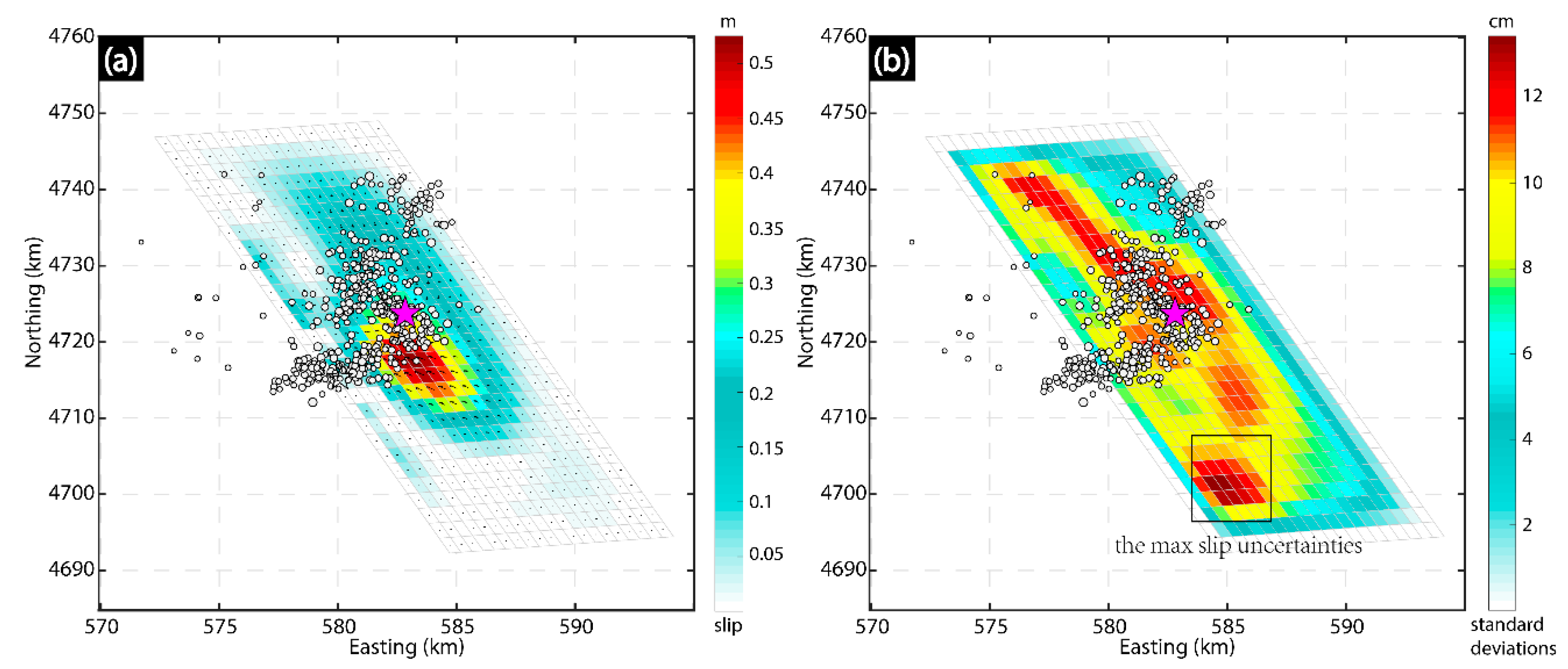
4.2. Linear Inversion

On the basis of the fault parameters determined by the abovementioned nonlinear optimization, we performed a linear inversion with the conjugate gradient least squares method [41]. To determine the slip distribution along the fault plane, we fixed the fault geometry derived from the uniform slip modeling and extended the along-strike fault length to 56 km and the downdip fault width to 40 km; furthermore, we divided the fault plane into patches with sizes of 2 × 2 km. A nonnegativity constraint was imposed to allow only reverse slip during the slip inversions.

We found that the fault model with a dip angle of 76° fits the LOS displacements from all three tracks and the GPS data very well (Figure 5a) when a smoothing factor of 1.8 was chosen (Figure 5b). The optimal slip model was obtained by minimizing the misfit between the observed surface deformation and the modeled deformations with the optimal smoothing factor:

$$\varnothing =\min (\Vert W{\left(Gs-d\right)\Vert }_2+{\kappa }^2\Vert Ls{\Vert }_2),$$

(2)

where ${\Vert \Vert }_2$ represents the Euclidean norm ($L^2$ norm), W is the weighted matrix from the variance–covariance matrix, G is the surface deformation response to unit slip on the fault plane (Green’s function), s is the slip component of each patch, d is the observation vector, and L is the Laplacian second-order finite difference operator. An optimal smoothing factor of κ² = 1.8 was chosen in the inversion according to the trade-off curve shown in Figure 5b. We regularized the inversion problem by requiring no slip at the fault edges. Our preferred slip model features a heterogeneous slip pattern with a significant slip area extending 30 km along the strike and 25 km in the downdip direction; the peak slip magnitude approaches 0.53 m at a depth of 15.5 km with strike-slip and dip-slip components of 0.22 m and 0.48 m, respectively (Figure 6 and Figure 7a). In addition to the main slip, the shallow part of the fault (0–5 km), which features a blind reverse-slip fault rupture, has no apparent slip (Figure 7a). Our 3D slip model is illustrated in the Supplementary Materials as Figure S5 and the slip distribution in digital format is documented in Table S3. The estimated geodetic moment magnitude released by the distributed slip model is $6.16\times {10}^{18}\mathrm{N}\mathrm{m}$, which corresponds to an event magnitude of Mw 6.50. The average slip uncertainty of the optimal slip distribution is 6.5 cm, and the maximum slip uncertainty for the slip patches is 13.4 cm (Figure 6b); however, we suggest that this value is somewhat unreasonable. Accordingly, we then carried out forward modeling to determine the source of the maximum slip uncertainty (Figure S6). The results show that the maximum slip uncertainty on the fault plane corresponds to the observations at ~42.50 °N and 142.05 °E. We found that the downsampling observations in this region are relatively sparse (Figure S3); thus, the maximum slip uncertainties may be attributable to the scarcity of observations, the presence of observation noise, or possible model errors.

The resolution tests were also performed to systematically verify the reliability of our preferred distributed slip model. The shallow (Figure S7a–c), middle (Figure S7d–f), deep slip (Figure S7g–i), and classical checkerboard tests (Figure S7j–l) were carried out to invert the synthetic models and study how well the inversion slip is resolved. These tests suggested that the long wavelength features are well recovered at the shallow (<10 km) and middle depth (<20 km) (Figure S7a–f), while the long wavelength features at greater depth (>30 km) (Figure S7g–i) and shorter wavelength features at middle depth (>20 km) (Figure S7j–l) could not be restricted sufficiently. The low resolving ability at larger depth is intrinsic when inverted form surface displacement data (e.g., GPS, InSAR) based on elastic dislocation theory, according to previous studies (e.g., Bos and Spakman [42], Peyret et al. [43]). Because our preferred slip model features one long-wavelength asperity at the depths of 10–25 km, which is plausibly consistent with the surface deformation obtained from the coseismic InSAR interferograms (Figure 3 and Figure S2), we can indicate that the main slip pattern of this event can be constrained relatively well by existing data.

The GPS data observations are plausibly consistent with the predictions except for the horizontal and vertical displacements of a few near-field stations (e.g., 0132), the displacements at which were predicted somewhat poorly (Figure 7b,c); the poor prediction quality at 0132 station may be related to the slight tilt of the mounting pillar [33] and the simple single-fault model may also be responsible for the poor fitting of GPS sites (discussion detailed in Section 5.2.1). With regard to the InSAR fitting results, both the Sentinel-1 T046D and the ALOS-2 P018D interferograms fit largely well (Figure 8), except for some localized higher misfit for the ALOS-2 P112A interferogram along the assumed fault trace at the surface (Figure 8i). These local misfits could be the result of phase unwrapping errors of the P112A image or also an oversimplification of the fault geometry. In this study, we assume a planar fault plane with a constant dip angle; if the actual fault is listric or if the fault is curved along the strike, then our planar fault model will be inadequate to describe very near-field deformation related to shallower fault slip.

5. Discussion

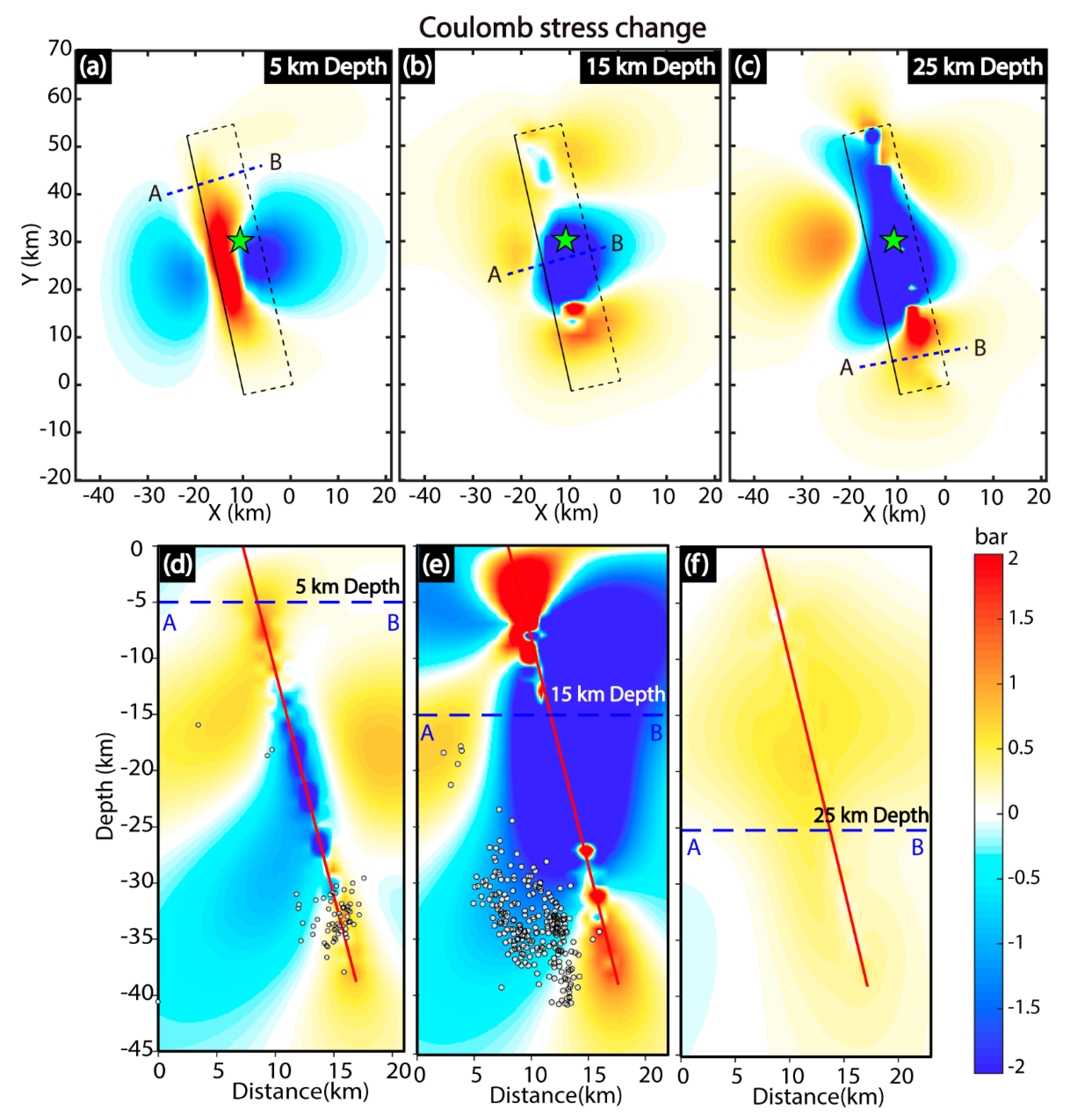
5.1. Static Coulomb Stress Changes and Seismic Hazards

An earthquake rupture is a process of releasing and readjusting stress; accordingly, stress readjustment plays an important role in understanding the seismic hazard in a seismogenic region, as has been reported by many studies [12,32,44,45]. Without taking shallow slip into account, the distributed slip model of the 2018 Hokkaido eastern Iburi earthquake evaluated herein was used to calculate the static Coulomb stress change (ΔCSC) on the fault plane and in the periphery of the study region using Coulomb 3.3 software [46,47], in order to understand the transfer of stress from deep to shallow depths and assess the regional seismic hazards.

5.1.1. Static Coulomb Stress Changes and Aftershock Distributions

The coseismic Coulomb stress changes were calculated at different depths from 5 to 25 km with an interval of 10 km using the optimal rupture plane; the effective coefficient of friction and shear modulus were set to 0.4 and $3.32\times {10}^{10}\mathrm{N}/{\mathrm{m}}^2$ [38], respectively. The receiver fault orientation was the same as the fault orientation for the main shock. The calculation result suggests that the stress increased (promoting future fault rupture) in the shallower section to the north and south of the fault (Figure 9a,d). Yamagishi and Yamazaki [3] reported some deep-seated dip-slip landslides to the southeast of the epicenter, possibly because of this increase in ΔCSC. Moreover, the occurrence of deep-seated landslides may be related to the differences in rheology between different types of rocks [48]. The Coulomb stresses decreased at a depth of 15 km within the main rupture area (Figure 9b), producing the maximum slip. The ΔCSC values at different depths at the southern end of the fault are almost positive (Figure 9c,f), which suggests that the future failure may be brought closer in this area in the future.

As shown in Figure 9d,e, the distribution of relocated aftershocks at a depth of ~20 km is generally consistent with the static stress trigger theory. However, at a depth of ~30 km, the far-field relocated aftershocks correspond well to the positive ΔCSC (Figure 9d); while we did not observe good agreements between the near-field aftershocks and the static stress shadow at this depth (Figure 9e). The inconsistencies between the ΔCSC and the deep aftershocks’ distribution may have resulted from the slip model error. Our resolution tests suggest that the fault slip distribution could not be resolved sufficiently at the depth ~30 km (Figure S7g–i), which could be attributed to the intrinsically ill-conditioned inverse problem of retrieving fault slip with geodetic data only [42,43]. Hong et al. [49] also suggested that the ΔCSC in the near-field of the fault may be unreliable, because of the limitation of the dislocation model based on linear elasticity. Therefore, owing to the large depth of the aftershocks (the average depth of the aftershocks was ~30 km [2]), we argue that the relation between the distribution of aftershocks and the ΔCSC should be investigated carefully with a refined distributed slip model, which should be constrained by a variety of datasets (e.g., geodetic, seismic and geological data) in further studies.

Previous studies also reported that other triggering mechanisms may be also active, except for the static stress trigger theory. For example, Parsons [50] demonstrated the plausibility of dynamic stress (temporary stress changes associated with earthquake shaking) triggering leading to aftershock decay. Felzer and Brodsky [51] inferred that aftershocks may be driven by a mix of both dynamic and static stress changes. Furthermore, shear stress changes and the invariants of the stress tensor could better explain the aftershock patterns than could the ΔCSC, as reported by several previous studies [52,53,54]. Thus, further research is also needed to reveal the dominant triggering mechanism of the aftershocks following the 2018 Hokkaido eastern Iburi event.

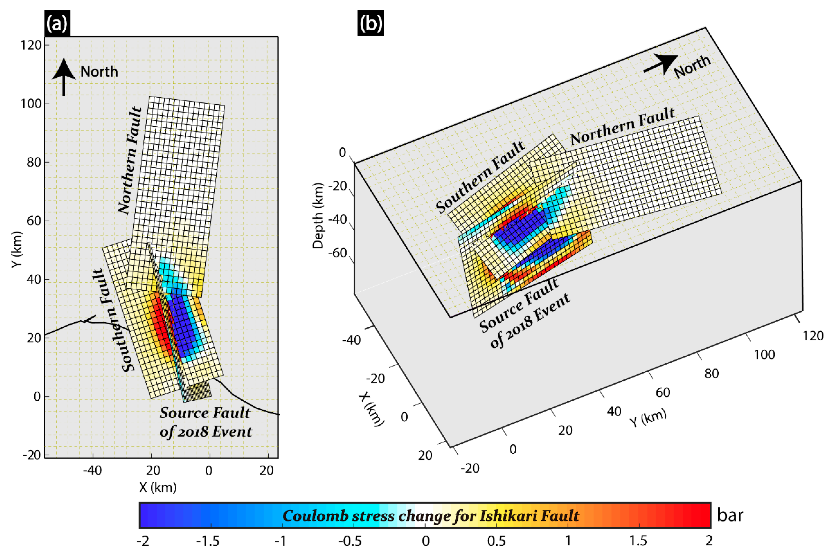
5.1.2. Static Coulomb Stress Changes on the Surrounding Faults

There is an active fault called Ishikari fault zone near the source region of the Hokkaido Iburi earthquake (Figure 1). The Ishikari fault is divided into northern and southern parts, both of the two parts could be capable of producing M ~7.8 earthquakes [10]. Therefore, the stress disturbance at the northern and southern Ishikari faults were calculated to evaluate the earthquake potentiality. The source parameters of the northern and southern Ishikari faults were from Ohtani and Imanish [10] and the effective coefficient of friction and shear modulus were set to be 0.4 and $3.32\times {10}^{10}\mathrm{N}/{\mathrm{m}}^2$ [38]. Our result shows that the ΔCSC of the southern half of the northern fault ranges from −1.40 to 0.90 bar (Figure 10), because the most recent event is restricted to the central part of the northern fault and has not been found on the southern part [10], so a high seismic potential remains there. The intersection of the source fault of 2018 Iburi event and the southern Ishikari fault suggested a high positive ΔCSC (Figure 10), which is also in good agreement with the results published recently by Kobayashi et al. [33]. The value of the ΔCSC along the southern Ishikari fault ranges from −15.06 to 11.38 bar, which is larger than the ΔCSC of the northern Ishikari fault (Figure 10). However, little is known about the recurrence interval and the elapsed time of the last event, which makes it difficult for us to assess the seismic hazards of this fault [10]. Overall, the positive ΔCSC values may indicate the Ishikari fault may be brought closer to rupture as a result of the 2018 Iburi earthquake. Moreover, Ohtani and Imanish [10] also calculated the Coulomb stress change of the Iburi earthquake to evaluate the seismic potential of the Ishikari fault, based on seismological analysis and numerical simulations. They took the postseismic viscoelastic relaxation into account and also argued that the northern and southern Ishikari faults are under increasing seismic threat after the Iburi earthquake. Therefore, we suggest that more attention should be paid to potential earthquake disasters in this region in the near future, together with seismicity (M ~6.5) of the Ishikari fault being low [21] (Figure 1).

5.2. Seismogenic Structure and Tectonics Setting

5.2.1. Possible Complexity of the Seismogenic Fault

The multi-fault system should be investigated in further studies. Even though the InSAR interferograms were fit largely well by the single-fault model (Figure 8), the misfit of a few GPS sites is somewhat significant (Figure 7b,c). The visually poor fitting of GPS stations is also observed in the study of Kobayashi et al. [33], in which a single fault was used, while the GPS fitting is improved when a two-fault rupture was taken into account [14]. Katsumata et al. [2] also proposed a fault system in which the 2018 reverse event was located at a small strike-slip fault in the stepover segment, according to the relocated aftershocks’ distribution. Kobayashi et al. [14] inverted the rupture progress using strong motion and GPS data, their results showed that the minor rupture initiated on the minor fault plane around the main shock (~40 km) and the major fault started to rupture 4–6 s after the rupture initiation. The slip pattern of their rupture model is similar to that proposed in this study, though their maximum slip is up to 2.9 m. However, the minor deep fault parameters of both of the above proposed multi-fault models have not be determined precisely. In consideration of the greater depth (~40 km) of the main shock, some slip indeed should be produced therein. However, according to previous studies (e.g., Bos and Spakman [42], Peyret et al. [43]) and our resolution tests (Figure S7), the spatial distribution of fault slip at a large depth could not be resolved sufficiently with only geodetic data. Furthermore, Kobayashi et al. [33] also speculated the possibility that the seismic fault structurally connects with the Ishikari southern fault, owing to the source fault is geographically close to the southern parts of Ishikari fault. In this case, the fault’s high dip angle (~70°) at large depth must change to a low dip angle (~30°) at a shallow depth (~10 km), but detailed information on regional crustal structures is needed to deepen the discussion of this speculation in the future. However, we argue the main slip pattern of the fault plane may not change significantly if the two faults are physically connected at shallow depth, because the main shock mainly attributed to a deep high-dip reverse faulting. We, therefore, argue the convinced determination of the faults geometry and refined slip distribution should be integrated with additional data (e.g., geological, source mechanism, P-wave backprojection, strong motion data) and particularly with the regional geologic framework, which is of great significance for a better understanding of the stress changes and potential future hazards.

5.2.2. Seismotectonics and Seismogenesis

Complex seismogenic structures may be related to complex seismotectonics and seismogenesis in Hokkaido region. Hokkaido Island is subjected to high compressional stresses resulting from the collision between the North American (Okhotsk) and Eurasian plates and the collision between the northeastern Japan arc and Kuril arc; this tectonic regime is considered to be responsible for the uplift of the metamorphic rocks forming the Hidaka Collision Zone [21] (Figure 1). Several deep inland damaging earthquakes have occurred in this region, for example, the 1982 M_JMA 7.1 and 1970 M_JMA 6.7 thrust events [19,20,55] (Figure 1). Kita et al. [19,55] investigated the relationship between these two M ~7 deep inland events in Hokkaido Island and the corresponding collision processes by investigating the seismic velocity and seismic attenuation structures. They found that the fault planes of these two events correspond to the boundary between mantle material and crustal material, and the M 7 class earthquakes may be attributed to the arc-arc collision of the NE Japan and Kuril forearcs [55]. The 2018 Hokkaido eastern Iburi earthquake was also an anomalously deep intraplate event with a focal depth of approximately 40 km [2]. Kobayashi et al. [33] investigated the velocity structure in and around the focal area. Their result shows the 2018 earthquake also occurred at a seismic velocity boundary, which is also consistent with the high-dip angle fault plane and the aftershocks’ distribution. Therefore, the rupture of the 2018 event occurred at the boundary between mantle material and crustal material may have been triggered by the ongoing arc–arc collision between the northeastern Japan and Kuril forearcs, similar to the 1982 and 1970 M ~7 events [55].

Kita et al. [19] also proposed a model for the subsurface structure and geodynamic processes beneath Hokkaido that suggested the possible existence of geofluids and regions where earthquakes occur due to excess pore fluid pressure. These geofluids may be released into the mantle wedge from the subducted Pacific slab by slab dehydration at depths ranging from 110 to 130 km. The depth to the subducted Pacific slab at the epicenter of the 2018 event is approximately 100 km [56]. Kita et al. [19] suggested that geofluids most likely reach the Moho in this region; the 3D electrical resistivity modeling of Ichihara et al. [20] also favored the existence of fluid flow in this region, possibly contributing to overpressurized conduction, which produces deep inland reverse-type earthquakes. Therefore, the formation of the 2018 earthquake may be closely related to the subsurface existence of geofluids.

Evidently, Hokkaido Island exhibits a complex tectonic and geophysical seismogenesis. However, the regional M ~7 events above-mentioned show similar seismogenic patterns (arc–arc collision, seismic velocity boundary, and involvement of geofluid), the 2018 event will shed new lights on the regional seismotectonics and seismogenesis. Furthermore, the 2018 inland-type earthquakes are closer to the Ishikari faults which could be capable of triggering M ~7.8 earthquakes [10], thus the investigations of the complex subsurface structure (e.g., arc-arc collision, seismic velocity boundary, and involvement of geofluid) also are significant for understanding the seismic hazard in the area.

6. Conclusions

Sentinel-1 and ALOS-2 InSAR and GPS data were used to jointly invert the source parameters and fault slip distribution of the Mw 6.6 Hokkaido eastern Iburi, Japan, earthquake that occurred on 5 September 2018. First, we carried out a nonlinear inversion to invert for nine fault parameters, the result of which shows that the seismogenic fault was a blind NNW-trending (strike angle ~347.2°), east-dipping (dip angle ~79.6°) thrust fault. The inverted geodetic moment magnitude of the 2018 event is Mw 6.44 ($M_0=5.06\times {10}^{18}\mathrm{N}·\mathrm{m}$). Then, a linear inversion was performed based on the optimal fault geometry derived from the nonlinear optimization. The linear inversion suggests that a significant slip area extends 30 km along the strike and 25 km in the downdip direction and that the peak slip magnitude can approach 0.53 m at a depth of 15.5 km with strike-slip and dip-slip components of 0.22 m and 0.48 m, respectively. The estimated geodetic moment magnitude released by the distributed slip model is $6.16\times {10}^{18}\mathrm{N}·\mathrm{m}$, equivalent to an event magnitude of Mw 6.50. According to the Coulomb stress change at the surrounding faults, more attention should be paid to potential earthquake disasters in this region in the near future. The seismogenic system may be complex and the 2018 event may relate to the complex subsurface structure (e.g., arc–arc collision, seismic velocity boundary, and involvement of geofluid).

References

1. USGS. Available online: https://earthquake.usgs.gov/earthquakes/eventpage/us2000h8ty/executive (accessed on 30 September 2018).
2. Katsumata, K.; Ichiyanagi, M.; Ohzono, M.; Aoyama, H.; Tanaka, R.; Takada, M. The 2018 Hokkaido Eastern Iburi earthquake (MJMA = 6.7) was triggered by a strike-slip faulting in a stepover segment: Insights from the aftershock distribution and the focal mechanism solution of the main shock. Earth Planets Space 2019, 71, 53. [Google Scholar] [CrossRef]
3. Yamagishi, H.; Yamazaki, F. Landslides by the 2018 Hokkaido Iburi-Tobu Earthquake on September 6. Landslides 2018, 15, 2521–2524. [Google Scholar] [CrossRef] [Green Version]
4. Shao, X.; Ma, S.; Xu, C.; Zhang, P.; Wen, B.; Tian, Y. Planet Image-Based Inventorying and Machine Learning-Based Susceptibility Mapping for the Landslides Triggered by the 2018 Mw 6.6 Tomakomai, Japan Earthquake. Remote Sens. 2019, 11, 978. [Google Scholar] [CrossRef]
5. Kimura, G. The latest Cretaceous-early Paleogene rapid growth of accretionary complex and exhumation of high pressure series metamorphic rocks in northwestern Pacific margin. J. Geophys. Res. 1994, 99, 22147–22164. [Google Scholar] [CrossRef]
6. Bird, P. An updated digital model of plate boundaries. Geochem. Geophys. Geosyst. 2003, 4. [Google Scholar] [CrossRef]
7. GCMT. Available online: http://www.globalcmt.org/CMTsearch.html (accessed on 30 September 2018).
8. JMA. Available online: http://www.jma.go.jp/jma/index.html (accessed on 30 September 2018).
9. GSI. Available online: http://www.gsi.go.jp/cais/topic180912-index-e.html (accessed on 30 September 2018).
10. Ohtani, M.; Imanishi, K. Seismic potential around the 2018 Hokkaido Eastern Iburi earthquake assessed considering the viscoelastic relaxation. Earth Planets Space 2019, 71, 57. [Google Scholar] [CrossRef] [Green Version]
11. Wen, Y.; Xu, C.; Liu, Y.; Jiang, G.; He, P. Coseismic slip in the 2010 Yushu earthquake (China), constrained by wide-swath and strip-map InSAR. Nat. Hazards Earth Syst. Sci. 2013, 13, 35–44. [Google Scholar] [CrossRef]
12. Xu, G.; Xu, C.; Wen, Y.; Jiang, G. Source parameters of the 2016–2017 Central Italy earthquake sequence from the Sentinel-1, ALOS-2 and GPS data. Remote Sens. 2017, 9, 1182. [Google Scholar] [CrossRef]
13. Dhakal, Y.P.; Kunugi, T.; Kimura, T.; Suzuki, W.; Aoi, S. Peak ground motions and characteristics of nonlinear site response during the 2018 Mw 6.6 Hokkaido eastern Iburi earthquake. Earth Planets Space 2019, 71, 56. [Google Scholar] [CrossRef]
14. Kobayashi, H.; Koketsu, K.; Miyake, H. Rupture process of the 2018 Hokkaido Eastern Iburi earthquake derived from strong motion and geodetic data. Earth Planets Space 2019, 71, 63. [Google Scholar] [CrossRef]
15. Gripp, A.E.; Gordon, R.G. Young tracks of hotspots and current plate velocities. Geophys. J. Int. 2002, 150, 321–361. [Google Scholar] [CrossRef]
16. Jolivet, L.; Miyashita, S. The Hidaka shear zone (Hokkaido, Japan): Genesis during a right-lateral strike-slip movement. Tectonics 1985, 4, 289–302. [Google Scholar] [CrossRef]
17. Tsumura, N.; Ikawa, H.; Ikawa, T.; Shinoha, M. Delamination-wedge structure beneath the Hidaka collision zone, Central Hokkaido, Japan inferred from seismic reflection profiling. Geophys. Res. Lett. 1999, 26, 1057–1060. [Google Scholar] [CrossRef]
18. Kita, S.; Okada, T.; Hasegawa, A.; Nakajima, J.; Matsuzawa, T. Existence of interplane earthquakes and neutral stress boundary between the upper and lower planes of the double seismic zone beneath Tohoku and Hokkaido, northeastern Japan. Tectonophysics 2010, 496, 68–82. [Google Scholar] [CrossRef]
19. Kita, S.; Nakajima, J.; Hasegawa, A.; Okada, T.; Katsumata, K.; Asano, Y.; Kimura, T. Detailed seismic attenuation structure beneath Hokkaido, northeastern Japan: Arc-arc collision process, arc magmatism, and seismotectonics. J. Geophys. Res. Solid Earth 2014, 119, 6486–6511. [Google Scholar] [CrossRef]
20. Ichihara, H.; Mogi, T.; Tanimoto, K.; Yamaya, Y.; Hashimoto, T. Crustal structure and fluid distribution beneath the southern part of the Hidaka collision zone revealed by 3-D electrical resistivity modeling. Geochem. Geophys. Geosyst. 2016, 17, 1480–1491. [Google Scholar] [CrossRef] [Green Version]
21. Iwasaki, T.; Adachi, K.; Moriya, T.; Miyamachi, H. Upper and middle crustal deformation of an arc-arc collision across Hokkaido, Japan, inferred from seismic refraction/wide-angle reflection experiments. Tcetonophysics 2004, 388, 59–73. [Google Scholar] [CrossRef]
22. Kato, N.; Sato, H.; Orito, M.; Hirakawa, K.; Ikeda, Y.; Ito, T. Has the plate boundary shifted from central Hokkaido to the eastern part of the Sea of Japan? Tectonophysics 2004, 388, 75–84. [Google Scholar] [CrossRef]
23. Van Horne, A.; Sato, H.; Ishiyama, T. Evolution of the Sea of Japan back-arc and some unsolved issues. Tectonophysics 2017, 710, 6–20. [Google Scholar] [CrossRef]
24. Ichikawa, M. Reanalysis of the mechanisms of earthquakes which occurred in and near Japan and statistical studies on the nodal plane solutions obtained, 1926–1968. Geophys. Mag. 1970, 35, 207–273. [Google Scholar]
25. Moriya, T. Aftershock activity of the Hidaka mountains earthquake of 21 January 1970 (in Japanese with English figure captions). J. Seismol. Soc. Jpn. 1972, 24, 287–297. [Google Scholar]
26. Moriya, T.; Miyamachi, H.; Katoh, S. Spatial distribution and mechanism solutions for foreshocks, mainshock and aftershocks of the Urakawa-Oki earthquake of 21 March 1982 (in Japanese with English figure captions). Geophys. Bull. Hokkaido Univ. 1983, 42, 191–213. [Google Scholar]
27. Omuralieva, A.M.; Hasegawa, A.; Matsuzawa, T.; Nakajima, J.; Okada, T. Tectonophysics Lateral variation of the cutoff depth of shallow earthquakes beneath the Japan Islands and its implications for seismogenesis. Tectonophysics 2012, 518, 93–105. [Google Scholar] [CrossRef]
28. Savidge, E.; Nissen, E.; Nemati, M.; Karas, E.; Hollingsworth, J.; Talebian, M.; Bergman, E.; Ghods, A.; Ghorashi, M.; Kosari, E.; et al. The December 2017 Hojedk (Iran) earthquake triplet-sequential rupture of shallow reverse faults in a strike-slip restraining bend. Geophys. J. Int. 2019, 217, 909–925. [Google Scholar] [CrossRef]
29. Herring, T.A.; King, R.W.; McClusky, S.C. Introduction to GAMIT/GLOBK, Release 10.6; Massachusetts Institute of Technology: Cambridge, MA, USA, 2015. [Google Scholar]
30. Boehm, J.; Werl, B.; Schuh, H. Troposphere mapping functions for GPS and very long baseline interferometry from European Centre for Medium-Range Weather Forecasts operational analysis data. J. Geophys. Res. 2006, 111. [Google Scholar] [CrossRef]
31. Werner, C.; Wegmüller, U.; Strozzi, T.; Wiesmann, A. GAMMA SAR and interferometric processing software. In Proceedings of the ERS ENVISAT Symposium, Gothenburg, Sweden, 16–20 October 2000. [Google Scholar]
32. Wen, Y.; Xu, C.; Liu, Y.; Jiang, G. Deformation and Source Parameters of the 2015 Mw 6.5 Earthquake in Pishan, Western China, from Sentinel-1A and ALOS-2 Data. Remote Sens. 2016, 8, 134. [Google Scholar] [CrossRef]
33. Kobayashi, T.; Hayashi, K.; Yarai, H. Geodetically estimated location and geometry of the fault plane involved in the 2018 Hokkaido Eastern Iburi earthquake. Earth Planets Space 2019, 71, 62. [Google Scholar] [CrossRef]
34. Lohman, R.B.; Simons, M. Some thoughts on the use of InSAR data to constrain models of surface deformation: Noise structure and data downsampling. Geochem. Geophys. Geosyst. 2005, 6. [Google Scholar] [CrossRef]
35. Xu, C.; Ding, K.; Cai, J.; Grafarend, E.W. Methods of determining weight scaling factors for geodetic-geophysical joint inversion. J. Geodyn. 2009, 47, 39–46. [Google Scholar] [CrossRef]
36. Feng, W.; Li, Z.; Elliott, J.R.; Fukushima, Y.; Hoey, T.; Singleton, A.; Cook, R.; Xu, Z. The 2011 MW 6.8 Burma earthquake: Fault constraints provided by multiple SAR techniques. Geophys. J. Int. 2013, 195, 650–660. [Google Scholar] [CrossRef]
37. Okada, Y. Internal deformation due to shear and tensile faults in a half-space. Bull. Seismol. Soc. Am. 1992, 82, 1018–1040. [Google Scholar]
38. Steck, L.K.; Phillips, W.S.; Mackey, K.; Begnaud, M.L.; Stead, R.J.; Rowe, C.A. Seismic tomography of crustal P and S across Eurasia. Geophys. J. Int. 2009, 177, 81–92. [Google Scholar] [CrossRef]
39. Parsons, B.; Wright, T.; Rowe, P.; Andrews, J.; Jackson, J.; Walker, R.; Khatib, M.; Talebian, M.; Bergman, E.; Engdahl, E. The 1994 Sefidabeh (eastern Iran) earthquakes revisited: New evidence from satellite radar interferometry and carbonate dating about the growth of an active fold above a blind thrust fault. Geophys. J. Int. 2006, 164, 202–217. [Google Scholar] [CrossRef]
40. Wells, D.; Coppersmith, K.J. New Empirical Relationships among Magnitude, Rupture Length, Rupture Width, Rupture Area, and Surface Displacement. Bull. Seismol. Soc. Am. 1994, 84, 974–1002. [Google Scholar]
41. Hestenes, M.R.; Stiefel, E. Methods of conjugate gradients for solving linear systems. J. Res. Natl. Bur. Stand. 1952, 49, 477–496. [Google Scholar] [CrossRef]
42. Bos, A.G.; Spakman, W. The resolving power of coseismic surface displacement data for fault slip distribution at depth. Geophys. Res. Lett. 2003, 30. [Google Scholar] [CrossRef] [Green Version]
43. Peyret, M.; Chéry, J.; Djamour, Y.; Avallone, A.; Sarti, F.; Briole, P.; Sarpoulaki, M. The source motion of 2003 Bam (Iran) earthquake constrained by satellite and ground-based geodetic data. Geophys. J. Int. 2007, 169, 849–865. [Google Scholar] [CrossRef] [Green Version]
44. Xu, G.; Xu, C.; Wen, Y. Sentinel-1 observation of the 2017 Sangsefid earthquake, northeastern Iran: Rupture of a blind reserve-slip fault near the Eastern Kopeh Dagh. Tectonophysics 2018, 731, 131–138. [Google Scholar] [CrossRef]
45. Jiang, Z.; Huang, D.; Yuan, L.; Hassan, A.; Zhang, L.; Yang, Z. Coseismic and postseismic deformation associated with the 2016 Mw 7.8 Kaikoura earthquake, New Zealand: Fault movement investigation and seismic hazard analysis. Earth Planets Space 2018, 70, 62. [Google Scholar] [CrossRef]
46. Lin, J.; Stein, R.S. Stress triggering in thrust and subduction earthquakes and stress interaction between the southern San Andreas and nearby thrust and strike-slip faults. J. Geophys. Res. 2004, 109. [Google Scholar] [CrossRef] [Green Version]
47. Toda, S.; Stein, R.S.; Sevilgen, V.; Lin, J. Coulomb 3.3 Graphic-Rich Deformation and Stress-Change Software for Earthquake, Tectonic, and Volcano Research and Teaching—User Guide; Open File Report 2011–1060; U.S. Geological Survey: Reston, VA, USA, 2011; Volume 63. Available online: http://pubs.usgs.gov/of/2011/1060/ (accessed on 20 October 2018).
48. Huang, M.H.; Fielding, E.J.; Liang, C.; Milillo, P.; Bekaert, D.; Dreger, D.; Salzer, J. Coseismic deformation and triggered landslides of the 2016 Mw 6.2 Amatrice earthquake in Italy. Geophys. Res. Lett. 2017, 44, 1266–1274. [Google Scholar] [CrossRef]
49. Hong, S.; Zhou, X.; Zhang, K.; Meng, G. Source Model and Stress Disturbance of the 2017 Jiuzhaigou Mw 6.5 Earthquake Constrained by InSAR and GPS Measurements. Remote Sens. 2018, 10, 1400. [Google Scholar] [CrossRef]
50. Parsons, T. A hypothesis for delayed dynamic earthquake triggering. Geophys. Res. Lett. 2005, 32. [Google Scholar] [CrossRef]
51. Felzer, K.R.; Brodsky, E.E. Testing the stress shadow hypothesis. J. Geophys. Res. 2005, 110. [Google Scholar] [CrossRef]
52. Das, S.; Scholz, C.H. Off-fault aftershock clusters caused by shear stress increase? Bull. Seismol. Soc. Am. 1981, 71, 1669–1675. [Google Scholar]
53. Meade, B.J.; Devries, P.M.R.; Faller, J.; Viegas, F.; Wattenberg, M. What is better than Coulomb Failure Stress? A ranking of scalar static stress triggering mechanisms from 105 mainshock-aftershock pairs. Geophys. Res. Lett. 2017, 44, 11409–11416. [Google Scholar] [CrossRef]
54. Devries, P.M.R.; Viégas, F.; Wattenberg, M.; Meade, B.J. Deep learning of aftershock patterns following large earthquakes. Nature 2018, 560, 632–634. [Google Scholar] [CrossRef]
55. Kita, S.; Hasegawa, A.; Nakajima, J.; Okada, T.; Matsuzawa, T. High-resolution seismic velocity structure beneath the Hokkaido corner, northern Japan: Arc-arc collision and origins of the 1970 M 6.7 Hidaka and 1982 M 7.1 Urakawa-Oki earthquakes. J. Geophys. Res. 2012, 117. [Google Scholar] [CrossRef]
56. Katsumata, K.; Wada, N.; Kasahara, M. Newly imaged shape of the deep seismic zone within the subducting Pacific plate beneath the Hokkaido corner, Japan-Kurile arc-arc junction. J. Geophys. Res. 2003, 108. [Google Scholar] [CrossRef] [Green Version]
Figure 1. Map of the tectonic setting of the 2018 Hokkaido eastern Iburi earthquake. The focal mechanisms from four different institutions are shown for comparison. The mapped coverage areas of ascending (T068A and P112A) and descending (T046D and P018D) track interferometric synthetic aperture radar (InSAR) frames are shown in black dashed boxes. The dark green pentagrams represent M > 6.5 earthquakes from 1922. Red dashed lines denote the tectonic boundaries of Hokkaido based on Kimura [5], and the plate boundaries (green dashed lines) are from Bird [6]. AMR: Amurian plate; NAM: North American plate; OKH: Okhotsk plate; PAC: Pacific plate; PHS: Philippine Sea plate.
Remotesensing 11 01667 g001
Figure 2. Coseismic displacements from this study and the Geospatial Information Authority of Japan (GSI) with 95% confidence ellipses. Profile AB and the double-headed arrows (S1 and S2) correspond to those in Figure 3. The dark green pentagram represents the epicenter of the 2018 Hokkaido eastern Iburi earthquake. The gray dots indicate the relocated aftershocks within ~2 days from Katsumata et al. [2]. GPS: global positioning system.
Remotesensing 11 01667 g002
Figure 3. Coseismic interferograms obtained from descending Sentinel-1A track T046D (a), descending ALOS-2 track P018D (b), and ascending ALOS-2 track P112A (c). The interferograms are rewrapped with an interval of 12 cm. Coseismic displacements (d) observed on these three tracks along profile AB.
Remotesensing 11 01667 g003
Figure 4. Comparison between the GPS-projected and InSAR-observed line-of-sight (LOS) displacements on T068A (a), T046D (b), P018D (c), and P112A (d). The green dots represent the sites where the differences between the GPS-projected and InSAR-observed LOS displacements are greater than 3 cm.
Remotesensing 11 01667 g004
Figure 5. (a) Weighted misfit for testing different dip angles of the inverted fault plane. The optimal dip angle is denoted by a solid red circle. (b) Trade-off curve between the roughness of the model and the weighted data misfit. The red square is the optimal Laplacian smoothing factor in the inversion.
Remotesensing 11 01667 g005
Figure 6. (a) Surface projection of the coseismic slip distribution for the 2018 Iburi earthquake. (b) Standard deviations of the slip from the Monte Carlo estimation with perturbed datasets. The magenta star denotes the epicenter of the main shock. Gray dots denote the relocated aftershocks within ~2 days from Katsumata et al. [2].
Remotesensing 11 01667 g006
Figure 7. Two-dimensional (2D) coseismic slip model in the downdip direction and along the strike of the seismogenic fault for the 2018 Iburi event (a). Observed and predicted GPS coseismic displacements (horizontal (b) and vertical direction (c)).
Remotesensing 11 01667 g007
Figure 8. The observations (ac), predictions (df), and residuals (gi) of the T046D, P018D, and P112A track images based on the distributed slip model. The interferograms are rewrapped with an interval of 12 cm. The red star denotes the epicenter of the main shock. The surface trace of the fault is from the distributed slip model of this study.
Remotesensing 11 01667 g008
Figure 9. (ac) Coulomb stress changes at depths of 5 km, 15 km, and 25 km. The dashed rectangle and green pentagram represent the fault plane and main shock, respectively. (df) Coulomb stress changes along profile AB, which corresponds to (ac). The gray dots indicate the relocated aftershocks within ~2 days from Katsumata et al. [2].
Remotesensing 11 01667 g009
Figure 10. The Coulomb stress change calculated onto the Ishikari fault as viewed form above (a) and in 3D from south-east (b).
Remotesensing 11 01667 g010