Water-Quality Classification of Inland Lakes Using Landsat8 Images by Convolutional Neural Networks


School of Electronic Information, Wuhan University, Wuhan 430072, China
*
Author to whom correspondence should be addressed.
Remote Sens. 2019, 11(14), 1674; https://0-doi-org.brum.beds.ac.uk/10.3390/rs11141674
Submission received: 19 May 2019
/
Revised: 8 July 2019
/
Accepted: 12 July 2019
/
Published: 14 July 2019
(This article belongs to the Special Issue Remote Sensing of Inland Waters and Their Catchments)
Abstract
:Water-quality monitoring of inland lakes is essential for freshwater-resource protection. In situ water-quality measurements and ratings are accurate but high costs limit their usage. Water-quality monitoring using remote sensing has shown to be cost-effective. However, the nonoptically active parameters that mainly determine water-quality levels in China are difficult to estimate because of their weak optical characteristics and lack of explicit correlation between remote-sensing images and parameters. To address the problems, a convolutional neural network (CNN) with hierarchical structure was designed to represent the relationship between Landsat8 images and in situ water-quality levels. A transfer-learning strategy in the CNN model was introduced to deal with the lack of in situ measurement data. After the CNN model was trained by spatially and temporally matched Landsat8 images and in situ water-quality data that were collected from official websites, the surface quality of the whole water body could be classified. We tested the CNN model at the Erhai and Chaohu lakes in China, respectively. The experiment results demonstrate that the CNN model outperformed widely used machine-learning methods. The trained model at Erhai Lake can be used for the water-quality classification of Chaohu Lake. The introduced CNN model and the water-quality classification method could cover the whole lake with low costs. The proposed method has potential in inland-lake monitoring.
1. Introduction
Freshwater is a vital resource for the environment and humanity. Large amounts of freshwater are stored in inland lakes. The water quality of inland lakes is vulnerable to the development of the economy, population growth, and land use. Freshwater shortage and pollution have become a huge global challenge. Monitoring water quality and its parameters in inland lakes is important for freshwater-resource protection and management.
Water-quality levels [1] are a systematic index for water-quality classification and assessment. The collected water-quality levels in the paper follow Chinese standard GB3838-2002 (Appendix A). GB3838-2002 was promulgated by the Ministry of Urban and Rural Construction and Environmental Protection in light of environmental protection laws of the People’s Republic of China [1]. The classification standards of water-quality levels in GB3838-2002 are different from standards of the United States, Japan, and Europe [1]. Water quality is classified using a single-factor method, which means a parameter that exceeds its corresponding criterion with the highest proportion is selected for water-quality-level classification. Five water-quality levels were defined by GB3838-2002.
In situ sampling and measurements are one of the water-quality monitoring methods. Manual measurement and automatic monitoring belong to this kind of water-quality monitoring method. Most published water-quality parameters come from in situ sampling and measurement, and water-quality levels are calculated in terms of water-quality parameters. No matter whether manual or automatic water-quality measurement, the cost is high, limiting the usage of in situ sampling and measurement. Optimization of a monitoring network is considered a trade-off between water-monitoring precision and cost [2]. A comprehensive and low-cost water-quality monitoring method was our goal.
Remote-sensing monitoring of water quality and its parameters is considered as a promising and cost-effective monitoring method. There are many free-of-charge remote-sensing data, such as Landsat and Sentinel open-access data. Remote sensing provides a synoptic, repetitive, and consistent view of a water body. Water-quality-related variables, such as surface temperature, chlorophyll-a (Chl-a), turbidity and suspended solids (TSS) can be estimated from remote-sensing images according to their reflectance from the water surface [3]. The accuracy and stability of the remote-sensing inversion of surface-reflectance variables (Chl-a and SS) have improved after several years [4].
Nonoptically active variables related to water pollution, such as total nitrogen (TN), total phosphorus (TP), chemical oxygen demand (COD), and dissolved oxygen (DO), cannot be directly sensed from water-surface reflectance because of their weak optical characteristics and low signal-to-noise ratio [3]. These nonoptically active variables are closely related to optically active parameters such as Chl-a, TSS, and colored dissolved organic matter (CDOM) [3,5]. Different kinds of regression models have been introduced to establish the relation between nonoptically active variables and optical active variables or remote-sensing reflectance [6,7,8,9]. However, the presented regression models are site-, season-, and scene-specific [10]. Therefore, a model obtained at one water body is not usually available for other water bodies.These models also mainly focus on the estimation of a single parameter, but remote-sensing reflectance may be influenced by changes of other water-quality variables [11]. Therefore, this may cause errors. It is necessary to design a model to accurately, cost-effectively, and with transferability monitor water quality.
Some water-quality monitoring methods are not dependent on regression analysis of in situ water-quality-related variables. These methods utilize spectrum correlations among bands of remote-sensing images to directly classify water quality into different types using a threshold method or decision tree [5,12,13]. The classification rule is subjective, and the threshold is set according to the water-body characteristics. The rule and threshold may be different in other water bodies. The application scale of the direct method is limited.
Water-quality classification belongs to the supervised classification of remote-sensing images. Machine-learning algorithms and deep learning (DL) have been widely applied in remote-sensing image classification. Support vector machine (SVM) [14] incorporates spectral, shape, and texture features of objects for image classification. However, accuracy does not increase as the number of features is augmented [15]. Suitable features should be selected. The random-forest (RF) method [16] constructs decision trees in terms of the importance rank of each feature. The selected features of both SVM and RF do not have sufficient invariance to complex changes emerging in various remote-sensing datasets [17]. DL has achieved great success in the field of image classification and has shown to be more promising in remote-sensing research [18]. Stacked autoencoders (SAE) and deep belief networks (DBN) use the spectral and spatial information of remote-sensing images, but spectral-spatial vectors must be flattened to one dimension before input [19]. Convolutional neural networks (CNN), which are constructed in deep hierarchical architectures and are capable of extracting intrinsic features, have been utilized in remote-sensing image classification [20], achieving good results [17].
In this paper, we utilized the powerful learning ability of CNNs to construct the relationship between water-quality levels and the spectral-spatial information of multispectral data. Remote-sensing images were used as CNN inputs, and water-quality levels were used as labels. The correlation between in situ water-quality levels and remote-sensing images can be represented by a CNN model. The water quality of inland lakes in China is classified into three categories through combining multispectral remote-sensing images with in situ water-quality levels released by the government.
This paper has two main contributions: (1) a CNN was designed to directly model the relationship between Landsat8 images and in situ water-quality levels without regression of water-quality-related variables; (2) a transfer-learning strategy was used to improve classification performance in inland lakes with a small number of in situ data. The water quality of a water body is classified in terms of the trained CNN model that is obtained from spatially-temporally matched Landsat8 images and in situ water-quality levels. Our work provides a comprehensive and cost-effective remote-sensing mode to monitor the quality of the whole water body.
2. Materials and Methods
2.1. Study Areas and Datasets
2.1.1. Study Areas
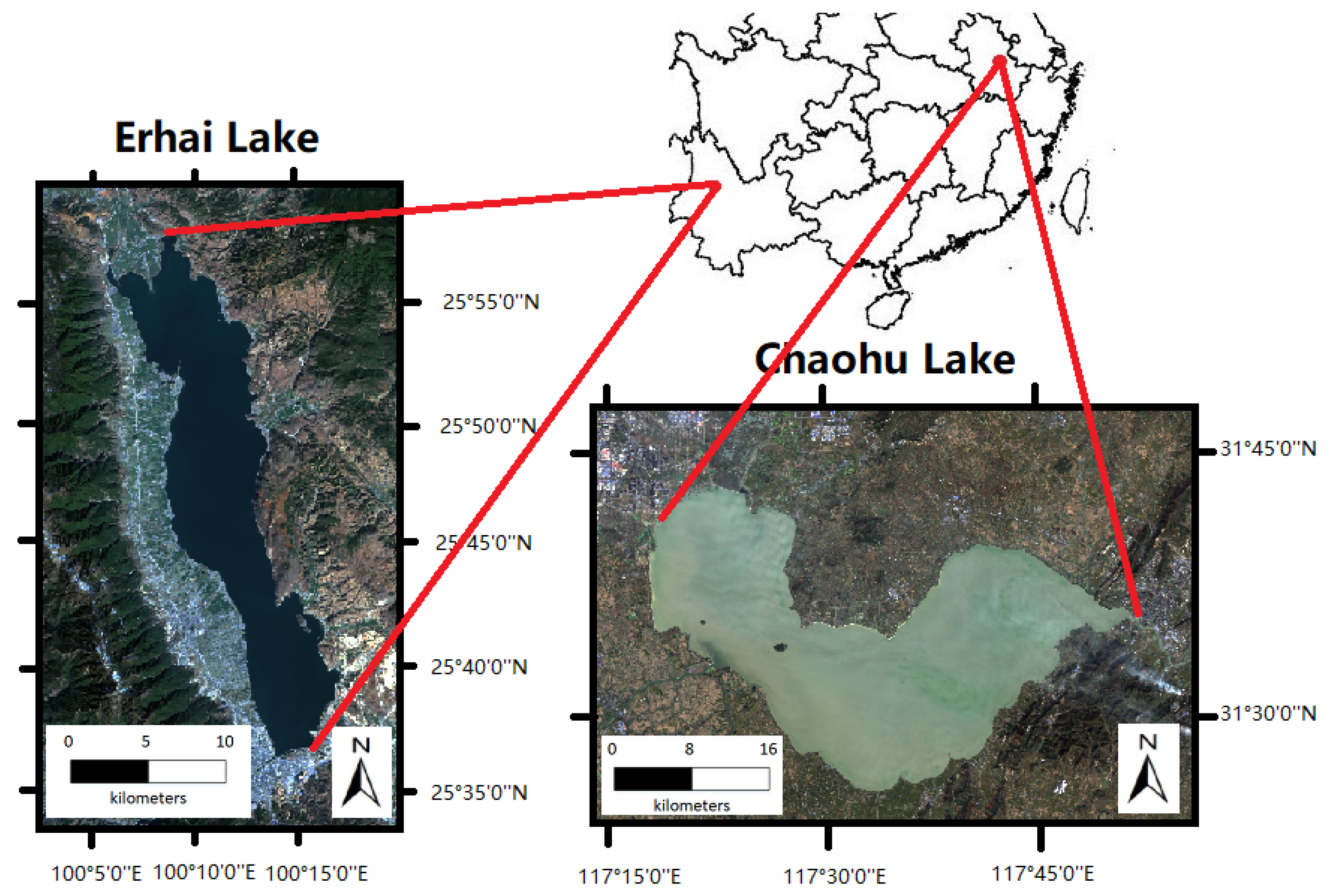
Erhai Lake and Chaohu Lake were used as the research areas for this study. Erhai Lake (2536 N–2558 N, 10006 E–10018 E), located in Dali, Yunnan Province, is a famous tourist spot in China. It has a water-surface area of 250 km, an average water depth of 10.5 m, and a maximum depth of 21 m. Fertilizer-rich agricultural runoffs and domestic sewage are discharged into Erhai, which increase TN and TP concentrations, and phytoplankton breeding. The water quality of Erhai Lake has deteriorated.
Chaohu Lake (3125 N–3143 N, 11716 E–11751 E), located in Hefei, Anhui Province, is one of China’s five major freshwater lakes. Chaohu Lake has a water surface area of 780 km, an average water depth of 2.89 m, and a maximum depth of 7.89 m. Unlike Dali, Hefei is one of the most developed cities in China. With rapid economic development, industrial and municipal wastewater has contributed to the pollution of Chaohu Lake. Chaohu Lake has been eutrophic since the 1980s. A large area of algal bloom broke out in 2015. Monitoring water quality is essential for eutrophication prevention in Erhai Lake and Chaohu Lake. The spatial locations of the two lakes are shown in Figure 1.
2.1.2. Satellite Data
Landsat8 Operational Land Imager (Landsat8 OLI) images were used for this study. Landsat8 was successfully launched by NASA on 11 February 2013. It is a sun-synchronous orbit satellite with an orbital altitude of 705 km, an orbital inclination of 98.2, and a time resolution of 16 days. Compared with the Enhanced Thematic Mapper Plus (ETM+) sensor mounted on Landsat7, Landsat8 OLI has two new bands, namely, the blue band (Band 1) and the short-wave infrared band (Band 9). Band 1 is mainly used for coastal observation, and Band 9 is usually used for cloud detection with water-vapor absorption characteristics. Landsat8 OLI has 9 bands with a wavelength ranging from 433 to 1390 nm, respectively. Band 8 is the full-color band with a spatial resolution of 15 m. Other bands have a spatial resolution of 30 m. Landsat8 OLI images can be freely downloaded from the website of the United States Geological Survey (USGS) (http://earthexplorer.usgs.gov).
Eighty-one images of Landsat8 OLI from January 2014 to October 2018 were collected for this study. To ensure the clarity of images, images with little cloud over the water area were selected. There are 41 images of Erhai Lake, Yunnan Province, and 40 images of Chaohu Lake, Anhui Province. The date range of the images corresponds to that of the in situ water-quality data.
2.1.3. In Situ Water-Quality Levels
The in situ water-quality data were collected from the official websites. Every week, the China National Environmental Monitoring Center (CNEMC) releases water-quality parameters (http://www.cnemc.cn/sssj/szzdjczb/) that are measured at national river cross-sections and monitoring sites. CNEMC also releases water-quality levels that are computed in terms of the observed water-quality parameters according to the GB3838-2002 standard. Water-quality parameters and water-quality levels are not only obtained at the established national observation sites, but also at monitoring sites deployed by the local governments.
The water-quality levels of Chaohu Lake from January 2014 to October 2018 were mainly collected from the website of CNEMC. The data come from two national cross-sections, the lake inlet at Hefei and the lake inlet at Yuxikou, respectively. Table 1 shows the downloaded water-quality parameters and levels of Chaohu Lake. For example, the water-quality level at Yuxikou station was computed as Class II in terms of GB3838-2002.
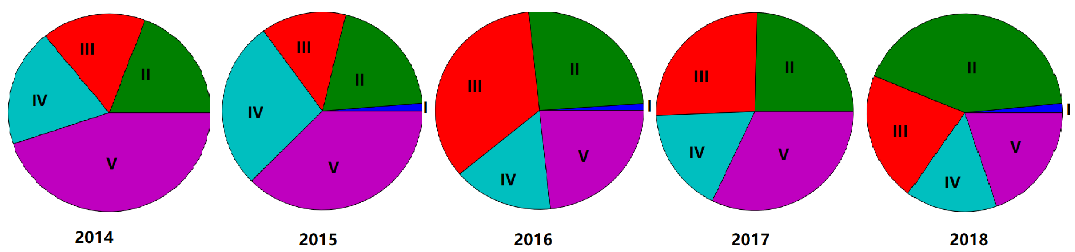
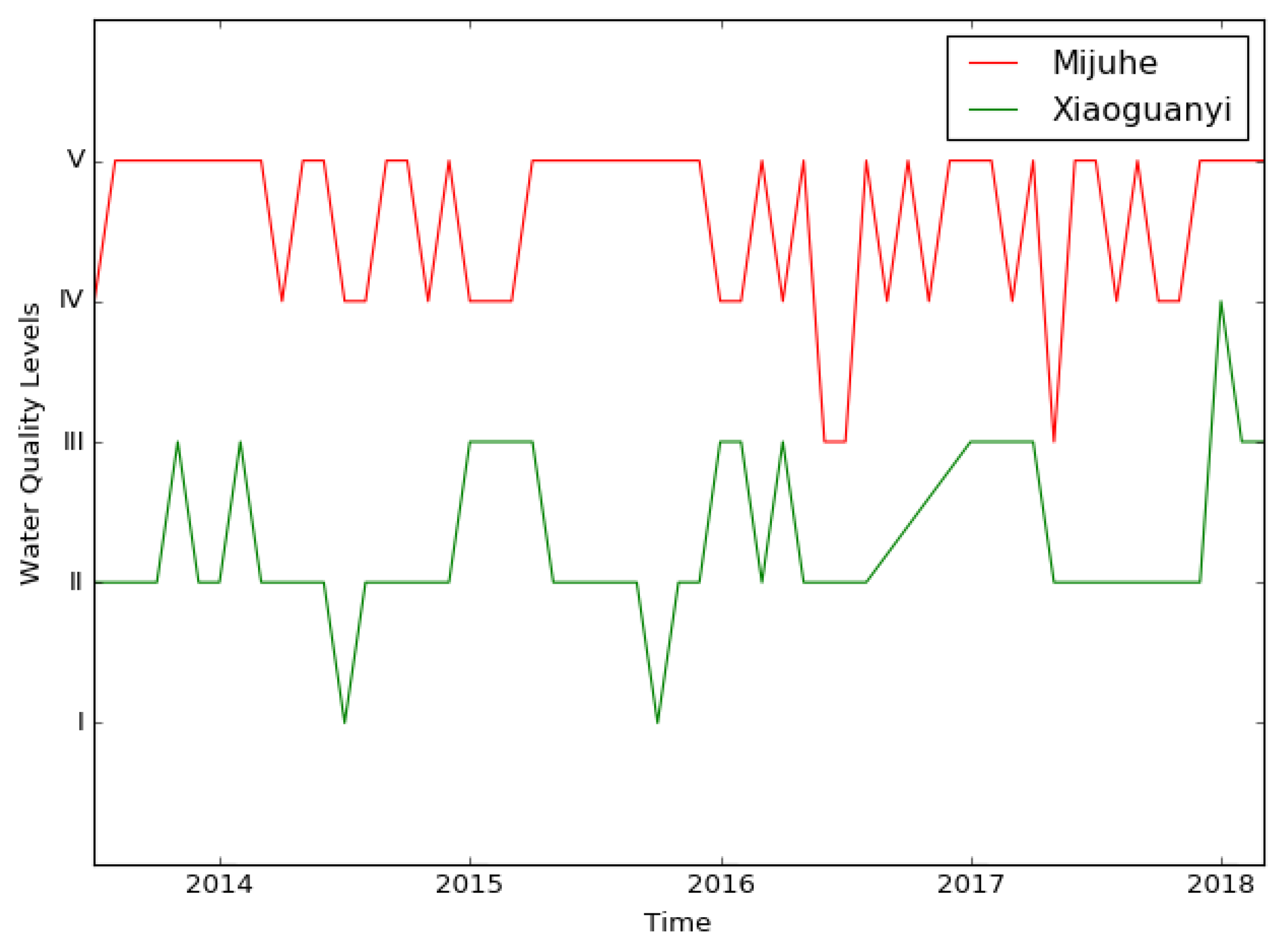
The water-quality levels of Erhai Lake from January 2014 to October 2018 were collected from the websites of both CNEMC and the Dali Bai Autonomous Prefecture Environmental Protection Agency (http://www.daliepb.gov.cn/hjzl/yuebao/). The data with a one-week cycle interval come from 2 national river cross-sections, and the data with a one-month cycle interval come from 8 local river cross-sections that were deployed at the 8 main-branch lake inlets. Table 2 shows the water-quality levels of Erhai Lake. Water-quality levels were released by Dali Bai Autonomous Prefecture Environmental Protection Agency. Major overstandard factors that determine water-quality levels in China are mainly nonoptically active parameters, as shown in Table 2. Water-quality levels of 10 monitoring stations at Erhai Lake are the basic data for our study. The fan-diagram distributions of water-quality levels from 2014 to 2018 are shown in Figure 2. The monthly changes of water-quality levels at 2 monitoring stations, Mijuhe and Xiaoguanyi, are shown, respectively, in Figure 3.
2.2. Methods
The multispectral data acquired by the satellite sensors are influenced by atmospheric absorption and scattering, sensor target illumination geometry, and the influence of climate changes. Therefore, remote-sensing images must to be preprocessed before they are used for water-quality classification. Location and scattering errors were eliminated through radiometric calibration and atmospheric correction. Remote-sensing images and in situ water-quality levels were matched spatially and temporarily with the transit satellite. Then, a suitable convolutional neural network was designed according to the dataset for water-quality classification.
2.2.1. Remote-Sensing Image Preprocessing
Radiometric calibration and atmospheric correction are important preprocessing steps in many remote-sensing fields [21,22,23]. Radiometric calibration is the process of converting the digital number (DN) of multidate satellite images to a reference image, band by band, with the aim of reducing sensor errors. Atmospheric correction is to retrieve accurate radiance and eliminate errors caused by atmospheric scattering, reflection, and absorption. Atmospheric correction models such as MODTRAN, LOWTRAN, and 6S are widely used. The MODTRAN code can solve the radiation transfer function through generating the physical parameters of atmospheric correction [24]. The fast line-of-sight atmospheric analysis of the spectral hypercube (FLAASH) atmospheric correction method incorporates the MODTRAN 4 radiation transfer code. FLAASH can eliminate the effect caused by the atmosphere and convert spectral radiance to water-surface reflectance [25,26,27]. Radiometric calibration and FLAASH atmospheric correction were processed by ENVI image-processing software.
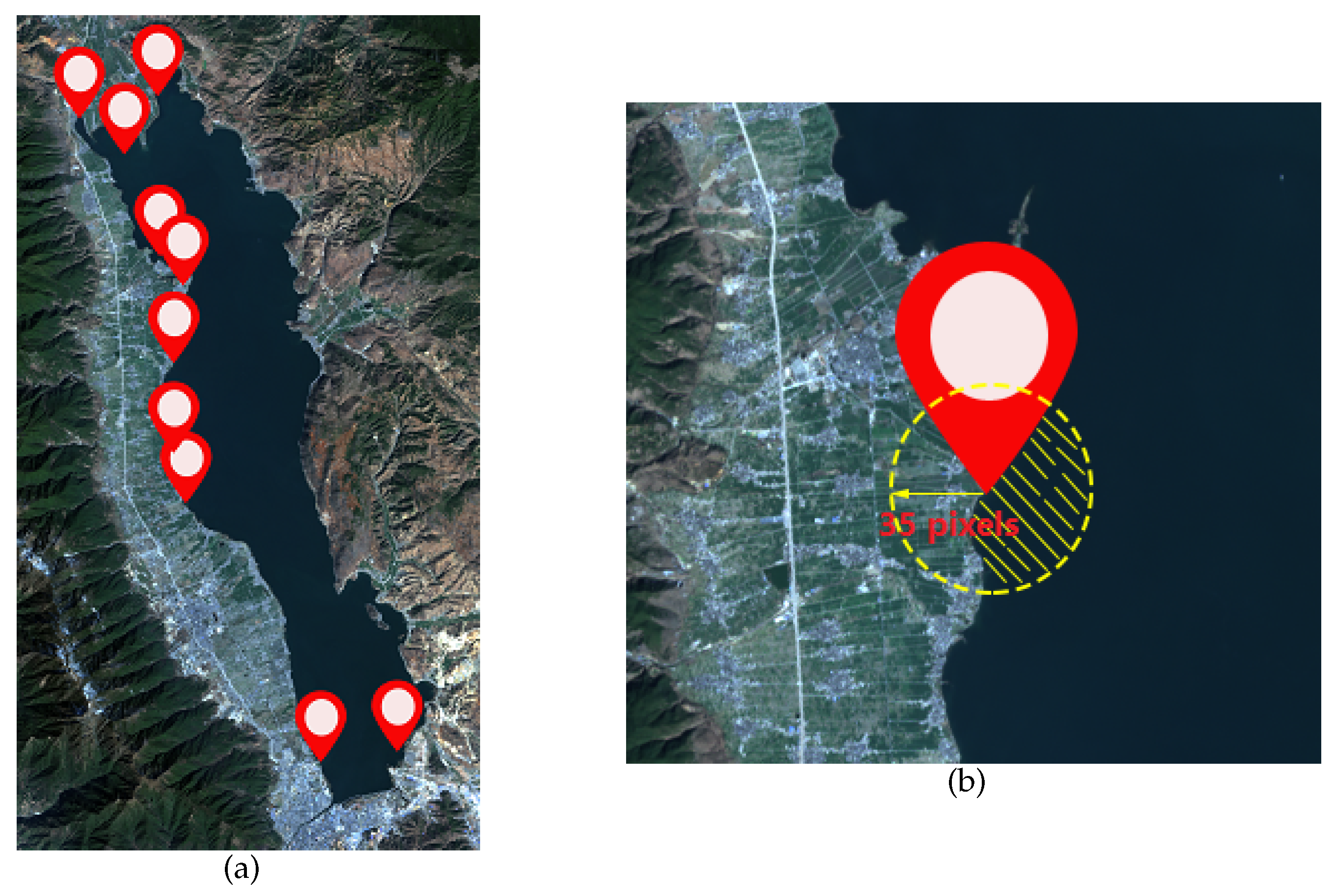
Because remote-sensing images and in situ water-quality levels are asynchronously acquired, images and in situ values should be matched in terms of time and geolocation before training and classification. Spatial matching is to find remote-sensing pixels that correspond to the geolocation of the in situ monitoring station. Temporal matching is to make in situ water-quality levels and remote-sensing images synchronous through selecting in situ data in the same month with the transit satellite. For example, there are 10 in situ monitoring stations in Erhai Lake, as shown in Figure 4a. The resolution of the Landsat8 images is 30 × 30 m, which means each pixel represents a 30 × 30 m area. The circular area with the radius of 1 km (about 35 pixels) was selected as the coverage of each monitoring station, as shown in Figure 4b. The samples containing land pixels were removed. We assumed that the water-quality levels of each pixel in the selected circle were the same as the water-quality levels observed by the in situ monitoring station. Our test results showed that the radius of the circle around each monitoring station had no significant effects on water-quality-level classification. After preprocessing, windows of 21 × 21 pixels around the centered pixels in each selected circle from Band 1 to 7 were chosen as the CNN training inputs.
2.2.2. Water-Quality-Level Classification Based on Convolutional Neural Networks
Convolutional neural networks have received a research boom in recent years, and have shown impressive performance in remote-sensing image processing [28,29]. Compared with SAEs and DBNs, CNN models have no requirement that input vectors must be one-dimension (1D) [19]. CNNs can learn discriminative and hierarchical features from multispectral data. AlexNet, which was developed by Krizhevsky, Sutskever, and Hinton [30], is viewed as the beginning of deep learning. AlexNet was the winning entry in ILSVRC 2012, and can learn both shallow and deep features. Optimization strategies such as overlapping sampling and nonlinear ReLU activation functions contribute to its classification performance. The structure of the AlexNet model is simpler than that of other CNN models such as VGG [31] and ResNet [32]. AlexNet is effective for small-size inputs.
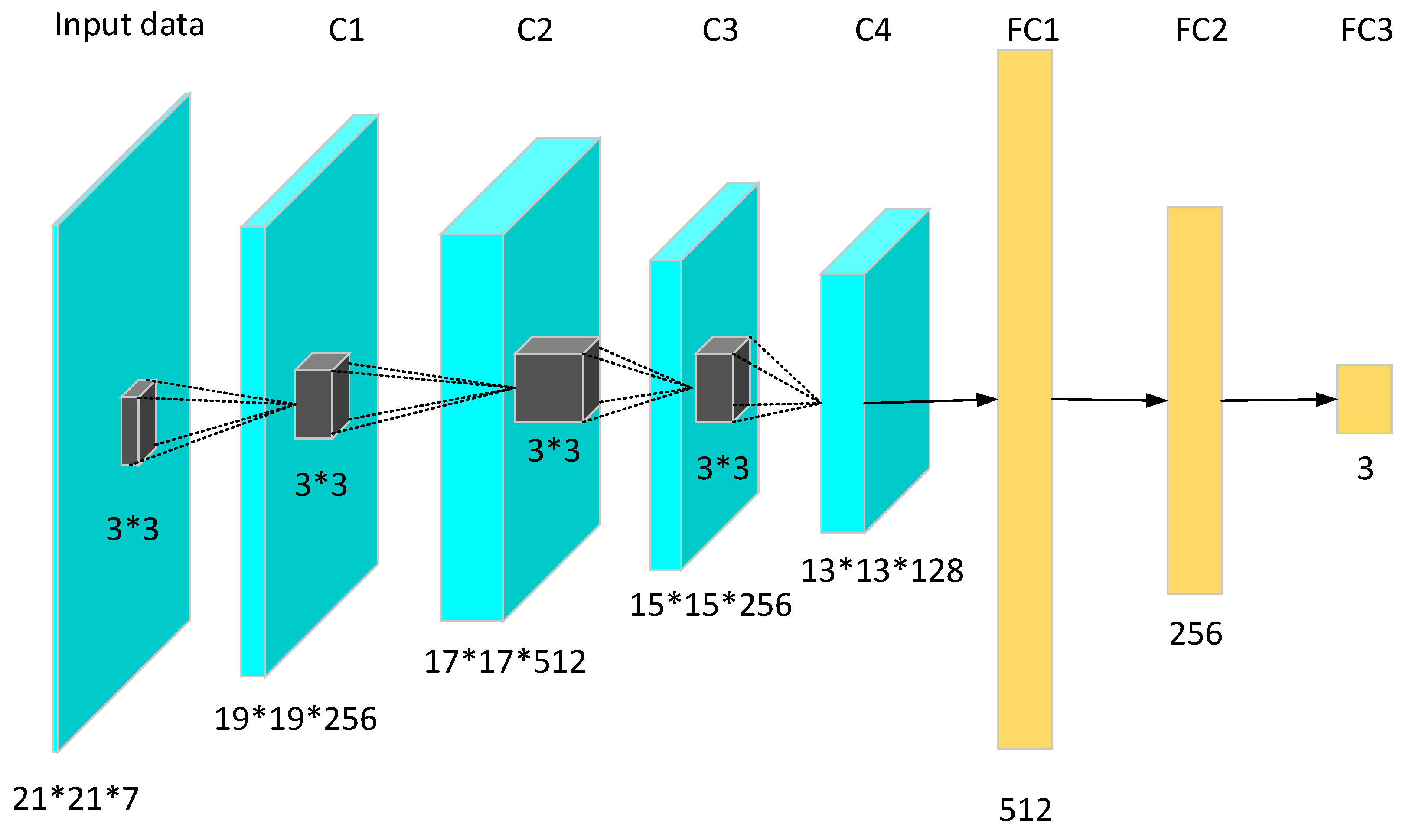
The structure of the convolutional neural network used for water-quality-level classification was designed as follow: (1) Considering a small input size of 21 × 21 × 7 pixels, the number of convolutional layers cannot be large. If the number of convolutional layers increases, the computational complexity of the CNN increases correspondingly. The best number of convolutional layers, from 2 to 7, is determined through testing water-quality classification. (2) Kernel sizes and the stride are set to be small. Zeiler et al. [33] found that reducing the kernel sizes and the stride of the AlexNet model could achieve better performance. (3) Pooling layers are removed in order to reserve information.
There were other settings: a Rectified Linear Unit (ReLU) was applied as the activation function of each layer. Three fully connected layers were also set behind convolutional layers, same as the AlexNet model. To balance the amount of each water-quality level, the output of the last fully connected layer was fed into a 3-way softmax layer that corresponded to 3 water-quality class labels: Class A, Class B, and Class C. Class A that includes Class I and Class II of the standard GB3838-2002 means good water quality. Class B, corresponding to Class III of the standard GB3838-2002, means water is used for fisheries and industry. Class C that covers Class IV, V, and above means water is not suitable for drinking and can be used for recreation and irrigation. A dropout technique was utilized between fully connected layers. The dropout technique randomly drops units along with their connections in order to prevent the CNN from overfitting [34].The architecture with 4 convolutional layers and 3 fully connected layers is shown in Figure 5.
2.2.3. Transfer Learning
If there is a small number of labelled data in a target task, it is hard to directly train a good CNN model. The problem can be solved by transfer learning. Transfer learning is a method using knowledge learned from source tasks to improve the performance of the target tasks without overfitting [35]. It avoids the random initialization of model weights for training, and also saves time. It is especially efficient for a deep architecture [36].
Considering that the number of in situ data of Chaohu Lake is less than that of Erhai Lake, transfer learning with the CNN model trained in Erhai Lake was applied to classify the water-quality level of Chaohu Lake. The model trained in Erhai Lake was transferred, and weights were fine-tuned to fit the data of Chaohu Lake. The experiment results demonstrate the effectiveness and robustness of our CNN model.
3. Results
The multispectral remote-sensing images were classified into three water-quality levels based on the designed CNN. The training samples for CNN were selected from 41 frames of Landsat8 images from January 2014 to October 2018 at Erhai Lake. The ratio of the training set to the test set was 4:1. Each convolutional layer had 128, 256, or 512 kernels. Kernel size was 3 × 3, and stride was set to 1. The number of kernels in three full connected layers was set to 512, 256, and 3 respectively, and the dropout strategy behind the first two fully connected layers was set to 50%. The CNN was trained by stochastic gradient descent with momentum. Training epochs were set to 1000, learning rate was set to , and momentum was set to 0.9.
Classification performance of the model was evaluated by overall accuracy (OA), which refers to the percentage of the correct number of samples to the total number of samples. We configured the CNN with a different number of convolution layers, from two to seven, respectively. Each configuration was tested five times on the Erhai Lake dataset. The classification results by the different number of convolutional layers are shown in Table 3. The CNN with four convolutional layers obtained the best results, and performances from three to seven convolutional layers did not largely vary. We configured our CNN with four convolutional layers as a tradeoff between accuracy and computing complexity.
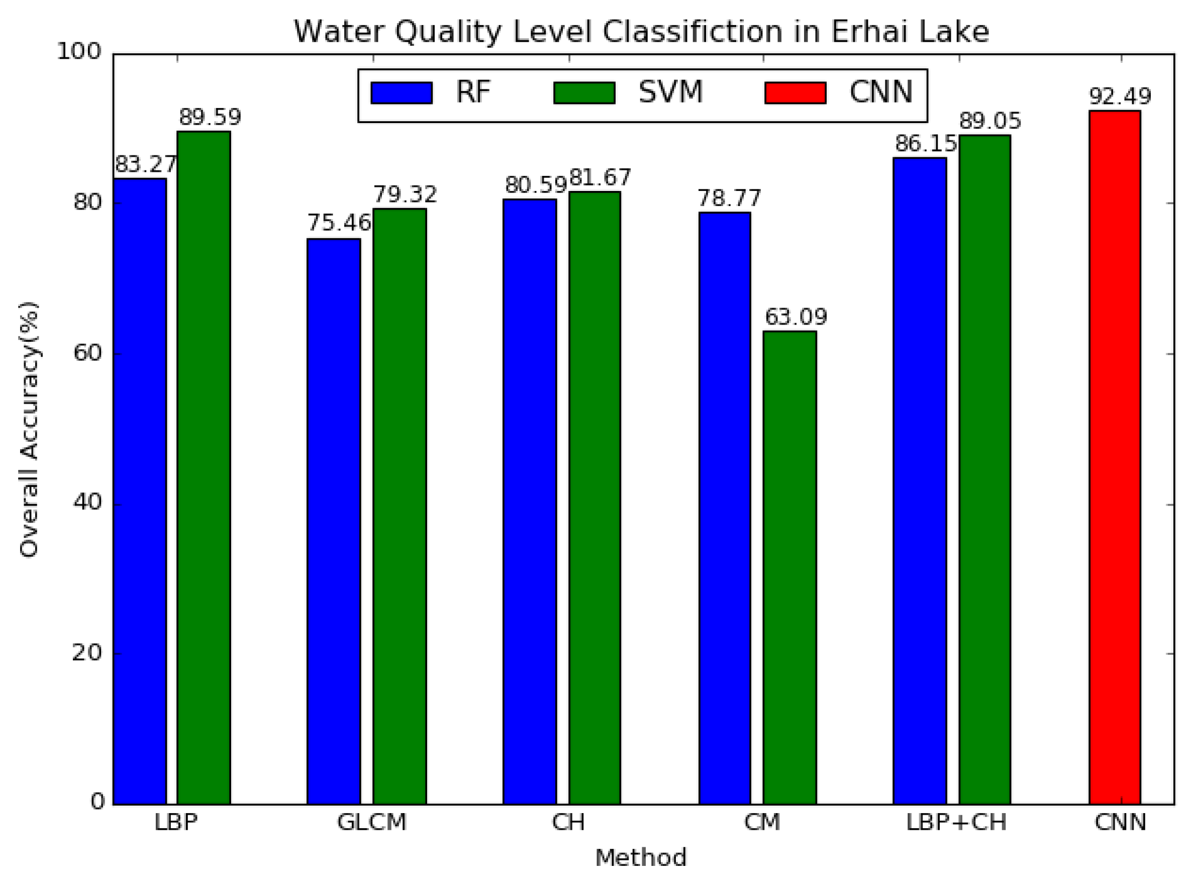
To evaluate CNN performance, we compared its classification performance with that of common machine-learning models SVM and RF. Visual features, such as texture and color features, were selected for classification. Local binary pattern (LBP) [37], gray level co-occurrence matrix (GLCM) [38], color histograms (CH), and color moments (CM) were the selected features for both SVM and RF.
Classification results in terms of OA are shown in Figure 6. Figure 6 indicates that CNN achieved the best classification performance, higher than the SVM-based and the RF-based methods. Combined features with LBP and CH were also tested, but classification accuracy was lower than the CNN method. The CNN was the best of all water-quality classification methods of Erhai Lake. Because of the powerful learning ability, the CNN can not only learn shallow features such as color and texture features, but also learn discriminative and complex features from multispectral images. Therefore, the CNN achieved the best classification performance.
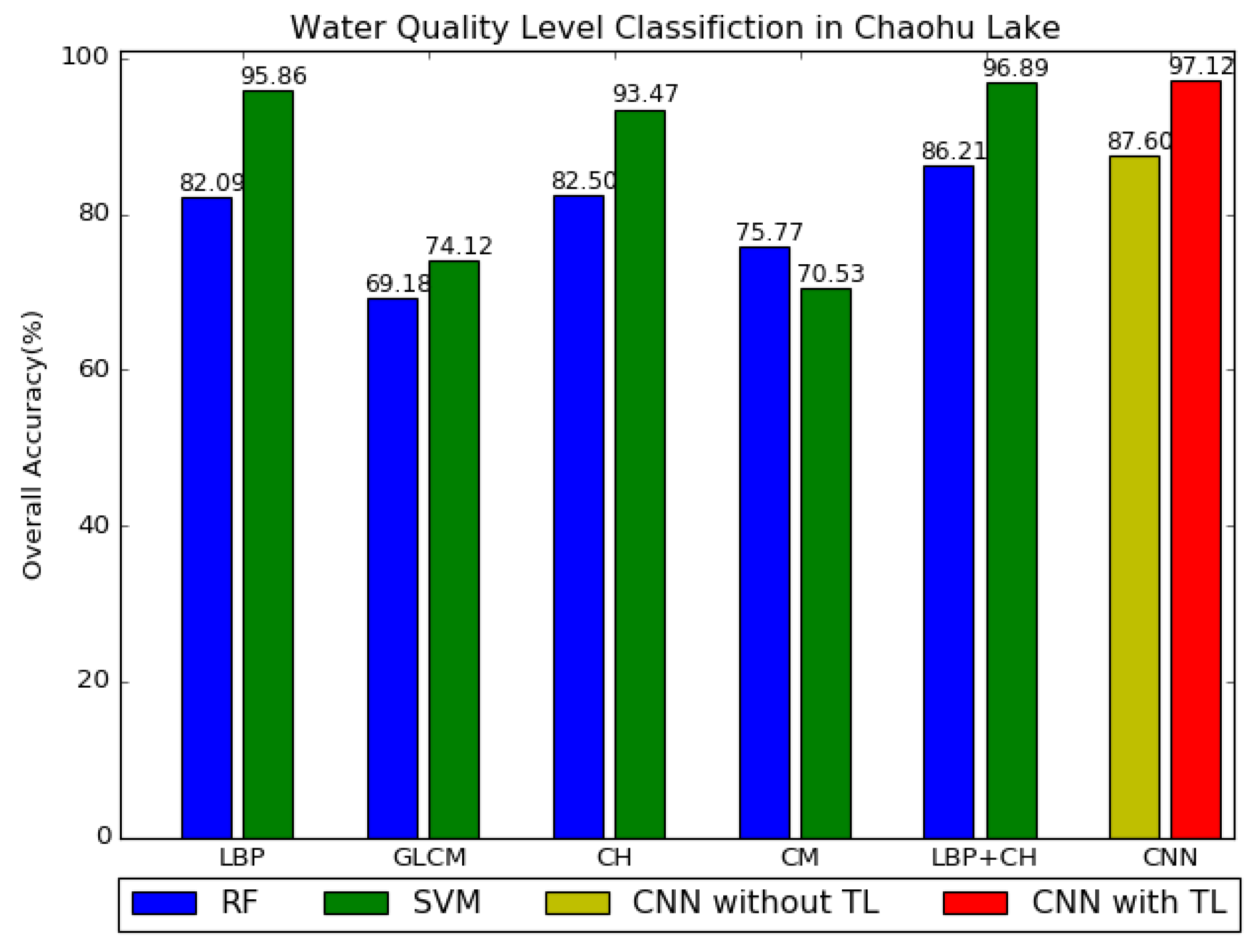
To test the model’s robustness, we conducted an additional experiment using 40 frames of Landsat8 images and in situ water-quality levels from January 2014 to October 2018 in Chaohu Lake. A transfer-learning experiment was conducted. The model trained in Erhai Lake was transferred to Chaohu Lake. Ten percent of samples at Chaohu Lake were used to finetune the CNN model. Classification results in terms of OA are shown in Figure 7.
The CNN models trained without transfer learning, and the traditional algorithms using SVM or RF were also tested in Chaohu Lake. The results are also listed in Figure 7. Because only 10% of samples were used for training, the CNN model without transfer learning was overfitting, causing low classification accuracy. The transferred CNN models achieved the best classification performance.
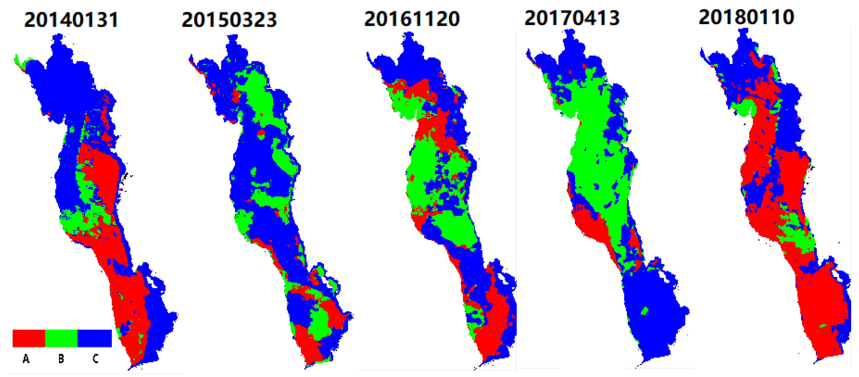
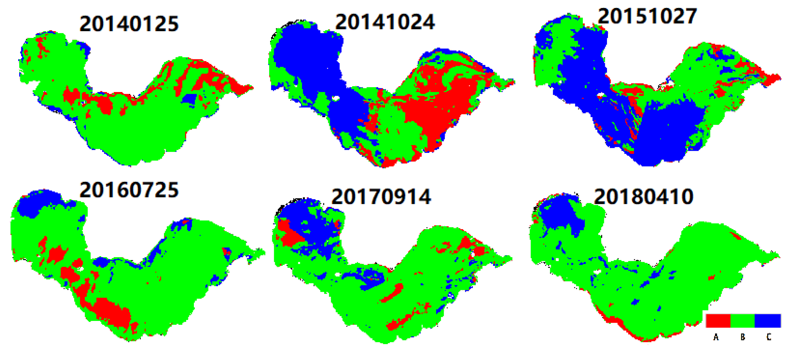
Water-quality classification of the whole body in Erhai Lake and Chaohu Lake in five years is shown in Figure 8 and Figure 9, respectively. As shown in Figure 8, the worst pollution area of Erhai Lake is on the northern part. In Chaohu Lake, the worst pollution area is on the western part, and a large area of the water region was polluted on 27 October 2015, which is shown in Figure 9.
Both experiments demonstrate that the CNN is powerful in the extraction of the relationship between the Landsat8 images and water-quality levels. Application of the CNN to remotely sense water-quality levels provides a cost-effective mode for water-quality monitoring of the whole water body.
4. Discussion
Water quality is strongly related with population and land use along the lakes. Results demonstrate the efficiency of our models. Two main inflows are located in the north of Erhai Lake. Agriculture and domestic sewage deteriorate the water quality of the northern Erhai Lake. In Figure 8, we can see that the worst water-quality regions are in the north. The result is consistent with conclusions in previous studies [11]. Besides, in [11], the Chl-a concentration map on 12 November 2016 is similar to the water-quality-level distribution on 20 November 2016, shown in Figure 8. Although the water-quality levels of GB3838-2002 are not directly dependent on Chl-a according to Appendix A, nonoptically active parameters such as TN and TP are closely related to Chl-a and other optically active parameters [3,5]. Hefei, the provincial capital of Anhui Province, is located in the western part of Chaohu Lake. With the rapid development of the economy and the growth of population in Hefei, domestic and industrial wastewater contribute to the pollution of western Chaohu Lake. The results in Figure 9 also have similar conclusions to [5]. A large area of algal blooms also broke out in 2015, and bloom coverage was more than 40% of the whole lake. The blooms lasted until 2016. The classification results of Chaohu Lake on 27 October 2015 are also presented in Figure 9. Water quality was almost contaminated in that period. All analyses demonstrate that the classification results are verifiable.
Many scholars have proposed a variety of methods for water-quality monitoring [4,6,7,8,9], and some studies were used for Erhai Lake and Chaohu Lake [5,11,39,40]. These methods mainly focus on a single water-quality parameter, such as Chl-a or TP. Some conclusions of these studies are consistent with our results. However, as mentioned in [5], remote-sensing reflectance is influenced by many water-quality variables, such as Chl-a, TSS, and CDOM, rather than a single parameter. As shown in Table 2, major overstandard factors that determine water-quality levels are often more than one parameter. In this paper, water-quality level is a systematic index for water-quality assessment. Water-quality classification based on water-quality levels can eliminate errors caused by a single parameter. So, using water-quality levels for water-quality monitoring and management is more suitable and effective.
Some results of water-quality classification are not well-correlated with in situ water-quality levels. The reasons involve two main aspects: First, the interval between in situ sampling dates and imaging dates may cause errors. As shown in Figure 6 and Figure 7, classification accuracy in Chaohu Lake is better than that in Erhai Lake because of a shorter time interval between remote-sensing images and in situ measurements. Another reason is weather. In rainy days, nutrients flow into the lakes and water may be turbid. Concentrations of water-quality parameters also vary with the influence of wind. Clouds may also affect satellite imaging. Therefore, climate change and weather conditions may also cause errors in water-quality classification.
Experiment results show that the CNN was powerful in water-quality classification. CNN performance is mainly related to factors such as the number of convolutional layers and training samples that were analyzed in this section. CNN accuracy varies with the number of convolutional layers. Accuracy may increase with the increase of the number of convolutional layers. However, when the number of convolutional layers is greater than five, CNN performance drops. The reason may be that details of small inputs disappear. There may exist an optimal number of convolutional layers. Accuracy is also affected by the number of training samples. In the experiment at Chaohu Lake, using 10% of samples to train a CNN model caused low classification accuracy. The reason was overfitting. This problem can be solved and classification performance can be improved by a transfer-learning strategy. The experiment results demonstrate that a transfer-learning strategy is available for water-quality classification of inland lakes in China. In addition, the performance of the transferred CNN in Chaohu Lake was better than that of the basic CNN model, which illustrates that CNN weight initialization is important.
Our work provides an accurate and cost-effective method to monitor water quality. In the future, we will use water-quality-related variables to improve classification performance and interpret the CNN model for water-quality assessment.
5. Conclusions
In this paper, we configured a convolutional neural network in terms of AlexNet to model the relationship between Landsat8 images and in situ water-quality levels. The CNN consisted of four convolutional layers and three fully connected layers. We trained the CNN model at Erhai Lake using spatially and temporarily matched Landsat8 images, and in situ monitoring data. Compared with traditional machine-learning methods SVM and RF, CNN had the best classification accuracy. Another advantage of CNN is its transfer learning. The model trained at Erhai Lake could be applied for water-quality classification at Chaohu Lake. Our works indicates that the configured CNN can be used to monitor the water quality of inland lakes through remote-sensing images. Our method provides a cost-effective way to enlarge spatial-monitoring coverage. It improves both the accuracy and coverage of inland-lake monitoring. Our future work will focus on improving the interpretability of CNN models using water-quality-related variables.
Author Contributions
F.P. contributed the idea and guided the whole work. C.D. designed the CNN and made the software. Z.C. spatially and temporarily matched the remote-sensing images and in situ data. Y.Y. contributed to the image preprocessing. X.X. helped to design the CNN. All authors contributed to the writing of the paper.
Funding
This research received no external funding.
Acknowledgments
This work was supported by the National Key Research and Development Program of China (No. 2016YFB0502600). It was also supported by the Thirteen-Five Civil Aerospace Planning Project—Integration of Communication, Navigation, and Remote Sensing Comprehensive Application Technology.
Conflicts of Interest
No conflict of interest.
Abbreviations
The following abbreviations are used in this manuscript:
| CNN | Convolutional neural network |
| Chl-a | Chlorophyll-a |
| TSS | Turbidity and Suspended solids |
| CODM | Colored dissolved organic matter |
| TN | Total nitrogen |
| TP | Total phosphorus |
| COD | Chemical oxygen demand |
| DO | Dissolved oxygen |
| DL | Deep learning |
| SVM | Support vector machine |
| RF | Random forest |
| SAE | Stacked autoencoder |
| DBN | Deep-belief network |
| Landsat8 OLI | Landsat8 Operational Land Imager |
| ETM+ | Enhanced Thematic Mapper Plus |
| USGS | United States Geological Survey |
| CNEMC | China National Environmental Monitoring Center |
| FLAASH | Fast line-of-sight atmospheric analysis of spectral hypercube |
| ReLU | Rectified Linear Unit |
| OA | Overall accuracy |
| TL | Transfer learning |
| LBP | Local binary pattern |
| GLCM | Gray level co-occurrence matrix |
| CH | Color histograms |
| CM | Color moments |
Appendix A
The classification standards of water quality according to GB3838-2002 in China are shown in Table A1. Five water-quality levels are in GB3838-2002. Higher water-quality levels represent worse water quality. Water quality is classified using a single-factor method, which means the parameter that exceeds its corresponding criterion with the highest proportion is selected for water-quality-level classification.

Table A1.
Classification standards of water-quality levels in GB3838-2002.
| Numbers | Parameters (Unit: mg/L) | Water-Qualtiy Levels | ||||
|---|---|---|---|---|---|---|
| I | II | III | IV | V | ||
| 1 | pH (No unit) | 6–9 | ||||
| 2 | DO | ≥7.5 | ≥6 | ≥5 | ≥3 | ≥2 |
| 3 | Permanganate | ≤2 | ≤4 | ≤6 | ≤10 | ≤15 |
| 4 | COD | ≤15 | ≤15 | ≤20 | ≤30 | ≤40 |
| 5 | BOD_5 | ≤3 | ≤3 | ≤4 | ≤6 | ≤10 |
| 6 | NH_3-N | ≤0.15 | ≤0.5 | ≤1 | ≤1.5 | ≤2 |
| 7 | TP | ≤0.02 | ≤0.1 | ≤0.2 | ≤0.3 | ≤0.4 |
| 8 | TN | ≤0.2 | ≤0.5 | ≤1 | ≤1.5 | ≤2 |
| 9 | Cu | ≤0.01 | ≤1 | ≤1 | ≤1 | ≤1 |
| 10 | Zn | ≤0.05 | ≤1 | ≤1 | ≤2 | ≤2 |
| 11 | Fluoride | ≤1 | ≤1 | ≤1 | ≤1.5 | ≤1.5 |
| 12 | Se | ≤0.01 | ≤0.01 | ≤0.01 | ≤0.02 | ≤0.02 |
| 13 | As | ≤0.05 | ≤0.05 | ≤0.05 | ≤0.1 | ≤0.1 |
| 14 | Hg | ≤0.00005 | ≤0.00005 | ≤0.0001 | ≤0.001 | ≤0.001 |
| 15 | Cd | ≤0.001 | ≤0.005 | ≤0.005 | ≤0.005 | ≤0.01 |
| 16 | Cr | ≤0.01 | ≤0.05 | ≤0.05 | ≤0.05 | ≤0.1 |
| 17 | Pb | ≤0.01 | ≤0.01 | ≤0.05 | ≤0.05 | ≤0.1 |
| 18 | Cyanide | ≤0.005 | ≤0.05 | ≤0.2 | ≤0.2 | ≤0.2 |
| 19 | Volatile phenol | ≤0.002 | ≤0.002 | ≤0.005 | ≤0.01 | ≤0.1 |
| 20 | Petroleum | ≤0.05 | ≤0.05 | ≤0.05 | ≤0.5 | ≤1 |
| 21 | Anionic surfactant | ≤0.2 | ≤0.2 | ≤0.2 | ≤0.2 | ≤0.3 |
| 22 | Sulfide | ≤0.05 | ≤0.1 | ≤0.2 | ≤0.5 | ≤1 |
| 23 | Fecal coliform | ≤200 | ≤2000 | ≤10,000 | ≤20,000 | ≤40,000 |
References
- Su, J.; Ji, D.F.; Mao, L.; Chen, Y.Q.; Sun, Y.Y.; Huo, S.L.; Zhu, J.C.; Xi, B.D. Developing surface water quality standards in China. Resour. Conserv. Recycl. 2016, 117, 294–303. [Google Scholar] [CrossRef]
- Chen, K.; Ni, M.; Cai, M.; Wang, J.; Huang, D.; Chen, H.; Wang, X.; Liu, M. Optimization of a coastal environmental monitoring network based on the Kriging method: A case study of quanzhou cay, China. BioMed Res. Int. 2016, 1, 1–12. [Google Scholar] [CrossRef]
- Hajigholizadeh, M.; Melesse, A.M.; Reddi, L. A comprehensive review on water quality parameters estimation using remote sensing techniques. Sensors 2016, 16, 1298. [Google Scholar] [CrossRef] [PubMed]
- Nazeer, M.; Bilal, M.; Alsahli, M.M.M.; Shahzad, M.I.; Waqas, A. Evaluation of empirical and machine learning algorithms for estimation of coastal water quality parameters. Int. J. Geo-Inf. 2017, 6, 360. [Google Scholar] [CrossRef]
- Du, C.; Wang, Q.; Li, Y.; Lyu, H.; Zhu, L.; Zheng, Z.; Wen, S.; Liu, G.; Guo, Y. Estimation of total phosphorus concentration using a water classification method in inland water. Int. J. Appl. Earth Obs. Geoinf. 2018, 71, 29–42. [Google Scholar] [CrossRef]
- Yu, X.; Yi, H.; Liu, X.; Wang, Y.; Liu, X.; Zhang, H. Remote-sensing estimation of dissolved inorganic nitrogen concentration in the Bohai Sea using band combinations derived from MODIS data. Int. J. Remote Sens. 2017, 37, 327–340. [Google Scholar] [CrossRef]
- Singh, A.; Jakubowski, A.; Chidister, I.; Townsend, P.A. A MODIS approach to predicting stream water quality in Wisconsin. Remote Sens. Environ. 2013, 128, 74–86. [Google Scholar] [CrossRef]
- Mathew, M.M.; Rao, N.S.; Mandla, V.R. Development of regression equation to study the total nitrogen, total phosphorus and suspended sediment using remote sensing data in Gujarat and Maharashtra coast of India. J. Coastal Conserv. 2017, 21, 1–11. [Google Scholar] [CrossRef]
- Politi, E.; Prairie, Y.T. The potential of earth observation in modelling nutrient loading and water quality in lakes of southern Québec, Canada. Aquat. Sci. 2018, 80, 8. [Google Scholar] [CrossRef]
- Politi, E.; Cutler, M.E.J.; Rowan, J.S. Evaluating the spatial transferability and temporal repeatability of remote-sensing-based lake water quality retrieval algorithms at the European scale: A meta-analysis approach. Aquat. Sci. 2015, 36, 3005. [Google Scholar] [CrossRef]
- Tan, W.X.; Liu, P.C.; Liu, Y.; Yang, S.; Feng, S. A 30-year assessment of phytoplankton blooms in Erhai Lake using Landsat imagery: 1987 to 2016. Remote Sens. 2017, 12, 1265. [Google Scholar] [CrossRef]
- Min, C.; Ning, W.; Li, F. Extraction of water body with different water quality types based on Landsat8 image. J. Anhui Agric. Sci. 2016, 30, 220–222. [Google Scholar]
- Kuang, R.Y.; Luo, W.; Zhang, M. Optical classification of Poyang Lake waters based on in situ measurements and remote sensing images. Resour. Environ. Yangtze Basin 2015, 5, 1. [Google Scholar]
- Vapnik, V.V. The nature of statistical learning theory. In The Nature of Statistical Learning Theory; Springer: Berlin, Germany, 2000. [Google Scholar]
- Zhou, Y.; Chen, Y.H.; Feng, L.; Zhang, X.; Shen, Z.F.; Zhou, X.C. Supervised and adaptive feature weighting for object-based classification on satellite images. IEEE J. Sel. Top. Appl. Earth Obs. Remote Sens. 2018, 99, 1–11. [Google Scholar] [CrossRef]
- Cutler, A.; Cutler, D.R.; Stevens, J.R. Random forests. Mach. Learn. 2011, 45, 157–176. [Google Scholar]
- Tong, X.Y.; Lu, Q.K.; Xia, G.S.; Zhang, L.P. Large-scale land cover classification in GaoFen-2 satellite imagery. In Proceedings of the IGARSS 2018—IEEE International Geoscience and Remote Sensing Symposium, Valencia, Spain, 22–27 July 2018. [Google Scholar]
- Zhang, L.P.; Zhang, L.F.; Du, B. Deep learning for eemote sensing data: A technical tutorial on the State of the art. IEEE Geosci. Remote Sens. Mag. 2016, 4, 22–40. [Google Scholar] [CrossRef]
- Haut, J.M.; Paoletti, M.E.; Plaza, J.; Li, J.; Plaza, A.; Chen, H.; Wang, X.; Liu, M. Active learning with convolutional neural networks for hyperspectral image classification using a new Bayesian approach. IEEE Trans. Geosci. Remote Sens. 2018, 99, 1–22. [Google Scholar] [CrossRef]
- Zhao, W.; Jiao, L.C.; Ma, W.P.; Zhao, J.Q.; Zhao, J.; Liu, X.H.; Yang, S.Y. Superpixel-based multiple local CNN for panchromatic and multispectral image classification. IEEE Trans. Geosci. Remote Sens. 2017, 99, 1–16. [Google Scholar] [CrossRef]
- Brook, A.; Dor, E.B. Supervised vicarious calibration SVC of hyperspectral remote-sensing data. Remote Sens. Environ. 2011, 115, 1543–1555. [Google Scholar] [CrossRef]
- Lu, D.S.; Mausel, P.; Brondizio, E.S.; Moran, E. Assessment of atmospheric correction methods for Landsat TM data applicable to Amazon basin LBA research. Int. J. Remote Sens. 2002, 23, 2651–2671. [Google Scholar] [CrossRef]
- Nazeer, M.; Nichol, J. Improved water quality retrieval by identifying optically unique water classes. J. Hydrol. 2016, 541, 1119–1132. [Google Scholar] [CrossRef]
- Pyo, J.; Ligaray, M.; Kwon, Y.S.; Ahn, M.H.; Kim, K.; Lee, H.; Kang, T.; Cho, S.B.; Park, Y.; Cho, K.H. High-spatial resolution monitoring of phycocyanin and chlorophyll-a using airborne hyperspectral imagery. Remote Sens. 2018, 10, 1180. [Google Scholar] [CrossRef]
- Liu, J.M.; Zhang, Y.J.; Yuan, D.; Song, X.Y. Empirical estimation of total nitrogen and total phosphorus concentration of urban water bodies in china using high resolution IKONOS multispectral imagery. Water 2015, 7, 6551–6573. [Google Scholar] [CrossRef]
- Xu, X.; Huang, X.L.; Zhang, Y.L.; Yu, D. Long-term changes in water clarity in lake Liangzi determined by remote sensing. Remote Sens. 2018, 10, 1441. [Google Scholar] [CrossRef]
- Liu, D.Z.; Fu, D.Y. Atmospheric correction of Hyperion imagery over estuarine waters: A case study of the Pearl River Estuary in southern China. Int. J. Remote Sens. 2017, 38, 199–210. [Google Scholar] [CrossRef]
- Souleyman, C.; Liu, H.; Gu, Y.F.; Yao, H.X. Deep feature fusion for VHR remote sensing scene classification. IEEE Trans. Geosci. Remote Sens. 2017, 99, 1–10. [Google Scholar]
- Cheng, G.; Yang, C.Y.; Yao, X.W.; Li, K.M.; Han, J.W. When deep learning meets metric learning: Remote sensing image scene classification via learning discriminative CNNs. IEEE Trans. Geosci. Remote Sens. 2018, 99, 1–11. [Google Scholar] [CrossRef]
- Krizhevsky, A.; Sutskever, I.; Hinton, G. ImageNet Classification with Deep Convolutional Neural Networks; NIPS Curran Associates, Inc.: Harrahs and Harveys, Lake Taho, NV, USA, 2012. [Google Scholar]
- Simonyan, K.; Zisserman, M. Very deep convolutional networks for large-scale image recognition. arXiv 2014, arXiv:1409.1556. [Google Scholar]
- He, K.M.; Zhang, X.Y.; Ren, S.Q.; Sun, J. Deep residual learning for image recognition. In Proceedings of the 2016 IEEE Conference on Computer Vision and Pattern Recognition (CVPR), Las Vegas, NV, USA, 27–30 June 2016. [Google Scholar]
- Zeiler, M.D.; Fergus, R. Visualizing and understanding convolutional networks. In European Conference on Computer Vision; Springer: Cham, Switzerland, 2013. [Google Scholar]
- Srivastava, N.; Hinton, G.; Krizhevsky, A.; Sutskever, I.; Salakhutdinov, R. Dropout: A simple way to prevent neural networks from overfitting. J. Mach. Learn. Res. 2014, 15, 1929–1958. [Google Scholar]
- Yosinski, J.; Clune, J.; Bengio, Y.; Lipson, H. How transferable are features in deep neural networks? arXiv 2014, arXiv:1411.1792. [Google Scholar]
- Saeed, A.; Khan, A.; Zameer, A.; Usman, A. Wind power prediction using deep neural network based meta regression and transfer learning. Appl. Soft Comput. 2017, 58, 742–755. [Google Scholar]
- Ojala, T.; Pietikainen, M.; Harwood, D. A comparative study of texture measures with classification based on feature distributions. Pattern Recognit. 1996, 29, 51–59. [Google Scholar] [CrossRef]
- Haralick, R.M.; Shanmugam, K.; Dinstein, I. Textural features for image classification. Stud. Media Commun. 1990, 3, 610–621. [Google Scholar] [CrossRef]
- Yu, G.L.; Yang, W.; Matsushita, B.; Li, R.H.; Oyama, Y.; Fukushima, T. Remote estimation of chlorophyll-a in inland waters by a NIR-red-based algorithm: Validation in Asian Lakes. Remote Sens. 2014, 4, 3492–3510. [Google Scholar] [CrossRef]
- Wu, L.; Wang, L.; Min, L.; Hou, W.; Guo, Z.W.; Zhao, J.H.; Li, N. Discrimination of algal-bloom using spaceborne SAR observations of Great Lakes in China. Remote Sens. 2018, 5, 767. [Google Scholar] [CrossRef]
Figure 1.
Spatial locations of study areas.

Figure 2.
Yearly distribution of water-quality levels using fan diagram on 10 monitoring stations in Erhai Lake.
Figure 2.
Yearly distribution of water-quality levels using fan diagram on 10 monitoring stations in Erhai Lake.

Figure 3.
Monthly change of water-quality levels at 2 monitoring stations.

Figure 4.
Monitoring stations’ location. (a) Ten monitoring stations’ location in Erhai Lake. (b) Coverage area of a station.
Figure 4.
Monitoring stations’ location. (a) Ten monitoring stations’ location in Erhai Lake. (b) Coverage area of a station.

Figure 5.
CNN model architecture with 4 convolutional layers.

Figure 6.
Comparisions of water-quality classification performance in Erhai Lake.

Figure 7.
Comparisions of water-quality classification performance in Chaohu Lake.

Figure 8.
Whole water-body classification in Erhai Lake from 2014 to 2018.

Figure 9.
Whole water-body classification in Chaohu Lake from 2014 to 2018.

Table 1.
Water-quality data of Chaohu Lake by the China National Environmental Monitoring Center, on the 22nd week of 2018.
Table 1.
Water-quality data of Chaohu Lake by the China National Environmental Monitoring Center, on the 22nd week of 2018.
| Water Body | Stations | Section | Assessment (mg/L) | Water-Quality | |||
|---|---|---|---|---|---|---|---|
| pH | DO | COD | NH | ||||
| Chaohu Lake | Hefei Hubin | Chaohu | 7.69 | 11.6 | 4.4 | 0.18 | III |
| Chaohu Yuxikou | East Lake | 7.63 | 10.5 | 3.0 | 0.21 | II | |
Table 2.
Water quality of Erhai Lake and its main streams, published by Dali Bai Autonomous Prefecture Environmental Protection Agency, in October 2018.
Table 2.
Water quality of Erhai Lake and its main streams, published by Dali Bai Autonomous Prefecture Environmental Protection Agency, in October 2018.
| Numbers | Streams | Location | Responsible Department | Water-Quality Level | Major Overstandard Factors |
|---|---|---|---|---|---|
| 1 | Mijuhe | Yinqiaocun | Eryuan county | IV | TP, TN |
| 2 | Mijuhe | Dafengluqiao | Eryuan county | V | TP, TN |
| 3 | Mijuhe | Lake inlet | Shangguan town | IV | TP, TN |
| 4 | Yong’anjiang | Lianhecun | Eryuan county | V | DO, TP, TN |
| 5 | Yong’anjiang | Xichangcun | Eryuan county | V | DO, TP, TN |
| 6 | Yong’anjiang | Lake inlet | Shangguan town | V | DO, TP, TN |
Table 3.
Average accuracy by the different number of convolutional layers in Erhai Lake.
| The Number of convolutional layers | 2 | 3 | 4 | 5 | 6 | 7 |
| Average accuracy | 89.90% | 92.26% | 92.49% | 92.40% | 92.10% | 92.09% |
© 2019 by the authors. Licensee MDPI, Basel, Switzerland. This article is an open access article distributed under the terms and conditions of the Creative Commons Attribution (CC BY) license (http://creativecommons.org/licenses/by/4.0/).
Share and Cite
MDPI and ACS Style
Pu, F.; Ding, C.; Chao, Z.; Yu, Y.; Xu, X. Water-Quality Classification of Inland Lakes Using Landsat8 Images by Convolutional Neural Networks. Remote Sens. 2019, 11, 1674. https://0-doi-org.brum.beds.ac.uk/10.3390/rs11141674
AMA Style
Pu F, Ding C, Chao Z, Yu Y, Xu X. Water-Quality Classification of Inland Lakes Using Landsat8 Images by Convolutional Neural Networks. Remote Sensing. 2019; 11(14):1674. https://0-doi-org.brum.beds.ac.uk/10.3390/rs11141674
Chicago/Turabian StylePu, Fangling, Chujiang Ding, Zeyi Chao, Yue Yu, and Xin Xu. 2019. "Water-Quality Classification of Inland Lakes Using Landsat8 Images by Convolutional Neural Networks" Remote Sensing 11, no. 14: 1674. https://0-doi-org.brum.beds.ac.uk/10.3390/rs11141674
Note that from the first issue of 2016, this journal uses article numbers instead of page numbers. See further details here.