Using Solar-Induced Chlorophyll Fluorescence Observed by OCO-2 to Predict Autumn Crop Production in China

Abstract

The remote sensing of solar-induced chlorophyll fluorescence (SIF) has attracted considerable attention as a new monitor of vegetation photosynthesis. Previous studies have revealed the close correlation between SIF and terrestrial gross primary productivity (GPP), and have used SIF to estimate vegetation GPP. This study investigated the relationship between the Orbiting Carbon Observatory-2 (OCO-2) SIF products at two retrieval bands (SIF757, SIF771) and the autumn crop production in China during the summer of 2015 on different timescales. Subsequently, we evaluated the performance to estimate the autumn crop production of 2016 by using the optimal model developed in 2015. In addition, the OCO-2 SIF was compared with the moderate resolution imaging spectroradiometer (MODIS) vegetation indices (VIs) (normalized difference vegetation index, NDVI; enhanced vegetation index, EVI) for predicting the crop production. All the remotely sensed products exhibited the strongest correlation with autumn crop production in July. The OCO-2 SIF757 estimated autumn crop production best (R² = 0.678, p < 0.01; RMSE = 748.901 ten kilotons; MAE = 567.629 ten kilotons). SIF monitored the crop dynamics better than VIs, although the performances of VIs were similar to SIF. The estimation accuracy was limited by the spatial resolution and discreteness of the OCO-2 SIF products. Our findings demonstrate that SIF is a feasible approach for the crop production estimation and is not inferior to VIs, and suggest that accurate autumn crop production forecasts while using the SIF-based model can be obtained one to two months before the harvest. Furthermore, the proposed method can be widely applied with the development of satellite-based SIF observation technology.

1. Introduction

China is an agricultural country with the largest population in the world, which only accounts for 7% of the earth’s cropland resources but it needs to feed 22% of the world population [1]. Precise prediction of crop production in China and any other countries with the same situations is very significant [2,3]. Autumn crop refers to the food crops planted in spring or summer and harvested in autumn (e.g., middle rice, late rice, corn, sorghum, millet, sweet potato, soybeans, and so on), which is important as the main food in China [4]. Therefore, large-scale and accurate estimation of autumn crop production is critical for policy makers and grain marketing agencies in planning for exports and imports [5] and to solve food security issues [6]. Satellite remote sensing has been widely used to manage cropland [7,8,9,10,11] and estimate crop production [5,12,13,14,15]. Vegetation indices (VIs) (e.g., normalized difference vegetation index, NDVI; enhanced vegetation index, EVI), chlorophyll content, leaf area index (LAI), and the fraction of absorbed photosynthetically active radiation by vegetation (fAPAR) have been used to estimate the production of corn, rice, and other crops [16,17,18,19]. For example, crop production was forecasted by using VIs that were derived from satellite data and machine learning methods on the Canadian Prairies [5], and by inputting NDVI and daytime land surface temperature (LST) to build a regression tree-based model in America [18].

However, these satellite-derived products that were used in previous studies, such as VIs, are slightly sensitive to the photosynthesis of plant and significantly indicative of vegetation “greenness” [20,21,22], thereby resulting in low accuracy of crop production forecast. Solar-induced chlorophyll fluorescence (SIF) is essentially an energy escaped from plant chlorophyll during photosynthesis, with the wavelength ranging from 600 to 800 nm [23]. SIF is directly related to the crop photosynthesis and is recognized as a more reliable indicator than the VIs [20,24,25]. The Greenhouse Gases Observing Satellite (GOSAT), the Global Ozone Monitoring Experiment-2 (GOME-2), and the Scanning Imaging Absorption Spectrometer for Atmospheric Chartography (SCIAMACHY) are common SIF product sources [26,27,28,29]. Nevertheless, the spatial resolutions of these satellite-derived SIF products are coarse (e.g., GOME-2: 40 × 80 km²; GOSAT: 10 km diameter; SCIAMACHY: 30 × 240 km²). The spatial resolution of the Orbiting Carbon Observatory-2 (OCO-2) SIF product reached 1.29 × 2.25 km² with the development of satellite-based measurement of SIF. Recently, a new global “Orbiting Carbon Observatory-2 (OCO-2)” SIF dataset (GOSIF) was developed [30] with spatially continuous data. It is possible to widely monitor terrestrial photosynthesis [24,25,26,27,28,29,30] and estimate large-scale crop production by using SIF product.

Although the spatial resolution of satellite-derived SIF product is not high enough for precise agriculture, these data are quite useful in monitoring large-scale crop photosynthesis and predicting crop yield over national or global scales [31,32]. Currently, the studies on estimating autumn crop production while using SIF products remain scarce [33]. As the world’s most populous nation with 1.4 billion people, it is particularly important to ensure food security by mainly relying on domestic production. In this study, we examined the correlations between the converted OCO-2 SIF products and autumn crop production statistics at the monthly and seasonal scales during the summer of 2015. Besides, we evaluated the correlations between the converted moderate resolution imaging spectroradiometer (MODIS) VIs (EVI, NDVI) and autumn crop production statistics to compare the performance between SIF and these widely-used VIs. Afterwards, we modeled the autumn crop production while using the converted products and utilized the models with the strongest correlations to estimate the 2016 autumn crop production. Finally, we compared the performance of these estimations of autumn crop production in China.

This study aimed to explore the relationship between SIF and autumn crop production at monthly and seasonal timescales. The hypothesis that autumn crop production can be reliably estimated while using SIF products during the most relevant period was examined. Moreover, the differences in both OCO-2 SIF and MODIS VIs (EVI, NDVI) were compared for estimating the autumn crop production and the factors affecting the accuracy of estimation were also analyzed.

2. Materials and Methods

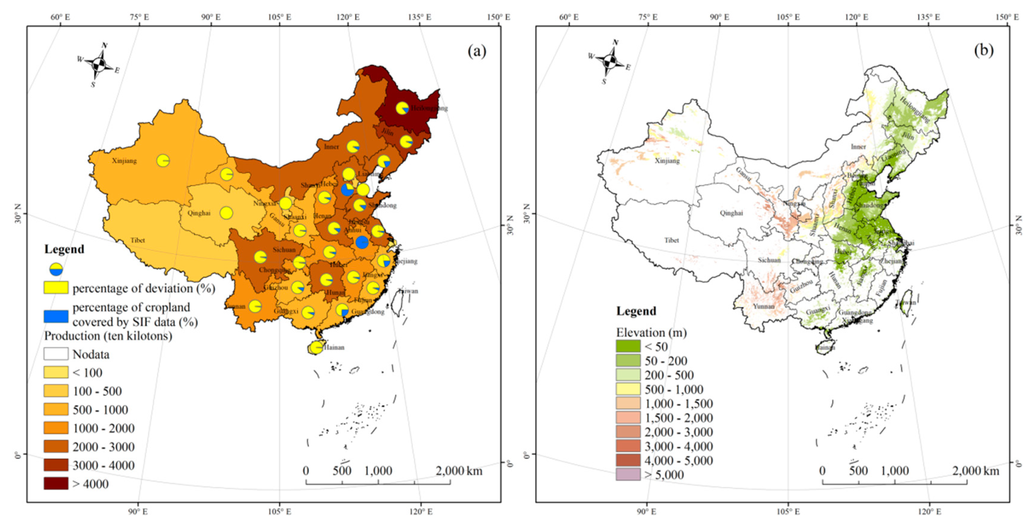
2.1. Study Area

China has an area of 9.6 million km² and it is located in East Asia on the west coast of the Pacific Ocean. Most of continental China is located in the Temperate Zone; the south is located in the tropical and subtropical zones and the north is located near the Polar Zone [34]. In addition, maize, rice, and wheat are the main grains of China [35]. The study area included 34 provincial-level administrative regions, with the exception of Hong Kong, Macau, and Taiwan (Figure 1). No SIF data passed by Shanghai on June and July 2015 and July 2016, and Tibet on June 2015 and July 2016.

2.2. OCO-2 SIF Products

We used the OCO-2 SIF data, which is provided freely from (https://disc.gsfc.nasa.gov) and available from September 2014 to present. The OCO-2 instrument is a three-channel grating spectrometer recorded the high resolution spectra of the O2 A-band (757–775 nm) and the other two bands. Fraunhofer lines at 758.8 and 770.1 nm can be used for the fluorescence retrieval via the FLD (Fraunhofer Line Discrimination) algorithm. Generally, the former is referred as the 757 nm window, with the latter as the 771 nm window [24,26,28,36]. Therefore, OCO-2 provides mid-day SIF retrievals at both 757 and 771 nm. The mid-day SIF products were converted to daily SIF by applying the daily correction factor that was included in the SIF Lite product. The OCO-2 system observed data by three modes, which included nadir, glint, and target. Typical OCO-2 alternately measured between the nadir and glint viewing mode. The repeat frequency of the special target observation mode is approximately 16 days. In the nadir mode, the instrument views the ground directly below the spacecraft. In the glint mode, the instrument tracks near the location with direct sunlight being reflected [29]. Besides, a target mode is infrequently turned on when the satellite overpasses the ground validation sites. In this mode, a large number of temporally continuous measurements at different viewing zenith angles (VZA) are made [37]. Details of the retrieval that is based on the IMAP-DOAS (Iterative Maximum A Posteriori-Differential Optical Absorption Spectroscopy) preprocessor, as well as the OCO-2 SIF product can be found in Frankenberg et al. [26,28], which is also efficient in removing low and thick clouds. In this study, we used the SIF Lite product (V8r) aggregated as daily files with 1.29 × 2.25 km² spatial resolution.

2.3. MODIS Products

MODIS VIs and land cover type products were used in this study. These data were freely provided from (https://e4ftl01.cr.usgs.gov).

The NDVI and EVI are two commonly-used VIs for monitoring vegetation conditions. These VIs have significant relationships with crop production [38]. We used monthly NDVI and EVI derived from MOD13A3 data, with 1 km spatial resolution. The algorithm ingests all the 16-day 1 km products that overlap the month and employ a weighted temporal average.

$$NDVI=\frac{NIR-Red}{NIR+Red}$$

(1)

$$EVI=G\frac{NIR-Red}{NIR+C1Red-C2Blue+L}$$

(2)

where $Red$ (620–670 nm), $NIR$ (841–876 nm), and $Blue$ (459–479 nm) are the surface bidirectional reflectance factors for MODIS bands 1, 2, and 3, respectively; $L$ is the canopy background adjustment for correcting the nonlinear, differential NIR, and red radiant transfer through a canopy; $C1$ and $C2$ are the coefficients of the aerosol resistance term (that uses the blue band to correct for aerosol influences in the red band); and, $G$ is a gain or scaling factor. The coefficients adopted for the MODIS EVI algorithm are, $L$ = 1, $C1$= 6, $C2$= 7.5, and $G$ = 2.5 [39].

The MODIS land cover type product (MCD12Q1) provides annual data that characterize five global land cover classification systems from 2001 to present, with the spatial resolution of 500 m. The land cover product that we used is based on the IGBP global vegetation classification scheme.

2.4. Autumn Crop Production Data of China

The autumn crop production data of each province in China are available at the official website of the National Bureau of Statistics (http://data.stats.gov.cn). The statistical data that we can obtain on this website were updated to 2016. In addition to Hong Kong, Macau, and Taiwan, the autumn crop production data were obtained of each province in 2015 and 2016. The autumn crop production can reach up to 60 million tons in areas with large cropland (e.g., Heilongjiang) and less than one million ton in areas with small cropland (e.g., Beijing, Hainan, and Shanghai).

2.5. Analysis

According to the definition of autumn crop, the final production is most related to the summer season. The satellite-derived data from June to August 2015 and 2016 were extracted while using the following processes. Firstly, we extracted “SIF 757 nm” and “SIF 771 nm” values (henceforth denoted as SIF757 and SIF771), where the land cover type was cropland with an IGBP index of 12 and removed the negative values, which may affect the results. The SIF data were created as a grid map and resampled to 500 m spatial resolution. Subsequently, the VIs data were also resampled to the same spatial resolution and masked with the cropland data to obtain the cropland VIs data. The cropland data of 2015 and 2016 were obtained from the MCD12Q1 product, respectively. These satellite-derived data were used zonal statistics for 31 China provinces at monthly and seasonal scales by means of ArcGIS10.1 (ESRI, Redlands, CA, USA) to obtain the mean pixel value and the cropland pixels for each province.

The converted value was the mean pixel value, multiplied by the cropland pixels. These converted values were henceforth denoted as SIF757’, SIF771’, EVI’, and NDVI’. The relationships of these converted values with autumn crop production statistics were evaluated at monthly and seasonal timescales while using the following equation:

$$Valu{e}_i{}^{\prime } = \overline{Valu{e}_i}\times n_i$$

(3)

where $Valu{e}_i{}^{\prime }$ and $\overline{Valu{e}_i}$ represented the converted satellite-derived product value and the mean satellite-derived product pixel value for each province, respectively; $n_i$ represented the cropland pixels for each province; and, $i$, which ranged from 1 to 31, represented the province where the statistical data were available when the SIF data passed by.

To compare the potential of OCO-2 SIF and MODIS VIs in estimating autumn crop production, the correlations between the converted OCO-2 SIF products (SIF757, SIF771), MODIS VIs (EVI, NDVI), and the government’s autumn crop production statistics were evaluated at monthly and seasonal scales. The SIF data were spatially discrete points, because the viewing modes alternate from orbit to orbit. We calculated the value at a monthly scale while using the points that passed by in June, July, and August, respectively. Subsequently, the values at a seasonal scale using the total points of summer (June, July, and August) were calculated. We obtained the monthly scale value directly and calculated the value at seasonal scale while using the average of June, July, and August data since VIs were monthly raster data.

The correlations between SIF757’, SIF771’, EVI’, NDVI’, and autumn crop production were evaluated while using the coefficient of determination (R²). Root mean square error (RMSE) and mean absolute error (MAE) [6,40] were used to evaluate the performance of crop production estimation. The indicators were calculated while using the following equations:

$$R^2=1-\frac{{{\displaystyle \sum }}_1^n{\left(y_i-\widehat{y_i}\right)}^2}{{{\displaystyle \sum }}_1^n{y}_i^2}$$

(4)

$$RMSE=\sqrt{\frac{{{\displaystyle \sum }}_1^n{\left(y_i-\widehat{y_i}\right)}^2}{n}}$$

(5)

$$MAE=\frac{{{\displaystyle \sum }}_1^n\left|y_i-\widehat{y_i}\right|}{n}$$

(6)

where $n$ was the number of provinces used for validation. $\widehat{y_i}$ was the SIF757’, SIF771’, EVI’, NDVI’ (Equation (4)), and estimated autumn crop production (Equations (5) and (6)). Additionally, $y_i$ was the government’s autumn crop production statistics (ten kilotons).

All of the statistical analyzes were performed while using SPSS Statistics 22 (IBM, Chicago, IL, USA), Origin2017 (OriginLab, Northampton, MA, USA), and MATLAB R2017b (MathWorks, Nadick, MA, USA). Generally, the optimal result is judged by a maximum R² value, minimum RMSE, and MAE values.

In addition, the relationships between SIF757’, SIF771’, EVI’, NDVI’, and the autumn crop production statistics were modeled based on the most relevant month or season data in 2015. The models whose R² is highest in June, July, August, and summer were selected as the most relevant models and they were used to estimate the 2016 autumn crop production. The model with the best performance was specifically analyzed.

3. Results

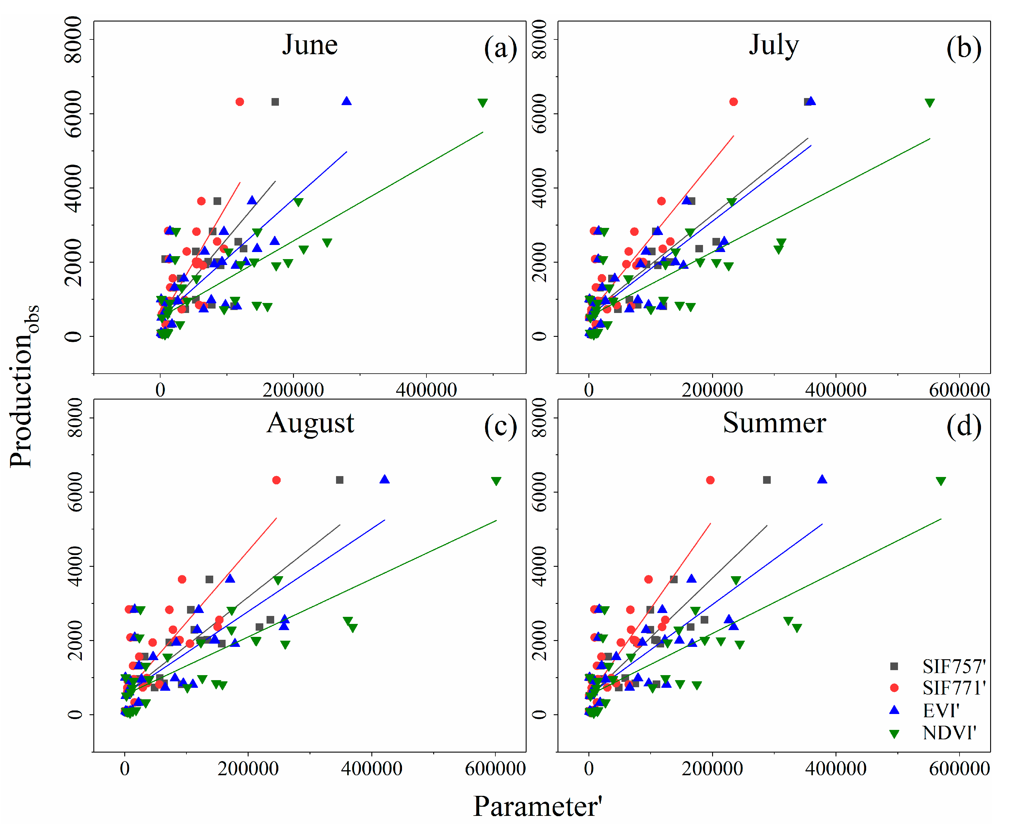
3.1. Relationships of OCO-2 SIF and MODIS VIs with Autumn Crop Production at Monthly and Seasonal Scales

We compared the relationship between the SIF757’, SIF771’, EVI’, NDVI’, and the government’s autumn crop production statistics at monthly and seasonal scales. The results for the 2015 summer show that the converted OCO-2 SIF data, MODIS VIs, and the government’s autumn crop production statistics were strongly correlated (Figure 2). In general, SIF771’ (R² = 0.548–0.716, p < 0.01) was more strongly correlated with the government’s autumn crop production statistics than SIF757’ (R² = 0.526–0.692, p < 0.01). In addition, EVI’ (R² = 0.628–0.664, p < 0.01) and NDVI’ (R² = 0.666–0.672, p < 0.01) had equally strong correlations with the government’s autumn crop production statistics.

The strongest relationship of SIF757’ (R² = 0.692, p < 0.01), SIF771’ (R² = 0.716, p < 0.01), EVI’ (R² = 0.664, p < 0.01), and NDVI’ (R² = 0.672, p < 0.01) was observed in July (Figure 2b). The mean R² of SIF757’ and SIF771’ were 0.643 and 0.662. Additionally, the mean R² of EVI’ and NDVI’ were 0.650 and 0.668. Moreover, the correlation between SIF’ and autumn crop production was higher than VIs’ for both monthly and seasonal scales, except in June, during the summer of 2015 (

Table 1. The correlations between the SIF757’, SIF771’, EVI’, NDVI’, and the government’s autumn crop production statistics in China during June to August 2015 at monthly and seasonal scales.

	June				July
	SIF757’	SIF771’	EVI’	NDVI’	SIF757’	SIF771’	EVI’	NDVI’
R2	0.526	0.548	0.628	0.667	0.692	0.716	0.664	0.672
p-value	<0.01				<0.01
	August				Summer
	SIF757’	SIF771’	EVI’	NDVI’	SIF757’	SIF771’	EVI’	NDVI’
R2	0.669	0.683	0.652	0.666	0.686	0.702	0.656	0.666
p-value	<0.01				<0.01

). In addition, the correlation between VIs’ (EVI’ and NDVI’) and autumn crop production do not greatly vary among months. By contrast, the correlation between SIF’ (SIF757’ and SIF771’) and autumn crop production among the months exhibited great variation.

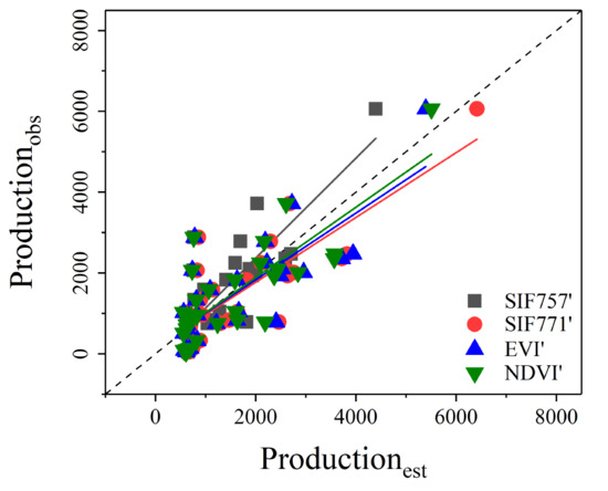
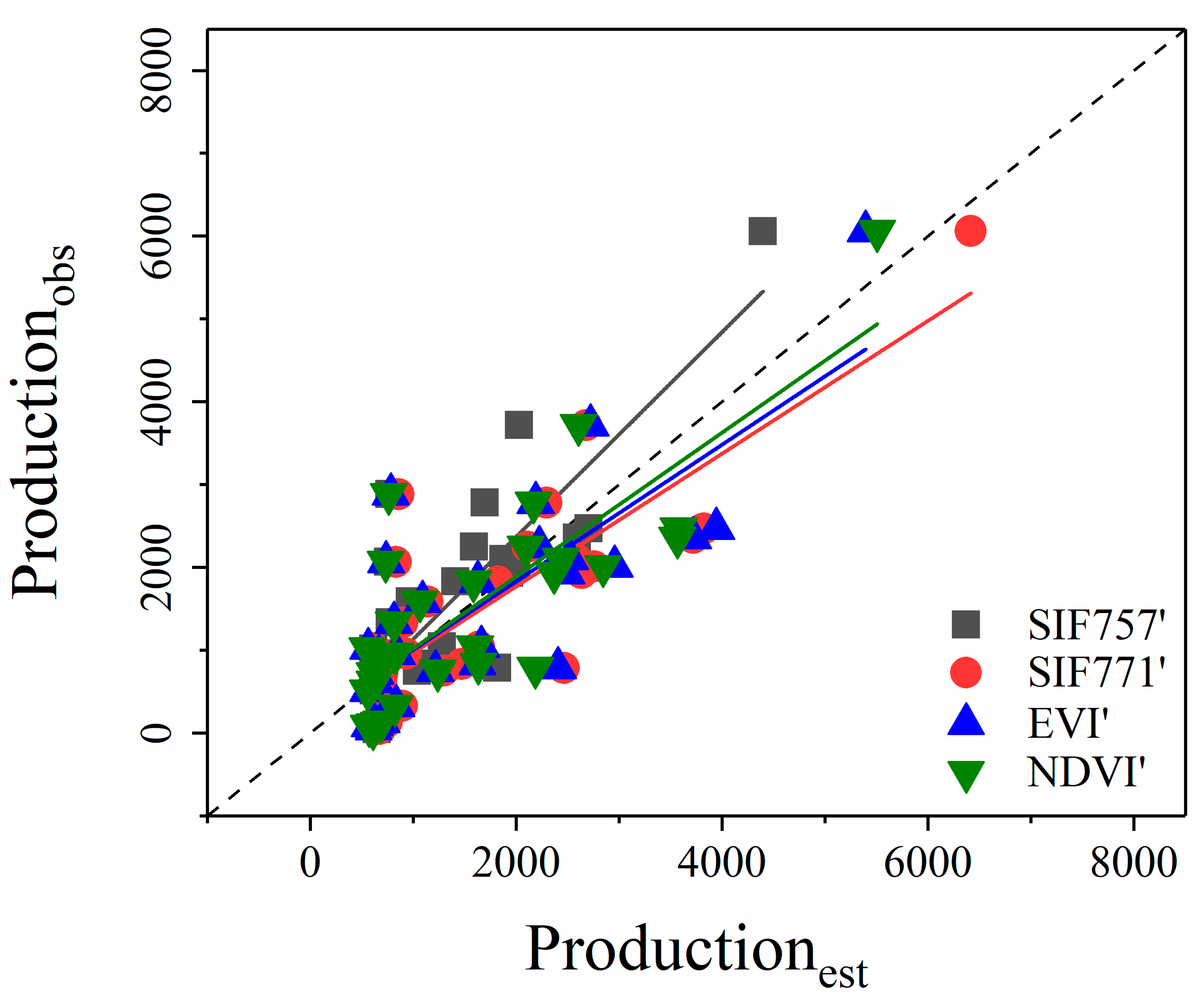
3.2. Performance Evaluation of the Autumn Crop Production Estimated by the Converted OCO-2 SIF and MODIS VIs

The SIF’ and VIs’ in July had the strongest correlation with the autumn crop production statistics according to the relationship between the SIF757’, SIF771’, EVI’, NDVI’, and the government’s autumn crop production statistics in the summer of 2015 (Figure 2 and Table 1). 4 models con be chosen to estimate autumn crop production (

Table 2. Best-fit models for each parameter’, which was used to estimate the autumn crop production in China.

Time	Parameter’	Model	N	R2	p-Value
July	SIF757’	$\widehat{y_i}=0.01338\times x_i+604.01428$	30	0.692	<0.01
	SIF771’	$\widehat{y_i }=0.02050\times x_i+608.13718$	30	0.716	<0.01
	EVI’	$\widehat{y_i}=0.01280\times x_i+547.13583$	30	0.664	<0.01
	NDVI’	$\widehat{y_i}=0.00869\times x_i+540.97517$	30	0.672	<0.01

Note: $\widehat{y_i}$ represents the estimated autumn crop production; $x_i$ represents SIF757’, SIF771’, EVI’ and NDVI’, respectively.

). The fitted models with p-values that were lower than 0.01 indicated a significant relationship between the SIF757’, SIF771’, EVI’, NDVI’, and the government’s autumn crop production statistics, and confirmed the reliable predictive capability of these models.

Growing evidence suggested that the relationship between vegetation photosynthesis (gross primary productivity, GPP) and SIF is linearly related [41,42,43,44,45]. Moreover, terrestrial GPP drives the terrestrial food chain [46]. Therefore, we assumed that SIF and production are related linearly and selected the linear model to predict the autumn crop production. The linear models in July (Table 2) were utilized to estimate autumn crop production in each province in 2016 (Figure 3). 2016 was the only one year in which OCO-2 SIF product, MODIS VIs products, and the government’s autumn crop production statistics data could be matched, except for 2015. The robustness of the coefficients derived from these production estimation models for each province in 2016 was evaluated while using RMSE and MAE. The scatterplots between the production statistics and estimated productions demonstrated satisfactory results (Figure 3). The estimated autumn crop productions of each model were close to the government’s autumn crop production statistics in 2016 (

Table 3. The comparisons between the estimated autumn crop productions using the SIF757’, SIF771’, EVI’, NDVI’, and the government’s autumn crop production statistics in China in 2016.

	July
Parameter	SIF757’	SIF771’	EVI’	NDVI’
R2	0.678	0.673	0.620	0.647
p	<0.01	<0.01	<0.01	<0.01
RMSE (ten kilotons)	748.901	754.852	813.066	783.330
MAE (ten kilotons)	567.629	619.806	649.126	620.205

). Moreover, the performances of SIF757’, SIF771’, EVI’, and NDVI’ are comparable. The best performance was observed in the autumn crop productions that were estimated using SIF757’ in July (R² = 0.678, p < 0.01; RMSE = 748.901 ten kilotons; MAE = 567.629 ten kilotons).

The OCO-2 SIF products performed better than MODIS VIs products when estimating the autumn crop production and SIF757’ performed best. We conducted a detailed analysis of the estimation of SIF757’ in order to identify the constraints that affect the estimation accuracy of SIF (Figure 4). We calculated the deviation percentage of the autumn crop production estimated while using SIF757 in 2016, and the percentage of cropland that was covered by SIF data in each province. Meanwhile, the minimum percentage of cropland covered by SIF data is up to 3.762% (Anhui) and the maximum percentage of cropland covered by SIF data is up to 4.524% (Heilongjiang).

The lower the percentage of cropland covered by SIF data, the higher the deviation percentage of autumn crop production estimated while using the SIF757’. Meanwhile, in Beijing, Hainan, Qinghai, Tianjin, Ningxia, and Xinjiang, where the autumn crop production is approximately less than five million tons and the elevation is higher than 1000 m, the deviation percentage of autumn crop production estimated using the SIF757’ exceeded 100% (Figure 4a). Besides, in Sichuan, Chongqing, Hunan, Shaanxi, and other provinces with large undulating terrain and broken cropland, the autumn crop production that was estimated using the SIF757’ was also not very accurate (Figure 4).

4. Discussion

4.1. Potential of OCO-2 SIF and MODIS VIs in Estimating the Autumn Crop Production of China

The main goals of this study are (1) to explore the relationship between the OCO-2 SIF data and the government’s autumn crop production statistics and establish a simplified model for estimating autumn crop production while using OCO-2 SIF; (2) to compare the differences between the SIF757’, SIF771’, EVI’, NDVI’ for estimating the autumn crop production; and, (3) to analyze the factors affecting the estimation accuracy. Therefore, it is a new attempt to use satellite remote SIF data for crop production estimation.

Crops yield can be estimated while using remotely sensed GPP [47]. Additionally, GPP based on GOME-2 SIF has been used to predict the crop yield in previous study [46]. Thus, GPP and crop yield (production) are related. On the other hand, SIF is mainly determined by Absorbed photosynthetically active radiation (APAR) [30,48], which is the key to link SIF and GPP [45]. Therefore, we conclude that OCO-2 SIF data are closely related to autumn crop production. Besides, the spatial resolution of MODIS VIs is finer than OCO-2 SIF and the OCO-2 SIF product is discrete, which indicates that VIs is more advantageous than SIF. However, the autumn crop production that is predicted by SIF’ is more accurate than VIs’, with higher R², lower RMSE, and MAE. It proved that SIF’ is more effective than VIs’.

In addition, the R² of SIF’-crop production statistics were 0.548-0.716 for SIF771’ and they were 0.526–0.692 for SIF757’ (Table 1). The mean R² of SIF’-crop production statistics were 0.662 and 0.643 for SIF771’ and SIF757’, respectively (Table 1). SIF771’ was more related to the autumn crop production than SIF757’. However, SIF757’ performed better than SIF771’ when estimating autumn crop production, which indicated that SIF757 is more sensitive to photosynthesis than SIF771 in this study region. The result is consistent with another study, which showed that SIF757 has a stronger correlation with tower GPP than SIF771 [24]. This phenomenon could be explained by 771 nm falling farther away from the peak emission on the SIF spectrum, which indicated that SIF757 has higher retrieval precision than SIF771 [28,30].

The crop production statistics were highly correlated with EVI/NDVI data during the leaf constant period. In this study, the autumn crop production statistics were more strongly correlated with SIF data during July than the other period, which is the leaf constant period. This finding can be explained by the strong photosynthesis during the constant leaf period. In addition, according to previous studies, July represents the peak growing season for autumn crop [31], which explains why the most relevant correlation between SIF and production is July. SIF757’ performed best when estimating the autumn crop production in China (R² = 0.678, p < 0.01; RMSE = 748.901 ten kilotons; MAE = 567.629 ten kilotons). The performance of SIF757’ is better than the estimation performance of satellite Earth Observation (EO) time-series products for wheat, barley, and grain maize productions in Europe (approximately R² = 0.583) [49]. Moreover, this performance is close to the crop phenology and a combination of EVI2 (the MODIS two-band Enhanced Vegetation Index) and NDVI estimating maize, soybean productions in America (approximately R² = 0.69–0.70) [16].

In addition, the correlations between VIs’ (EVI’ and NDVI’) and autumn crop production were not much different among the months, whereas the correlations between SIF’ (SIF757’ and SIF771’) and autumn crop production were much different among months. This result reveals that SIF can monitor crop dynamics better than VIs, which is in good agreement with the previous results [50,51,52,53], suggesting that SIF is able to precisely track the seasonality of photosynthesis and NDVI is insensitive to seasonal changes in photosynthesis. This finding further indicates that it is feasible to estimate autumn crop production while using satellite-derived SIF products. Additionally, the performance is better and more reliable than VIs.

4.2. Limitation and Uncertainty

In this study, we determined that predicting autumn crop production while using OCO-2 SIF product is feasible and not inferior to MODIS VIs, especially, the performance of SIF757 is best. However, some uncertainties and limitations remain. First of all, the SIF values of each province were obtained by point averaging due to the discrete of OCO-2 SIF product. Moreover, in some provinces, few data passed by their cropland and the mean pixel value of SIF product may not represent the SIF value of the entire cropland. This condition may lead to the inaccuracy of the SIF values. Figure 4 shows the higher the percentage of cropland covered by SIF data, the higher accuracy. This further illustrates that the discrete influences the estimation accuracy. Although the OCO-2 SIF product that we use has the highest spatial resolution available today, it is still relatively coarse. The coarse spatial resolution indicates that the SIF value of each pixel is a mixture of cropland and other vegetation types. The SIF value we used is inaccuracy, which leads to an inaccurate estimation. We found that the accuracy of autumn crop prediction is higher in low-elevation provinces with large farm size and flat cropland by comparing the spatial distribution of Chinese cropland topography with the deviation percentage of autumn crop production estimated using SIF757 (Figure 4) (e.g., Anhui, Hebei, Henan, and so on). This is also affected by the coarse spatial resolution. Moreover, the production of most provinces is between 500 and 4000 ten kilotons, which leads to higher estimation accuracy in these provinces. In addition, the spatial distribution of autumn crops is quite important for accurately estimating the crop yield. However, the data is lacked until now, and it remains hard to distinguish the different crop types using satellite remote sensing for a large area. Therefore, this study mixed all the autumn crops together. Actually, the relationships between SIF and crop production may vary among the different autumn crops due to the influence of the canopy structure, photosynthetic pathways, light energy utilization rate, and C-N carbohydrate conversion capacity, which may constrain the accuracy in estimating autumn crop yields. Besides, the study period (two years) is short due to the limitation of SIF product and statistical data, which may lead to inaccurate results. we still believed that the results were significant since the fitted model with p-values lower than 0.01.

The results can be generalized to other regions and crops, due to the similarity of the SIF generation process. SIF is generated during the photosynthesis process, regardless of the region or crop, which provides a possibility for SIF to estimate crop production. More and more researchers pay attention to satellite-derived SIF, which promotes the development of satellite-derived SIF. New or future missions (e.g., GOSIIF; Tropospheric Monitoring Instrument, TROPOMI; Fluorescence EXplorer, FLEX) with finer spatial resolution and continuous data could be used in a similar study of crop estimation. If possible, our future studies will be conducted in a larger region and more crops with considering more factors.

5. Conclusions

This study explored the potential of OCO-2 SIF product in estimating autumn crop production in China. SIF is generated during the photosynthesis process, which leads to a closer connection between SIF and crop production. The results showed that OCO-2 SIF757 of July had great potential in estimating autumn crop production. The estimation accuracy was limited by the spatial resolution and discrete of satellite-derived SIF product. SIF performs better than VIs in estimating autumn crop production and SIF could monitor crop dynamics more effectively than VIs. With the development of continuous SIF product, such as GOSIF (0.05 degree) [30], TROPOMI (7 km) [54], and FLEX (300 m) [55], we believed that SIF would provide an increasingly accurate crop production estimation. SIF will be widely used in more studies that are related to terrestrial ecosystem and carbon cycles.

References

1. Yu, Q.; Hu, Q.; Vliet, J.V.; Verburg, P.H.; Wu, W. GlobeLand30 shows little cropland area loss but greater fragmentation in China. Int. J. Appl. Earth Obs. 2018, 66, 37–45. [Google Scholar] [CrossRef]
2. Fan, S.; Zhang, X. Production and Productivity Growth in Chinese Agriculture: New National and Regional Measures. Econ. Dev. Cult. Chang. 2002, 50, 819–838. [Google Scholar] [CrossRef]
3. Zhang, F.; Cui, Z.; Fan, M.; Zhang, W.; Chen, X.; Jiang, R. Integrated Soil-Crop System Management: Reducing Environmental Risk while Increasing Crop Productivity and Improving Nutrient Use Efficiency in China. J. Environ. Qual. 2011, 40, 1051–1057. [Google Scholar] [CrossRef] [PubMed]
4. Liu, D.X.; Zhao, H.Y.; Dong, A.X.; Yang, S.H. Impact of Climate Warming on Summer-Autumn Crop Planting Structure in Gansu Province. J. Glaciol. Geocryol. 2005, 27, 806–812. [Google Scholar]
5. Johnson, M.D.; Hsieh, W.W.; Cannon, A.J.; Davidson, A.; Bédard, F. Crop yield forecasting on the Canadian Prairies by remotely sensed vegetation indices and machine learning methods. Agric. For. Meteorol. 2016, 218–219, 74–84. [Google Scholar] [CrossRef]
6. Son, N.T.; Chen, C.F.; Chen, C.R.; Minh, V.Q.; Trung, N.H. A comparative analysis of multitemporal MODIS EVI and NDVI data for large-scale rice yield estimation. Agric. For. Meteorol. 2014, 197, 52–64. [Google Scholar] [CrossRef]
7. Moran, M.S.; Inoue, Y.; Barnes, E.M. Opportunities and limitations for image-based remote sensing in precision crop management. Remote Sens. Environ. 1997, 61, 319–346. [Google Scholar] [CrossRef]
8. Shanahan, J.F.; Schepers, J.S.; Francis, D.D.; Varvel, G.E.; Wilhelm, W.W.; Tringe, J.M.; Schlemmer, M.R.; Major, D.J. Use of Remote-Sensing Imagery to Estimate Corn Grain Yield. Agron. J. 2001, 93, 583–589. [Google Scholar] [CrossRef]
9. Pjjr, P.; Hatfield, J.L.; Schepers, J.S.; Barnes, E.M.; Moran, M.S.; Cst, D.; Upchurch, D.R. Remote sensing for crop management. Photogramm. Eng. Remote Sens. 2003, 69, 647–664. [Google Scholar]
10. Baret, F.; Houlès, V.; Guérif, M. Quantification of plant stress using remote sensing observations and crop models: The case of nitrogen management. J. Exp. Bot. 2007, 58, 869–880. [Google Scholar] [CrossRef]
11. Calera, A.; Campos, I.; Osann, A.; D’Urso, G.; Menenti, M. Remote Sensing for Crop Water Management: From ET Modelling to Services for the End Users. Sensors 2017, 17, 1104. [Google Scholar] [CrossRef] [PubMed]
12. Chaudhari, K.N.; Tripathy, R.; Patel, N.K. Spatial wheat yield prediction using crop simulation model, GIS, remote sensing and ground observed data. J. Agrometeorol. 2010, 12, 174–180. [Google Scholar]
13. Ju, W.M.; Ping, G.; Zhou, Y.L.; Chen, J.M.; Shu, C.; Li, X.F.; Gong, P.; Howarth, P.J.; Xu, B.; Ju, W. Prediction of summer grain crop yield with a process-based ecosystem model and remote sensing data for the northern area of the Jiangsu Province, China. Int. J. Remote Sens. 2010, 46, 1573–1587. [Google Scholar] [CrossRef]
14. Li, A.; Liang, S.; Wang, A.; Qin, J. Estimating Crop Yield from Multi-temporal Satellite Data Using Multivariate Regression and Neural Network Techniques. Photogramm. Eng. Remote Sens. 2013, 73, 1149–1157. [Google Scholar] [CrossRef]
15. Singleton, A.; Li, Z.; Hoey, T.; Muller, J.P. Evaluating sub-pixel offset techniques as an alternative to D-InSAR for monitoring episodic landslide movements in vegetated terrain. Remote Sens. Environ. 2014, 147, 133–144. [Google Scholar] [CrossRef] [Green Version]
16. Bolton, D.K.; Friedl, M.A. Forecasting crop yield using remotely sensed vegetation indices and crop phenology metrics. Agric. For. Meteorol. 2013, 173, 74–84. [Google Scholar] [CrossRef]
17. Mkhabela, M.S.; Bullock, P.; Raj, S.; Wang, S.; Yang, Y. Crop yield forecasting on the Canadian Prairies using MODIS NDVI data. Agric. For. Meteorol. 2011, 151, 385–393. [Google Scholar] [CrossRef]
18. Johnson, D.M. An assessment of pre- and within-season remotely sensed variables for forecasting corn and soybean yields in the United States. Remote Sens. Environ. 2014, 141, 116–128. [Google Scholar] [CrossRef]
19. Shao, Y.; Campbell, J.B.; Taff, G.N.; Zheng, B. An analysis of cropland mask choice and ancillary data for annual corn yield forecasting using MODIS data. Int. J. Appl. Earth Obs. 2015, 38, 78–87. [Google Scholar] [CrossRef]
20. Meroni, M.; Rossini, M.; Guanter, L.; Alonso, L.; Rascher, U.; Colombo, R.; Moreno, J. Remote sensing of solar-induced chlorophyll fluorescence: Review of methods and applications. Remote Sens. Environ. 2009, 113, 2037–2051. [Google Scholar] [CrossRef]
21. Zhang, Y.; Xiao, X.; Jin, C.; Dong, J.; Zhou, S.; Wagle, P.; Joiner, J.; Guanter, L.; Zhang, Y.; Zhang, G.; et al. Consistency between sun-induced chlorophyll fluorescence and gross primary production of vegetation in North America. Remote Sens. Environ. 2016, 183, 154–169. [Google Scholar] [CrossRef] [Green Version]
22. Grace, J.; Nichol, C.; Disney, M.; Lewis, P.; Quaife, T.; Bowyer, P. Can we measure terrestrial photosynthesis from space directly, using spectral reflectance and fluorescence? Glob. Chang. Biol. 2007, 13, 1484–1497. [Google Scholar] [CrossRef]
23. Baker, N.R. Chlorophyll fluorescence: A probe of photosynthesis in vivo. Annu. Rev. Plant. Biol. 2008, 59, 89–113. [Google Scholar] [CrossRef]
24. Li, X.; Xiao, J.; He, B. Chlorophyll fluorescence observed by OCO-2 is strongly related to gross primary productivity estimated from flux towers in temperate forests. Remote Sens. Environ. 2018, 204, 659–671. [Google Scholar] [CrossRef]
25. Zarco-Tejada, P.J.; Morales, A.; Testi, L.; Villalobos, F.J. Spatio-temporal patterns of chlorophyll fluorescence and physiological and structural indices acquired from hyperspectral imagery as compared with carbon fluxes measured with eddy covariance. Remote Sens. Environ. 2013, 133, 102–115. [Google Scholar] [CrossRef]
26. Frankenberg, C.; Fisher, J.B.; Worden, J.; Badgley, G.; Saatchi, S.S.; Lee, J.-E.; Toon, G.C.; Butz, A.; Jung, M.; Kuze, A.; et al. New global observations of the terrestrial carbon cycle from GOSAT: Patterns of plant fluorescence with gross primary productivity. Geophys. Res. Lett. 2011, 38, L17706. [Google Scholar] [CrossRef]
27. Joiner, J.; Yoshida, Y.; Vasilkov, A.P.; Yoshida, Y.; Corp, L.A.; Middleton, E.M. First observations of global and seasonal terrestrial chlorophyll fluorescence from space. Biogeosciences 2011, 8, 637–651. [Google Scholar] [CrossRef] [Green Version]
28. Frankenberg, C.; O’Dell, C.; Berry, J.; Guanter, L.; Joiner, J.; Köhler, P.; Pollock, R.; Taylor, T.E. Prospects for chlorophyll fluorescence remote sensing from the Orbiting Carbon Observatory-2. Remote Sens. Environ. 2014, 147, 1–12. [Google Scholar] [CrossRef] [Green Version]
29. Li, X.; Xiao, J.; He, B.; Altaf Arain, M.; Beringer, J.; Desai, A.R.; Emmel, C.; Hollinger, D.Y.; Krasnova, A.; Mammarella, I.; et al. Solar-induced chlorophyll fluorescence is strongly correlated with terrestrial photosynthesis for a wide variety of biomes: First global analysis based on OCO-2 and flux tower observations. Glob. Chang. Biol. 2018, 24, 3990–4008. [Google Scholar] [CrossRef]
30. Li, X.; Xiao, J. A Global, 0.05-Degree Product of Solar-Induced Chlorophyll Fluorescence Derived from OCO-2, MODIS, and Reanalysis Data. Remote Sens. 2019, 11, 517. [Google Scholar] [CrossRef]
31. Zhang, Y.G.; Guanter, L.; Berry, J.A.; Joiner, J.; van der Tol, C.; Huete, A.; Gitelson, A.; Voigt, M.; Kohler, P. Estimation of vegetation photosynthetic capacity from space-based measurements of chlorophyll fluorescence for terrestrial biosphere models. Glob. Chang. Biol. 2014, 20, 3727–3742. [Google Scholar] [CrossRef] [Green Version]
32. Guanter, L.; Zhang, Y.G.; Jung, M.; Joiner, J.; Voigt, M.; Berry, J.A.; Frankenberg, C.; Huete, A.R.; Zarco-Tejada, P.; Lee, J.E.; et al. Global and time-resolved monitoring of crop photosynthesis with chlorophyll fluorescence. Proc. Natl. Acad. Sci. USA 2014, 111, 1327–1333. [Google Scholar] [CrossRef]
33. Guan, K.; Wu, J.; Kimball, J.S.; Anderson, M.C.; Frolking, S.; Li, B.; Hain, C.R.; Lobell, D.B. The shared and unique values of optical, fluorescence, thermal and microwave satellite data for estimating large-scale crop yields. Remote Sens. Environ. 2017, 199, 333–349. [Google Scholar] [CrossRef] [Green Version]
34. Zou, C.; Gao, X.; Shi, R.; Fan, X.; Zhang, F. Micronutrient Deficiencies in Crop Production in China. In Micronutrient Deficiencies in Global Crop Production, 1st ed.; Alloway, B.J., Ed.; Springer: Dordrecht, The Netherlands, 2008; pp. 127–148. [Google Scholar]
35. Fusuo, Z.; Xinping, C.; Peter, V. Chinese agriculture: An experiment for the world. Nature 2013, 497, 33–35. [Google Scholar]
36. Du, S.; Liu, L.; Liu, X.; Zhang, X.; Zhang, X.; Bi, Y.; Zhang, L. Retrieval of global terrestrial solar-induced chlorophyll fluorescence from TanSat satellite. Sci. Bull. 2018, 63, 1502–1512. [Google Scholar] [CrossRef] [Green Version]
37. Sun, Y.; Frankenberg, C.; Jung, M.; Joiner, J.; Guanter, L.; Köhler, P.; Magney, T. Overview of Solar-Induced chlorophyll Fluorescence (SIF) from the Orbiting Carbon Observatory-2: Retrieval, cross-mission comparison, and global monitoring for GPP. Remote Sens. Environ. 2018, 209, 808–823. [Google Scholar] [CrossRef]
38. Dong, J.; Xiao, X.; Wagle, P.; Zhang, G.; Zhou, Y.; Jin, C.; Torn, M.S.; Meyers, T.P.; Suyker, A.E.; Wang, J.; et al. Comparison of four EVI-based models for estimating gross primary production of maize and soybean croplands and tallgrass prairie under severe drought. Remote Sens. Environ. 2015, 162, 154–168. [Google Scholar] [CrossRef] [Green Version]
39. Huete, A.; Didan, K.; Miura, T.; Rodriguez, E.P.; Gao, X.; Ferreira, L.G. Overview of the radiometric and biophysical performance of the MODIS vegetation indices. Remote Sens. Environ. 2002, 83, 195–213. [Google Scholar] [CrossRef]
40. Wei, J.; Chen, Y.; Gu, Q.; Jiang, C.; Ma, M.; Song, L.; Tang, X. Potential of the remotely-derived products in monitoring ecosystem water use efficiency across grasslands in Northern China. Int. J. Remote Sens. 2019, 40, 6203–6223. [Google Scholar] [CrossRef]
41. Sun, Y.; Frankenberg, C.; Wood, J.D.; Schimel, D.S.; Jung, M.; Guanter, L.; Drewry, D.T.; Verma, M.; Porcar-Castell, A.; Griffis, T.J.; et al. OCO-2 advances photosynthesis observation from space via solar-induced chlorophyll fluorescence. Science 2017, 358, eaam5747. [Google Scholar] [CrossRef] [Green Version]
42. Verma, M.; Schimel, D.; Evans, B.; Frankenberg, C.; Beringer, J.; Drewry, D.T.; Magney, T.; Marang, I.; Hutley, L.; Moore, C. Effect of environmental conditions on the relationship between solar-induced fluorescence and gross primary productivity at an OzFlux grassland site. J. Geophys. Res. 2017, 122, 716–733. [Google Scholar] [CrossRef]
43. Guanter, L.; Frankenberg, C.; Dudhia, A.; Lewis, P.E.; Gómez-Dans, J.; Kuze, A.; Suto, H.; Grainger, R.G. Retrieval and global assessment of terrestrial chlorophyll fluorescence from GOSAT space measurements. Remote Sens. Environ. 2012, 121, 236–251. [Google Scholar] [CrossRef]
44. Liu, L.; Guan, L.; Liu, X. Directly estimating diurnal changes in GPP for C3 and C4 crops using far-red sun-induced chlorophyll fluorescence. Agric. For. Meteorol. 2017, 232, 1–9. [Google Scholar] [CrossRef]
45. Du, S.; Liu, L.; Liu, X.; Hu, J. Response of Canopy Solar-Induced Chlorophyll Fluorescence to the Absorbed Photosynthetically Active Radiation Absorbed by Chlorophyll. Remote Sens. 2017, 9, 911. [Google Scholar] [CrossRef]
46. Heimann, M.; Reichstein, M. Terrestrial ecosystem carbon dynamics and climate feedbacks. Nature 2008, 451, 289–292. [Google Scholar] [CrossRef]
47. Jaafar, H.H.; Ahmad, F.A. Crop yield prediction from remotely sensed vegetation indices and primary productivity in arid and semi-arid lands. Int. J. Remote Sens. 2015, 36, 4570–4589. [Google Scholar] [CrossRef]
48. Miao, G.; Guan, K.; Yang, X.; Bernacchi, C.J.; Berry, J.A.; DeLucia, E.H.; Wu, J.; Moore, C.E.; Meacham, K.; Cai, Y.; et al. Sun-Induced Chlorophyll Fluorescence, Photosynthesis, and Light Use Efficiency of a Soybean Field from Seasonally Continuous Measurements. J. Geophys. Res. Biogosci. 2018, 123, 610–623. [Google Scholar] [CrossRef]
49. López-Lozano, R.; Duveiller, G.; Seguini, L.; Meroni, M.; García-Condado, S.; Hooker, J.; Leo, O.; Baruth, B. Towards regional grain yield forecasting with 1km-resolution EO biophysical products: Strengths and limitations at pan-European level. Agric. For. Meteorol. 2015, 206, 12–32. [Google Scholar] [CrossRef]
50. Damm, A.; Elbers, J.; Erler, A.; Gioli, B.; Hamdi, K.; Hutjes, R.; Kosvancova, M.; Meroni, M.; Miglietta, F.; Moersch, A.; et al. Remote sensing of sun-induced fluorescence to improve modeling of diurnal courses of gross primary production (GPP). Glob. Chang. Biol. 2010, 16, 171–186. [Google Scholar] [CrossRef]
51. Flexas, J.; Escalona, J.M.; Evain, S.; Gulias, J.; Moya, I.; Osmond, C.B.; Medrano, H. Steady-state chlorophyll fluorescence (Fs) measurements as a tool to follow variations of net CO2 assimilation and stomatal conductance during water-stress in C-3 plants. Physiol. Plant 2002, 114, 231–240. [Google Scholar] [CrossRef]
52. Meroni, M.; Rossini, M.; Picchi, V.; Panigada, C.; Cogliati, S.; Nali, C.; Colombo, R. Assessing steady-state fluorescence and PRI from hyperspectral proximal sensing as early indicators of plant stress: The case of ozone exposure. Sensors 2008, 8, 1740–1754. [Google Scholar] [CrossRef]
53. Magney, T.S.; Bowling, D.R.; Logan, B.A.; Grossmann, K.; Stutz, J.; Blanken, P.D.; Burns, S.P.; Cheng, R.; Garcia, M.A.; Kӧhler, P.; et al. Mechanistic evidence for tracking the seasonality of photosynthesis with solar-induced fluorescence. Proc. Natl. Acad. Sci. USA 2019, 116, 11640–11645. [Google Scholar] [CrossRef] [Green Version]
54. Guanter, L.; Aben, I.; Tol, P.; Krijger, J.M.; Hollstein, A.; Köhler, P.; Damm, A.; Joiner, J.; Frankenberg, C.; Landgraf, J. Potential of the TROPOspheric Monitoring Instrument (TROPOMI) onboard the Sentinel-5 Precursor for the monitoring of terrestrial chlorophyll fluorescence. Atmos. Meas. Tech. 2014, 7, 12545–12588. [Google Scholar] [CrossRef]
55. Liu, L.; Liu, X.; Hu, J. Effects of spectral resolution and SNR on the vegetation solar-induced fluorescence retrieval using FLD-based methods at canopy level. Eur. J. Remote Sens. 2017, 48, 743–762. [Google Scholar] [CrossRef]
Figure 1. The trajectory of Orbiting Carbon Observatory-2 (OCO-2) passed by cropland from June to August 2015 in China. The land cover map is from the moderate resolution imaging spectroradiometer (MODIS) land cover type product (MCD12Q1) based on the IGBP (International Geosphere-Biosphere Programme) classification scheme.
Remotesensing 11 01715 g001
Figure 2. The correlations between the SIF757’, SIF771’, EVI’, NDVI’, and the government’s autumn crop production statistics (ten kilotons) in China during June to August 2015 at the monthly and seasonal scales. The parameter’ represent SIF757’ (W m−2 sr−1 μm−1), SIF771’ (W m−2 sr−1 μm−1), EVI’, and NDVI’, respectively.
Remotesensing 11 01715 g002
Figure 3. The comparisons between autumn crop production estimated by the SIF757’, SIF771’, EVI’, NDVI’, and the government’s autumn crop production statistics in China in 2016 using July data. Productionobs (ten kilotons) and productionest (ten kilotons) represent production observation and production estimation, respectively.
Remotesensing 11 01715 g003
Figure 4. The spatial distribution of the government’s autumn crop production statistics, the percentage of deviation of the autumn crop production estimated by using SIF757 in 2016, and the percentage of cropland covered by solar-induced chlorophyll fluorescence (SIF) data in each province (a); and, topography of Chinese cropland (b).
Remotesensing 11 01715 g004