Evaluation of an Extended PICS (EPICS) for Calibration and Stability Monitoring of Optical Satellite Sensors

Abstract

Pseudo Invariant Calibration Sites (PICS) have been increasingly used as an independent data source for on-orbit radiometric calibration and stability monitoring of optical satellite sensors. Generally, this would be a small region of land that is extremely stable in time and space, predominantly found in North Africa. Use of these small regions, referred to as traditional PICS, can be limited by: (i) the spatial extent of an individual Region of Interest (ROI) and/or site; (ii) and the frequency of how often the site can be acquired, based on orbital patterns and cloud cover at the site, both impacting the time required to construct a richly populated temporal dataset. This paper uses a new class of continental scaled PICS clusters (also known as Extended PICS or EPICS), to demonstrate their capability in increasing temporal frequency of the calibration time series which ultimately allows calibration and stability assessment at a much finer scale compared to the traditional PICS-based method while also reducing any single location’s potential impact to the overall assessment. The use of EPICS as a calibration site was evaluated using data from Landsat-8 Operational Land Imager (OLI), Landsat 7 Enhanced Thematic Mapper Plus (ETM+), and Sentinel-2A&B Multispectral Instrument (MSI) images at their full spatial resolutions. Initial analysis suggests that EPICS, at its full potential and with nominal cloud consideration, can significantly decrease the temporal revisit interval of moderate resolution sensors to as much as of 0.33 day (3 collects/day). A traditional PICS is expected to have a temporal uncertainty (defined as the ratio of temporal standard deviation and temporal mean) of 2–5% for TOA reflectance. Over the same time period EPICS produced a temporal uncertainty of 3%. But the advantage to be leveraged is the ability to detect sensor change quicker due to the denser dataset and reduce the impact of any potential ‘local’ changes. Moreover, this approach can be extended to any on-orbit sensor. An initial attempt to quantify the minimum detectable change (a threshold slope value which must be exceeded by the reflectance trend to be considered statistically significant) suggests that the use of EPICS can decrease the time period up to approximately half of that found using traditional PICS-based approach.

1. Introduction

Earth observing satellite sensors data have played a crucial role in studies of the Earth’s surface and monitoring its changes. However, their data can only be used if they are well calibrated. Satellite sensor calibration is typically performed prior to launch and at selected periods throughout its mission lifetime after launch. Post-launch calibration can be performed in two distinct ways. First, using data from a National Institute of Standards and Technology (NIST)-traceable onboard source such as a solar diffuser or lamp system; Second, by use of a vicarious method performed through an analysis of images acquired over selected calibration targets. Since onboard calibrators are placed on the same sensor platform, they are also prone to the effects of harsh conditions in the space environment. Additionally, they can significantly add to the build and operating costs of the sensor mission. For these reasons, many satellite sensors (small-sats in particular) do not include on-board calibration support. Thus, external sources, such as image data acquired over Pseudo Invariant Calibration Sites (PICS), are used for satellite sensor calibration.

PICS are locations on the Earth surface which are homogeneous in nature and extremely stable over time. Many of these stable regions have been found throughout the Sahara Desert in North Africa [1,2,3,4,5,6,7]. Some PICS are smaller in size, useful only for sensors possessing high spatial resolution. Many PICS, however, extend over regions of 100 km or more in size, making them useful for multiple sensors with low to moderate spatial resolution.

Chander et al. [8] used Libya-4 for monitoring the on-orbit stability of Terra MODIS & Landsat-7 ETM+, and reported that their radiometric responses decreased less than 0.4% per year. Markham et al. [9] used PICS to assess ETM+ stability and found similar results, estimating a change of less than 0.5% per year. In a separate analysis, Markham et al. [10] assessed Landsat8 OLI stability using Libya-4, Libya-1, and Egypt-1 PICS data, and reported no observable changes in its response, to within the estimated uncertainty in the measurement procedure. Bhatt et al. [11] studied calibration stability of the Visible Infrared Imaging Radiometer Suite (VIIRS) reflective solar bands using the Libya-4 desert. Their study found that the short period of VIIRS and target variability limited the minimum detectable trends to ±0.6%/yr for most visible bands, and ±2.5%/yr for short wave bands. Again, Wu et al. [12] used Libya-4 to track the calibration performance of the VIIRS reflective solar bands, and estimated their stability to within 1%. Angal et al. [13,14] used images of the Sonoran desert to characterize Terra MODIS and ETM+ reflectance trends, and compared the results to the trend data derived from Libya-4. They found that the lifetime TOA reflectance’s for both sensors were changing no more than 0.1% per year in most bands (the exceptions were the ETM+ Blue band and MODIS Blue band).

Looking at traditional PICS, where sensor revisit patterns are limited (e.g., 16 days for Landsat sensors assuming consecutive cloud-free acquisitions) and, in some case, for short-term sensor mission lifetimes, there may be insufficient image data acquired over these sites to construct representative time series datasets, particularly during their early years of operation, when degradation tends to be the highest. In addition, smaller areas within an individual site may not truly be spatially stable, potentially resulting in false detection of drift in a sensor’s radiometric response.

Efforts have been made to extend the traditional PICS concept to include larger areas that allow for higher frequency imaging. Tabassum [15] generated a list of 10 candidate invariant regions for each Landsat-8 OLI band, based on analysis of temporal and spatial uniformity across the continent of North Africa. Rather than specifically defined small rectangular regions of interest (ROIs), her regions were defined with respect to complex polygon boundaries forming contiguous areas representing “invariant” pixels. However, issues relating to the inclusion of “variant” pixels within an “invariant” region and/or exclusion of “invariant” pixels were not adequately addressed in her initial algorithm, and most of the identified regions were not common across all image bands. In addition, the question of potential imaging frequency was not addressed.

Vuppula [16] presented a new technique known as the “PICS Normalization Process” (PNP) that combines OLI observations of multiple PICS into a single time series dataset with greater temporal resolution. She used the OLI data from six PICS (Libya-1, Libya-4, Sudan-1, Niger-1, Niger-2, and Egypt-1) and normalized them to Libya-4. The temporal resolution was increased to approximately 4 to 5 days compared to the 16 day OLI revisit time. Unfortunately, this combination method could not guarantee the generation of a dataset with daily or nearly daily acquisitions.

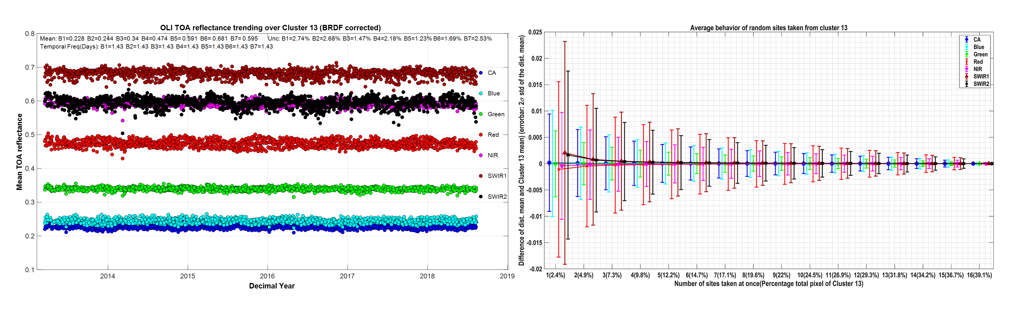
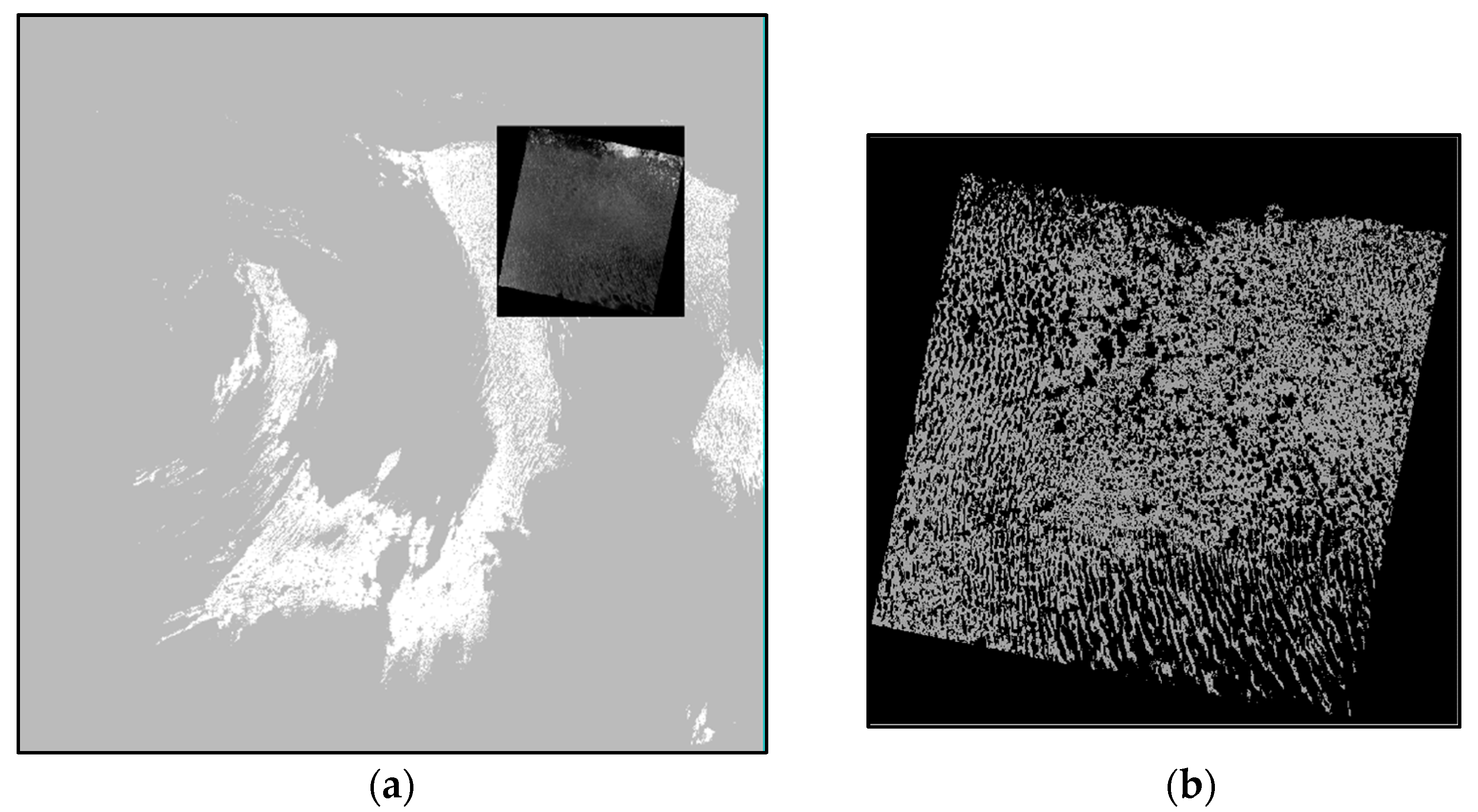
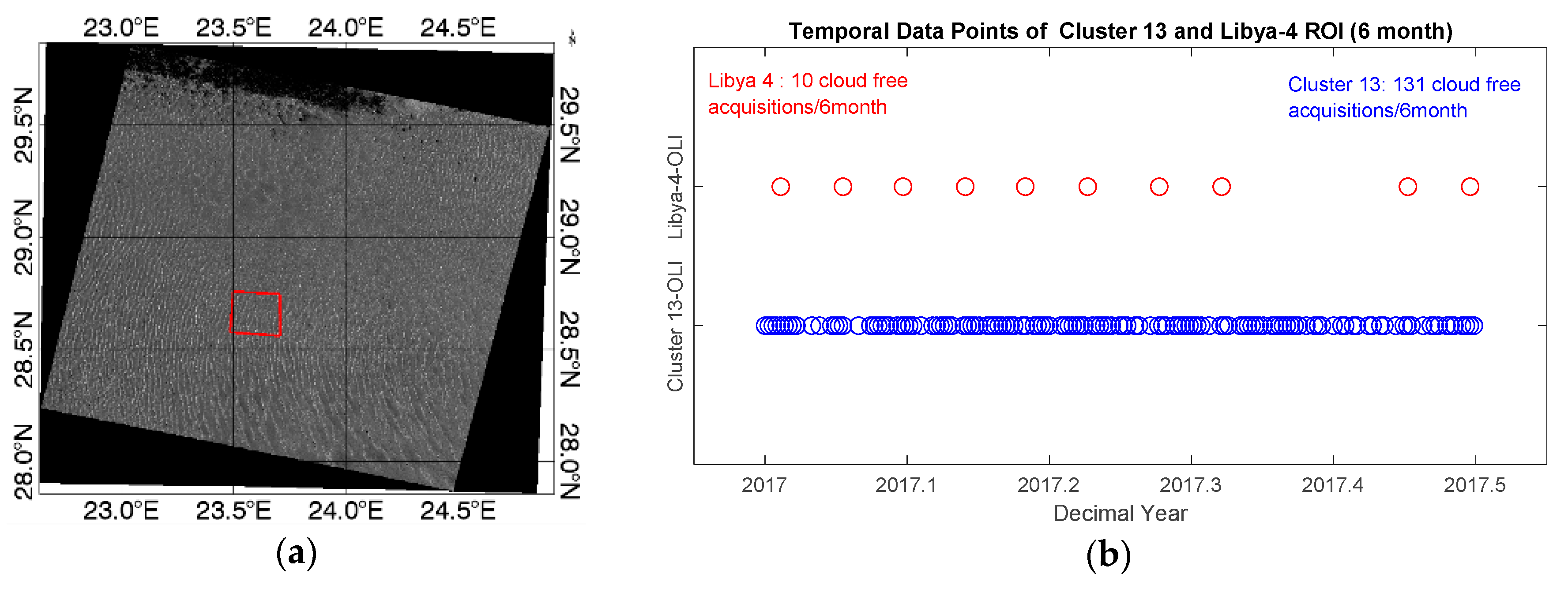
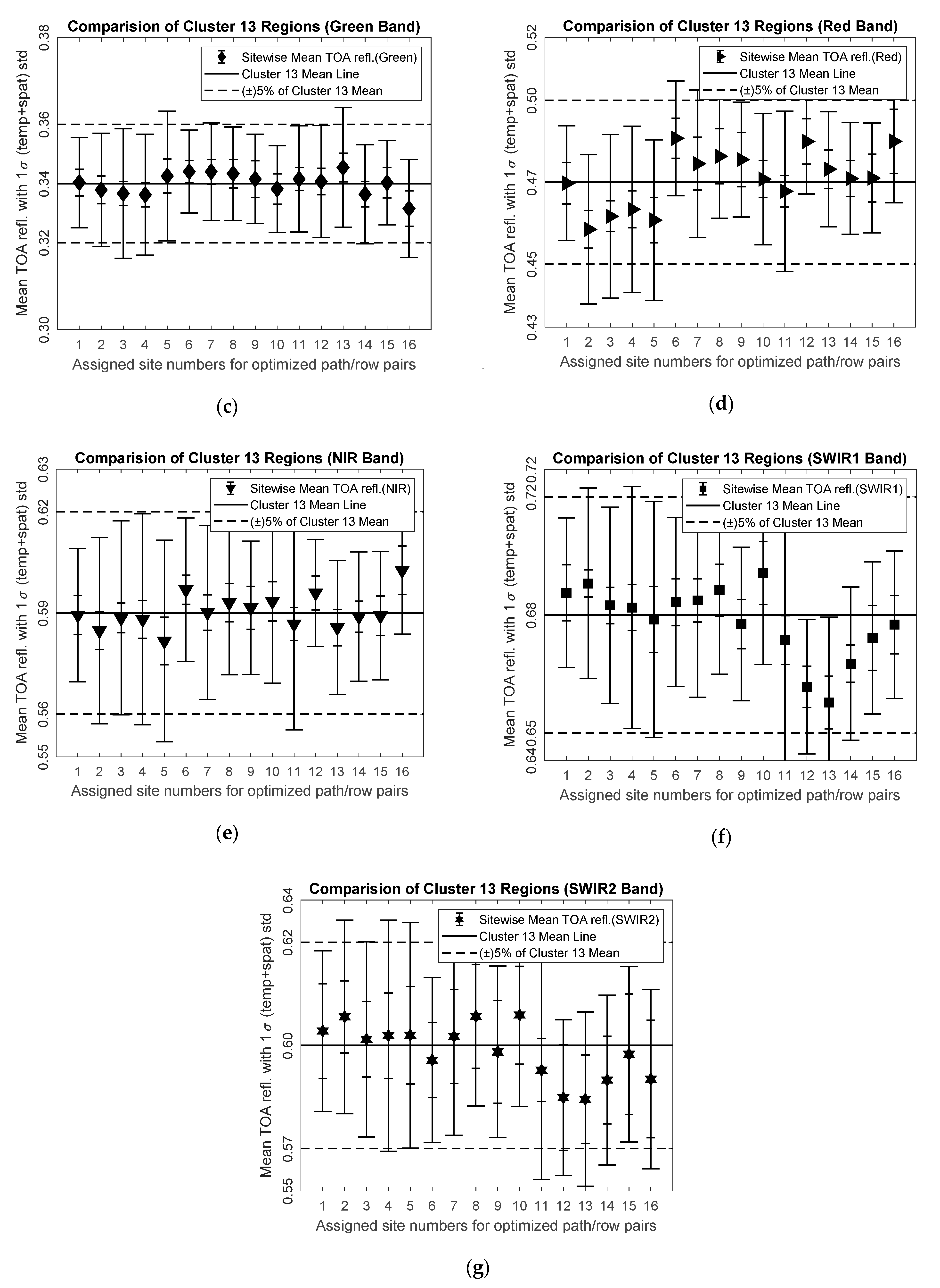
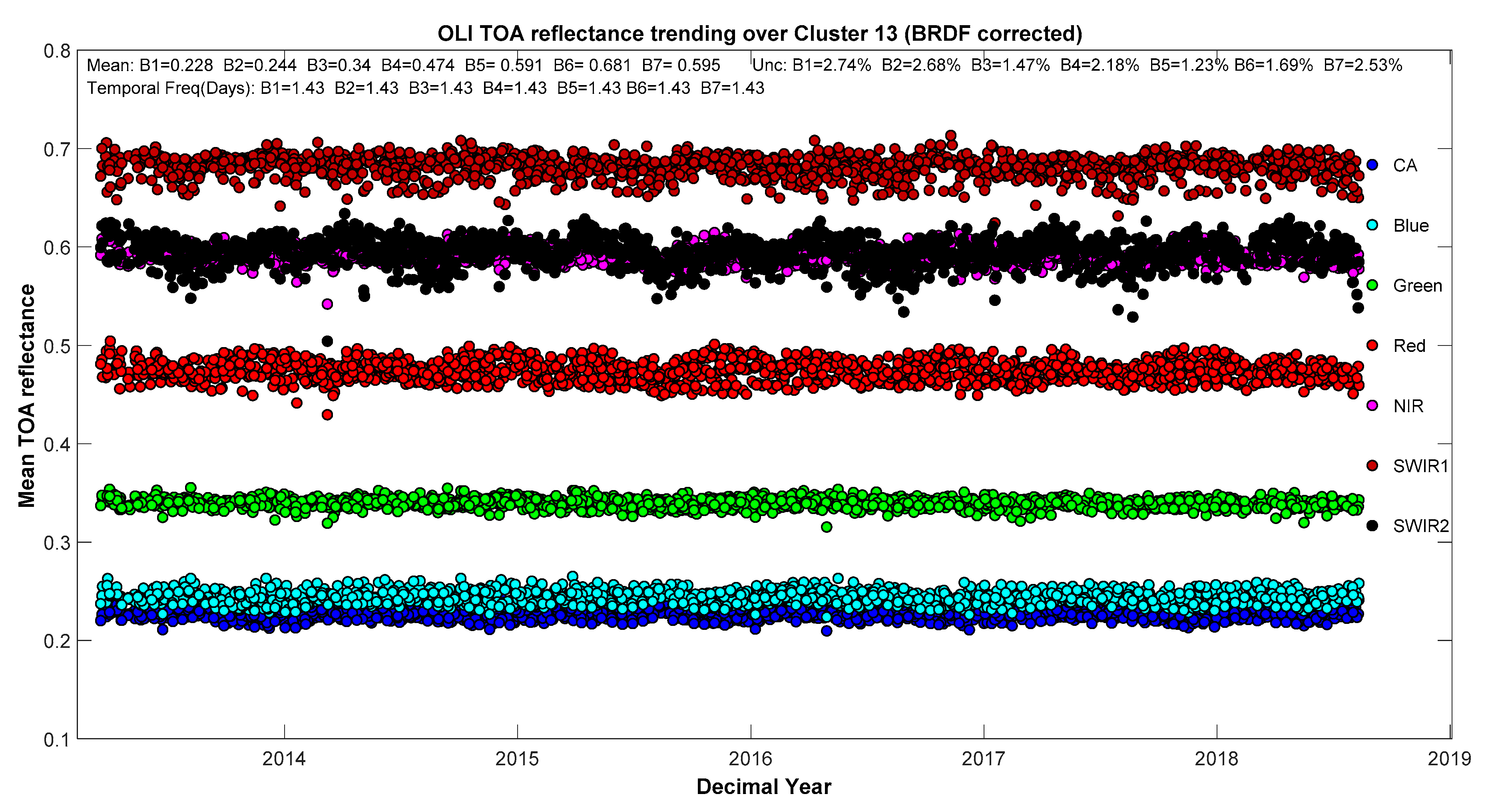
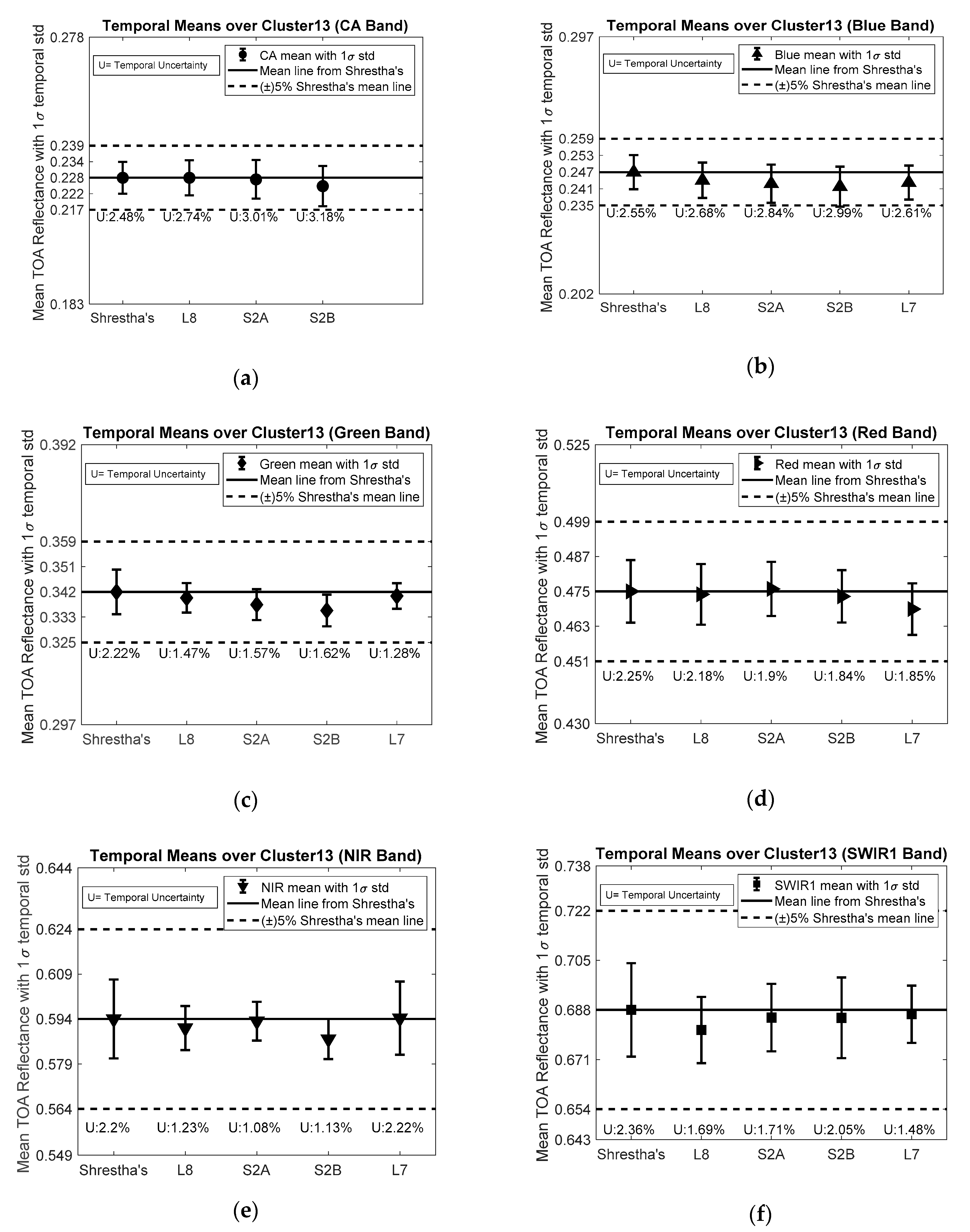
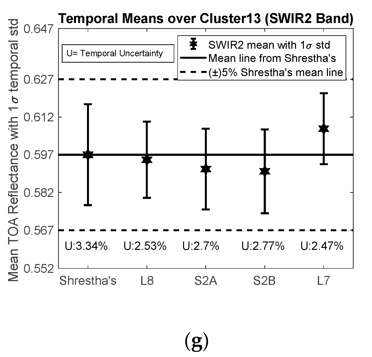
In their paper, Shrestha et al. [17] wanted to identify “optimal” regions that were common across all image bands. They used an unsupervised classification technique to generate a set of 19 classes or “clusters” of spectrally similar OLI image pixels of North Africa based on cloud-free image data filtered for 5% or less temporal uniformity. Each of these clusters can be considered as an “extended” Pseudo Invariant Calibration Site (EPICS). One of the resulting clusters, Cluster 13, was found to possess a spectral response similar to Libya-4, and it contained a significant number of pixels forming relatively large contiguous regions across North Africa; this demonstrated great potential to ensure higher frequency imaging. However, their analysis required downsampling the image data to 300 m spatial resolution, and their results could not be validated with respect to the full resolution image data. In addition, potential BRDF effects were not addressed when generating the spatial and temporal statistics from original cluster data.

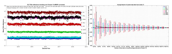
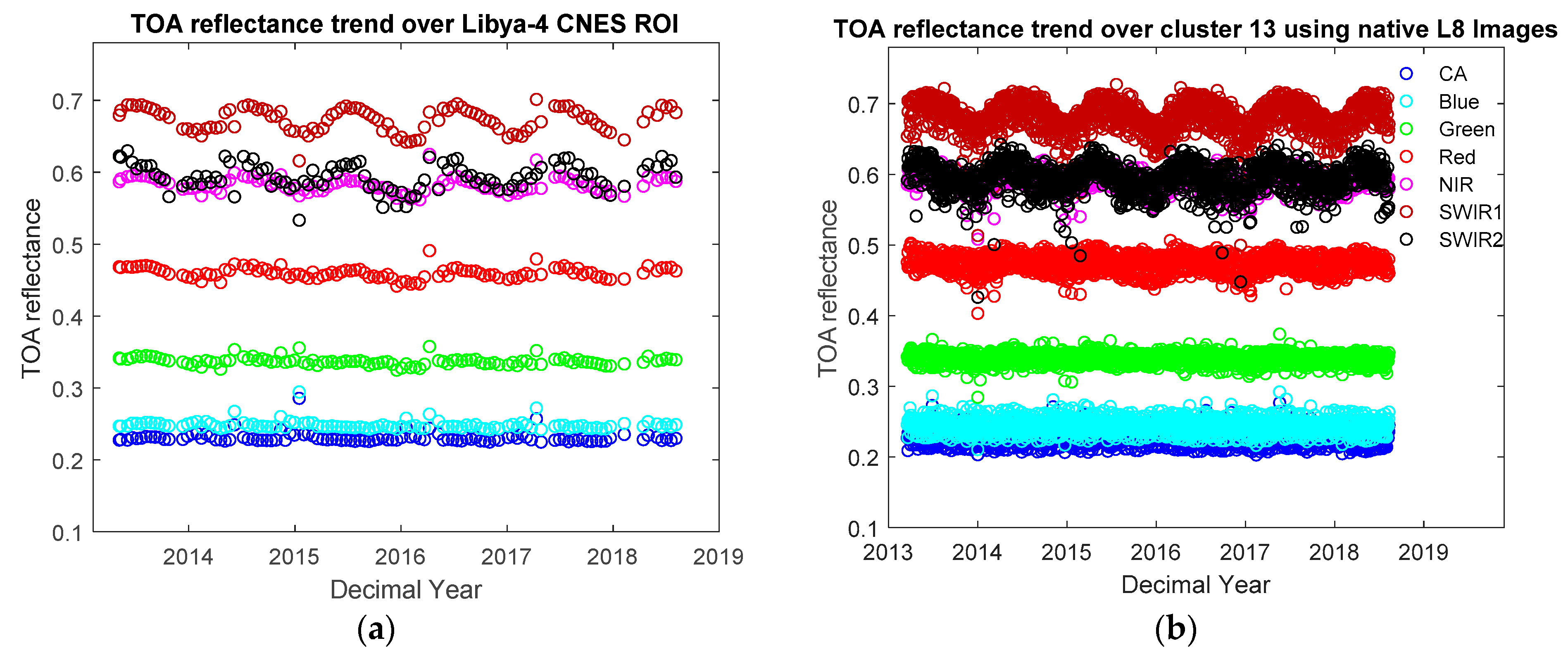
The main purpose of this analysis is to demonstrate the EPICS potential to detect sensor change quicker than traditional PICS via a more temporally rich dataset. Results of this study show that moderate resolution sensors, such as the Landsat 8 OLI, may acquire cloud-free images of Cluster 13 regions once every 1.4 days (using limited and cloud-free scenes only), in contrast to the 18–20 days on average cloud free revisit cycle found over a typical traditional PICS. Although EPICS provided significant improvements in the temporal density of the calibration time series, the resulting analysis showed that the Cluster 13 EPICS exhibited less than 3% uncertainty in its mean temporal TOA reflectance. Using the high density time series, it will be shown that the same period of OLI data over EPICS can provide lower statistically significant minimum detectable trends although Cluster 13 temporal uncertainty is typically found to have uncertainty values which are 1%~2% higher compared to traditional PICS.

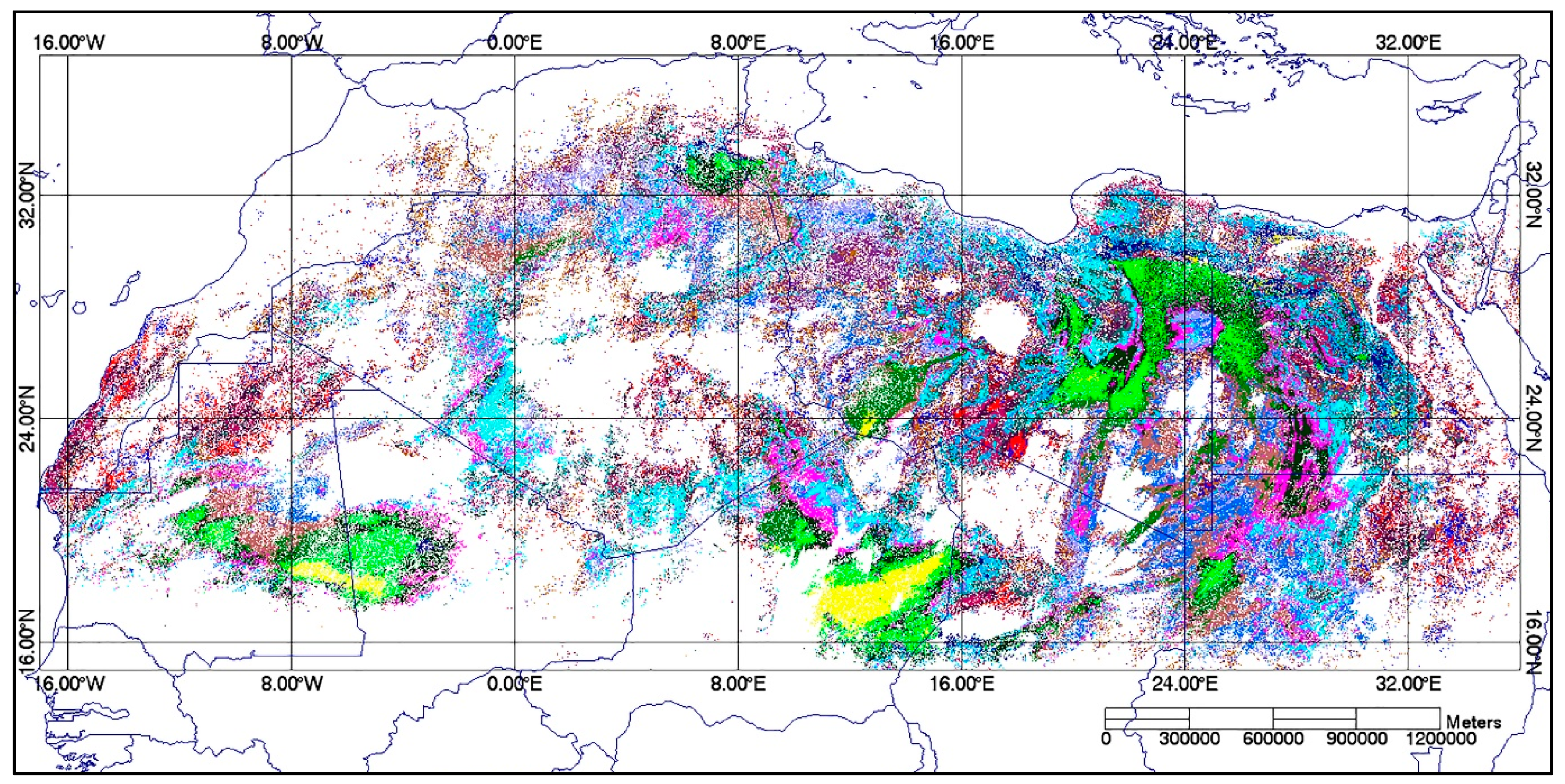
Native Landsat 8 OLI, Landsat 7 ETM+, Sentinel 2A&B MSI image data were used to estimate the overall temporal and spatial variation in radiometric measurements over a major Cluster 13 sub-region (~40% of total area covered by Cluster 13 pixels). In addition, OLI data from Clusters 1, 3, 4, 16, and 19 were analyzed to evaluate sensors across their wider operating dynamic range.

The paper is presented as follows: Section 1 provides a brief review of the topic and previous research performed in this area. Section 2 describes the dataset, mask generation process and application approach in greater detail. Section 3 presents produced results and critical analysis of the results when this process is applied to a number of different sensors. Finally, Section 4 offers some concluding remarks.

2. Methodology

2.1. SDSU Processed Google Earth Engine (GEE) Derived Data and Mosaic of North Africa

In order to develop an EPICS, Shrestha et al. [17] used GEE [18], which utilizes Google’s worldwide processing and storage resources to archive and process freely available image data [19] from Landsat and other satellite sensors, to produce the analysis dataset in their initial stage of work. Inside the GEE environment, OLI was chosen as it has an established calibration accuracy within 3% [10,20]. Temporally filtered and down sampled statistics image datasets (collection of 25 band Image containing the pixel wise temporal mean, temporal standard deviation, temporal uncertainty and the number of valid pixels used to generate those statistics) for the VNIR, SWIR, and Cirrus multispectral bands were retrieved from GEE as 1° latitude by 1° longitude georeferenced chip files. The chips were locally mosaicked into a continental scale, 300 m spatial resolution image of North Africa that covered an area between 36°N to 15°N latitude and 18°W to 35°E longitude. A detailed explanation on the development of the analysis dataset can be found in [17]. This work will take advantage of the already developed EPICS to evaluate its usability for calibration and stability monitoring.

2.2. Classification Map of North Africa

As mentioned in the introduction section, Shrestha’s unsupervised classification algorithm ran on the cloud-screened and temporally filtered mosaic image (mentioned in Section 2.1) identified 19 distinct clusters of spectrally similar surface cover. Figure 1 shows a map of the identified clusters and their distribution throughout North Africa. The bright green pixels represent Cluster 13.

2.3. Cluster 13 as EPICS Candidate Cluster

Shrestha’s original Cluster 13 was found to have an estimated spatial uncertainty (i.e., the ratio of spatial standard deviation to spatial mean of the mosaic filtered pixels) within 3% in all but the Coastal/Aerosol and Blue bands, which had estimated spatial uncertainties within 5%.

Table 1. Mean TOA reflectance and uncertainty of Cluster 13 (Initial analysis found in [17]).

	Bands
	Coastal	Blue	Green	Red	NIR	SWIR1	SWIR2
Mean TOA reflectance	0.23	0.25	0.34	0.48	0.59	0.69	0.60
Average Temporal Uncertainty (%)	2.48	2.55	2.22	2.25	2.20	2.36	3.34
Spatial Uncertainty (%)	4.59	4.8	3.08	2.71	2.11	1.78	2.62

provides the estimated mean TOA reflectance, spatial uncertainty and average temporal uncertainty of Cluster 13 calculated from the 300 m resolution mosaic filtered cluster pixels. Although in the original algorithm the maximum temporal filtering threshold was set at 5%, the unsupervised classification algorithm by Shrestha resulted in less than 3.35% temporal uncertainty across all bands for Cluster 13. The detailed process for determining the uncertainty values will be found in [17]. In addition, Cluster 13 contains a large number of pixels which are aggregated into contiguous regions. Due to its greater degree of pixel aggregation, larger pixel counts, and lower temporal and spatial variability in TOA reflectance measurements, EPICS analyses described in this paper focused on this particular cluster.

2.4. Cluster 13 Boundary Delineation

To create a more portable and easily distributable vector version of the Cluster 13 map, and to make the intermediate process more generic in nature, latitude and longitude coordinates for each Cluster 13 pixel were extracted from the cloud-screened and temporally filtered mosaic image. For the pixels that aggregated together, boundaries where computed, where regions that only contained single pixel were considered too small and filtered out of the remaining process. Then the coordinates for the boundaries were written as polygon vertex coordinates to a Keyhole Markup Language (KML) shape files, through the use of GDAL (Geospatial Data Abstraction Library) software which is released by Open Source Geospatial Foundation [21].

2.5. Creation of Cluster 13 Zone-Specific Masks

To aid and speed up the retrieval of Cluster 13 TOA reflectances from native resolution satellite images, raster masks were created using the boundaries defined in the KML vector file which matched up with the sensor’s specific spatial resolution. The masks where generated at UTM-zone size, which was to improve efficiency of processing. This section describes the mask creation procedure in greater detail.

First, the KML polygon lat/lon coordinates were converted to binary masks whose pixels were registered to the corresponding UTM map projection coordinates; the resulting geo-referenced masks possessed a spatial resolution matching, in this case, the 30 m resolution Landsat images. Images potentially crossing multiple UTM zone boundaries were accounted for by oversizing the mask dimensions by 1.5°, which also resulted in more efficient processing. This procedure is applicable for any sensor as long as the masks are generated to match the sensor’s spatial resolution.

Figure 2 shows two Cluster 13 pixel masks generated with respect to UTM zones 29 and 34, which are shown in grey. The red outlines indicate the cluster region boundaries, the white pixels inside the mask correspond to valid Cluster 13 pixels, and the blue parallelograms represent the footprint of Landsat WRS2 path/rows (considered in additional detail in Section 3). In total, seven masks were needed to represent the entire Cluster 13 region across North Africa, with each mask covering an area of approximately 2,500,000 km².

2.6. Application of Cluster 13 Zone-Specific Masks

The generated Cluster 13 zone specific masks from previous section and quality control/assessment masks (which flags each pixel as clear, clouds, water/snow/ice, fill, etc. and are generally provided with satellite scenes), were applied to each image, and all resultant good pixels were collected. The spatial mean and spatial standard deviation of TOA reflectances were calculated using all the good Cluster 13 pixels of all the scenes available in the local archive (which is a local cache of all good images from Landsat and Sentinel mission, containing less than 5% cloud cover). The process was applied to the all available cloud screened OLI, ETM+, MSI-A (Multispectral Imager of Sentinel 2A), and MSI-B (Multispectral Imager of Sentinel 2B) images. This process created an effective time series of mean TOA reflectance with spatial uncertainties associated with every data point. Temporal mean and temporal uncertainty values were calculated from the time series for evaluation of sensor specific Cluster 13 performance. The average values of corresponding pixel-based sensor view and solar angle geometry were also extracted from each image and stored for later use in BRDF correction. A portion of example UTM zone sized mask (UTM Zone 34) is shown in the bigger frame of Figure 3a where white pixels represent Cluster 13 pixels. The smaller frame overlaid on top of Figure 3a is a Landsat 8 OLI Band 1 scene from WRS-2 Path/Row-181/40. This shows how the UTM zone mask is applied on the satellite imagery. In this case, the Landsat-8 scene is ready to be masked out by the Cluster 13 pixel mask and QA band. Figure 3b shows a filtered TOA reflectance image (magnification applied for better visual representation) for the Coastal/Aerosol band image where the gray level pixels correspond to valid Cluster 13 TOA reflectance pixels.

2.7. Additional Data Filtering

Original Cluster 13 [17] was generated from the filtered 300 m spatial resolution mosaic, with the summary statistics in all input data constrained to a maximum of 5% temporal uncertainty. Table 1 shows that the resulting spatial uncertainties of Cluster 13 across all bands are all within 5%. Consequently, the spatial uncertainty in the native resolution image statistics after application of the georeferenced zonal pixel masks was also expected to be within 5%. So, if an individual data point in a particular band of the Cluster 13 time series dataset exhibited an estimated spatial uncertainty above the 5% threshold, or the data point appeared to deviate significantly from the overall TOA reflectance trend, the corresponding source image was considered “suspect” with respect to clouds/shadows or other conditions not identified in the Quality Assessment (QA) band filtering. The image was then inspected visually; if a previously unidentified cloud/shadow or other artifact was observed, the entire scene’s statistics were excluded from further processing.

2.8. Development of Cluster-Based EPICS BRDF Model

The Cluster 13 time series trends from the different sensors exhibit variability in the TOA measurements, especially in the longer wavelength bands. Several factors can affect this variability including seasonal atmospheric aerosol/water vapor changes. The most significant contributor to this seasonal variation is BRDF effects [22] due mainly to solar position change. The angular dependencies were normalized using the procedure described below.

Image products for the sensors analyzed in this work include information of per-pixel values of the solar and sensor zenith and azimuth angles (For Landsat-8 OLI, per pixel angle band information are in the metadata). Recall from Section 2.6, the georeferenced pixel masks used to generate the Cluster 13 reflectance statistics were also applied to the associated per-pixel angle images to calculate average values for corresponding sensor viewing and solar zenith and azimuth angles. This information was then used to develop a four-angle model which is based on Farhad’s [23] procedure. As the modeling and manipulation of data using computer software (MATLAB) favors the use of Cartesian co-ordinate system and the sensor view and solar angles in the angle band image are given with respect to a three-dimensional spherical coordinate system, the first step in his model generation was to project the angles into a two-dimensional Cartesian coordinate space. Kaewmanee [24] extended Farhad’s linear model with quadratic terms for both solar zenith and solar azimuth angles, including an additional potential interaction term between them. For the purposes of this analysis, Kaewmanee’s approach has been further extended by including all possible interaction terms between the sensor view and solar angles and quadratic terms for the sensor view angles.

A full second-order model was selected to represent a cluster-specific BRDF effect with respect to the transformed zenith and azimuth angles for both solar and view geometries:

$$\begin{gathered} {\rho }_{model}={\beta }_0+{\beta }_1{x}_1+{\beta }_2{y}_1+{\beta }_3{x}_2+{\beta }_4{y}_2+{\beta }_5{x}_1{y}_1+{\beta }_6{x}_1{x}_2+{\beta }_7{x}_1{y}_2+ \\ {\beta }_8{y}_1{x}_2+{\beta }_9{y}_1{y}_2+{\beta }_{10}{x}_2{y}_2+{\beta }_{11}{x}_1^2+{\beta }_{12}{y}_1^2+{\beta }_{13}{x}_2^2+{\beta }_{14}{y}_2^2 \end{gathered}$$

(1)

where ${\rho }_{model}$ is the model predicted TOA reflectance, ${\beta }_{0-14}$ are the model coefficients, and x₁, y₁, x₂, y₂ are the Cartesian coordinates representing the planar projections of the solar and sensor view angles originally given in spherical coordinates:

$$x_1=sin\left(SZA\right)\times cos\left(SAA\right)$$

(2)

$$y_1=sin\left(SZA\right)\times sin\left(SAA\right)$$

(3)

$$x_2=sin\left(VZA\right)\times cos\left(SAA\right)$$

(4)

$$y_2=sin\left(VZA\right)\times sin\left(SAA\right)$$

(5)

where SZA, SAA, VZA, and VAA are the solar zenith/azimuth and sensor viewing zenith and azimuth angles, respectively.

All terms were assumed to be required for effective characterization, as a cluster can contain pixels from widely separated regions possessing distinct, and generally unknown, BRDF characteristics. It has been found that, some terms in the above model presented by Equation (1) becomes insignificant (based on p-values in the regression analysis at 0.05 significance level) which changes from band to band. But, each term in the model equation was significant for at least one band. So, all terms were kept in the model for making the model generic to widely distributed cluster pixels across all bands. The BRDF-normalized TOA reflectance (${\rho }_{BRDF-corrected}$) for each sensor was then determined as follows:

$${\rho }_{BRDF-corrected}=\frac{{\rho }_{obs}}{{\rho }_{model}}\times {\rho }_{ref}$$

(6)

Here, ${\rho }_{obs}$ is the observed mean TOA reflectance from each scene and ${\rho }_{model}$ is the model predicted TOA reflectance. For this analysis,${\rho }_{ref}$ was set to the mean TOA reflectance of the respective time series.

3. Results and Discussion

3.1. Cluster 13 Imaging Frequency

The WRS-2 path/row map and Cluster 13 KML vertex information were overlaid on a Google Earth map of North Africa in order to determine the portions of image data contained within (or “intersecting”) the cluster regions. This information was compared to the Landsat-8 acquisition schedule to determine when the images were acquired within the 16-day revisit period; this provided an estimate of the frequency at which the OLI imaged the cluster. With respect to Landsat-8, 25 WRS-2 paths covered the entire Cluster 13 region, potentially resulting in multiple image acquisitions per day. Thus, this ensures a theoretical better than daily revisit frequency (assuming zero cloudy scenes) of OLI over Cluster 13.

Table 2. Path coverage of Cluster 13 and optimized WRS-2 path/row pairs.

Day of Landsat Cycle	Path Coverage of Cluster 13	Optimized Path/Row	Site Number Assignment	Pixel Count in Million	Area in km2	Additional Path/Row Intersection
1	190	190/43	11	0.50	454	Not Found
2	181,197	181/40	4	17.90	16114	181/41,181/42,181/43,181/48, 197/46,197/47, 197/48
3	188	188/47	9	5.57	5017	188/46, 188/48
4	179	179/41	2	8.39	7548	179/40,179/42,179/44,179/47,179 /48
5	186,202	186/47	7	8.06	7250	186/47,186/48,186/49,202/46,202/47
6	177,193	193/37	14	4.49	4040	177/40,177/41,177/42,177/44, 177/45, 177/46
7	184,200	200/47	16	2.60	2337	184/40, 184/41, 184/42, 184/46, 184/47, 184/49, 200/48
8	191	191/37	12	2.56	2301	Not Found
9	182,198	182/40	5	18.47	16620	182/42,182/43,182/49,198/46,198/47, 198/48
10	189	189/46	10	0.38	339	189/43, 189/44, 189/45,189/47
11	180	180/40	3	7.98	7186	180/41, 180/42, 180/44
12	187,203	187/47	8	9.21	8285	187/42, 187/46, 187/48, 187/49, 203/45, 203/46, 203/47
13	178	178/47	1	8.21	7393	178/40, 178/41, 178/42, 178/43
14	185,201	185/47	6	8.73	7858	185/44, 185/45,185/46,185/48, 185/49, 201/46,201/47
15	192,176	192/37	13	5.55	4999	176/42
16	183,199	199/46	15	5.55	4993	183/40, 183/41,183/42,183/43, 183/49, 199/47,199/48

shows the paths intersecting Cluster 13 on each day of the OLI’s revisit cycle. During days 2, 5, 6, 7, 9, 12, 14, 15, and 16 multiple paths intersect the cluster. In addition, some of the paths have multiple rows intersecting the cluster, which could provide alternate cloud-free acquisitions for a given day and maintain (or even enhance) the temporal resolution of any time series dataset. However, image data from WRS-2 paths 177, 178, 189, and 190 had fewer pixels in their intersecting regions; while these paths might not be considered sufficiently useable for calibration of low resolution sensors, they could still be used for moderate to high resolution sensor calibration. A little deeper look on the table reveals that a total of 87 WRS-2 path/row pairs intersect Cluster 13. Considering no cloud filtering, which is also the best possible case, it can be estimated that the Cluster 13 can be imaged by a moderate resolution sensor with a revisit period of approximately 0.18 (~16/87) day. Again, considering nominal assessments of cloud cover on average 3 out of 10 scenes are rejected, it can then be estimated that Cluster 13 can be imaged by a moderate resolution sensor with a revisit period of 0.33 day (approximately 3 collects per day). This huge improvement of temporal revisit can lead to several important applications such as quicker sensor evaluation, calibration and stability monitoring in a finer scale.

3.2. Cluster Optimization

In order to minimize local processing and storage demands, one WRS-2 path/row pair was selected for each Landsat cycle day, such that the image contained the largest number of Cluster 13 pixels. Based on these criteria, nine paths were excluded from the initial analysis. In addition to the set of useable paths/rows on each cycle day, Table 2 shows the resulting single path/row for each cycle day, the corresponding geographic area (in km²) covered by the path/row image, and the total intersecting Cluster 13 region pixel count. The individual path/rows represent the selected “optimized” path/row (shown in the purple boxes in Figure 2 covering approximately 40% of the total Cluster 13 area). Furthermore, Table 2 shows the additional path/row pairs that could be used if a cloud-free acquisition of the optimized path/row area was not available. In this paper, additional path/rows were not considered due to storage limitation and processing optimization. Table 2 also assigns a site number label to each optimized path/row pairs for flexibility of further use. Starting from East and going through the west of North Africa, ‘site 1’ label is assigned to path/row-178/47 and ‘site 16’ label is assigned to the path/row-200/47. Rest of the optimized path/rows were also assigned site numbers accordingly.

3.3. Traditional PICS vs. EPICS

Figure 4 shows the temporal trend comparison of Cluster 13 (using optimized sites) and Libya-4. A large portion of Libya-4 interests with Cluster 13, therefore it was chosen for this comparison and it is one of the most widely used PICS. For this work, a CNES (National Centre for Space Studies) recommended Libya-4 ROI (70% of the ROI lies within Cluster 13) was used, as shown in Figure 5a. The red rectangle inside the Landsat-8 OLI scene from WRS-2 path/row-181/40 shows the extent of the ROI and the grid values over the Landsat scene gives geographic lat/lon extent of the Landsat scene and the ROI.

The key advantage of cluster-based calibration method is the ability to perform daily/near daily evaluation of a sensor’s stability and calibration. In Figure 4, 1434 cloud-free OLI scenes of Cluster 13 (using optimized path/rows), acquired since launch to August 2018, were used to generate Cluster 13 TOA reflectance time series. The time series reveals that (for the limited data set) Cluster 13 can provide two calibration points in every 3 days (~1.4 per day). But, within the same period, traditional PICS provided only 108 cloud-free scenes generating only 1 calibration point in every 19 days. For better visual observation, the numbers of calibration points were compared between Cluster 13 and Libya 4 in a six-month period as shown in Figure 5b. Libya-4 guaranteed 10 cloud free acquisitions whereas Cluster 13 provided 131 cloud-free scenes in the same time period. This increase (by a factor of approximately 13) in calibration points provides an excellent possibility to detect sensor drift quicker and with more sensitivity than traditional PICS.

Visually from Figure 4, the mean TOA reflectance levels and the temporal variability ranges look very similar. For quantification purpose,

Table 3. Custer 13 vs. Libya-4 temporal and spatial characteristics without BRDF correction.

	Bands	CA	Blue	Green	Red	NIR	SWIR1	SWIR2
Cluster 13 statistics (without BRDF correction)	Mean TOA reflectance	0.228	0.244	0.340	0.474	0.590	0.680	0.594
	Temporal uncertainty (%)	3.07	2.60	1.85	1.88	1.99	2.72	3.29
	Average spatial uncertainty (%)	4.50	4.96	4.35	4.06	4.09	4.00	4.21
Libya-4 ROI statistics (without BRDF correction)	Mean TOA reflectance	0.231	0.248	0.337	0.459	0.582	0.672	0.593
	Temporal uncertainty (%)	3.04	2.56	1.86	1.94	2.02	2.76	3.30
	Average spatial uncertainty (%)	0.68	0.87	1.02	1.09	1.16	1.15	1.17

shows the temporal mean, temporal uncertainty and average spatial uncertainty values associated with Cluster 13 and Libya-4. The relative difference (with respect to Libya-4) between temporal mean of Libya-4 and Cluster 13 ranges from 0.17% (SWIR2) to 3.3% (Red). The temporal uncertainty values associated with the mean values from both Cluster 13 and Libya-4 also do not differ more than 0.01% to 0.06% across all bands. Again, considering the temporal uncertainty values from both Cluster 13 and Libya-4, it can be shown that the mean values for both Cluster 13 and Libya-4 lie within their uncertainty ranges. These similarities imply that the behavior of EPICS is consistent with the behavior of traditional PICS i.e., Libya-4. However, the spatial uncertainty of Cluster 13 is higher than the spatial uncertainty of Libya-4. This is expected as Libya-4 was chosen specifically to reduce variability by finding a “very” homogenous region, where as Cluster 13, allowed for more variation (5% spatial uncertainty criterion that was set in the Shrestha’s classification [17]), in order to achieve greater spatial extent. Some of the extra spatial uncertainties are also due to the variation of solar and view geometry within the individual scenes in the current cluster-based analysis.

3.4. Cluster 13 Region Similarity

Recall that clustering algorithm mentioned in [17] ensured spectral similarity of Cluster 13 pixels to within a temporal and spatial uncertainty of 5% (mentioned in Section 2.3). An analysis was performed to determine whether images from the individual optimized path/rows exhibited similar spectral behavior within the initial uncertainty. For this analysis, cloud-free images of the optimized path/row regions were processed as described in Section 2.6 to determine the summary statistics (temporal mean, temporal uncertainty, and average spatial uncertainty) for the valid Cluster 13 pixels. The TOA reflectance information from each path/row pair for each cycle day was normalized for BRDF effects as described in Section 2.8, then checked to ensure overall spectral similarity to within 5% uncertainty.

Figure 6a–g show the resulting plot of each path/row’s temporal mean reflectances, temporal standard deviations and average spatial standard deviations for all the bands. For the purposes of this analysis, the “site” label on each plot’s horizontal axis is a short-hand notation representing the “optimized” path/row as indicated in Table 2. The estimated temporal standard deviation and total standard deviation due to combined spatial and temporal uncertainty are represented by error bars with smaller and larger caps, respectively. For this analysis, the total uncertainty estimate assumes independence between the temporal and spatial uncertainties:

$$u_{total}=\sqrt{u_{temporal}^2+u_{avg spatial}^2}$$

(7)

where u_total is the propagated uncertainty due to temporal and spatial uncertainty, u_temporal is the temporal uncertainty and u_{avg spatial} is the corresponding mean spatial uncertainty. Figure 6a–g reveal that most of the site’s total standard deviation lies within ±5% of the overall Cluster 13 mean TOA reflectance. However, site 5 in Figure 6a,b and site 12 & 13 in Figure 6f reveal that the deviation of these site’s mean reflectance from Cluster 13 mean is closer to 5%. It means that their contribution to Cluster 13 temporal variability is higher than other sites. This phenomenon suggests that if one of those sites is specifically selected for Cluster 13 behavior estimation, it could underestimate or overestimate the Cluster 13 mean behavior. These relative higher deviations of some site’s mean TOA reflectance compared to Cluster 13 mean raises the question “How many random sites within Cluster 13 are required for calibration and stability assessment of a sensor?” An answer to this question is presented in the next section.

3.5. Expected Behavior of Random Cluster 13 Location

As mentioned earlier, classification algorithm from [17] used to identify the various clusters assumes all data points within a given cluster exhibit the same general spectral behavior. Assuming this spectral similarity, any randomly chosen location within a cluster should, in principle, be able to serve as a source of a representative dataset for the entire cluster. An analysis to test this hypothesis was performed using image data acquired over the 16 sites (recall from Table 2 that “site” is used to indicate the optimized Cluster 13 WRS-2 path/row area imaged on a given cycle day), with the goal of determining the minimum number of sites required to achieve a specified uncertainty in the estimated mean reflectance.

Time series (TS) reflectance datasets, corrected for BRDF effects as described in Section 2.8, were generated for each site. The overall mean TOA reflectance was calculated using all possible distinct combinations of multiple sites (i.e., the overall mean TOA reflectance of the time series for two distinct sites, three distinct sites etc). 16 individual time series’ were created separately for 16 optimized sites where each time series has a distinct temporal mean TOA reflectance value. From this pool of 16 “temporal mean” values for “16 optimized sites”, first, one site combination was considered which produced ¹⁶C₁ = 16 different combinations. Similarly, two site combination produced ¹⁶C₂ = 120 combinations and three site combinations produced ¹⁶C₃ = 560. This process was repeated for rest of the combinations up to 16 sites considering at once which created ¹⁶C₁₆ = 1 combination (this combination is essentially the representative of Cluster 13 considered here). The generic formula used here is the combination formula i.e., ⁿC_r where n is number of “temporal mean values” in the pool and r is the number of “sites/time series considered at once”. For each possible time series combination, the mean TOA reflectance was calculated. Distribution of mean TOA reflectance’s was then constructed from the individual time series combination means, as shown in Figure 7, where combinations of two distinct sites are presented as an example.

For further example, Figure 8a,b present the distribution of reflectance means for the Coastal/Aerosol band. In this case, eight distinct sites providing 12870(¹⁶C₈) distinct means and three distinct sites generating 560(¹⁶C₃) distinct means were used to create the sampling distributions. The mean values and standard deviations of the distributions are represented by a solid circular symbol and associated horizontal error-bars respectively. In Figure 8a where eight sites were considered at once, the mean of the distribution is 0.2275 and 1 sigma standard deviation is 0.0012 which produces an uncertainty (standard deviation divided by mean value) of 0.5363%. Again, looking at the Cluster 13 temporal mean for this band (~0.2276) suggests that this distribution can predict Cluster 13 mean TOA reflectance within 0.0439% of Cluster 13 mean and with an associated uncertainty of 0.5363%. Similarly, Figure 8b suggests that using only three sites will give a prediction of same TOA reflectance but with a higher uncertainty value of 1.11% (distribution mean = 0.2275, standard deviation = 0.0025). Taking all the site combinations, looking at the distribution means of all bands and comparing with cluster mean values, it has been observed that the reduction in uncertainty is exponential with the increase of number of sites used to estimate Cluster 13 behavior.

Figure 9 shows the estimated reflectance difference (i.e., distribution mean—Cluster 13 mean) for all bands, as a function of the number of distinct sites used to calculate the distribution mean. The numbers inside the parentheses at the horizontal axis label gives an average pixel count used by the considered number of sites.

The error-bars represent the estimated standard deviation of the distribution means. As might be expected, using more distinct sites to represent the entire Cluster 13 region tends to decrease the uncertainty in the estimated reflectance mean. The envelope created by each band’s standard deviation bars tend to decrease exponentially with the increasing number of sites, meaning that increasing the number of sites increases the likelihood of reaching the Cluster 13 TOA reflectance level in an exponential manner. Looking at the 3-site combination in x-axis of Figure 9, the absolute differences for all bands tend to reach zero and the distribution standard deviations are all within ±0.01 reflectance unit. This case is mentioned in the previous paragraph which produces an uncertainty of ~1%. It suggests that prediction of the Cluster 13 TOA reflectance’s within 1% uncertainty is possible using only three sites. Again, from

Table 4. Distribution mean and uncertainty for worst case scenario (single location).

	CA	Blue	Green	Red	NIR	SWIR1	SWIR2
Distribution mean	0.227	0.244	0.34	0.475	0.591	0.68	0.593
Distribution uncertainty (%)	2.03	2.07	0.92	1.75	0.86	1.56	1.34

, it is predictable that using single site will provide the highest uncertainty (the worst-case scenario) which is around 2% across coastal and blue bands. All these results suggest that the Cluster 13 mean TOA reflectance can be estimated within an uncertainty of maximum 2% using only one site and within 1% uncertainty using only three sites leaving a choice to trade-off between accuracy and number of sites selection.

3.6. Validation

As mentioned in the Introduction section, Shrestha’s original clusters were generated from the GEE derived Landsat OLI dataset which- (i) lacked BRDF correction for Sun and sensor geometry variations; and (ii) required down sampling the original image data to 300 m resolution, so Cluster 13 temporal trending was evaluated using OLI, Landsat-7 ETM+, and Sentinel 2A/2B MSI image data at their native spatial resolutions, including BRDF correction as needed. Figure 10 shows the cluster-level temporal trend for all OLI bands after applying the BRDF correction described in Section 2.8.

The corresponding statistics are presented in

Table 5. Mean OLI (L8) TOA reflectance of Cluster 13 optimized path/rows by band, derived from 30 m image data.

	Bands
	CA	Blue	Green	Red	NIR	SWIR1	SWIR2
Mean TOA reflectance	0.228	0.244	0.340	0.474	0.591	0.681	0.595
Temporal Uncertainty (%)	2.74	2.68	1.47	2.18	1.23	1.69	2.53
Average Spatial Uncertainty (%)	4.50	4.96	4.35	4.06	4.09	4.00	4.21

. Additionally, temporal mean values, temporal uncertainty values and temporal revisit intervals are also mentioned at the top portion of the figure. The temporal uncertainties of Cluster 13 lie within 3% across all the bands which suggests that Cluster 13 is as stable as traditional PICS sites while offering much larger ROI which also results in minimal infuse for any specific localized land change or variability. Some of the bands such as Green, NIR, and SWIR1 bands are extremely stable—less than 1.5%. Again, some seasonality is still left in the SWIR2 channel producing relatively higher temporal uncertainty compared to its nearby longer wavelength bands which needs to be further investigated. Overall, temporal uncertainties from the optimized path/row pairs are less than the Cluster 13 temporal uncertainties predicted from [17] (also shown in Table 1) except for Coastal/Aerosol and Blue bands. This reduction in uncertainty values was expected because the BRDF effects in longer wavelengths were minimized in the trending showed in Figure 10 whereas corresponding values from [17] lacked this compensation.

The dataset for classification of North Africa was derived using Landsat 8 OLI images. So, Sentinel 2A MSI, Sentinel 2B MSI, and Landsat 7 ETM+ were used for independent validation of the Cluster 13 reflectance statistics. Sentinel 2A MSI and Sentinel 2B MSI image tiles were selected such that a significant portion of the optimized WRS2 path/rows were included within it, as listed in

Table 6. Path/row images (OLI, ETM+) and tile images (MSI-A, MSI-B) used for validation.

Optimized Path/Row Pairs with Respect to OLI	Optimized Path/Row Pairs Used for Validation with Respect to ETM+	Optimized Sentinel 2A/2B MSI Tile ID	Optimized Path/Row Pairs with Respect to OLI	Optimized Path/Row Pairs Used for Validation with Respect to ETM+	Sentinel 2A/2B MSI Tile ID
200/47	Not Used	29QNA	187/47	Same as OLI	32QRF
199/46	Not Used	29QRC	186/47	Same as OLI	33QUA
193/37	Not Used	32SKB	185/47	Same as OLI	33QWA
192/37	Not Used	32SLB	182/40	Same as OLI	34RFT
191/37	Not Used	32SMB	181/40	Same as OLI	34RGS
190/43	Not Used	32QNM	180/40	Same as OLI	35RLN
189/46	Same as OLI	32QPH	179/41	Same as OLI	35RMK
188/47	Not Used	32QPG	178/47	Same as OLI	35QLA

. Similarly, Landsat 7 ETM+ scenes were also selected by optimizing its intersection with Cluster 13 (i.e., same as OLI). But, only nine path/rows of Landsat 7 ETM+ were selected due to data storage limitations. The spectral differences between the Landsat OLI, Sentinel 2A MSI, Sentinel 2B MSI, and Landsat 7 ETM+ were compensated by applying spectral adjustment factor (SBAF) to Sentinel and Landsat 7 data sets. The SBAF correction process can be found in [25]. This compensation was done to ensure a better comparison between the Cluster 13 TOA reflectance measurements from different sensors.

Figure 11 compares the estimated temporal means and associated standard deviations between initial Cluster 13 temporal statistics from [17] and Cluster 13 temporal statistics derived from Landsat 8 OLI, Sentinel 2A MSI, Sentinel 2B MSI, and Landsat 7 ETM+. The results shown here assume common bands across all sensors; the ETM+ does not have a corresponding Coastal/Aerosol band. The common bands across Landsat OLI and Sentinel 2A and 2B MSI bands can be found in [26]. The mean TOA reflectance from Shrestha’s initial Cluster 13 analysis is represented by the black solid line and its 5% uncertainty range is represented by the dashed black line as shown in Figure 11. Additionally, temporal uncertainty associated with each measurement is also mentioned at the bottom of each sensor’s measurement. Looking at the four different sensors, they behave consistently across all the bands. The temporal mean values are all within their uncertainties. Uncertainty values of Coastal/Aerosol and Blue band are around 3% across all sensors, which are mostly due to atmospheric scattering. Green, Red, NIR and SWIR1 channels show ~2% (or less) uncertainty compared to the original uncertainty ranges mentioned in [17]. The comparing sensors produce less uncertainty values in these bands due to application of BRDF correction. Again, compared to their longer wavelength counterparts, SWIR2 channel uncertainty values were little higher (close to 3%) due to their water vapor absorption feature which was not properly characterized and corrected. However, the estimated temporal uncertainties associated with the TOA reflectance measurements were all within ±3% in all bands across all sensors which imply that Cluster 13 temporal behavior is similar irrespective to the different sensors.

3.7. Extension of Dynamic Range Using Lower Reflectance Clusters

The 19 clusters from Shrestha’s analysis have their own distinct spectral signatures which provide a wide dynamic range for sensor calibration especially at longer wavelengths as shown in Figure 12.

Cluster 2 and Cluster 4 are the brightest and darkest respectively. A brief analysis of Cluster 1, 3, 4, 16, and 19 was done in order to increase the dynamic range of cluster-based sensor calibration. The detailed analysis of all the clusters is out of the scope of this paper. From these selected clusters, the temporal trend of the darkest cluster, Cluster 4, is presented in Figure 13. The Figure shows that the reflectance levels are in between 0.177 and 0.38 for all bands.

Table 7. Mean TOA Reflectance with Standard Deviation and Uncertainty of Cluster 4 optimized path/rows by band, derived from 30 m image data.

Bands	CA	Blue	Green	Red	NIR	SWIR1	SWIR2
Mean	0.181	0.177	0.204	0.262	0.314	0.380	0.326
Temporal Standard Deviation	0.0112	0.0130	0.0155	0.0157	0.0118	0.0145	0.0122
Temporal Uncertainty (%)	6.2%	7.35%	7.59%	5.97%	3.76%	3.82%	3.75%

summarizes mean TOA reflectances with standard deviation and uncertainty of Cluster 4 optimized path/rows by band, derived from OLI data. Despite being the darkest cluster, it has temporal uncertainty less than 8% for visible bands and even better uncertainty, i.e., less than 5%, for the infrared bands. Because of having lower signal levels from this cluster, the relative uncertainty measure might not reflect the true impression of the behavior of this dark cluster as dividing the standard deviation by a very small mean TOA reflectance values tend to produce a larger uncertainty value. So, absolute standard deviation numbers were also included in the Table for a better understanding of this cluster’s behavior. It reveals that the standard deviation values are in between around 0.011~0.016 which are assumed to be relatively low considering this cluster is darkest one and found in the desert. So, despite being the darkest cluster across North Africa, Cluster 4 can also be considered as a stable EPICS and can be used for calibration purposes.

It has been observed that not only all the found clusters are widely distributed across North Africa, but also they are temporally and spatially stable which makes them eligible for stability monitoring of satellite sensors over a wide dynamic range. For optimizing data storage, only 16 paths and rows of Cluster 4 were used. Using those 16 path/row pairs, Cluster 4 can be observed approximately twice in 3 days. However, if all the path/row pairs are used to their full potential, this cluster can also be observed more than once a day. It means that this cluster has also daily or near daily calibration opportunity. Another interesting fact about the found clusters is that, some path/row pairs include more than one cluster regions within their single; For example, path/row 176/46 and 185/42 contain regions of Cluster 1, 3, 16, and 19 which can be very useful for calibrating the sensors that image limited regions of the Earth only. This allows such type of sensors to look at a single location and calibrate for a wider dynamic range.

3.8. Increase of Sensitivity to Detect Change in the Sensor

This section describes how the temporally rich dataset from Cluster 13 can help to detect “sensor change” quicker than traditional PICS. Due to the harsh environment in space, sensor response often decays with time and the reflectance trend starts to produce nonzero slope. Because of temporal variability present in the time series, the magnitude of the slope needs to exceed a certain minimum value, which is determined by computing the statistically significant minimum detectable trend.

The following equation in Weatherhead et al. [27,28] allows estimation of the required number of years (N) to detect a trend of magnitude $m$ at the 95% confidence level and with 50% probability:

$$\mathrm{N}={\left(\frac{2{\mathsf{\sigma }}_N}{\left|m\right|}\sqrt{\frac{1+\varnothing }{1-\varnothing }}\right)}^{2/3}$$

(8)

where, ${\mathsf{\sigma }}_N$ is month-to-month variability and $\varnothing$ is the 1-month lag autocorrelation in the time series. This equation can also be used to estimate minimum detectable trend when N (in years) is given as input. However, it was necessary to make sure that the units of ${\mathsf{\sigma }}_N$ and $m$ are the same in the equation.

Using this equation, Bhat et al. [11] found that the minimum detectable trend values are of the order 1%~3% while using Libya-4 data. Their study was conducted on VIIRS visible & SWIR band observations limited from February 2013 to October 2013.

For this paper, minimum detectable trends for both a one year period and the total period of the analysis data (Launch-August 2018; total 5.39 years) were estimated using the Equation (8). To comply with the equation requirements, the original TOA reflectance time series (both Cluster 13 and Libya-4) were converted to monthly observations by averaging the BRDF corrected TOA reflectance’s over each month. As mentioned in [27,28], ${\mathsf{\sigma }}_N$ in the above equation was expressed as month to month variability (in percentage) by dividing the overall standard deviation of the monthly averaged TOA reflectance’s by the overall mean values. Similarly, N is computed in terms of years by dividing the total number of months by 12. One-month lag autocorrelation coefficient calculation process is described as following.

Autocorrelation (also known as serial correlation) is a statistical method which is widely used in time series analysis to detect non randomness in a dataset by measuring the correlation of a signal with a delayed copy of itself. It is often expressed as a function (autocorrelation function) of the time lag between the two copies of signal. Mathematically, the autocorrelation function measures the correlation between $y_t$ and $y_{t+k}$, where k = 0, 1, 2, ..., K are time lags and$y_t$ is a stochastic process. According to [29], the autocorrelation $r_k$ for lag k is:

$$r_k=\frac{c_k}{c_0}$$

(9)

where, $c_k$ is the estimate of the autocovariance and $c_0$ is the sample variance defined as

$$c_k=\frac{1}{N}{{\displaystyle \sum }}_{t=1}^{N-k}\left(y_t-\overline{y}\right)\left(y_{t+k}-\overline{y}\right)$$

(10)

$$c_0=\frac{1}{N}{{\displaystyle \sum }}_{t=1}^N{\left(y_t-\overline{y}\right)}^2$$

(11)

In the above equations $\overline{y}$ is the the sample mean of the time series defined as:

$$\overline{y}=\frac{1}{N}{{\displaystyle \sum }}_{t=1}^N{y}_t$$

(12)

and, N is the number of observations present. As both Cluster 13 and Libya-4 time series is converted to a monthly sampled time series, the autocorrelation at lag k = 1 is the one-month lag autocorrelation.

Table 8. Estimated minimum detectable trend comparison between EPICS and traditional PICS.

	Bands	CA	Blue	Green	Red	NIR	SWIR1	SWIR2
Minimum detectable trend of OLI (%/yr)	1 year—Libya-4	3.62	4.01	3.17	3.77	2.77	2.04	4.65
	1 year—Cluster 13	2.31	2.50	1.33	2.33	1.36	1.65	4.28
	5.4 years—Libya-4	0.29	0.32	0.25	0.30	0.22	0.16	0.37
	5.4 years—Cluster 13	0.18	0.20	0.11	0.19	0.11	0.13	0.34

shows minimum detectable trends of OLI for both EPICS and traditional PICS. For every band the cluster-based approach produced a lower amount of minimum detectable trends. For example, when 1-year observation data from both Libya-4 and Cluster 13 is available, Libya-4 produced a minimum detectable trend value of 3.17%/yr in Green band while Cluster 13 produced a value of 1.33%. This is a substantial increase of sensitivity in drift detection. However, the minimum detectable trend values of SWIR2 band shows less improvement compared to other bands. It is more likely due to uncompensated seasonal noise present in this channel. Estimated minimum detectable trend for full time frame (5.4 years) from Table 8 reveals that although the observation years were increased to 5.4 times, the decrease in minimum detectable trend is around 12 times. The exponential increase of the sensitivity of drift detection with the time can be attributed to the Equation (8) which depends on natural variability, autocorrelation and observation period of the time series dataset.

Although Cluster 13 (16 path/row limited) temporal variabilities are on the order of 2.7% and Libya-4 CNES uncertainties are of 1% (except SWIR2~2%), the increase of temporal density allowed the Cluster-based method to produce more sensitivity in sensor change detection. However, due to autocorrelation in both Cluster 13 and Libya-4 datasets the minimum detectable trend often produces larger values indicating that one might have to wait for several years to detect even a unit percentage of change in the sensor performance using PICS/EPICS based approach. For example, it has been found that an unit percent change in Coastal Aerosol band can be detected in 2.35 years using Libya-4 data whereas Cluster 13 can detect the same change in 1.74 years; This values decreases to 1.22 years (Cluster 13) and 1.97 years (Libya-4) for NIR band due to less temporal variations present in the BRDF corrected dataset. A similar decrease is also observed for green channel.

Table 9. Trend detection time improvement by EPICS compared to Libya-4.

	CA	Blue	Green	Red	NIR	SWIR1	SWIR2
Time required(years) for Cluster-13 to detect 1 year equivalent Libya-4 trend	0.74	0.73	0.56	0.72	0.62	0.86	0.96
Time required(years) for Cluster-13 to detect 5.4 years equivalent Libya-4 trend	3.99	3.94	3.02	3.91	3.36	4.67	5.01

shows the estimate of time required using Cluster 13 to detect the same amount of minimum trend estimated from OLI data over Libya-4 CNES ROI. It shows that the limited Cluster-13 can detect the same amount of trend in about half a year faster (Green band) compared to Libya 4 CNES ROI (1 year time frame). Referring to Figure 10, it is visible that the temporal trend of green band after BRDF correction has very less temporal variation while the SWIR2 channel has the largest variations. As the Equation (8) used to calculate minimum detectable trend also depends on the variability of time series, Green band takes less amount of time and the SWIR2 channel shows less improvement using Cluster based method.

4. Summary and Conclusions

This paper focuses on the application of EPICS (Cluster) for stability monitoring of optical satellite sensors. EPICS provides a significant improvement of the temporal revisit period of calibration time series in contrast to the temporal revisit period offered by traditional PICS with similar or 1%~2% higher temporal uncertainties depending on bands. One of the clusters, Cluster 13 (using limited regions and cloud-free scenes only), offers temporal revisit period of potentially as good as 1.4 days for Landsat 8 OLI in contrast to an average of every 18–20 days obtained from traditional PICS. By using all the regions of Cluster 13 and a nominal cloud consideration (~around 30% scene rejection due to cloud cover) a temporal revisit period of 0.33 day (~three cloud free collects everyday) can be obtained by a moderate resolution sensor. Furthermore, for the sensors having a wide field of view, Cluster 13 can offer even less than this revisit period. This improvement in the temporal revisit period resulted in better (depending on bands the increase in sensitivity as large as ~2 times) sensitivity of drift detection.

The temporal uncertainty of Cluster 13 was analyzed and validated using Landsat 8 OLI, Landsat 7 ETM+, Sentinel 2A MSI, and Sentinel 2B MSI. All sensors agree that Cluster 13 is temporally stable within 3%. However, spatial uncertainty of Cluster 13 is around 5% which is slightly more variation than that of traditional PICS. This extra spatial variation is pronounced due to its large spatial extent across the continent. Even though Cluster 13 with its hugely extended target size has spatial uncertainty of 5%, still the goal of matching traditional PICS temporal uncertainty is achieved. The near daily/daily calibration opportunity and increased sensitivity of change detection outweighs traditional PICS based methods, while also reducing the impact of a single location “change”.

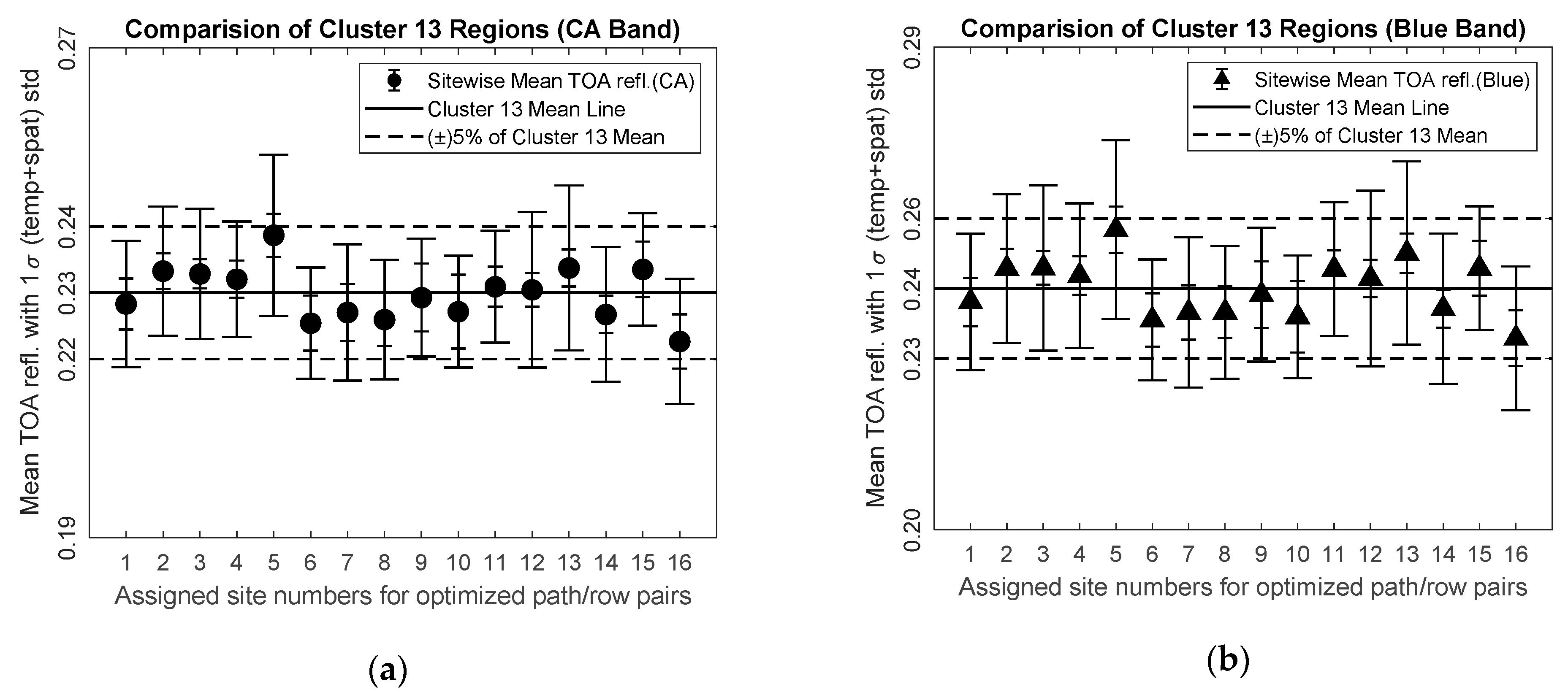
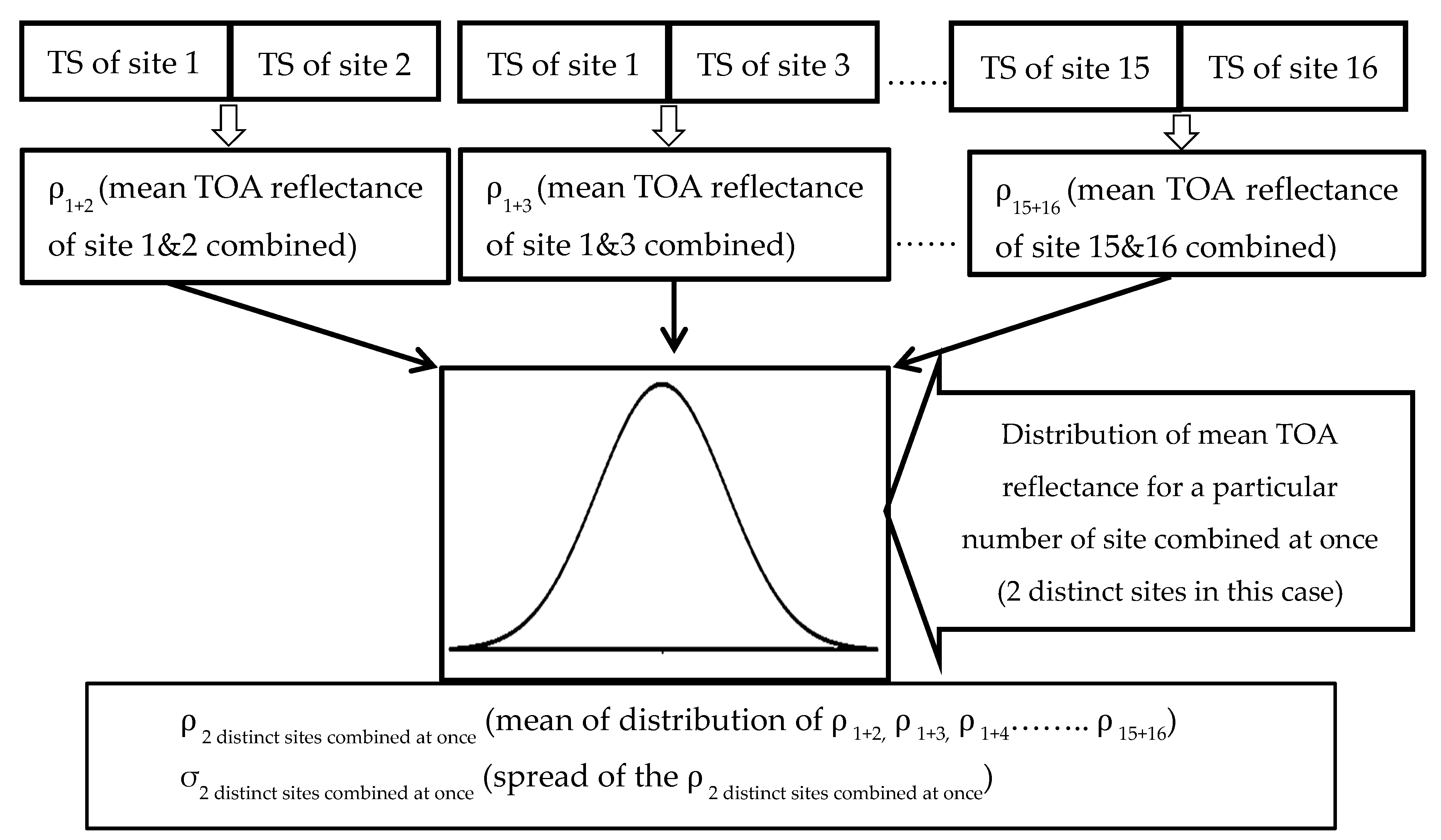
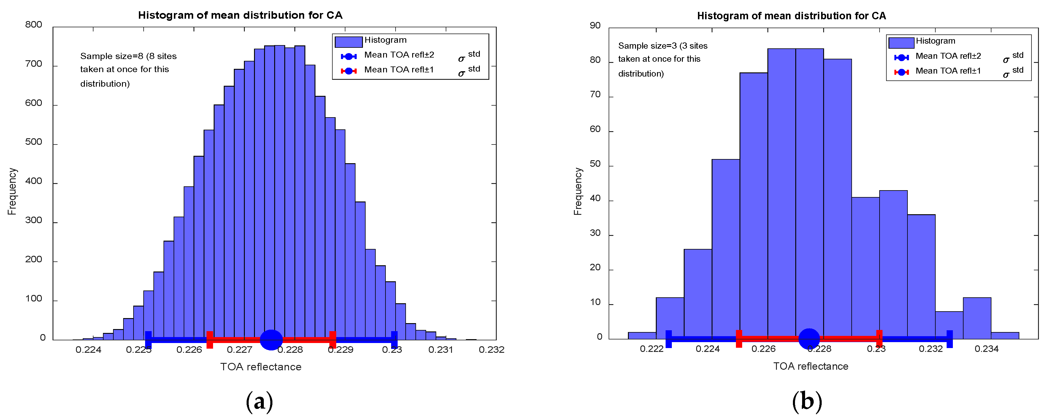
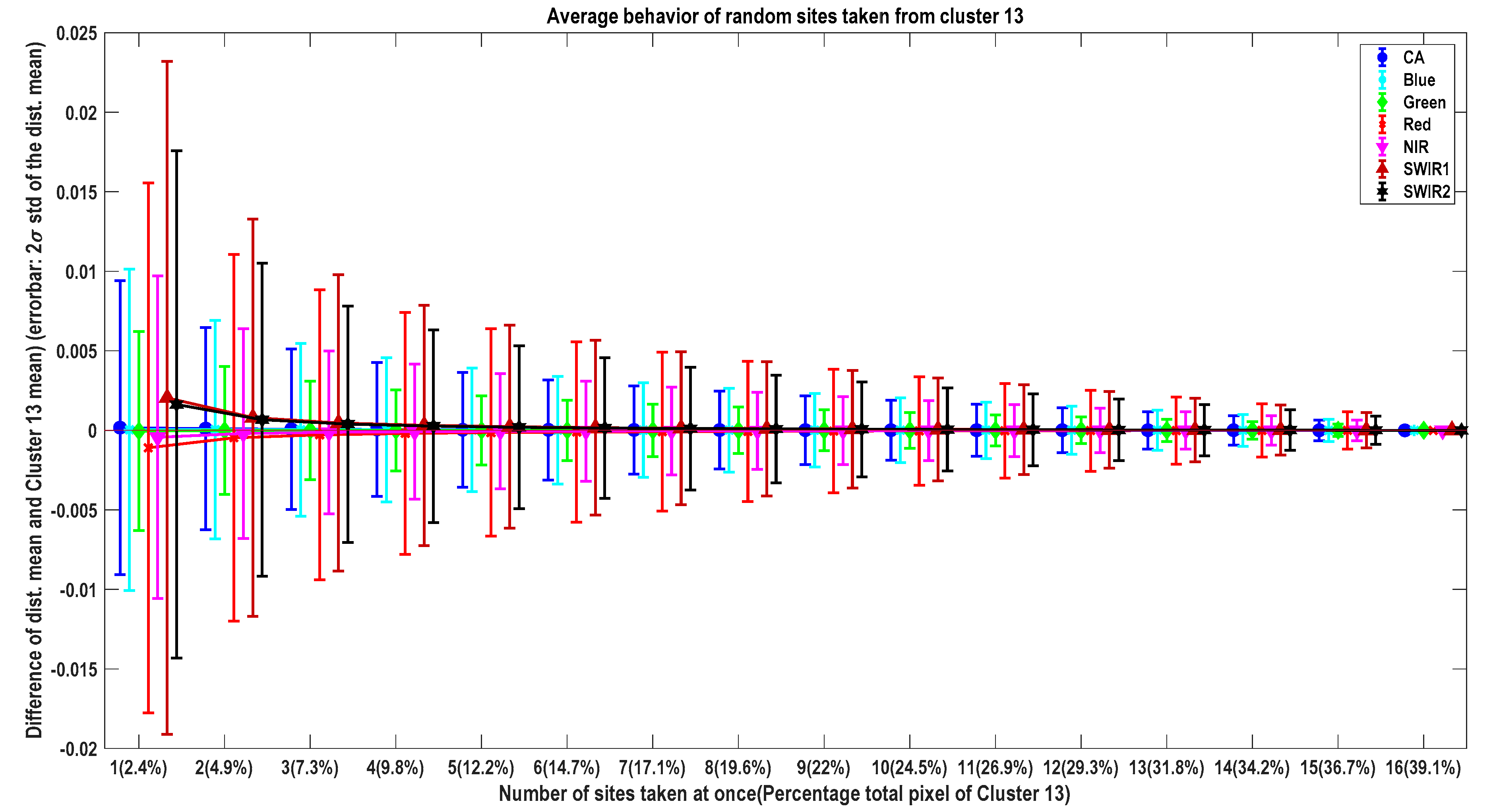
This paper also suggests that a single random location from Cluster 13 can be a representative of the whole Cluster 13 with 2% uncertainty. This uncertainty value becomes smaller exponentially with the increase of chosen locations. A typical decrease of uncertainty values to 1% using only 3 sites has been observed while mean values estimated by 3 sites differs no more than 0.0439% of Cluster 13 mean TOA reflectance values. This suggests that the Cluster 13 mean TOA reflectance can be estimated within a specified uncertainty using fewer number of sites that is tunable to achieve desired accuracy.

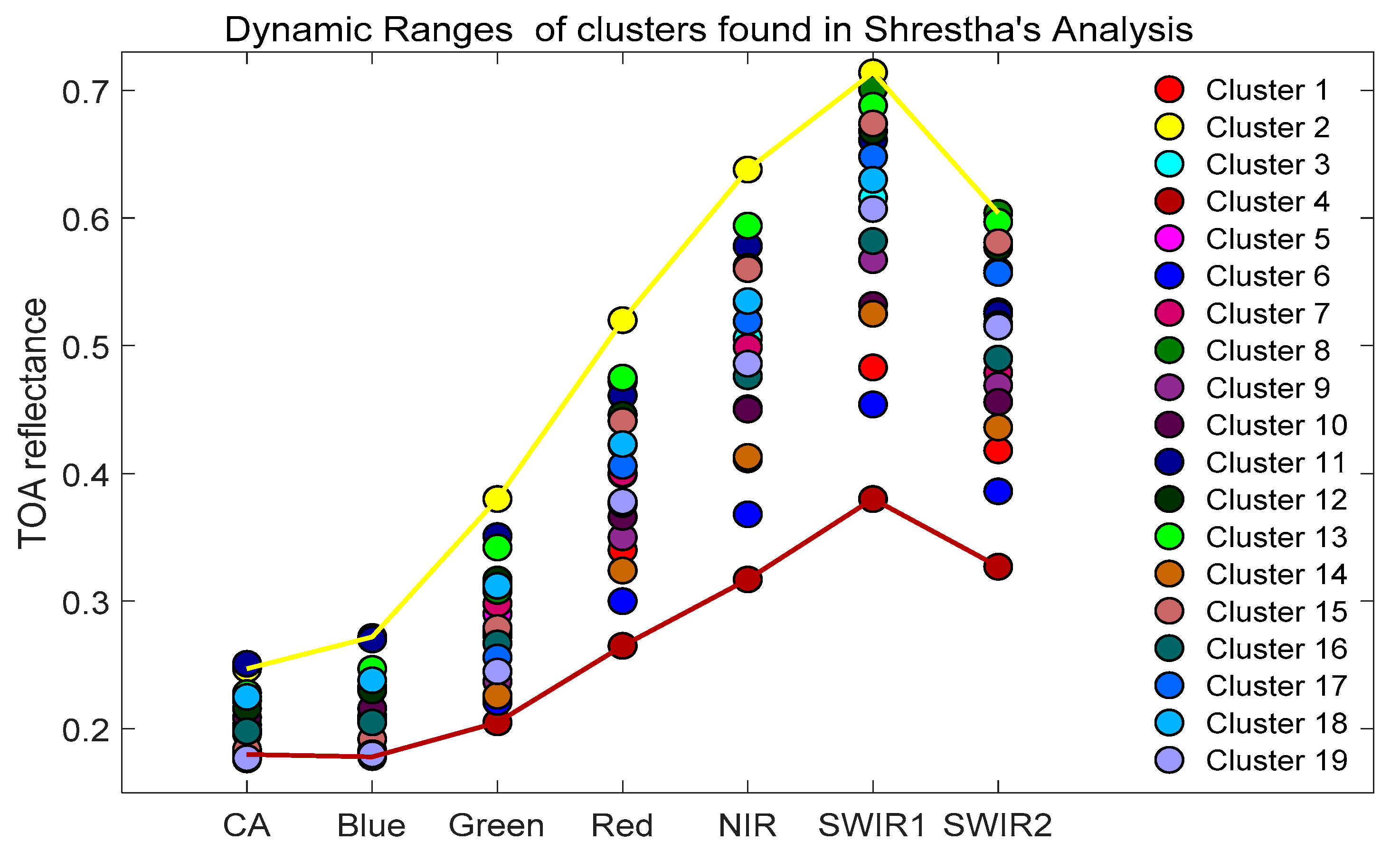
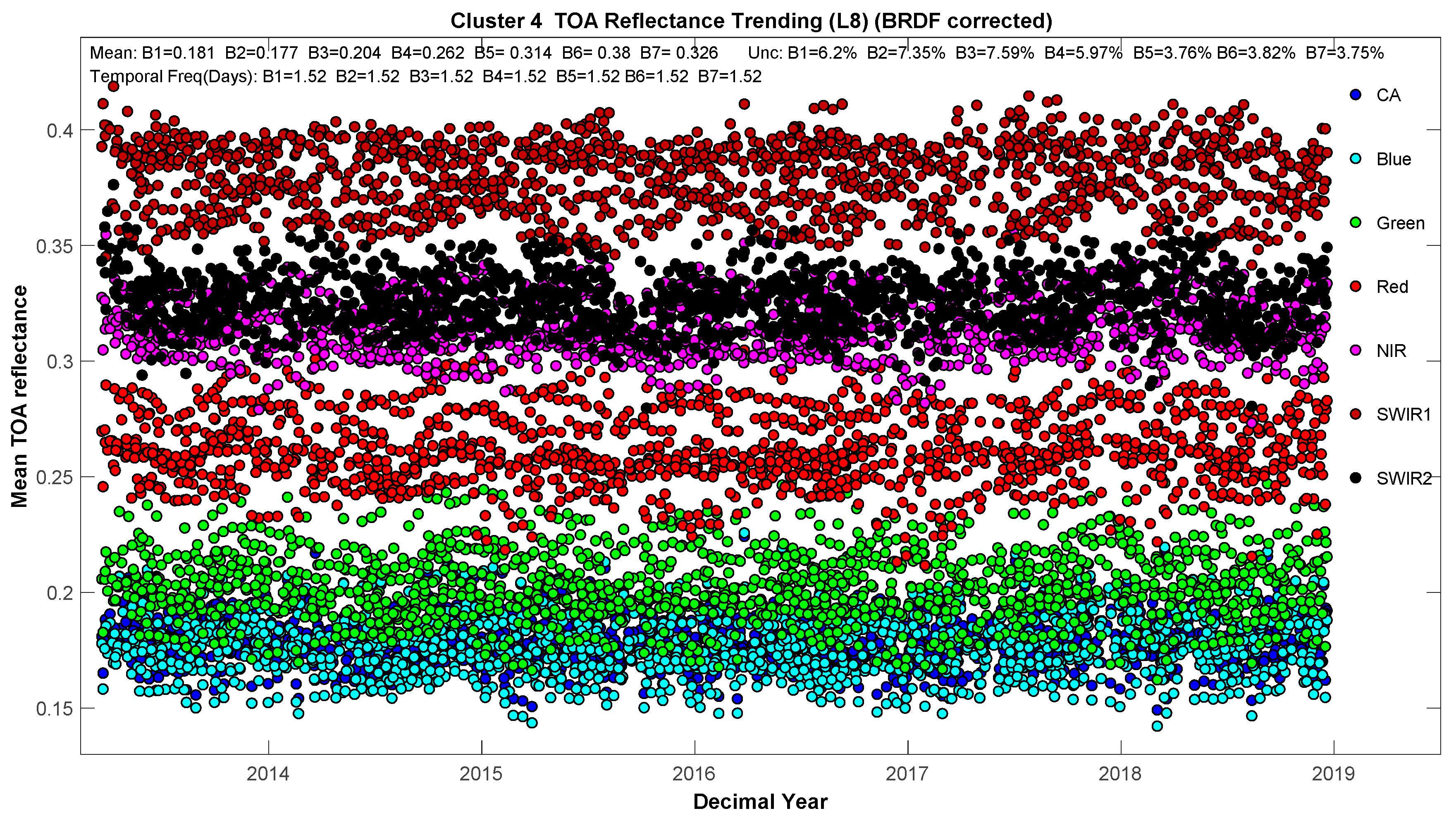
The analysis in this work is more focused on Cluster 13 as it has better spatial uncertainty across all the bands and widely distributed across North Africa. But there are other clusters, such as Cluster 1, 3, 4, 16, and 19, which have spatial uncertainty and distribution across North Africa comparable with Cluster 13. Initial results showed that these clusters also offer nearly daily acquisition as Cluster 13. These clusters possess a similar potential to be used for EPICS based sensor calibration within their specified uncertainty. The darkest of the found clusters, Cluster 4 has temporal TOA reflectance mean values ranging from 0.177–0.380 with absolute standard deviation values ranging from 0.011~0.0016. This generates temporal uncertainty values ranging from 5%~8% which are the highest values among the considered clusters and can be useful for calibration purposes considering the intensity level of this cluster. Furthermore, these clusters have different intensity levels which can help to perform radiometric calibration and stability monitoring of any satellite sensors in a wider dynamic range.

This paper showed that EPICS allows daily or near daily calibration and stability monitoring. EPICS offers up to two times (this number varies from band to band) better sensitivity in drift estimation than traditional PICS even with its continental extent. The proposed technique can be powerful for evaluating sensor performance in less time, especially for sensors with shorter lifespans and limited spatial coverage. Surprisingly, EPICS achieves all this improvement while offering less than 3% temporal variability in its reflectance time series.

References

1. Cabot, F.; Hagolle, O.; Henry, P. Relative and multitemporal calibration of AVHRR, SeaWiFS, and VEGETATION using POLDER characterization of desert sites. In Proceedings of the IGARSS 2000, IEEE 2000 International Geoscience and Remote Sensing Symposium, Taking the Pulse of the Planet: The Role of Remote Sensing in Managing the Environment, Proceedings (Cat. No. 00CH37120), Honolulu, HI, USA, 24–28 July 2000; pp. 2188–2190. [Google Scholar]
2. Cosnefroy, H.; Leroy, M.; Briottet, X. Selection and characterization of Saharan and Arabian desert sites for the calibration of optical satellite sensors. Remote Sens. Environ. 1996, 58, 101–114. [Google Scholar] [CrossRef]
3. Kaufman, Y.; Holben, B. Calibration of the AVHRR visible and near-IR bands by atmospheric scattering, ocean glint and desert reflection. Int. J. Remote Sens. 1993, 14, 21–52. [Google Scholar] [CrossRef]
4. Kim, W.; He, T.; Wang, D.; Cao, C.; Liang, S. Assessment of long-term sensor radiometric degradation using time series analysis. IEEE Trans. Geosci. Remote Sens. 2014, 52, 2960–2976. [Google Scholar] [CrossRef]
5. Teillet, P.; Barsi, J.; Chander, G.; Thome, K. Prime candidate earth targets for the post-launch radiometric calibration of space-based optical imaging instruments. In Proceedings of the Earth Observing Systems XII, San Diego, CA, USA, 5 October 2007; p. 66770S. [Google Scholar]
6. Teillet, P.; Chander, G. Terrestrial reference standard sites for postlaunch sensor calibration. Can. J. Remote Sens. 2010, 36, 437–450. [Google Scholar] [CrossRef]
7. Wu, A.; Zhonc, Q. A method for determining the sensor degradation rates of NOAA AVHRR channels 1 and 2. J. Appl. Meteorol. 1994, 33, 118–122. [Google Scholar] [CrossRef]
8. Chander, G.; Xiong, X.J.; Choi, T.J.; Angal, A. Monitoring on-orbit calibration stability of the Terra MODIS and Landsat 7 ETM+ sensors using pseudo-invariant test sites. Remote Sens. Environ. 2010, 114, 925–939. [Google Scholar] [CrossRef]
9. Markham, B.L.; Thome, K.J.; Barsi, J.A.; Kaita, E.; Helder, D.L.; Barker, J.L.; Scaramuzza, P.L. Landsat-7 ETM+on-orbit reflective-band radiometric stability and absolute calibration. IEEE Trans. Geosci. Remote Sens. 2004, 42, 2810–2820. [Google Scholar] [CrossRef]
10. Markham, B.; Barsi, J.; Kvaran, G.; Ong, L.; Kaita, E.; Biggar, S.; Czapla-Myers, J.; Mishra, N.; Helder, D. Landsat-8 operational land imager radiometric calibration and stability. Remote Sens. 2014, 6, 12275–12308. [Google Scholar] [CrossRef]
11. Bhatt, R.; Doelling, D.; Wu, A.; Xiong, X.; Scarino, B.; Haney, C.; Gopalan, A. Initial stability assessment of S-NPP VIIRS reflective solar band calibration using invariant desert and deep convective cloud targets. Remote Sens. 2014, 6, 2809–2826. [Google Scholar] [CrossRef]
12. Wu, A.; Xiong, X.; Cao, C.; Chiang, K.-F. Assessment of SNPP VIIRS VIS/NIR radiometric calibration stability using Aqua MODIS and invariant surface targets. IEEE Trans. Geosci. Remote Sens. 2016, 54, 2918–2924. [Google Scholar] [CrossRef]
13. Angal, A.; Chander, G.; Xiong, X.; Choi, T.J.; Wu, A. Characterization of the Sonoran desert as a radiometric calibration target for Earth observing sensors. J. Appl. Remote Sens. 2011, 5, 059502. [Google Scholar] [CrossRef] [Green Version]
14. Angal, A.; Xiong, X.; Choi, T.; Chander, G.; Wu, A. Using the Sonoran and Libyan Desert test sites to monitor the temporal stability of reflective solar bands for Landsat 7 enhanced thematic mapper plus and Terra moderate resolution imaging spectroradiometer sensors. J. Appl. Remote Sens. 2010, 4, 043525. [Google Scholar]
15. Tabassum, R. Worldwide Optimal PICS Search; South Dakota State University: Brookings, SD, USA, 2017. [Google Scholar]
16. Vuppula, H. Normalization of Pseudo-Invariant Calibration Sites for Increasing the Temporal Resolution and Long-Term Trending; South Dakota State University: Brookings, SD, USA, 2017. [Google Scholar]
17. Shrestha, M.; Leigh, L.; Helder, D. Classification of North Africa for Use as an Extended Pseudo Invariant Calibration Sites (EPICS) for Radiometric Calibration and Stability Monitoring of Optical Satellite Sensors. Remote Sens. 2019, 11, 875. [Google Scholar] [CrossRef]
18. Gorelick, N.; Hancher, M.; Dixon, M.; Ilyushchenko, S.; Thau, D.; Moore, R. Google Earth Engine: Planetary-scale geospatial analysis for everyone. Remote Sens. Environ. 2017, 202, 18–27. [Google Scholar] [CrossRef]
19. Woodcock, C.E.; Allen, R.; Anderson, M.; Belward, A.; Bindschadler, R.; Cohen, W.; Gao, F.; Goward, S.N.; Helder, D.; Helmer, E. Free access to Landsat imagery. Science 2008, 320, 1011. [Google Scholar] [CrossRef] [PubMed]
20. Knight, E.; Kvaran, G. Landsat-8 operational land imager design, characterization and performance. Remote Sens. 2014, 6, 10286–10305. [Google Scholar] [CrossRef]
21. GD Team. GDAL—Geospatial Data Abstraction Library. 2013. Available online: http://www.gdal.org (accessed on 10 May 2019).
22. Roujean, J.L.; Leroy, M.; Deschamps, P.Y. A bidirectional reflectance model of the Earth’s surface for the correction of remote sensing data. J. Geophys. Res. Atmos. 1992, 97, 20455–20468. [Google Scholar] [CrossRef]
23. Farhad, M. Cross Calibration and Validation of Landsat 8 OLI and Sentinel 2A MSI; South Dakota State University: Brookings, SD, USA, 2018. [Google Scholar]
24. Kaewmanee, M. Pseudo Invariant Calibration Sites: PICS Evolution; Utah State University: Logan, UT, USA, 2018. [Google Scholar]
25. Chander, G.; Mishra, N.; Helder, D.L.; Aaron, D.B.; Angal, A.; Choi, T.; Xiong, X.; Doelling, D.R. Applications of spectral band adjustment factors (SBAF) for cross-calibration. IEEE Trans. Geosci. Remote Sens. 2013, 51, 1267–1281. [Google Scholar] [CrossRef]
26. Zhang, H.K.; Roy, D.P.; Yan, L.; Li, Z.; Huang, H.; Vermote, E.; Skakun, S.; Roger, J.-C. Characterization of Sentinel-2A and Landsat-8 top of atmosphere, surface, and nadir BRDF adjusted reflectance and NDVI differences. Remote Sens. Environ. 2018, 215, 482–494. [Google Scholar] [CrossRef]
27. Weatherhead, E.C.; Reinsel, G.C.; Tiao, G.C.; Jackman, C.H.; Bishop, L.; Frith, S.M.H.; DeLuisi, J.; Keller, T.; Oltmans, S.J.; Fleming, E.L. Detecting the recovery of total column ozone. J. Geophys. Res. Atmos. 2000, 105, 22201–22210. [Google Scholar] [CrossRef] [Green Version]
28. Weatherhead, E.C.; Reinsel, G.C.; Tiao, G.C.; Meng, X.L.; Choi, D.; Cheang, W.K.; Keller, T.; DeLuisi, J.; Wuebbles, D.J.; Kerr, J.B. Factors affecting the detection of trends: Statistical considerations and applications to environmental data. J. Geophys. Res. Atmos. 1998, 103, 17149–17161. [Google Scholar] [CrossRef]
29. Box, G.E.; Jenkins, G.M.; Reinsel, G.C.; Ljung, G.M. Time Series Analysis: Forecasting and Control, 5th ed.; John Wiley and Sons: Hoboken, NJ, USA, 2015; ISBN 978-1-118-67502-1. [Google Scholar]
Figure 1. North Africa cluster map.
Remotesensing 11 01755 g001
Figure 2. Cluster 13 pixel masks for UTM zones 29 (shaded region on left) and 34 (shaded region on right).
Remotesensing 11 01755 g002
Figure 3. (a) Portion of Cluster 13 pixel mask overlaid on OLI Image (UTM Zone 34, WRS-2 Path/Row 181/40) (Left); (b) Masked TOA reflectance image, Coastal/Aerosol band (Right).
Remotesensing 11 01755 g003
Figure 4. TOA reflectance trend from (a) Libya-4 ROI (Left); (b) Cluster 13 without any further cloud screening and correction (Right).
Remotesensing 11 01755 g004
Figure 5. (a) Libya-4 CNES ROI (Red rectangle) over WRS-2 path-row 181/40 image from Landsat 8 (Left). (b) Improvement of temporal revisit period using EPICS over traditional Libya-4 PICS (Right).
Remotesensing 11 01755 g005
Figure 6. Mean temporal TOA reflectance values (with associated total standard deviations) of 16 individual Cluster 13 WRS-2 Path/Row(s): (a) CA band; (b) Blue band; (c) Green band; (d) Red band; (e) NIR band; (f) SWIR1 band; (g) SWIR2 band .
Remotesensing 11 01755 g006aRemotesensing 11 01755 g006b
Figure 7. Procedure to create analysis dataset for determining expected behavior of random Cluster 13 location.
Remotesensing 11 01755 g007
Figure 8. Histogram of the mean distribution of CA band when (a) eight distinct sites were considered at once (Left) and (b) three distinct sites were considered at once (Right).
Remotesensing 11 01755 g008
Figure 9. Average expected behavior of randomly selected site from Cluster 13.
Remotesensing 11 01755 g009
Figure 10. OLI lifetime TOA reflectance trend of Cluster 13.
Remotesensing 11 01755 g010
Figure 11. Validation of Cluster 13 mean temporal TOA reflectance values using OLI, Sentinel 2A/2B MSI, and ETM+ Sensors: (a) CA band; (b) Blue band; (c) Green band; (d) Red band; (e) NIR band; (f) SWIR1 band; (g) SWIR2 band.
Remotesensing 11 01755 g011aRemotesensing 11 01755 g011b
Figure 12. Dynamic ranges of clusters found by Shrestha’s analysis.
Remotesensing 11 01755 g012
Figure 13. Temporal trending of OLI over Cluster 4.
Remotesensing 11 01755 g013