A Novel Hyperspectral Endmember Extraction Algorithm Based on Online Robust Dictionary Learning

Abstract

Due to the sparsity of hyperspectral images, the dictionary learning framework has been applied in hyperspectral endmember extraction. However, current endmember extraction methods based on dictionary learning are not robust enough in noisy environments. To solve this problem, this paper proposes a novel endmember extraction approach based on online robust dictionary learning, termed EEORDL. Because of the large scale of the hyperspectral image (HSI) data, an online scheme is introduced to reduce the computational time of dictionary learning. In the proposed algorithm, a new form of the objective function is introduced into the dictionary learning process to improve the robustness for noisy HSI data. The experimental results, conducted with both synthetic and real-world hyperspectral datasets, illustrate that the proposed EEORDL outperforms the state-of-the-art approaches under different signal-to-noise ratio (SNR) conditions, especially for high-level noise.

1. Introduction

Due to the complexity of natural ground spectra and the low spatial resolution of the remote-sensing hyperspectral imaging process, pixels of these images are by nature, mixtures of several spectral signatures known as endmembers [1]. This mixing is problematic for the downstream processing of hyperspectral images (HSIs) and for applying such methods in real-world scenarios, including target detection [2], classification [3] and change detection [4]. In many application scenarios such as target detection, a certain level of subpixel accuracy is required in order to improve the image processing output, which means that unmixing the HSIs is crucial. In most cases, the endmember spectral signatures of HSIs are not known in advance. Thus, the hyperspectral unmixing process must be performed in an unsupervised way, which usually involves two steps, namely, endmember extraction and abundance estimation. Endmember extraction is the key step in the decomposition of mixed pixels, that is, the determination of the basic features of the mixed pixels in the observed image, the result of which greatly affects the accuracy of the estimation of the abundance coefficients. Therefore, endmember extraction is of great significance in spectral unmixing.

There are two types of mainstream spectral mixing analysis models—the linear mixing model (LMM) and the nonlinear mixing model (NLMM) [5,6,7]. The LMM regards each mixed pixel as a linear combination of several endmember spectral signatures weighted by their corresponding abundance coefficients. Considering the physical meaning of the abundance coefficient, the value of abundance should satisfy non-negativity. Because of its simplicity and effectiveness, the LMM is more widely used in endmember extraction than the NLMM [8,9]. In this paper, it is assumed that the mixed pixels follow the LMM.

Endmember extraction for HSIs has become a popular research topic in recent years, and numerous algorithms have been proposed to crack the barriers in HSI processing. Existing algorithms can be classified into two groups: pure pixel-based algorithms and non-pure pixel-based algorithms.

The methods based on the pure pixel hypothesis assume that the image contains at least one pure pixel corresponding to each endmember and look for the vertexes of the convex simple volume as the endmembers that constitute a given image. Representative algorithms include the pixel purity index (PPI) [10], vertex component Analysis (VCA) [11], N-FINDR [12], the automatic target generation process (ATGP) [13], the simplex growing algorithm (SGA) [14] and so on. These kinds of algorithms generally have low computational complexity and high efficiency, and can obtain good endmember extraction results when the observed image satisfies the pure pixel assumption. However, in a real situation, the pure pixel assumption is often difficult to satisfy.

Many endmember extraction algorithms based on the non-pure pixel hypothesis have been proposed for highly mixed HSI data. Convex geometry-based algorithms are most widely used; these are based on the assumption that a convex simplex contains all observation data points and finds the endmembers through minimizing the simplex volume. Representative algorithms include minimum volume simplex analysis (MVSA) [15], minimum volume constrained non-negative matrix factorization (MVC-NMF) [16], robust collaborative NMF (RCoNMF) [17] and so on. Also, because the results obtained by a single convex model are often not good enough, the piecewise convex multiple-model endmember detection algorithm (PCOMMEND) was proposed in [18]. The model, which is based on the multiple convex region assumption is better able to describe the spectral variability in HSIs.

In addition to the aforementioned convex geometry-based endmember extraction algorithms, methods based on dictionary learning have received extensive attention from scholars worldwide because of the similarity of the basic mathematical models. Now, dictionary learning-based endmember extraction approaches have become a popular research topic. A spectral unmixing method based on sparse dictionary learning is proposed in [19], which obtains good results in the observed image reconstruction. However, this approach requires quite a high signal to noise ratio (SNR). With regard to dictionary learning theory, an endmember extraction algorithm based on online dictionary learning (EEODL) has been proposed [20]. This method reduces the computational complexity by using the online scheme and it performs well with highly mixed images, although it is still somewhat sensitive to noise. Thus, an untied denoising autoencoder with sparsity (uDAS) was proposed in [21] to solve the spectral unmixing problem, which improves the adaptability to noise to a certain extent.

In a real scenario, most hyperspectral endmember extraction methods are still challenged by high-level noise and complex noise environments, which decreases the accuracy of endmember estimation. At present, robust functions are rarely used in the objective functions of existing dictionary learning-based endmember extraction algorithms, thus the endmember estimation process is easily disturbed by noise and it is hard to obtain satisfactory results in terms of accurate endmember extraction under the condition of a low SNR.

In order to adapt to the noisy environment, in this paper, a hyperspectral endmember extraction approach based on online robust dictionary learning, termed EEORDL, is proposed, to robustly extract the endmembers under the condition of a high noise level. In this method, we perform online updating for the objective function with $l_1$ data fitting the term to enhance the robustness of the endmember extraction process in relation to noise.

The main contributions of the proposed endmember extraction algorithm in this paper are as follows:

• We model the hyperspectral endmember extraction problem as an online robust dictionary learning problem, and use more robust $l_1$ loss as the fidelity term in the objective function to improve the adaptability to noise.
• Considering the non-smoothness of the objective function in the proposed EEORDL, we minimize several quadratic objective functions iteratively to solve the online robust dictionary learning problem.

The content of this paper is divided into four parts. The first part briefly introduces the background and current status of the research topic. The second part explains the methodology of the proposed EEORDL. In the third part, the experiment results of both synthetic and real-world data are presented and analyzed. The final part concludes the paper.

2. Materials and Methods

2.1. Sparse Model of Hyperspectral Endmember Extraction

According to the linear mixture model, the observed HSI $X$ can be expressed as

$$X=DA+N$$

(1)

where $X=\left[x_1,x_2,\dots ,x_n\right]\in {\mathbf{R}}^{L\times n}$ represents the observed image and each column $x_i\in {\mathbf{R}}^L$ represents a pixel spectral vector consisting of L spectral bands; $D=\left[d_1,d_2,\dots ,d_k\right]\in {\mathbf{R}}^{L\times k}$ denotes the endmember matrix and each column represents one of $k$ endmembers; $A=\left[a_1,a_2,\dots ,a_n\right]\in {\mathbf{R}}^{k\times n}$ represents the corresponding abundance coefficient matrix with each column denoting the mixing coefficient of the endmembers for one mixed pixel; and $N\in {\mathbf{R}}^{L\times n}$ represents noise in the HSI data. According to the physical meaning of the endmember and the abundance coefficient, we have $D\ge 0$ and $A\ge 0$.

With the theory of dictionary learning and sparse representation, we can regard the endmember matrix $D$ in Equation (1) as a dictionary learned from the observed HSI. Each dictionary atom in $D$ represents an endmember that is latent in the observed HSI data. Considering the material distribution in real scenarios, a single mixed pixel is usually composed of a limited number of endmembers (i.e., two or three), though the number of spectral signatures in the entire HSI data is larger. Therefore, here the dictionary $D$ contains all the extracted endmembers in the image, but for each pixel only a subset of $D$ is utilized during the unmixing process. Obviously, this subset varies for different pixels. Thus, the abundance coefficient vector $a_i$ corresponding to each pixel in the observed HSI data can be regarded as sparse. So, we can regard the abundance coefficient matrix as the sparse codes according to the theory of dictionary learning. Thus, we can model the endmember extraction problem as a dictionary learning process.

Due to the above analysis, existing endmember extraction approaches based on dictionary learning usually obtain the endmembers by optimizing the following objective function of the least absolute shrinkage and selection operator (LASSO) form [11,13]:

$$\underset{a_i\ge 0,D\ge 0}{\min }{\displaystyle \sum _i\frac{1}{2}{\Vert x_i-D{a}_i\Vert }_2^2+\lambda {\Vert a_i\Vert }_1}$$

(2)

where the quadratic norm is the data fitting term; the $l_1$ norm represents a sparsity penalty; and $\lambda >0$ is the regularization parameter that determines the weights of the former two items.

2.2. Endmember Extraction Based on Online Robust Dictionary Learning

In real situations, the HSI data often contain noise and outliers. Obviously, the square data fitting term used in Equation (2) is sensitive to noise and easily prone to large deviation. Thus, in this paper, to enhance the robustness of the endmember extraction process in relation to noise, a more robust $l_1$ data fitting term is used in the objective function for the online updating in the process of dictionary learning.

Therefore, in the proposed EEORDL, the endmember matrix $D$ can be obtained by solving the following optimization problem:

$$\underset{a_i\ge 0,D\ge 0}{\min }{\displaystyle \sum _{i=1}^n{\Vert x_i-D{a}_i\Vert }_1^1+\lambda {\Vert a_i\Vert }_1}.$$

(3)

According to the analysis in [22,23], the robust fidelity term ${\Vert x_i-D{a}_i\Vert }_1^1$ makes it difficult for data fitting to be affected by noise.

In the proposed approach, Equation (3) is the objective function required to be solved in order to extract the endmembers of the observed HSI data. Obviously, the optimization of Equation (3) is generally non-convex. However, when one of the variables is known, the global optimal solution of the other variable can be obtained. Thus, a direct way to perform the optimization in Equation (3) is to solve one variable by assuming that the other is a constant, that is, alternately optimizing the endmember matrix $D$ and the abundance coefficient $a_i$ with regard to the pixel spectral vector $x_i$.

Due to the large scale of the HSI data, in a typical scenario consisting of 100 channels and 100 $\times$ 100 pixels, we have $L=100$ and $n=10000$. Thus, the optimization in Equation (3) is extremely heavy. In order to reduce the time used by dictionary learning, in this paper, the online scheme is introduced into the proposed approach to solve the optimization problem in Equation (3). Unlike batch dictionary learning algorithms, the main idea of the online scheme is to use a small number of samples that are randomly selected from the observed image in each iteration. In dictionary learning, endmember matrix $D$ can be considered as a combination of statistical parameters for the observed HSI data $X$, and the update of $D$ does not require complete historical information. Thus, in the online scheme, all elements in $X$ do not need to be recorded and processed in each iteration. In this way, the online scheme is more suitable for large-scale and dynamic data, and it can greatly improve the computational efficiency and reduce memory consumption.

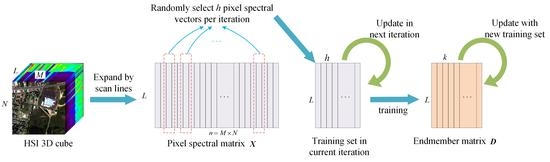
According to the principle of the aforementioned online dictionary learning, the steps of the proposed endmember extraction approach can be summarized as follows. Firstly, we select a random sequence of pixel spectral vectors from the observed HSI data, $X$, as the current training set. Next, for the training set in the current cycle, the abundances are found and the current endmember matrix is then updated. The proposed endmember extraction process is shown in Figure 1.

In this paper, we performed the online updating for the objective function with the $l_1$ norm data fitting term. Due to the non-smooth $l_1$ norm terms, solving the optimization problem of Equation (3) is somewhat challenging.

The optimization of Equation (3) is a robust sparse coding problem with respect to the optimization of the abundance coefficient $a_i$. When the endmember matrix $D$ is given, this robust sparse coding problem can be formulated as

$$a_i=\arg \underset{a_i\ge 0}{\min }{\Vert x_i-D{a}_i\Vert }_1^1+\lambda {\Vert a_i\Vert }_1,i=1,\dots ,n$$

(4)

Equation (4) represents an $l_1$ measured and $l_1$ regularized convex optimization. We solve the optimization problem of Equation (4) with an equivalent $l_1$ approximation robust sparse coding scheme [24].

When the abundance matrix is known, we can obtain the endmember matrix $D$ by minimizing the function as

$$g_t\left(D\right)=\frac{1}{t}{\displaystyle \sum _{\eta =1}^t{\Vert X^{\eta }-D{A}^{\eta }\Vert }_1^1+\lambda {\Vert A^{\eta }\Vert }_1}$$

(5)

where $t$ is the current iteration number, $X^{\eta }$ is the training set consisting of $h$ spectral vectors that are randomly obtained from the pixel spectral matrix $X$, and the corresponding abundance matrix $A^{\eta }$ is already known. Thus, the second $l_1$ norm term is constant here. Equation (5) is a standard $l_1$ regression problem, which lacks differentiability. Therefore, iterative reweighted least squares (IRLS) [25] are utilized to optimize the minimization problem of Equation (5).

The $j-\mathrm{th}$ column of $D$ is defined as $d_j$. Considering the independence of the estimation of each $d_j$, without loss of generality, the corresponding optimization function can be represented as

$$d_j=\arg \underset{D\left(j,:\right)}{\min }\frac{1}{h}{\displaystyle \sum _{i=1}^h\left|x_{ij}^t-d_j{a}_i^t\right|},$$

(6)

where $d_j\in {\mathbf{R}}^{1\times k}$, and $x_{ij}^t$ is the $j-\mathrm{th}$ element of the pixel spectral vector $x_i^t$ in the current training set $X^t$. According to the theory of IRLS, Equation (6) can be converted to the following two problems:

$$d_j=\arg \underset{D\left(j,:\right)}{\min }\frac{1}{h}{\displaystyle \sum _{i=1}^h{\omega }_{ij}^t{\left(x_{ij}^t-d_j{a}_i^t\right)}^2}$$

(7)

$${\omega }_{ij}^t=\frac{1}{\sqrt{{\left(x_{ij}^t-d_j{a}_i^t\right)}^2+\delta }}$$

(8)

where $\delta$ is a very small positive value. In this paper, $\delta$ is set to machine precision. Considering robust statistical characteristics, the weighted squared term in Equation (7) is a reasonable approximation of the $l_1$-norm term in Equation (6). Then, we should minimize a quadratic objective function shown in Equation (7) in each iteration. We can obtain the global optimum by taking the derivatives and setting them to zero. Thus, we can represent the objective function of the optimization problem in Equation (7) as

$$F\left(d_j\right)={\displaystyle \sum _{i=1}^h{\omega }_{ij}^t{\left(x_{ij}^t-d_j{a}_i^t\right)}^2}$$

(9)

To obtain the derivative of Equation (9), we have

$$\frac{\partial F\left(d_j\right)}{\partial d_j}={\displaystyle \sum _{i=1}^h{\omega }_{ij}^t{x}_{ij}^t{\left(a_i^t\right)}^{\mathrm{T}}}-d_j·{\displaystyle \sum _{i=1}^h{\omega }_{ij}^t{a}_i^t{\left(a_i^t\right)}^{\mathrm{T}}}$$

(10)

Then, we set Equation (10) to be zero, and obtain

$${\displaystyle \sum _{i=1}^h{\omega }_{ij}^t{x}_{ij}^t{\left(a_i^t\right)}^{\mathrm{T}}}=d_j·{\displaystyle \sum _{i=1}^h{\omega }_{ij}^t{a}_i^t{\left(a_i^t\right)}^{\mathrm{T}}}.$$

(11)

We cannot follow Equation (11) directly, since the optimized value of $d_j$ here is obtained only by the training set in the current iteration. Because a fixed small size of the new training set is used to update the dictionary at each iteration in the online scheme, we should take the statistical information of historical data (the previous $t-1$ training sets) into account. Therefore, we set

$$M_j^t=M_j^{t-1}+{\displaystyle \sum _{i=1}^h{\omega }_{ij}^t{a}_i^t{\left(a_i^t\right)}^{\mathrm{T}}}$$

(12)

$$C_j^t=C_j^{t-1}+{\displaystyle \sum _{i=1}^h{\omega }_{ij}^t{x}_{ij}^t{\left(a_i^t\right)}^{\mathrm{T}}}$$

(13)

$$M_j^1={\displaystyle \sum _{i=1}^h{\omega }_{ij}^1{a}_i^1{\left(a_i^1\right)}^{\mathrm{T}}}$$

(14)

$$C_j^1={\displaystyle \sum _{i=1}^h{\omega }_{ij}^1{x}_{ij}^1{\left(a_i^1\right)}^{\mathrm{T}}}$$

(15)

From Equations (12) and (13), we can find that the information for the current training set is stored in ${\displaystyle \sum _{i=1}^h{\omega }_{ij}^t{a}_i^t{\left(a_i^t\right)}^{\mathrm{T}}}$ and ${\displaystyle \sum _{i=1}^h{\omega }_{ij}^t{x}_{ij}^t{\left(a_i^t\right)}^{\mathrm{T}}}$.

Therefore, we can obtain $d_j$ in the following linear system:

$$C_j^t=d_j·M_j^t.$$

(16)

A conjugate gradient approach is used here to solve Equation (16), and $D^{t-1}$ in the previous iteration is used as the initialization in the current iteration, termed a warm start. Since $M_j^t$ is usually diagonally dominant, reasonable initialization is helpful for the rapid convergence of the conjugate gradient update.

With the aforementioned analysis, the proposed EEORDL flow can now be obtained. First, a set of pixel spectral vectors are randomly selected from the observed HSI data as the training set in the current iteration. Then, for each training set, we perform the robust sparse coding first, and then update the endmember matrix. The endmember matrix $D$ can be finally obtained with iterative convergence. Algorithm 1 shows the pseudo code for EEORDL.

Algorithm 1: Endmember extraction based on online dictionary learning (EEORDL)

Input: observed HSI $X\in {\mathbf{R}}^{L\times n}$, iterations $T\in \mathrm{N}$,    the number of the pixel spectral vectors used per iteration $h\in \mathrm{N}$

Output: endmember matrix $D\in {\mathbf{R}}^{L\times k}$

1 Preprocessing: Estimate the number of endmembers $k$ with HySime [26]

2 Initialization: Initialize the endmember matrix $D_0\in {\mathbf{R}}^{L\times k}$ with VCA;

3       Given $D_0$, initialize the abundance matrix $A_0\in {\mathbf{R}}^{k\times n}$ with nonnegative        least squares algorithm: $A_0=\arg {\min }_{A\ge 0}{\left|\right|X-D_0{A}_0\left|\right|}_F^2$

4   for $t=1$ to $T$ do

5   Draw randoml $X^t=\left[x_i^t,i=1,\dots ,h\right]$ from $X$

/* abundances update (robust sparse coding) */

6   for $i=1$ to $h$ do

7     $a_i^t=\arg \underset{a_i^t\ge 0}{\min }{\Vert x_i^t-D{a}_i^t\Vert }_1^1+\lambda {\Vert a_i^t\Vert }_1$

8   end for

/* endmembers update */

9   repeat

10     for $j=1$ to $k$ do

11       $M_j^t=M_j^{t-1}+{\displaystyle \sum _{i=1}^h{\omega }_{ij}^t{a}_i^t{\left(a_i^t\right)}^{\mathrm{T}}}$

12       $C_j^t=C_j^{t-1}+{\displaystyle \sum _{i=1}^h{\omega }_{ij}^t{x}_{ij}^t{\left(a_i^t\right)}^{\mathrm{T}}}$

13       solve linear system $C_j^t=d_j·M_j^t$

14       ${\omega }_{ij}^t=\frac{1}{\sqrt{{\left(x_{ij}^t-d_j{a}_i^t\right)}^2+\delta }},$

15      end for

16     until convergence

17   end for

18   return endmember matrix $D$

3. Experiments and Results

We used both synthetic data and real-world data in experiments to verify the effectiveness and competitiveness of the EEORDL proposed in this paper. The results were also compared with the current representative, effective hyperspectral endmember extraction algorithms, and the performance of each algorithm is comprehensively evaluated—both qualitatively and quantitatively. The experiments were implemented with MATLAB R2018a on a laptop equipped with eight Intel Core i7-7700HQ CPU and 16 GB RAM.

Five existing methods were used for comparison. Among them, VCA is a classical pure pixel-based approach and it is also the initialization method for the proposed EEORDL; PCOMMEND is based on the multiple convex region assumption; MVC-NMF and R-CoNMF are non-negative matrix factorization-based endmember generation algorithms; and EEODL is an online dictionary learning-based method.

3.1. Evaluation Indexes

Performance indexes used to evaluate the quality of the extracted endmembers include spectral angle distance (SAD) and spectral information divergence (SID).

SAD was used to measure the geometric feature difference between two spectral vectors, and can be represented as

$$\mathrm{SAD}={\cos }^{-1}\left(\frac{a^T\widehat{a}}{\Vert a\Vert ·\Vert \widehat{a}\Vert }\right)$$

(17)

where $a$ is the true endmember signature and $\widehat{a}$ is the estimated one.

The information theoretic index, SID, reflects the variability of the spectral vectors based on the probability of the difference of elements in two vectors, and can be expressed as

$$\mathrm{SID}=D\left(a|\widehat{a}\right)+D\left(\widehat{a}|a\right)$$

(18)

where

$$D\left(a|\widehat{a}\right)={\displaystyle \sum _j{p}_j\log \left(\frac{p_j}{{\widehat{p}}_j}\right)}$$

(19)

$$p_j=a_j/{\displaystyle {\sum }_j{a}_j}$$

(20)

Overall performance metrics for unmixing methods mainly include root mean square error (RMSE) and signal to reconstruction error (SRE) [27]. SRE considers the relation between the signal power and the error power, and can be calculated as

$$\mathrm{SRE}\left(\mathrm{dB}\right)=10{\log }_{10}\left(\frac{\mathrm{E}\left[{\Vert X\Vert }_2^2\right]}{\mathrm{E}\left[{\Vert \widehat{X}-X\Vert }_2^2\right]}\right)$$

(21)

3.2. Synthetic Data

The synthetic data discussed in this subsection are a representative dataset for hyperspectral unmixing [27]. The dataset was generated by nine spectral signatures, containing $100\times 100$ pixels. The abundance coefficient is piecewise smooth and spatial homogenous; thus it resembles that in real situations. Similar to the noise in real scenarios, correlated noise was used here. In the experiments, the noise was obtained by applying a low pass filter on independent and identically distributed (i.i.d) Gaussian noise, normalizing cut-off frequency at $5\pi /L$. The algorithms were performed at SNRs of 15 dB, 20 dB, 25 dB, 30 dB, and 35 dB, respectively.

To investigate the performance of each algorithm, after the endmember extraction of all the algorithms, the non-negative least squares algorithm was used to estimate the corresponding abundances to reconstruct the observed image. By calculating the corresponding RMSE and SRE values of different algorithms, the effects of their endmember extraction performance on the final spectral unmixing were compared.

Table 1. Quantitative assessment of different endmember extraction algorithms with synthetic data.

SNR (dB)	Index	VCA	PCOMMEND	MVCNMF	RCoNMF	EEODL	EEORDL
35	SAD(deg)	0.3638	1.153	0.2452	1.792	0.5196	0.2618
	SID	9.992 × 10−5	1.036 × 10−3	9.160 × 10−5	4.803 × 10−3	2.660 × 10−4	5.861 × 10−5
	RMSE	7.995 × 10−4	4.890 × 10−3	2.994 × 10−4	2.900 × 10−3	1.108 × 10−3	3.589 × 10−4
	SRE(dB)	24.04	17.54	27.76	17.60	22.19	27.13
30	SAD(deg)	0.7552	1.555	0.5469	2.281	0.5993	0.4396
	SID	5.623 × 10−4	3.083 × 10−3	3.174 × 10−4	7.843 × 10−3	2.674 × 10−4	1.315 × 10−4
	RMSE	2.204 × 10−3	1.691 × 10−2	1.102 × 10−3	5.123 × 10−3	2.822 × 10−3	1.087 × 10−3
	SRE(dB)	19.16	12.06	22.19	14.97	18.58	22.62
25	SAD(deg)	0.9223	1.694	1.026	2.916	1.1567	0.6113
	SID	8.529 × 10−4	3.413 × 10−3	1.200 × 10−3	1.160 × 10−2	1.119 × 10−3	2.615 × 10−4
	RMSE	5.362 × 10−3	1.817 × 10−2	2.912 × 10−3	8.702 × 10−3	1.030 × 10−2	3.085 × 10−3
	SRE(dB)	15.73	11.41	17.69	12.53	13.28	17.96
20	SAD(deg)	2.092	1.857	1.937	2.977	1.166	0.6810
	SID	4.534 × 10−3	4.285 × 10−3	4.812 × 10−3	1.180 × 10−2	1.072 × 10−3	2.989 × 10−4
	RMSE	1.382 × 10−2	2.356 × 10−2	8.034 × 10−3	1.724 × 10−2	1.061 × 10−2	7.457 × 10−3
	SRE(dB)	11.10	9.751	13.18	9.499	12.32	14.10
15	SAD(deg)	5.354	2.818	7.571	3.650	2.039	1.854
	SID	4.605 × 10−3	7.895 × 10−3	2.060 × 10−2	9.406 × 10−3	2.769 × 10−3	1.946 × 10−3
	RMSE	6.076 × 10−2	3.880 × 10−2	4.991 × 10−2	3.153 × 10−2	2.910 × 10−2	2.708 × 10−2
	SRE(dB)	5.178	7.111	6.212	6.908	8.360	8.834

reports the endmember extraction evaluation of different algorithms with the synthetic data. Most approaches achieve good results under a high level of SNR. When the level of SNR is gradually reduced, the performance of each algorithm deteriorates to varying degrees. Since the proposed EEORDL is initialized with VCA, the performance of the latter is also compared in Table 1. When SNR > 25 dB, MVCNMF achieves very good results, but the performance decreases rapidly when SNR is less than 20 dB. Since RCoNMF is somewhat sensitive to noise, its endmember extraction performance is rather poor under various SNR conditions. PCOMMEND has a relatively stable performance under different noise levels, and the performance is somewhat better than RCoNMF. EEODL achieves very good results, especially under low SNR conditions, exhibiting the advantages of dictionary learning and sparse representation theory applied to hyperspectral endmember extraction. Since the proposed EEORDL uses robust $l_1$ loss as the data fitting term in the objective function, it achieves better endmember extraction than EEODL. In a word, the proposed EEORDL achieves the best or comparable results under all SNR conditions, especially when SNR is low.

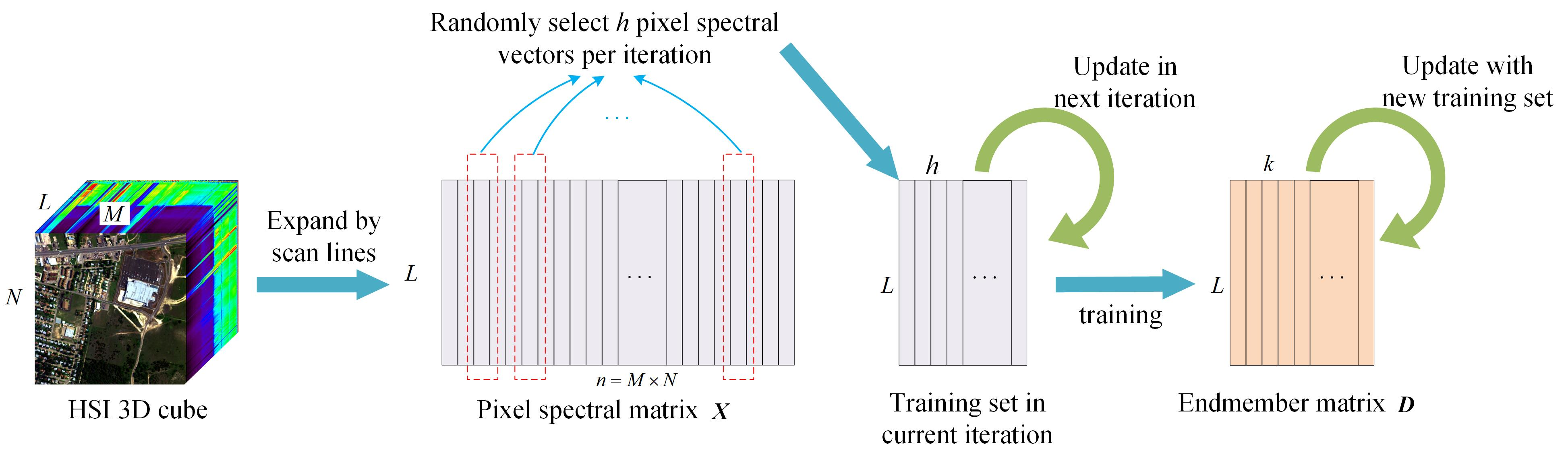
Figure 2 shows the endmember estimates obtained by different algorithms for SNR = 20 dB. It can be seen that the endmember signatures extracted by the proposed EEORDL have the highest degree of similarity to the ground truth spectral signatures, illustrating the qualitative accuracy of the endmember extraction of the proposed approach. With the other algorithms, it is difficult to ensure that all endmember spectral signatures are well matched with the ground truth spectra at the same time.

Table 2. The computational time of different endmember extraction algorithms with synthetic data.

	VCA	PCOMMEND	MVCNMF	RCoNMF	EEODL	EEORDL
Time/s	1.0	513.2	58.0	11.1	13.3	3.4

reports the computational time of different algorithms when SNR = 20 dB. It can be seen that the proposed EEORDL takes less running time than the other algorithms, except for VCA. We notice that EEORDL is significantly faster than EEODL, which indicates that the dictionary update in the proposed approach is more efficient.

3.3. Real-World Data

3.3.1. Jasper Ridge Dataset

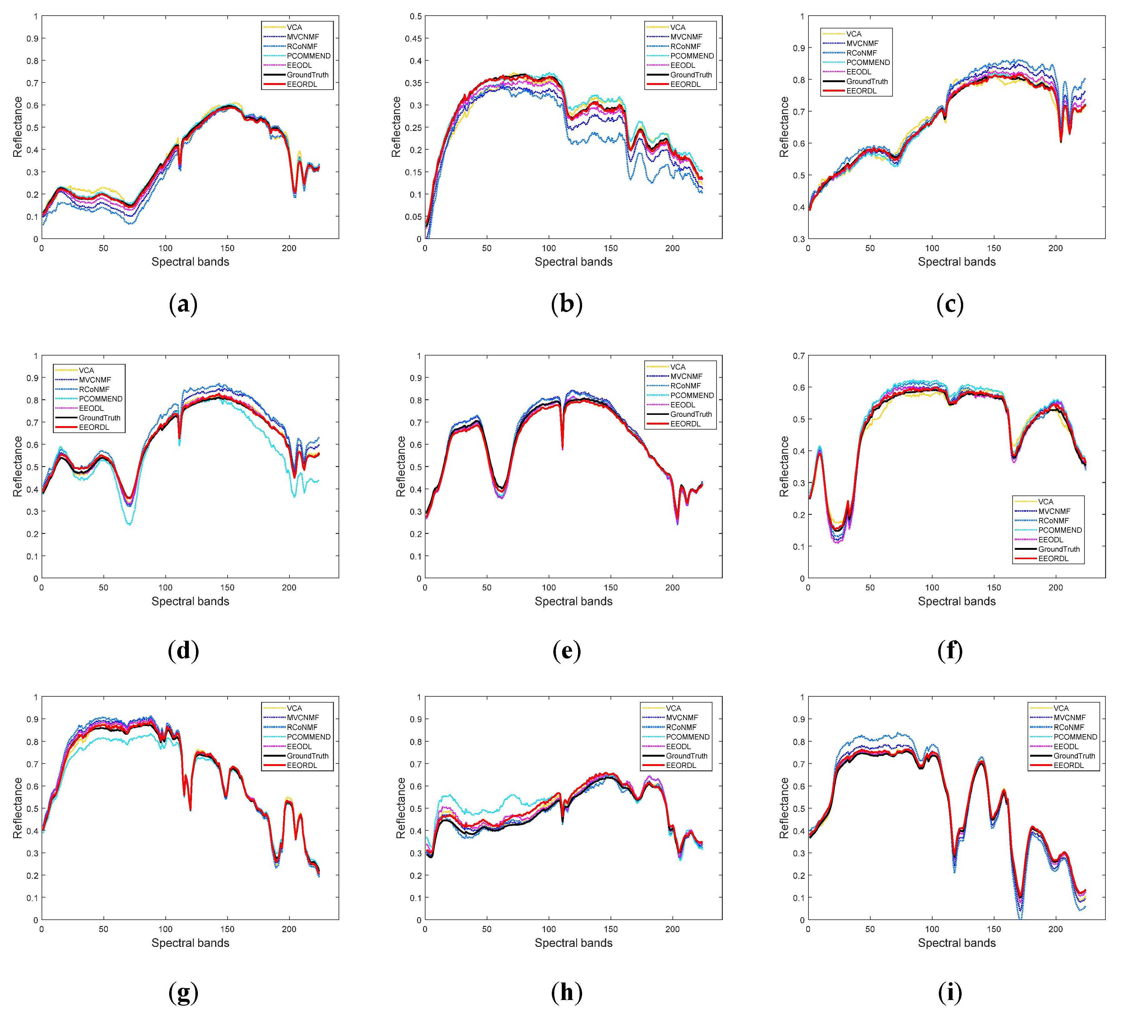
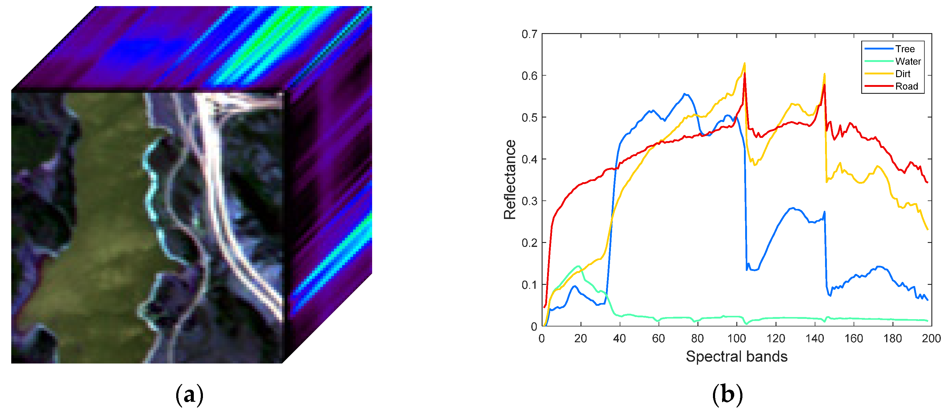
The popular Jasper Ridge dataset [28] was used as the real-world data in this subsection. The image includes 224 spectral bands between 0.4 and 2.5 $\mathsf{\mu }\mathrm{m}$, with a high spectral resolution of 10 nm. For the convenience of analysis, a sub-image of 100 $\times$ 100 pixels was selected here, as shown in Figure 3a. Water vapor absorption bands and blank bands (1–3, 108–112, 154–166, 220–224) were removed during data preprocessing, and 198 spectral bands were retained. Figure 3b shows four reference endmember spectra latent in the data, including trees, water, dirt and roads. In this dataset, the noise intensity varies with different bands.

The SAD values of different algorithms with the Jasper Ridge dataset are reported in

Table 3. SAD values of different endmember extraction algorithms with the Jasper Ridge dataset.

Endmember	VCA	PCOMMEND	MVCNMF	RCoNMF	EEODL	EEORDL
Tree	0.3228	0.1202	0.1705	0.2190	0.1897	0.1152
Water	0.2484	0.1889	0.9896	0.9460	0.2342	0.1105
Dirt	0.2263	0.1538	0.1567	0.1305	0.1601	0.1169
Road	0.2657	0.1120	0.1033	0.0546	0.0603	0.0502
Mean	0.2658	0.1437	0.3550	0.3375	0.1611	0.0982

, which illustrates that the proposed EEORDL achieves the best endmember extraction results for all four endmembers, quantitatively. To qualitatively confirm this conclusion, Figure 4 shows the endmember estimates obtained by different algorithms. We can see that the endmember signatures estimated by EEORDL have the highest degree of similarity to the references. In contrast, with the other methods it is difficult to ensure that all four endmember estimates can be well matched with the reference spectra at the same time.

3.3.2. Urban Dataset

The urban dataset is widely used in the hyperspectral unmixing field [28], consisting of 307 $\times$ 307 pixels. Each pixel in the image includes 210 spectral bands ranging from 0.4 $\mathsf{\mu }\mathrm{m}$ to 2.5 $\mathsf{\mu }\mathrm{m}$, resulting in a nominal spectral resolution of 10 nm. Figure 5a shows the 3D cube form of the dataset. Considering dense water vapor and atmospheric effects, the bands 1–4, 76, 87, 101–111, 136–153 and 198–210 were removed before endmember extraction, and 162 spectral bands were retained. Four reference endmember signatures that are latent in the data are shown in Figure 5b, including asphalt, grass, trees and roofs. As presented in [29], some bands in the data are also corrupted by sparse noise.

Table 4. SAD values of different endmember extraction algorithms with the Urban dataset.

Endmember	VCA	PCOMMEND	MVCNMF	RCoNMF	EEODL	EEORDL
Asphalt	0.1331	0.1055	0.1840	0.2450	0.1770	0.0999
Grass	0.3982	0.4568	0.5130	0.6206	0.3893	0.1258
Tree	0.0848	0.0541	0.1594	0.3587	0.1799	0.0530
Roof	0.1676	0.1135	0.1142	0.1640	0.2795	0.1075
Mean	0.1959	0.1825	0.2427	0.3347	0.2564	0.0966

reports the SAD values between the endmember estimates and their corresponding references from different algorithms with the Urban dataset. It can be seen that the proposed EEORDL outperforms the other algorithms and obtains the best endmember estimation results, quantitatively. To evaluate the endmember extraction performance of EEORDL qualitatively, Figure 6 shows the endmembers extracted by different approaches. The endmember signatures extracted by the proposed method obtain a good match with the references. In contrast, with the compared methods it is difficult to guarantee the similarity between the estimates and the references, especially for the endmember ‘grass’, as shown in Figure 6b.

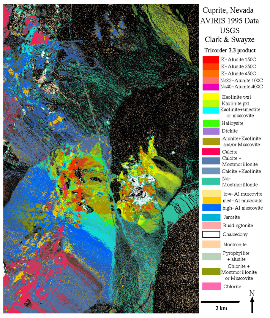
3.3.3. Cuprite Dataset

The well-known Cuprite dataset (http://aviris.jpl.nasa.gov/html/aviris.freedata.html) was used as the real-world data in this subsection. The image scene was collected by AVIRIS, including 224 spectral bands between 0.4 and 2.5 $\mathsf{\mu }\mathrm{m}$, with a nominal spectral resolution of 10 nm. For the convenience of analysis, a sub-image of 250 $\times$ 330 pixels was selected here, as shown in Figure 7. Water vapor absorption bands and low SNR bands (1–2, 105–115, 150–170, 223–224) were eliminated during data preprocessing, and 188 spectral bands were retained. The mineral signatures contained in the Cuprite dataset were released in the USGS spectral library under the name splib06 (http://speclab.cr.usgs.gov/spectral.lib06), in September 2007. Thus, the endmember extraction performance of the proposed EEORDL can be verified by using the corresponding USGS library spectral signatures. Since a large number of mineral alterations and spectral variabilities are presented in the Cuprite dataset, there is no official agreement on the number of material spectral signatures. According to the analysis in [21,30], we set the number of endmembers in the experiment as $p=12$.

To investigate the performance of the proposed EEORDL after the endmember extraction, the non-negative least squares algorithm was used to estimate the corresponding abundances. We used the MATLAB function lsqnonneg to perform the abundance estimation in this experiment. Considering that the true abundance maps are unknown, the results of the abundance estimation were only evaluated qualitatively by using a material map produced by Tricorder 3.3 software (http://speclab.cr.usgs.gov/cuprite95.tgif.2.2um_map.gif) as a reference, as shown in Figure 8.

Table 5. SAD values of different endmember extraction algorithms with the Cuprite dataset.

Endmember	VCA	PCOMMEND	MVCNMF	RCoNMF	EEODL	EEORDL
Alunite GDS84 Na03	0.1069	0.1331	0.1070	0.0889	0.1158	0.0864
Andradite	0.0782	0.0726	0.1018	0.2864	0.0791	0.0718
Buddingtonite GDS85 D-206	0.2019	0.1661	0.2189	0.3351	0.2373	0.1656
Dumortierite	0.1375	0.0894	0.1804	0.1517	0.0881	0.0880
Kaolinite KGa-2 (pxyl)	0.2642	0.1118	0.3588	0.1072	0.2560	0.1121
Kaolin/Smect KLF508 85%K	0.0759	0.0893	0.0942	0.1471	0.1309	0.0906
Muscovite IL107	0.1485	0.1217	0.1637	0.0705	0.1260	0.1216
Montmorillonite+Illi CM37	0.1035	0.0605	0.1252	0.0727	0.1011	0.0600
Nontronite SWa-1.a	0.1072	0.1163	0.1776	0.1079	0.1551	0.1164
Kaolin/Smect H89-FR-5 30K	0.0817	0.0820	0.0987	0.0947	0.1574	0.0795
Sphene	0.0658	0.0543	0.0685	0.2036	0.0626	0.0539
Chalcedony CU91-6A	0.0666	0.0720	0.0737	0.4807	0.0639	0.0748
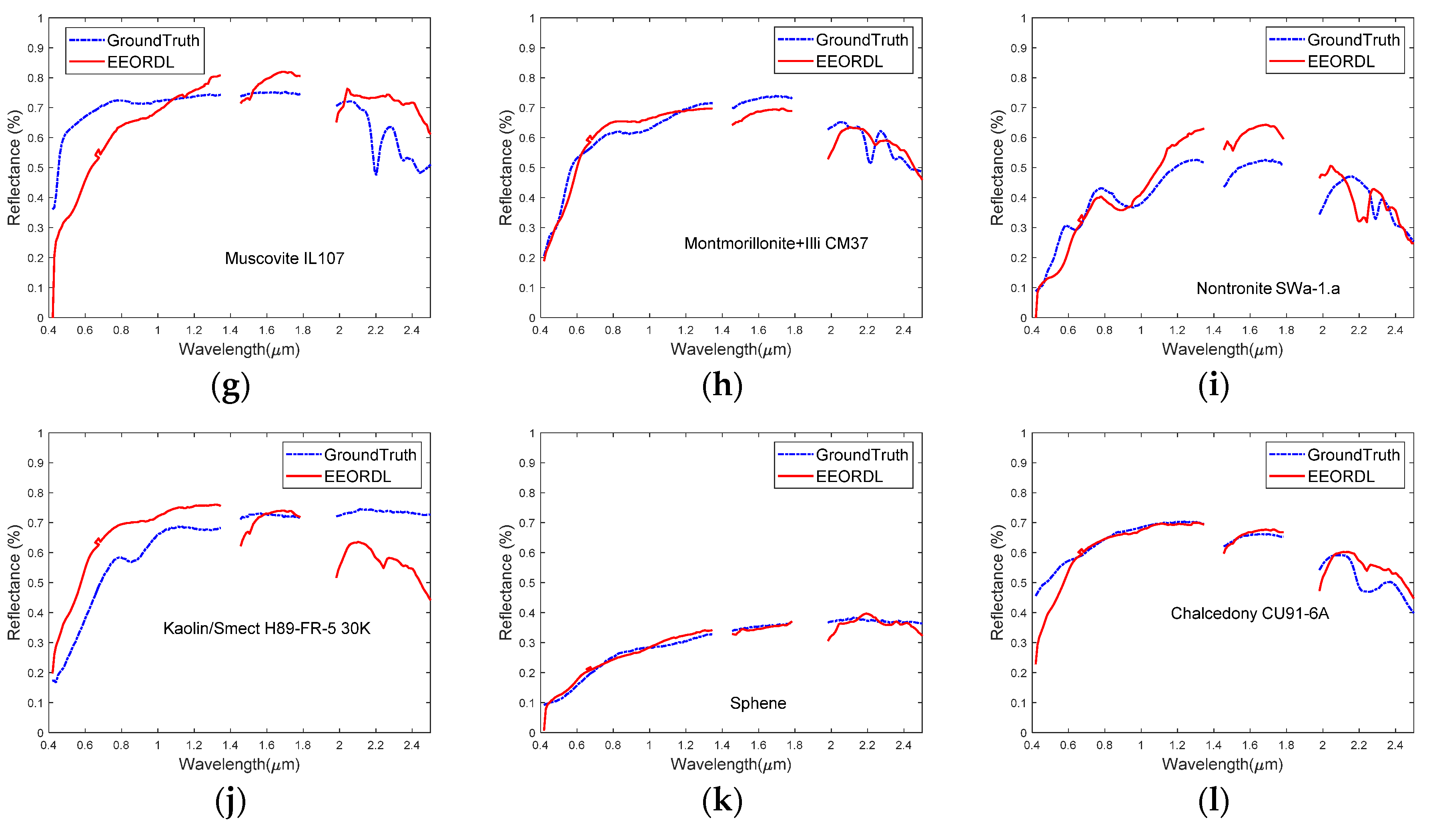
Mean	0.1198	0.0974	0.1474	0.1789	0.1311	0.0934

reports the SAD values between the endmember estimates and their corresponding USGS library spectral signatures of different algorithms with the Cuprite dataset. It can be concluded that the proposed EEORDL achieved the best endmember extraction results for over half of all 12 endmembers. In addition, EEORDL obtained the best mean SAD results, which demonstrates the effectiveness and competitiveness of the proposed approach.

Figure 9 shows the endmember estimates obtained by the proposed EEORDL along with their corresponding USGS library spectral signatures. Considering the reference signatures from the USGS library acquired without atmospheric interferers and in ideal conditions, the results shown in Figure 9 illustrate that the extracted endmembers generally achieve a good match with the corresponding references.

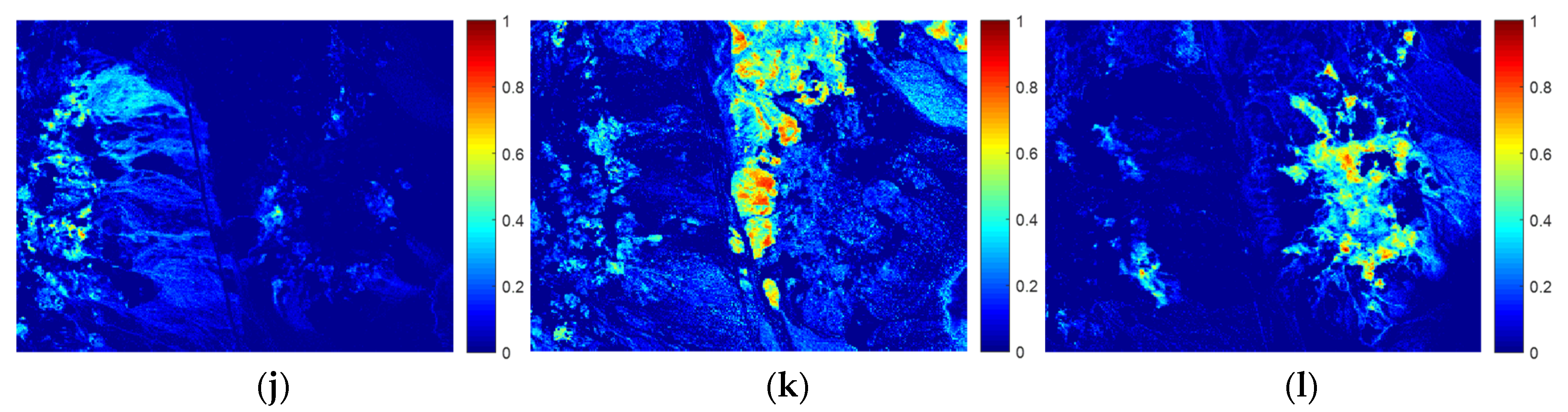
Figure 10 shows the corresponding estimated abundance maps obtained by the non-negative least-squares algorithm. Moreover, it can be observed in Figure 10 that the estimated abundance maps are piecewise smooth and have high spatial consistency, further demonstrating that the proposed EEORDL can efficiently complete the endmember extraction task in spectral unmixing.

4. Conclusions

In this paper, an endmember extraction algorithm based on online robust dictionary learning, termed EEORDL, was proposed to solve the problem of endmember estimation in a noisy environment. Unlike the current dictionary learning-based endmember extraction methods, in EEORDL, a more robust $l_1$ norm is used as the data fitting term during the dictionary update to improve the performance of the endmember extraction. Compared with the state-of-the-art endmember extraction approaches, the proposed EEORDL achieves better performance, especially under the conditions of low SNR. Because of these aforementioned properties, the proposed algorithm may have a positive impact on hyperspectral subpixel target detection.

References

- Xu, X.; Shi, Z.; Pan, B. ℓ0-based sparse hyperspectral unmixing using spectral information and a multi-objectives formulation. ISPRS J. Photogramm. Remote Sens. 2018, 141, 46–58. [Google Scholar] [CrossRef]
- Zou, Z.; Shi, Z. Hierarchical Suppression Method for Hyperspectral Target Detection. IEEE Trans. Geosci. Remote Sens. 2015, 54, 330–342. [Google Scholar] [CrossRef]
- Pan, B.; Shi, Z.; Xu, X.; Shi, T.; Zhang, N.; Zhu, X. CoinNet: Copy Initialization Network for Multispectral Imagery Semantic Segmentation. IEEE Geosci. Remote Sens. Lett. 2018, 16, 816–820. [Google Scholar] [CrossRef]
- Liu, S.C.; Bruzzone, L.; Bovolo, F.; Du, P.J. Unsupervised Multitemporal Spectral Unmixing for Detecting Multiple Changes in Hyperspectral Images. IEEE Trans. Geosci. Remote Sens. 2016, 54, 2733–2748. [Google Scholar] [CrossRef]
- Bioucas-Dias, J.M.; Plaza, A.; Dobigeon, N.; Parente, M.; Du, Q.; Gader, P.; Chanussot, J. Hyperspectral Unmixing Overview: Geometrical, Statistical, and Sparse Regression-Based Approaches. IEEE J. Sel. Top. Appl. Earth Obs. Remote Sens. 2012, 5, 354–379. [Google Scholar] [CrossRef] [Green Version]
- Ma, W.K.; Bioucas-Dias, J.M.; Chan, T.H.; Gillis, N.; Chi, C.Y. A Signal Processing Perspective on Hyperspectral Unmixing: Insights from Remote Sensing. IEEE Signal Process. Mag. 2014, 31, 67–81. [Google Scholar] [CrossRef]
- Feng, R.; Wang, L.; Zhong, Y. Least Angle Regression-Based Constrained Sparse Unmixing of Hyperspectral Remote Sensing Imagery. Remote Sens. 2018, 10, 1546. [Google Scholar] [CrossRef]
- Iordache, M.D.; Bioucas-Dias, J.M.; Plaza, A. Sparse Unmixing of Hyperspectral Data. IEEE Trans. Geosci. Remote Sens. 2011, 49, 2014–2039. [Google Scholar] [CrossRef] [Green Version]
- Chen, S.; Le, W. Linear Spatial Spectral Mixture Model. IEEE Trans. Geosci. Remote Sens. 2016, 54, 3599–3611. [Google Scholar] [CrossRef]
- Chang, C.I.; Plaza, A. A Fast Iterative Algorithm for Implementation of Pixel Purity Index. IEEE Geosci. Remote Sens. Lett. 2006, 3, 63–67. [Google Scholar] [CrossRef]
- Nascimento, J.M.P.; Dias, J.M.B. Vertex component analysis: A Fast algorithm to unmix hyperspectral data. IEEE Trans. Geosci. Remote Sens. 2005, 43, 898–910. [Google Scholar] [CrossRef]
- Winter, M.E. N-FINDR: An Algorithm for Fast Autonomous Spectral Endmember Determination in Hyperspectral Data. Proc. SPIE 1999, 3753, 266–275. [Google Scholar] [CrossRef]
- Yao, S.; Zeng, W.; Wang, N.; Chen, L. Validating the performance of one-time decomposition for fMRI analysis using ICA with automatic target generation process. Magn. Reson. Imaging 2013, 31, 970–975. [Google Scholar] [CrossRef] [PubMed]
- Wu, C.C.; Lo, C.S.; Chang, C.L. Improved Process for Use of a Simplex Growing Algorithm for Endmember Extraction. IEEE Geosci. Remote Sens. Lett. 2009, 6, 523–527. [Google Scholar] [CrossRef]
- Li, J.; Agathos, A.; Zaharie, D.; Bioucas-Dias, J.M.; Li, X. Minimum Volume Simplex Analysis: A Fast Algorithm for Linear Hyperspectral Unmixing. IEEE Trans. Geosci. Remote Sens. 2015, 53, 5067–5082. [Google Scholar] [CrossRef]
- Miao, L.; Qi, H. Endmember Extraction from Highly Mixed Data Using Minimum Volume Constrained Nonnegative Matrix Factorization. IEEE Trans. Geosci. Remote Sens. 2007, 45, 765–777. [Google Scholar] [CrossRef]
- Li, J.; Bioucasdias, J.M.; Plaza, A.; Lin, L. Robust Collaborative Nonnegative Matrix Factorization for Hyperspectral Unmixing (R-CoNMF). IEEE Trans. Geosci. Remote Sens. 2016, 54, 6076–6090. [Google Scholar] [CrossRef]
- Zare, A.; Gader, P.; Bchir, O.; Frigui, H. Piecewise Convex Multiple-Model Endmember Detection and Spectral Unmixing. IEEE Trans. Geosci. Remote Sens. 2013, 51, 2853–2862. [Google Scholar] [CrossRef]
- Liu, Y.; Guo, Y.; Li, F.; Xin, L.; Huang, P. Sparse Dictionary Learning for Blind Hyperspectral Unmixing. IEEE Geosci. Remote Sens. Lett. 2019, 16, 578–582. [Google Scholar] [CrossRef]
- Song, X.; Wu, L.; Hao, H. Blind hyperspectral sparse unmixing based on online dictionary learning. In Proceedings of the Image and Signal Processing for Remote Sensing XXIV, Berlin, Germany, 10–13 September 2018; p. 107890. [Google Scholar] [CrossRef]
- Qu, Y.; Qi, H. uDAS: An Untied Denoising Autoencoder With Sparsity for Spectral Unmixing. IEEE Trans. Geosci. Remote Sens. 2019, 57, 1698–1712. [Google Scholar] [CrossRef]
- Andrew, W.; John, W.; Arvind, G.; Zihan, Z.; Hossein, M.; Yi, M. Toward a practical face recognition system: Robust alignment and illumination by sparse representation. IEEE Trans. Pattern Anal. Mach. Intell. 2012, 34, 372. [Google Scholar] [CrossRef]
- Lu, C.; Shi, J.; Jia, J. Online Robust Dictionary Learning. In Proceedings of the IEEE Conference on Computer Vision and Pattern Recognition, Portland, OR, USA, 23–28 June 2013. [Google Scholar] [CrossRef]
- Zhao, C.; Wang, X.; Cham, W.K. Background Subtraction via Robust Dictionary Learning. EURASIP J. Image Video Process. 2011, 2011, 1–12. [Google Scholar] [CrossRef] [Green Version]
- Bissantz, N.; Dümbgen, L.; Munk, A.; Stratmann, B. Convergence analysis of generalized iteratively reweighted least squares algorithms on convex function spaces. Tech. Rep. 2008, 19, 1828–1845. [Google Scholar] [CrossRef]
- Bioucas-Dias, J.M.; Nascimento, J.M.P. Hyperspectral subspace identification. IEEE Trans. Geosci. Remote Sens. 2008, 46, 2435–2445. [Google Scholar] [CrossRef]
- Iordache, M.-D.; Bioucas-Dias, J.M.; Plaza, A. Total variation spatial regularization for sparse hyperspectral unmixing. IEEE Trans. Geosci. Remote Sens. 2012, 50, 4484–4502. [Google Scholar] [CrossRef]
- Wang, Y.; Pan, C.; Xiang, S.; Zhu, F. Robust Hyperspectral Unmixing with Correntropy-Based Metric. IEEE Trans. Image Process. 2015, 24, 4027–4040. [Google Scholar] [CrossRef] [PubMed]
- He, W.; Zhang, H.; Zhang, L. Sparsity-Regularized Robust Non-Negative Matrix Factorization for Hyperspectral Unmixing. IEEE J. Sel. Top. Appl. Earth Obs. Remote Sens. 2016, 9, 4267–4279. [Google Scholar] [CrossRef]
- Wang, X.; Zhong, Y.; Zhang, L.; Xu, Y. Spatial Group Sparsity Regularized Nonnegative Matrix Factorization for Hyperspectral Unmixing. IEEE Trans. Geosci. Remote Sens. 2017, 55, 6287–6304. [Google Scholar] [CrossRef]
Figure 1.
The process of the proposed endmember extraction approach based on online robust dictionary learning (EEORDL). HSI: hyperspectral image. M is the number of samples in a single scan, N is the scan number in the image, L is the band number, h is the number of pixel spectral vectors used per iteration, and k is the number of endmembers.
Figure 2.
The endmember estimates obtained by different algorithms for SNR = 20 dB: (a) Actinolite HS116.3B; (b) Dry_Long_Grass; (c) Richterite; (d) Actinolite NMNHR16485; (e) Anthophyllite; (f) Lazurite; (g) Alunite; (h) Clinochlore; (i) Carnallite.
Figure 3.
Jasper Ridge hyperspectral dataset: (a) 3D cube form of the experiment area; (b) Reference spectral signatures.
Figure 4.
The endmember estimates obtained by different algorithms: (a) trees; (b) water; (c) dirt; (d) roads.
Figure 5.
Urban hyperspectral dataset: (a) 3D cube form of the experiment area; (b) Reference spectral signatures.
Figure 6.
The endmember estimates obtained by different algorithms: (a) Asphalt; (b) Grass; (c) Trees; (d) Roofs.
Figure 7.
3D cube form of the experiment area in the Cuprite hyperspectral dataset.
Figure 8.
Material map of the Cuprite dataset obtained by Tricorder 3.3 software.
Figure 9.
The extracted endmembers and their corresponding USGS library spectral signatures with the Cuprite data: (a) Alunite GDS84 Na03; (b) Andradite; (c) Buddingtonite GDS85 D-206; (d) Dumortierite; (e) Kaolinite KGa-2 (pxyl); (f) Kaolin/Smect KLF508 85%K; (g) Muscovite IL107; (h) Montmorillonite+Illi CM37; (i) Nontronite SWa-1.a; (j) Kaolin/Smect H89-FR-5 30K; (k) Sphene; (l) Chalcedony CU91-6A.
Figure 10.
The estimated abundance maps of the Cuprite data: (a) Alunite GDS84 Na03; (b) Andradite; (c) Buddingtonite GDS85 D-206; (d) Dumortierite; (e) Kaolinite KGa-2 (pxyl); (f) Kaolin/Smect KLF508 85%K; (g) Muscovite IL107; (h) Montmorillonite+Illi CM37; (i) Nontronite SWa-1.a; (j) Kaolin/Smect H89-FR-5 30K; (k) Sphene; (l) Chalcedony CU91-6A.