LiDAR DEM Smoothing and the Preservation of Drainage Features


Department of Geography, Environment & Geomatics, The University of Guelph, 50 Stone Rd. E, Guelph, ON N1G 2W1, Canada
*
Author to whom correspondence should be addressed.
Remote Sens. 2019, 11(16), 1926; https://0-doi-org.brum.beds.ac.uk/10.3390/rs11161926
Submission received: 21 July 2019
/
Revised: 7 August 2019
/
Accepted: 14 August 2019
/
Published: 17 August 2019
(This article belongs to the Special Issue Future Trends and Applications for Airborne Laser Scanning)
Abstract
:Fine-resolution Light Detection and Ranging (LiDAR) data often exhibit excessive surface roughness that can hinder the characterization of topographic shape and the modeling of near-surface flow processes. Digital elevation model (DEM) smoothing methods, commonly low-pass filters, are sometimes applied to LiDAR data to subdue the roughness. These techniques can negatively impact the representation of topographic features, most notably drainage features, such as headwater streams. This paper presents the feature-preserving DEM smoothing (FPDEMS) method, which modifies surface normals to smooth the topographic surface in a similar manner to approaches that were originally designed for de-noising three-dimensional (3D) meshes. The FPDEMS method has been optimized for application with raster DEM data. The method was compared with several low-pass filters while using a 0.5-m resolution LiDAR DEM of an agricultural area in southwestern Ontario, Canada. The findings demonstrated that the technique was better at removing roughness, when compared with mean, median, and Gaussian filters, while also preserving sharp breaks-in-slope and retaining the topographic complexity at broader scales. Optimal smoothing occurred with kernel sizes of 11–21 grid cells, threshold angles of 10°–20°, and 3–15 elevation-update iterations. These parameter settings allowed for the effective reduction in roughness and DEM noise and the retention of terrace scarps, channel banks, gullies, and headwater streams.
Keywords:
DEM; LiDAR; data smoothing; denoise; roughness; micro-topography; hydrology; geomorphometry; streams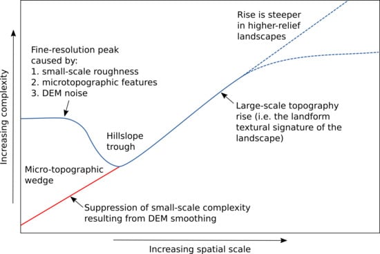
1. Introduction
Modern terrain mapping techniques that are based on Light Detection and Ranging (LiDAR) have allowed for accurate fine-resolution digital elevation model (DEM) production [1,2,3], with the ability to represent small-scale topographic variation [4]. At small spatial scales (<10 m), topographic surfaces are highly complex, owing to the prevalence of un-autocorrelated topographic variation, which contributes to the rough appearance of many LiDAR DEMs [5,6,7,8]. Small-scale surface roughness adds complexity to a DEM and it is often undesirable because of its impact on the characterization of larger-scale topography and because it confounds the measurement of geomorphometric indices, e.g., slope, aspect, curvature, and flow directions [9,10,11,12]. Surface roughness is a natural component of Earth’s topography, and therefore its presence in fine-resolution DEMs is expected. However, surface roughness is often removed from DEMs using various de-noising or smoothing techniques [4,9,13,14,15], most commonly including data reduction (e.g., grid resampling [16] and generalization [14,17,18,19]) and low-pass filters.
Low-pass filters are frequently applied to smooth DEMs to remove error and lessen roughness [9,20,21]. These filters suppress the short-scale signal corresponding to error/roughness, reduce local variation, and preserve the longer-range signal representing spatially autocorrelated information. However, low-pass filters have the tendency to blur edges, or breaks-in-slope [22]. Furthermore, most existing smoothing methods assume that the salient topographic features that are contained within a DEM exist at larger spatial scales than the unwanted variability. However, in fine-resolution LiDAR DEMs, the topographic expression of salient micro-topographic drainage features may also occupy scales that overlap with surface roughness. Many current approaches to filtering-based DEM smoothing are unable to explicitly preserve these salient micro-topographic drainage features. Many hydrological applications benefit from DEM representation of small drainage features, such as rills, ditches, gullies, and headwater channels, which exist at the same spatial scales as surface roughness [23,24]. Small drainage features often control modelled surface drainage patterns. Very often, it is the ability of LiDAR DEMs to represent these small-scale drainage features that provides the justification for the acquisition of these data in projects. Thus, it is counter-productive to smooth fine-resolution DEMs if the outcome is the removal of salient topographic information.
Edge-preserving low-pass filters aim to retain the sharpness of edge definition while smoothing the unstructured short-scale variation [25,26,27] and these techniques may be useful for preserving drainage features in LiDAR data. Although this family of filters has mainly been developed for application with digital imagery [26,27] and to de-noise three-dimensional (3D) mesh models [28,29,30,31,32], they have been applied previously to the smoothing of DEM data [13]. Stevenson et al. [13] used the Sun et al. [31] method to demonstrate that feature-preserving DEM de-noising was possible, at least for the coarse-resolution interferometric DEMs to which it was applied in that study. However, the Sun et al. [31] algorithm was not originally intended for data sets as large as typical LiDAR DEMs. Rather, the algorithm was designed to de-noise point cloud datasets of 3D object models, to which triangulated meshes are fit. When applied to raster data sets, Sun et al.’s [31] MDenoise program (i.e., the back-end of GRASS GIS’s r.denoise tool) proceeds by fitting a triangular irregular network (TIN) to each grid cell. This triangulation-based, iterative approach to smoothing is a highly inefficient workflow when it is applied to large raster DEMs. These computational factors can limit the practical usefulness of Sun et al.’s [31] method for application with LiDAR DEMs.
This study aims to explore the potential for feature-preserving smoothing for the removal of roughness in fine-resolution LiDAR DEMs in a way that can preserve small drainage features. To achieve this goal, we introduce a novel feature-preserving DEM smoothing (FPDEMS) method that has been specifically designed to work with the raster LiDAR data sets. The method is then compared with several common low-pass filters while using a 0.5-m resolution LiDAR DEM of an agricultural area in southwestern Ontario, Canada.
2. Materials and Methods
2.1. Feature-Preserving DEM Smoothing (FPDEMS)
The Feature Preserving DEM Smoothing (FPDEMS) algorithm was specifically designed to smooth raster DEMs, following the approach that is commonly used for 3D mesh model smoothing. Under the assumption that surface normals represent local surface geometry better than vertex position values, many mesh smoothing methods first smooth the normal vector field and then use this field to reconstruct the smoothed surface’s vertices [30,31,32]. Thus, these mesh-based techniques have three general steps: (1) calculate the normal vector field from the input surface, (2) smooth the normal vector field, and (3) use the smoothed normals to update the original vertex positions.
A surface normal is a 3D vector that is perpendicular to the tangent plane at a point of measurement. If the tangent plane to a point (x, y, z) on the surface is defined as,
the three components of the normal (n) are:
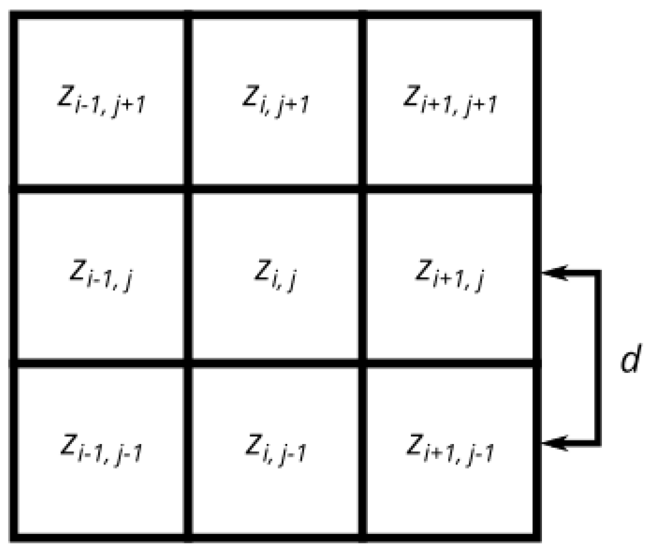
Mesh-based smoothing methods derive n for each face in the 3D model. These faces usually correspond to the triangular facets of a triangulation fit to the model vertices. Triangulation is a suitable way of inferring structure from 3D point clouds. However, triangulation is redundant for the elevations of a DEM, because the raster data structure itself permits the rapid and efficient querying of neighboring elevation values and the characterization of surface geometry [33]. Stevenson et al. [13] applied an implementation of Sun et al.’s [31] mesh smoothing method (available in GRASS GIS as the r.denoise tool) to de-speckle interferometric DEM data. While r.denoise works with either point clouds or raster data, it does appear to perform a triangulation on both data types. Therefore, surface normals are calculated for the eight triangular facets connecting each grid cell elevation to its neighbors. Triangulation of rasters is both computationally expensive and requires substantially more memory resources than necessary. The FPDEMS method, by comparison, calculates a single normal for each grid cell based on the 3rd order finite-difference surface-fitting scheme [33] that is commonly used in geomorphometric analysis to estimate slope gradient and aspect. One can derive the rates of change in elevation in the x and y directions from the eight outer elevations in the 3 × 3 window surrounding each grid cell in the DEM (Figure 1), using:
The normal components can then be derived from:
where is the magnitude of n, calculated in the following way:
Equations (5)–(8) provide formulations for directly deriving unit normals (i.e., vector magnitude = 1.0) from eight neighboring elevations. Unit normals are the canonical form of representing these data. If instead we choose not to normalize n, c = 1.0 and there is no need to store all three components of the normal vector field. This reduces the memory requirements of the normals by one-third and also reduces the number of calculations that are involved in smoothing of the field.
Another advantage of directly utilizing the inherent structure of a raster lies in the ability to use convolution filtering to smooth the normal vector field. Most of the mesh smoothing methods achieve broad-scale smoothing by applying multiple iterations of localized smoothing of the normals of adjacent triangular facets [28,29,30,31,32]. The FPDEMS method, by comparison, achieves broad-scale smoothing of the normal vector field by applying a filtering operation with kernel sizes of a user-specified width; larger kernels result in more aggressive DEM smoothing. Any low-pass filter operation could be used to smooth the normal vector field. The FPDEMS method uses the same feature-preserving low-pass scheme that was proposed by Sun et al. [31]. The filter kernel weights are larger for neighboring cells with normals that are well aligned with the kernel center cell normal, and the weights decrease as the angle between normals increases. The smoothed normal (n’i) for cell i is calculated as:
where N is the number of grid cells in the kernel and wj is the weight assigned to neighboring cells j. wj is computed while using the following conditional case:
The upper condition in Equation (10) occurs when the angle between the center-cell normal and the neighboring normal, is smaller than a user-specified threshold (θt). Neighbors with normal differences that are larger than θt are assigned a weight of zero, which effectively excludes them from the calculation of the cell i smoothed normal. This ensures that neighboring sites on different terrain facets, and thus separated by a break-in-slope, do not contribute to the smoothing operation.
After the normal vector field has been smoothed, elevations are iteratively updated while using the smoothed normals. An updated elevation for cell i is calculated based on the smoothed tangent planes of i’s eight neighbors (i.e., substituting n’j in Equation (1) and solving for zi at (xi, yi)), while using the same weighting scheme that is described in Equation (10). Again, neighbors with normal differences that are greater than the threshold angle are excluded (wj = 0). This elevation updating process continues for a user-specified number of iterations.
FPDEMS was implemented as the FeaturePreservingSmoothing tool within the open-source geospatial analysis platform WhiteboxTools [34]. The source code of the tool, developed using the Rust programming language, is available on the WhiteboxTools GitHub repository. Estimation of surface normals and the smoothing of the normal field are both parallelized in the FeaturePreservingSmoothing tool for improved computational efficiency. The iterative elevation updating step was the only portion of the workflow that was not parallelized. The user must specify the three main tool parameters, including the smoothing filter kernel size, the threshold normal difference angle (specified in degrees), and the number of elevation-update iterations. The user may also optionally restrict the elevation modifications to a maximum value. Elevation updates that are larger than this value are left unmodified.
2.2. Study Site and Data
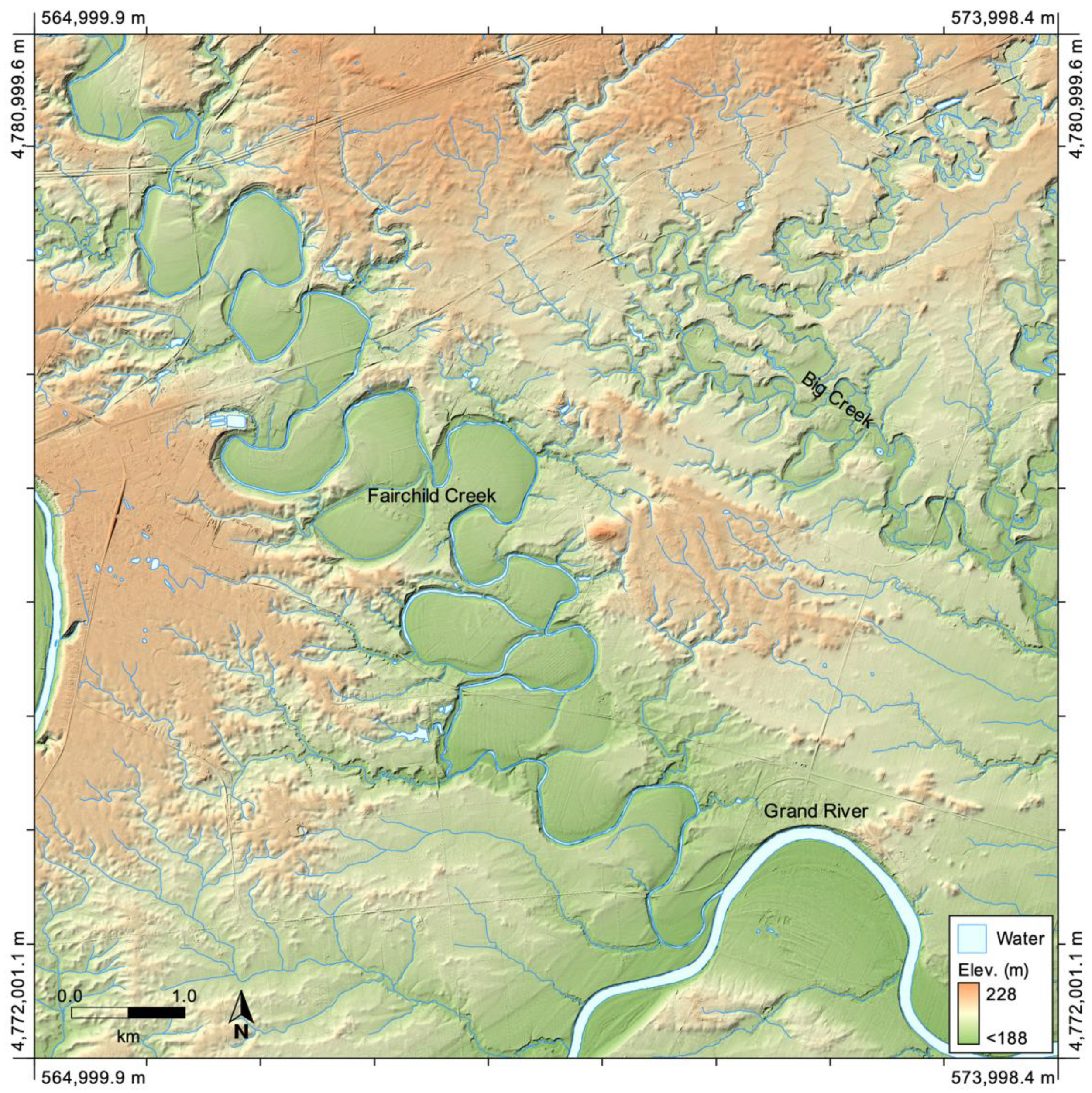
The FPDEMS smoothing algorithm was applied to a 324,000,000-grid cell (1.3 GB), 0.5-m resolution LiDAR DEM. The DEM covers an 81 km2 area east of Brantford Ontario, Canada (Figure 2). The study site is located between latitude and longitude ranges of 43°5′50″N to 43°10′44″N and 80°5′22″W to 80°12′5″W, respectively, and it overlaps with portions of the Big Creek and Fairchild Creek sub-basins, which are tributaries of the Grand River. Headwater streams tend to be deeply incised within the area. The large incised meanders of each of the major rivers exhibit broad floodplains that are bordered by steep paired terrace scarps, which is most evident in the case of the lower portion of Fairchild Creek. This creek cuts a prominent northwest-southeast diagonal through the study site. The steep terrace scarps that are associated with the streams provide significant local relief, although the overall relief of the study site is only 40 m. The physiography of the site largely consists of dissected sand plains and clay plains [35]. The majority of the study site is agricultural and there are some smaller forested areas that are scattered throughout. There are also small urbanized areas within the site, which are particularly associated with the outlying portions of Brantford, located towards the west.
The DEM was interpolated with a triangulation scheme from last- and only-returns of the source LiDAR point cloud. A private contractor that was commissioned by the Ontario Ministry of Agriculture, Food, and Rural Affairs (OMAFRA) and the Ministry of Natural Resources and Forestry (MNRF) collected the LiDAR source data during leaf-off and snow-free ground conditions in the spring of 2018 and they have been made publicly available. The LiDAR data was projected in the NAD83 UTM zone 17N (EPSG:2958) coordinate system. The average point density of the data set is eight points ⋅ m−2. The LiDAR data set was produced to meet accuracy standards for Ontario digital geospatial data for a 0.05 m non-vegetated vertical accuracy class, equating to ±0.098 m at a 95% confidence level and a vegetated vertical accuracy of ±0.147 m at the 95th percentile [36]. The FlattenLakes tool in WhiteboxTools was used to correct the surfaces of waterbodies and wider rivers within the area. The DEM was also treated to remove any off-terrain objects. The DEM resolution is sufficient to represent the micro-topographic roughness that is associated with agricultural tillage patterns and the irregularity of the ground beneath forest cover. Additionally, numerous gullies and headwater streams are apparent in the data set. Several roads transect the site, and their embankments are apparent in the DEM, as are roadside drainage ditches.
2.3. Circular Variance of Aspect and Surface Complexity Scale Signatures
Circular variance of aspect (CVA) was used in this study to assess the impact of DEM smoothing treatments on topographic variability in the smoothed data set across a range of spatial scales. CVA is a measure of how variable aspect (i.e., slope orientation) is within a local neighborhood, and it is calculated as follows:
where a and b are defined in their unit vector form, as in Equations (5) and (6). CVA characterizes surface shape complexity, or texture, at the scale of the neighborhood. CVA is 0.0 for smooth sites and it approaches 1.0 in areas of high surface roughness or complex topography. Ridge lines and steep-sided valley bottoms, where the neighborhood kernels overlap with a nearly equal proportions of grid cells of opposite slope directions, also tend to exhibit high CVA. When a filter window completely overlaps a relatively simple plain, i.e., a hillslope, all of the contained aspect values are well aligned and the CVA is low.
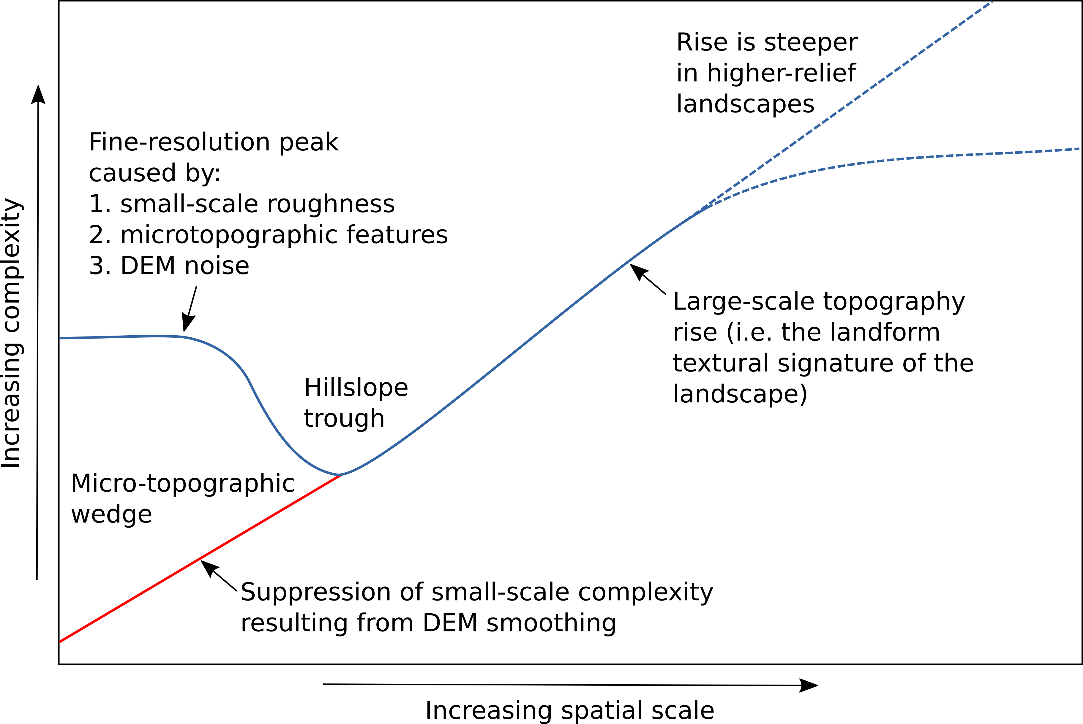
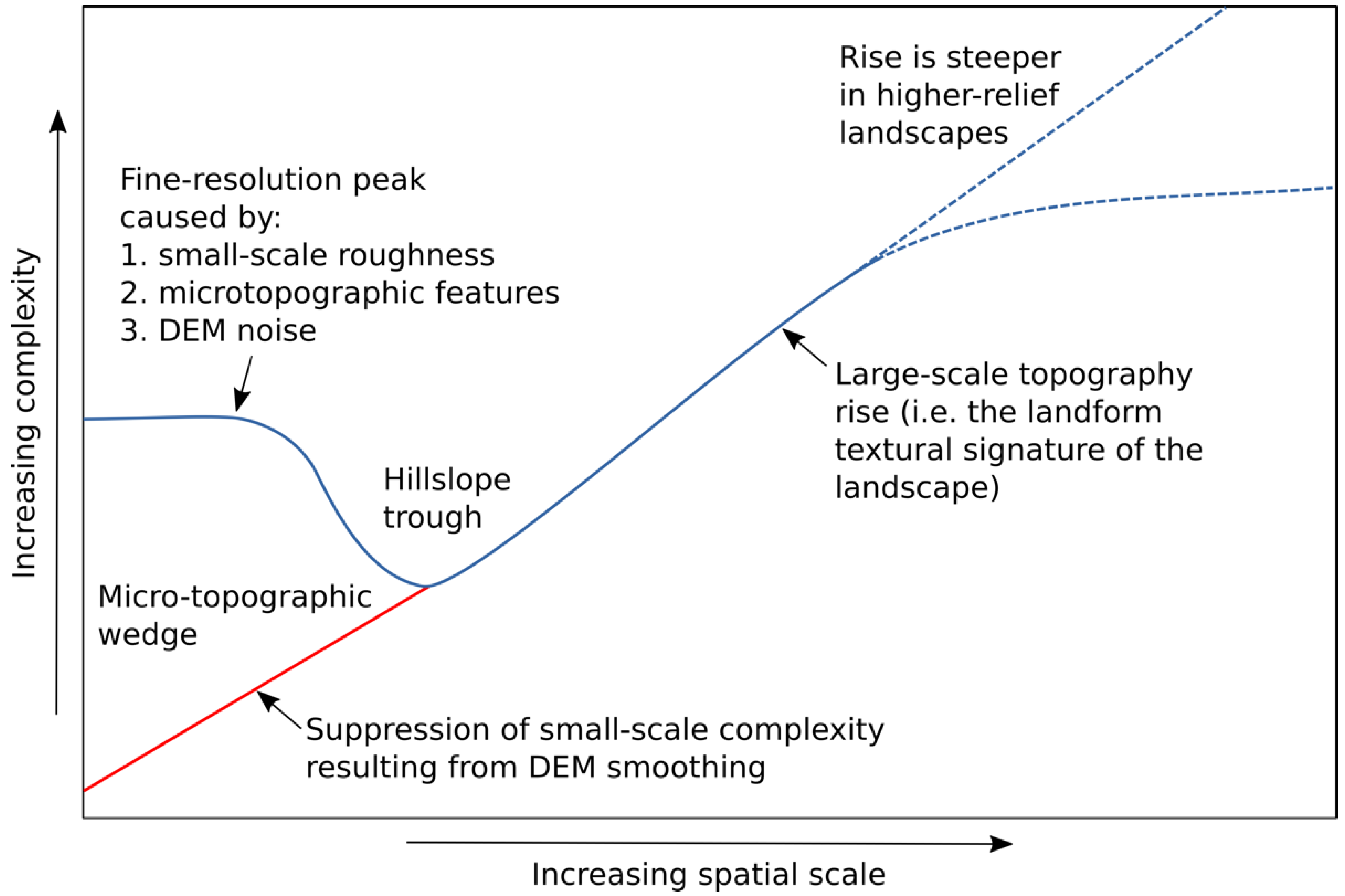
The relation between CVA and kernel size (i.e., spatial scale) is referred to as the CVA scale signature (Figure 3), a function that can be used to characterize the complexity of the topographic surface across spatial scales.
Grohmann et al. [7] found that vector dispersion, which is a measure of angular variance similar to CVA, increases nearly monotonically with increased spatial scale. This was the result of accumulating all of the angular variance of smaller scales up to the test scale. A more revealing scale relation can be estimated by isolating the amount of surface complexity at specific scale ranges. A roughness metric should emphasize the texture of landforms at larger spatial scales, rather than integrating the complexity at all smaller scales. As such, our CVA calculation isolated the surface complexity that was associated with landscape features at a particular test scale by subduing the complexity at smaller scales with an application of Gaussian blur to the DEM.
DEM smoothing methods should aim to reduce the complexity of the surface at the short spatial scales at which roughness dominates, while not significantly altering the topographic complexity at larger spatial scales (Figure 3). The topographic variability at larger spatial scales are dominated by landforms and their representation in DEM should remain unaltered by the DEM smoothing process. Therefore, the CVA scale signature provides a method by which we are able to characterize the impact of a particular smoothing treatment.
3. Results
3.1. FPDEMS Parameter Selection
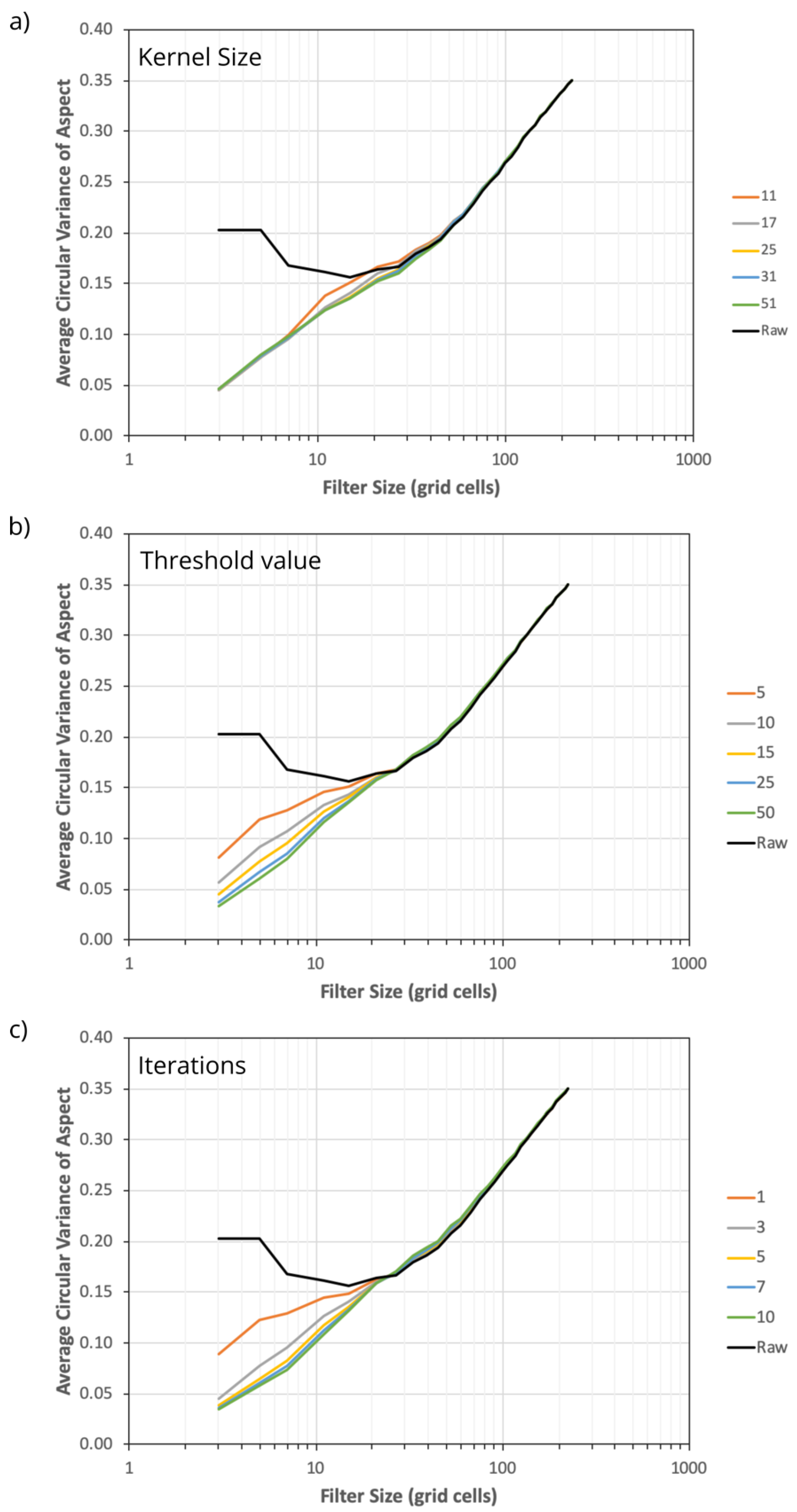
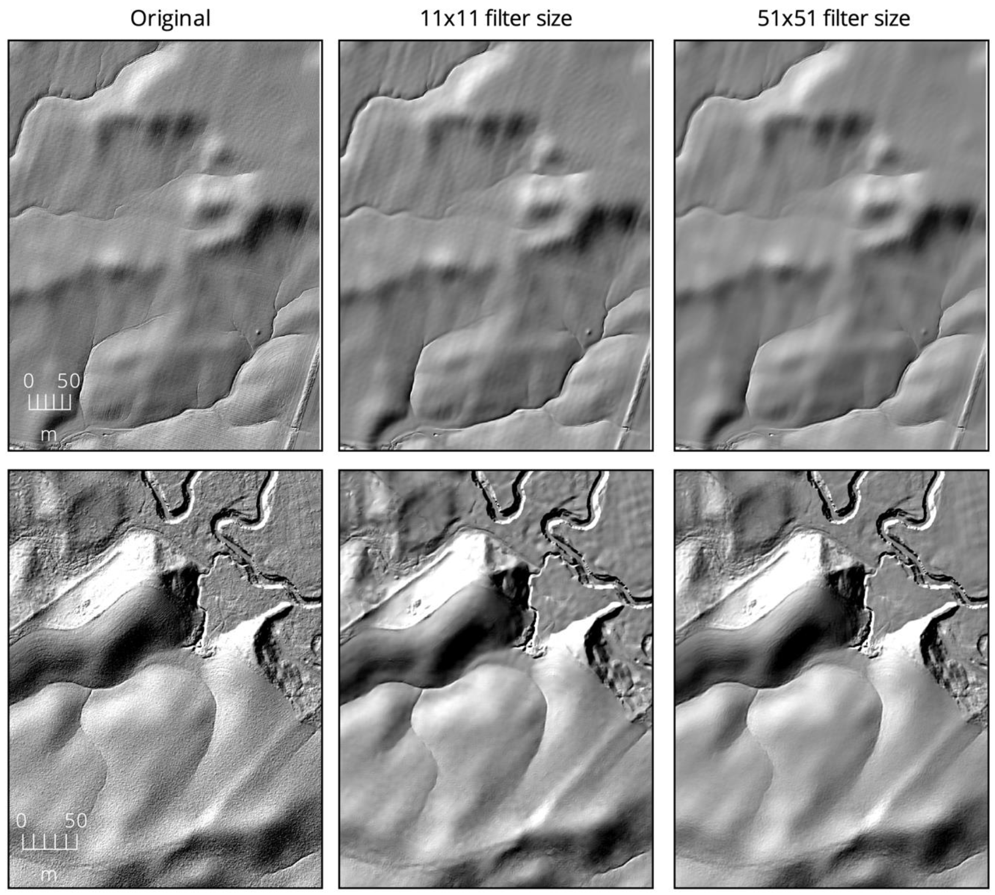
The FPDEMS smoothing method was applied to the study site DEM, with varying parameter settings, while using a computer with a 6-core 2.6 GHz processor and 32 GB of memory. The three main parameters that must be set in the FPDEMS method include the filter kernel size, the normal difference threshold angle, and the number of elevation-update iterations. The method appears to be somewhat insensitive to the choice of filter kernel size, with widely ranging values from 11 × 11 to 51 × 51 providing very similar effects on the CVA scale signatures (Figure 4a). The 11 × 11 test reduced the topographic complexity for a slightly smaller range of scales (Figure 4a), and there was a very small increase in CVA, relative to the untreated DEM, at scales within the hillslope trough (Figure 3). While this would suggest that FPDEMS adds complexity at these intermediate scales, visual examination of the 11 × 11 test DEM (Figure 5) did not reveal any obvious evidence of this (note, shaded relief images are presented, rather than the DEMs, because the subtle differences in topographic texture are more apparent in these data). By filter sizes of 15–17, this phenomenon appears to disappear and the FPDEMS-treated DEMs have CVA signatures that closely follow the original DEM’s signature at intermediate to longer spatial scales. The observed insensitivity to kernel size is likely the result of the weighting scheme that is used in the normal vector smoothing phase of the FPDEMs method. This scheme provides significantly more weight to the neighboring grid cells with similar normal vectors, excluding those cells with normal differences larger than the threshold. Ultimately, this means that, under natural terrain, much of the smoothing weight will be assigned to nearby locations and increasing the kernel size does not provide substantial additional smoothing beyond a certain point (i.e., the point at which the kernels are likely to overlap with adjacent hillslopes, which will be ignored by the thresholding component of the scheme). However, altering the FPDEMS kernel size did significantly impact the processing times when compared with the negligible impact of varying the normal vector difference threshold, and the relatively subdued increase in processing time that was observed with an increased number of elevation-update iterations (Table 1).
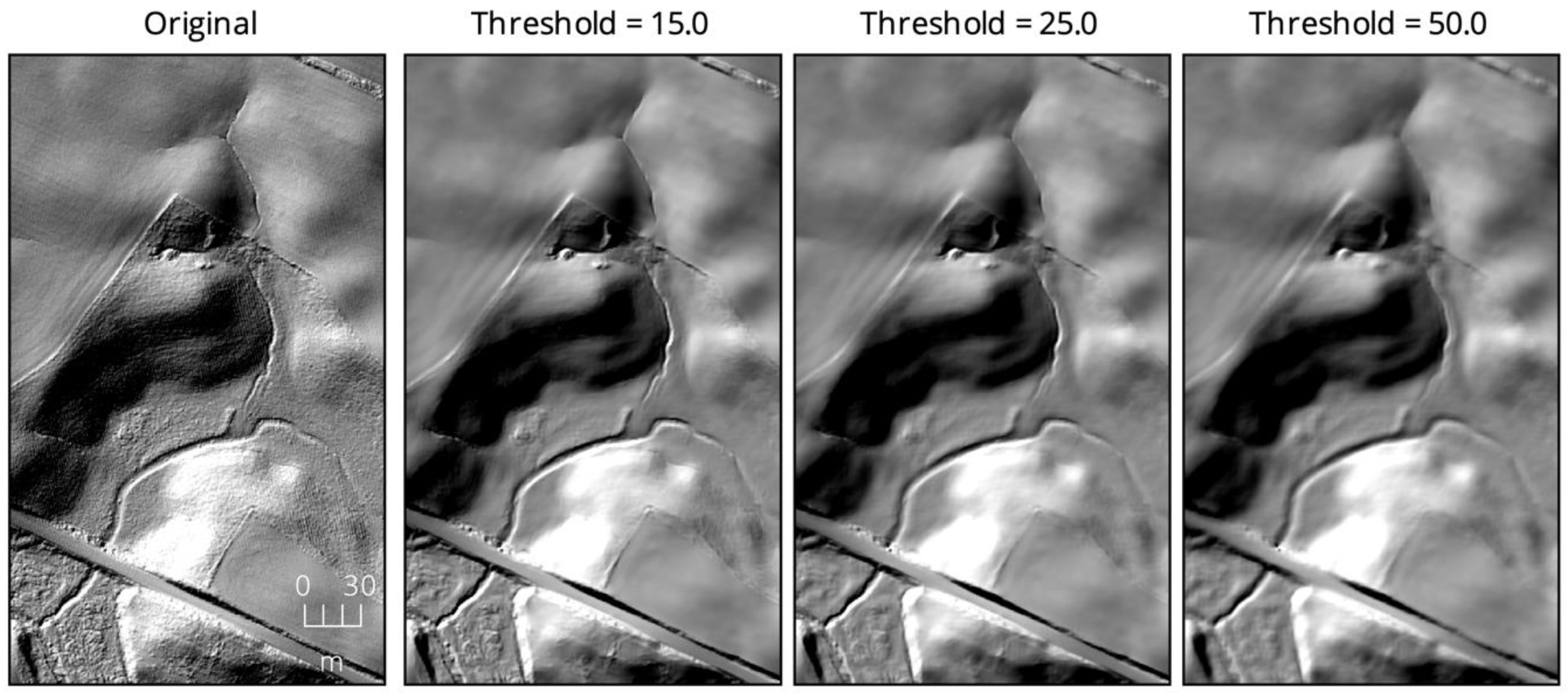
Varying the normal difference threshold angle used in the exclusion of neighboring grid cells situated on different terrain facets (Equation (10)) significantly impacted the extent to which the FPDEMS method smoothed short-scale topographic complexity in the test DEM (Figure 4b). The smallest tested threshold value of 5.0° resulted in far less smoothing than thresholds of 15.0° or higher. At threshold values larger than 15.0°, the CVA scale signatures appear quite similar at all scales. However, the impact of these largest tested threshold values is evident in the resulting smoothed DEMs (Figure 6). While each of the treatments effectively removed short-scale roughness in the DEM, by threshold values of 25° to 50°, the boundaries of channel edges, roadside ditches, and other breaks-in-slope become less sharply defined.
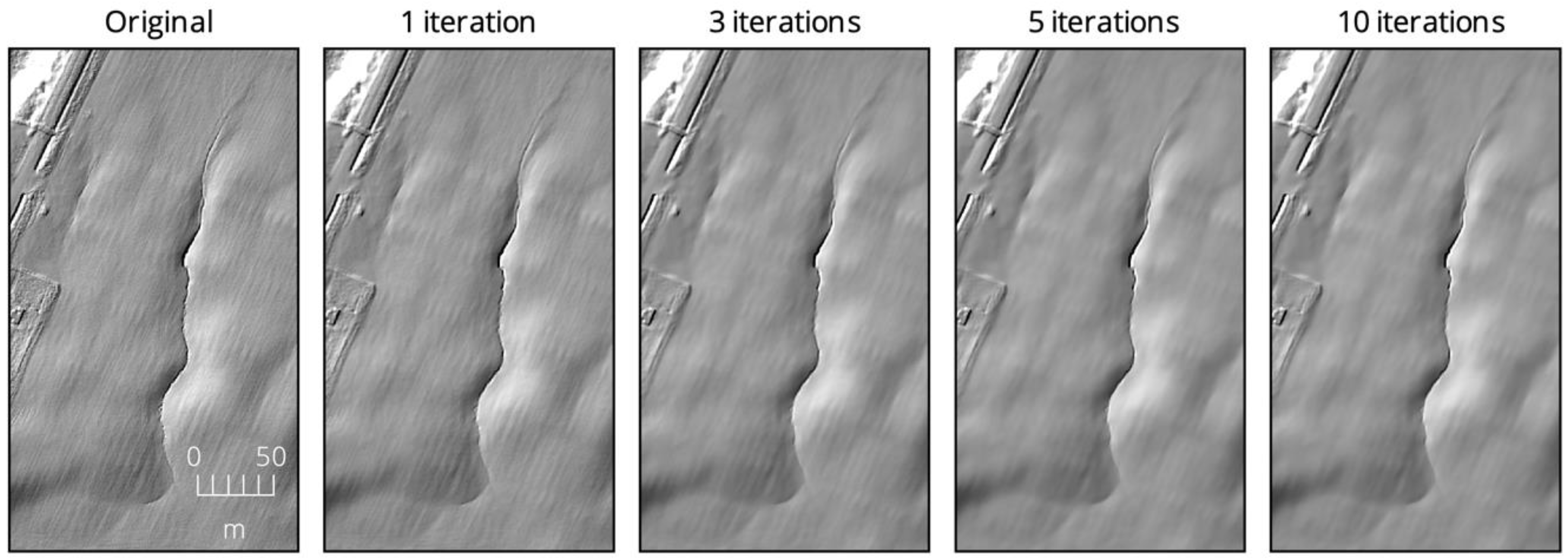
Increasing the number of elevation-update iterations had a similar impact on the CVA scale signature as the effect of altering the normal difference threshold angle (Figure 4c). Increasing from one to three iterations resulted in a significant reduction of short-scale roughness, which widened the micro-topographic wedge (Figure 3). However, further increases in the number of iterations yielded very little change in the resulting scale signatures. This same pattern was also evident from visual inspection of the smoothed DEMs (Figure 7).
Overall, the FPDEMS method produced CVA scale signatures that closely satisfied the ideal of subduing topographic complexity at small spatial scales, while not significantly impacting the complexity of larger-scale landforms (Figure 3). Even with relatively conservative parameter settings (e.g., 11 × 11 kernel, 15° threshold, and three iterations), the method was found to effectively remove the roughness and noise within the DEM. The crispness of significant boundaries was well preserved with threshold values less than approximately 25°, which was particularly evident in the definition of small streams and drainage ditches within the study site. The very slight increase in topographic complexity that was apparent in the CVA signatures at scales between approximately 30 and 60 grid cells (Figure 4) may have resulted from the tendency of the algorithm to not only preserve edge sharpness, but also, under certain parameter settings, to enhance the definition of some rounded boundaries.
3.2. Comparison With Other DEM Smoothing Methods
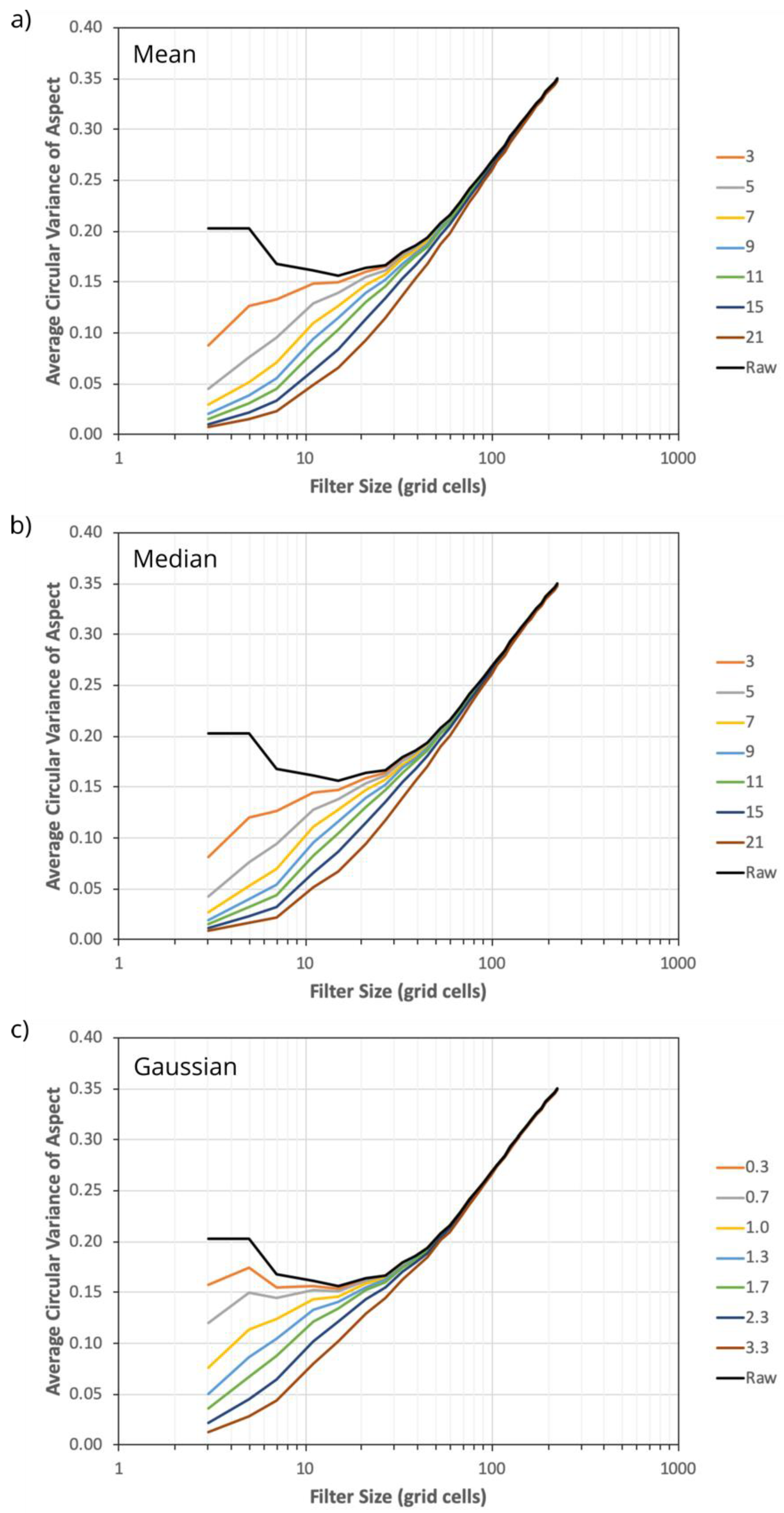
The FPDEMS method was compared with common low-pass filters, including mean, median, and Gaussian filters. The implementations of these filters available in the WhiteboxTools software were used for testing. Varying sized low-pass filters were applied to the study site DEM and the CVA scale signatures were extracted from each of the smoothed DEMs (Figure 8).
The mean, median, and Gaussian low-pass filters showed substantially greater impact at the intermediate to longer spatial scales in their respective CVA scale signatures than the FPDEMS method (Figure 8). Particularly, at the larger tested filter kernel sizes, the signatures documented substantial reductions in the complexity of large-scale topography. It is likely that this was associated with the lowering of peaks/ridges and the raising of valley bottoms/channels at larger kernel sizes of the low-pass filters. The degree to which each of the low-pass filters was able to subdue smaller-scale DEM roughness was also highly dependent on filter kernel size. Significant smoothing was found to occur for the mean and median filters with kernel sizes larger than 7 × 7 and for Gaussian filters with sigma values greater than 1.3–1.7 grid cells. The mean and median CVA scale signatures were very similar overall, while the Gaussian signatures demonstrated more conservative smoothing across all spatial scales at comparable kernel sizes (Figure 8). Of course, this is unsurprising, given the nature of how Gaussian low-pass filters determine kernel weights, providing greater weight to closer neighboring grid cells.
The processing times of all three low-pass filter tests were substantially lower, by approximately one order of magnitude, than those of the corresponding FPDEMS tests (Table 2). The WhiteboxTools mean filter uses an integral-image based approach and the processing times were therefore independent of kernel size. WhiteboxTools’ median filter takes advantage of the redundancy between adjacent filter windows and is therefore also highly efficient. However, the Gaussian filter tests had processing times that approached those of the FPDEMs method, particularly at larger sigma values. All three low-pass filter implementations are parallelized and fully utilized all of the test system’s processor cores.
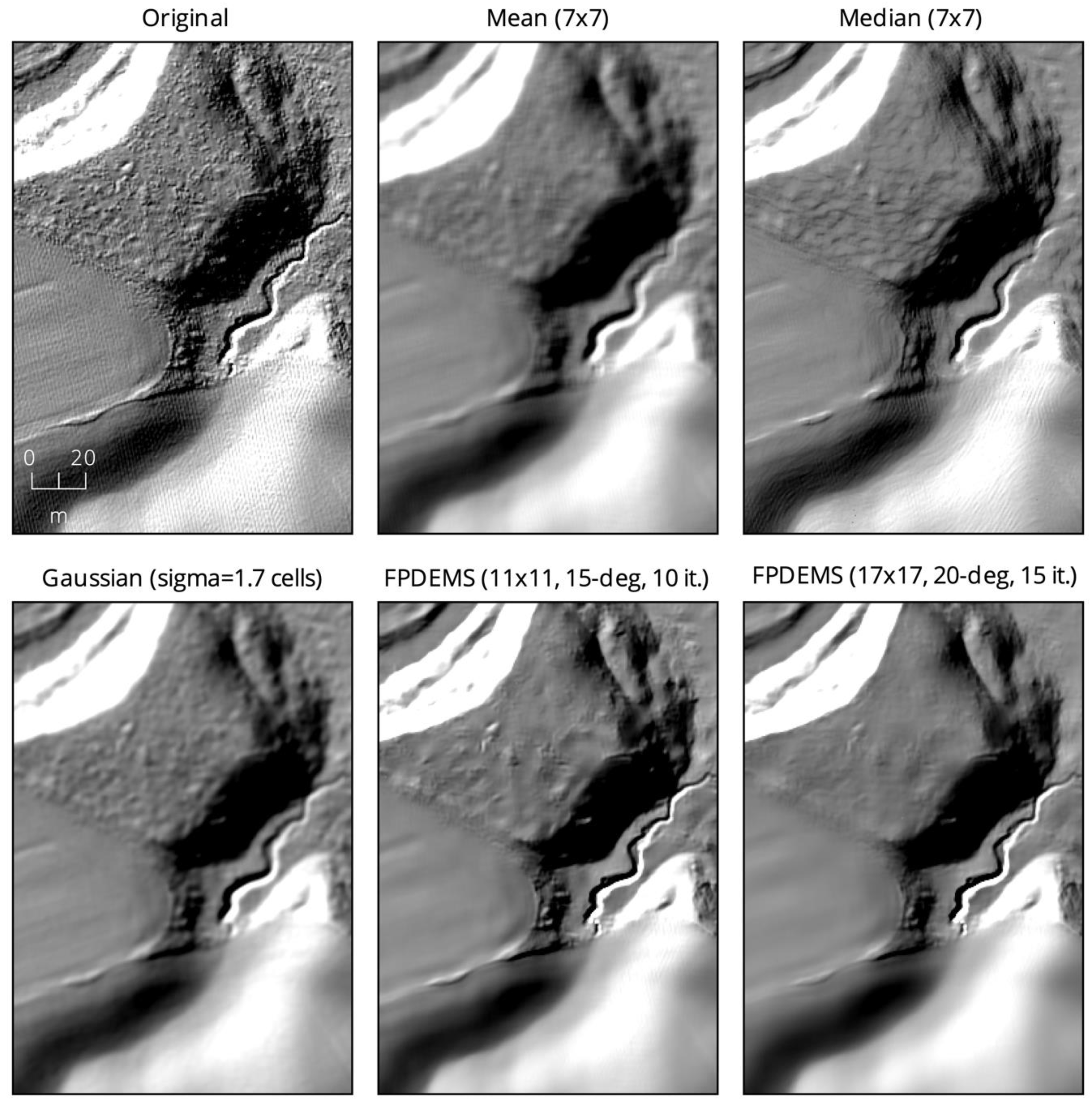
Figure 9 provides a detailed comparison of the impacts of each of the low-pass filters on the study site DEM. This small area within the study site shows portions of two agricultural fields (lower half) and a forested area (upper half). While the trees of the forested areas are not present in the DEM, the excessive roughness of the forest floor is apparent in the unsmoothed data set. A steep terrace scarp is apparent in the bright section within the upper-left corner of the image, and the boundaries of this slope are well defined (Figure 9). A deep, steep-sided gully, initiating at the field-forest edge and within the swale between the two fields, cuts through the central area. Tillage patterns and DEM noise (nearly vertical striping possibly due to LiDAR scan lines) are also evident within the gentler topography of the fields.
The mean and Gaussian filters both notably blur the edges of the hillslope and gully features. The complex texture of the fields is effectively removed while using both of these filters; however, significant roughness remains within the forested areas (Figure 9). The median filter, by comparison, does well to preserve the sharpness of the breaks-in-slope, while also smoothing the roughness of the original DEM. Nonetheless, the shape of the gully does appear to be significantly altered by median filtering; the narrow end-portion of the feature is filled in and the middle section appears to be widened. However, perhaps more problematic is the introduction of a contouring effect that is particularly apparent on the steeper forested areas and within the lower field swale. These small terrace-like features, which resemble slump scars, are not evident within the original DEM. Based on the CVA scale signatures (Figure 8) and the inspection of the filtered DEMs, it is apparent that smaller filter kernel sizes would result in substantially more retained roughness after smoothing and larger kernels would yield more edge blurring (mean and Gaussian filters) or more alteration of feature shapes and artificial terracing (median filter).
Figure 9 presents two FPDEMS method treatments (11 × 11 kernel/15° threshold/10 iterations and 17 × 17 kernel/20° threshold/15 iterations) for comparison with the common low-pass techniques. The edge-preserving nature of FPDEMS is clearly able to maintain the sharp breaks-in-slope that is associated with the gully and the terrace scarp. Furthermore, the shape of the gully feature does not appear to be significantly altered by the treatments with the FPDEMS method. Both of the treatments appear to remove the texture of the original DEM within the fields. The less aggressive FPDEMS smoothing treatment (11 × 11 kernel/15° threshold/10 iterations) did as well or better at removing the excessive roughness of the forested areas than the three low-pass filters. The more aggressive treatment was able to remove almost all of the roughness of the forest floors, albeit with some loss in finer topographic details, e.g., the hedge-row mound dividing the two fields was smoothed.
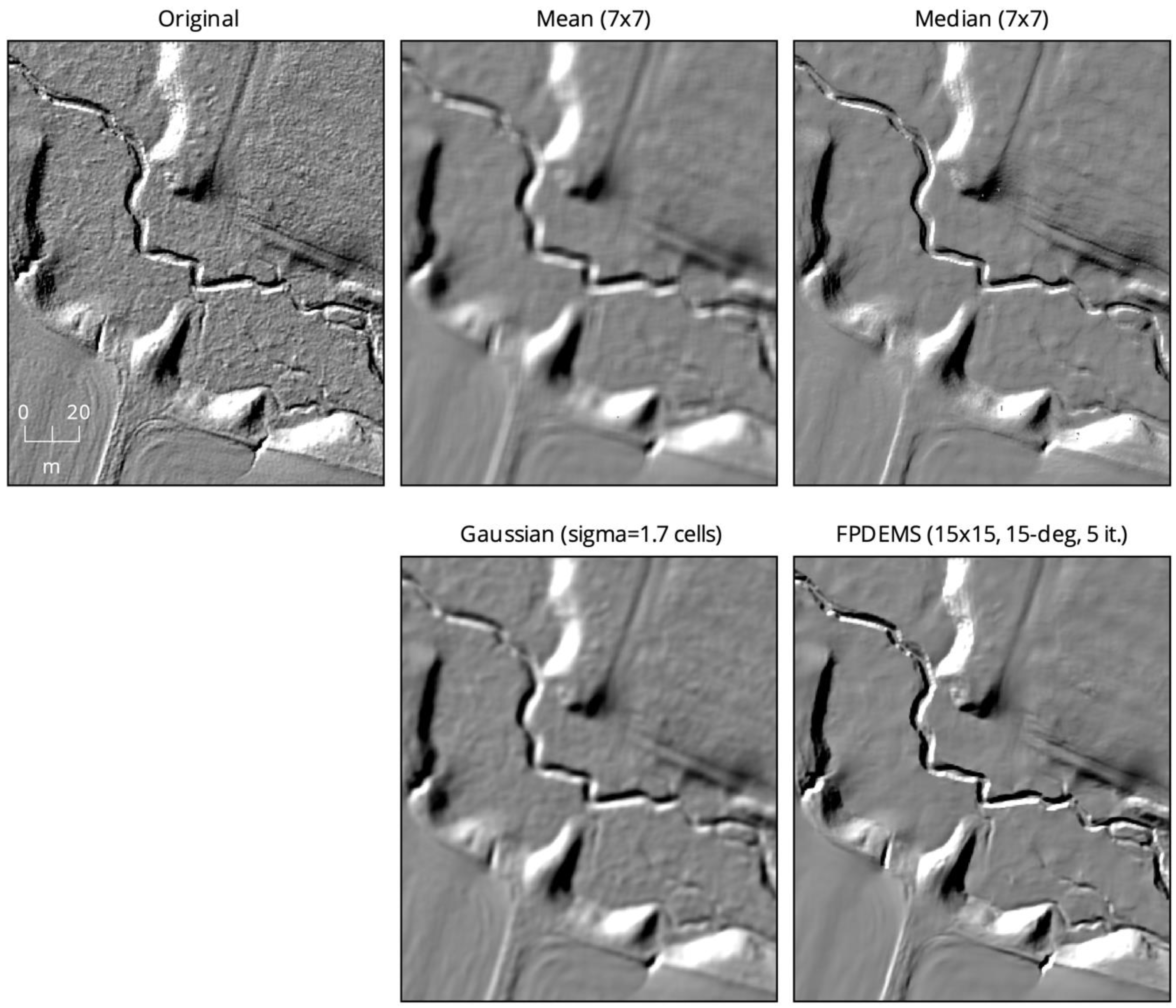
In addition to preserving the sharpness of breaks-in-slope, the FPDEMS method was particularly well suited to maintaining the geometry of the small streams and other drainage features (e.g., roadside ditches). Figure 10 shows the effects of each of the tested smoothing methods in an area containing a deeply incised stream channel. The mean and Gaussian filters both rounded the channel banks, widened the channel, and raised the bottom, effectively filling in the feature in narrower places. By comparison, the median low-pass filter and FPDEMS method preserved the steepness of channel banks well. However, notice how the yazoo tributary that flows along the bottom of the southern terrace scarp (lower right corner) is retained after treatment with the FPDEMS method, but it is obscured by the median filtering treatment.
Although the CVA scale signatures quantify the impact of treatment methods on the topographic complexity at different scales, and the shaded-relief images provide a means to visually characterize the impact of treatments on specific features, it is also useful to examine the relative degree to which treatments modify the original DEM. The root-mean-square (RMS) elevation differences between the mean (7 × 7), median (7 × 7), Gaussian (Sigma = 1.7 cells), and FPDEMS (11 × 11 kernel/15° threshold/10 iterations) treated DEMs and the original data were 0.082 m, 0.048 m, 0.069 m, and 0.028 m, respectively, and the 90% linear error (LE90) values were 0.056 m, 0.048 m, 0.048 m, and 0.043 m, respectively. Therefore, for similar overall levels of smoothing (Figure 4 and Figure 8), the FPDEMS method requires less overall modification of the original elevation values.
3.3. Implications For Flow-Path Modelling
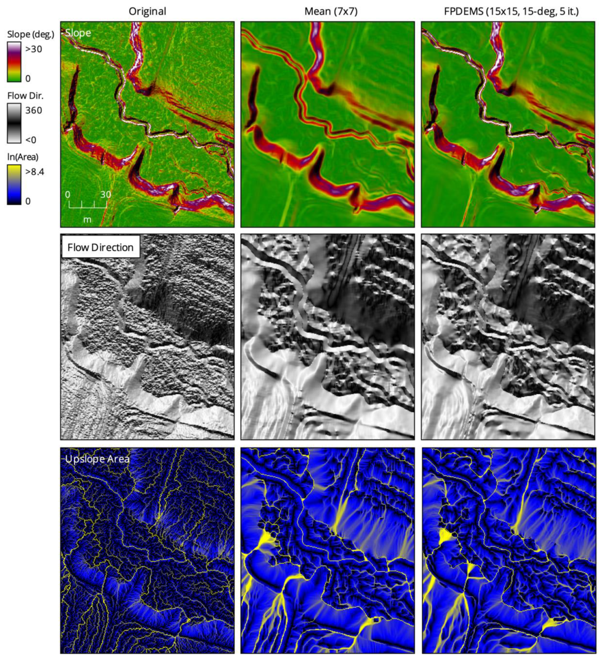
The earlier sections demonstrate the ability of the FPDEMS method to subdue the roughness that often impact DEM-based surface flow-path modelling, while also preserving the small drainage features, such as headwater streams and ditches, which are apparent in LiDAR data. It is frequently the effects that excessive roughness has on the ability to model flow patterns while using a DEM that are the primary motivation for smoothing LiDAR data. Flow-path modelling relies on the accurate characterization of local slope gradient and flow direction (related to aspect), which in turn may be used to model the flow pathways and the spatial pattern of upslope area (Figure 11). These data are applied in delineating catchments and in modelling soil moisture (e.g., the wetness index) and sediment erosion and transport.
A comparison of the effects of mean filtering and the FPDEMS method on flow-path modelling data (Figure 11) demonstrated the impact that even a relatively small 7 × 7 mean filtering has on the slope distribution. The slope gradient along the banks of the incised channel is significantly reduced. Similarly, the steepest portions of the terrace scarps are also somewhat flattened by mean filtering. The FPDEMS method, by comparison, preserves the steepest slope gradients along both the incised channel and the terrace scarps, while subduing the slope variability resulting from micro-topographic roughness. The range of slope values after applying the FPDEMS method (0.0° to 58.8°) was similar to the original DEM (0.0° to 60.1°), while mean filtering substantially reduced the range (0.0° to 48.5°).
The effects of roughness in the original LiDAR DEM are probably most apparent in the D∞ [37] flow direction data (Figure 11), where the larger-scale flow patterns are completely overwhelmed by local-scale variability. The irregularity of modelled flow directions, due to excessive roughness, has the effect of lengthening flow paths, which are apparent in the convoluted flow lines in the upslope area data. The mean filter and the FPDEMS treatments were both found to effectively suppress the local-scale signal in flow-directions, providing for clearer representation of field-scale surface flow patterns. The shallowing of the bank slopes and widening of the channel by the mean filter noted above is also apparent in the flow direction data, as is the relative sharpness of major breaks-in-slope in the FPDEMS flow direction image. However, the difference between the two DEM smoothing techniques are less pronounced in the D∞-derived [37] upslope area (i.e., flow accumulation) data. Both techniques significantly and similarly impacted the pattern of upslope area, providing shorter, less convoluted flow pathways and more divergent flow patterns on the hillslopes (denoted by the fuzzier appearance of the smoothed upslope area rasters in Figure 11), as compared to the original DEM. While visual interpretation of these smoothed flow patterns is arguably improved by the treatments, it is difficult to comment on the accuracy of one distribution over another in the absence of reference data. Researchers often assess the accuracy of flow patterns while using mapped stream networks; however, in this area, the mapped streams are of a lower spatial accuracy than the LiDAR data.
While comparisons with the median and Gaussian filter treatments are not provided in Figure 11, their impacts were observed to be intermediary between those of the mean and FPDEMS treatments. Instead we have chosen to compare the relative impact of the FPDEMS method with the mean filter for brevity, because the mean treatment provides the greatest contrast with the FPDEMS method, and because of the common use of mean filtering for DEM smoothing in practice.
4. Discussion
The CVA scale signatures show that the FPDEMS method exhibits the desired property of subduing the micro-topographic peak by smoothing roughness and reducing noise in fine-resolution LiDAR data when applied with filter kernel sizes larger than 11 × 11, normal difference threshold angles of larger than 15°, and with three or more elevation-update iterations (Figure 4). Threshold angles of between approximately 10° and 20° were found to be optimal for the test data, with threshold values that were larger than this producing a loss of definition in the incised channel banks and terrace scarp boundaries within the site. This range of threshold values is narrower than the 8.1° to 29.5° range recommended by Stevenson et al. [13] when applying the Sun et al.’s [31] method to coarser-resolution interferometric DEMs.
The low-pass filter methods produced CVA scale signatures that showed greater alteration, specifically a lowering of topographic complexity, at broader spatial scales extending upwards of about 100 grid cells (Figure 8). This was particularly obvious for filter kernel sizes that were larger than about nine grid cells (mean and median filters) and for sigma values larger than 2.3 grid cells (Gaussian filter). Naturally, the lowering of peaks and divides and the raising of channels and valley floors that were caused by spatial elevation averaging caused this decrease in the average CVA at these scales. The FPDEMS treated elevation models produced CVA signatures that consistently, being insensitive to parameter settings, more closely matched the signature of the original DEM at broader spatial scales. However, under certain parameter settings, the method did produce signatures that exhibited a small increase in average CVA at intermediate scales. Any increase in average CVA is unexpected because it implies that the smoothing technique has introduced topographic complexity at these scales. We hypothesize that this introduced complexity may have resulted from the tendency of the method, at smaller filter kernel sizes and with greater elevation-update iterations, to enhance the sharpness of the originally rounded slopes. That is, while the method does well to preserve the original sharpness of natural breaks-in-slope, under some conditions it did tend to produce a sharper break than what appeared in the original DEM. This phenomenon was not widespread in the test data, but it is the reason that kernel sizes less than 11 × 11 grid cells and greater than 15 elevation-update iterations are not recommended for application with fine-resolution LiDAR data such as those used in the test.
While the computational performance of the FPDEMS method was substantially lower than the conventional low-pass filter techniques, processing times were found to be practically reasonable for general application with typical LiDAR data sets. The 1.3 GB study site DEM was smoothed while using the FeaturePreservingSmoothing tool in between 2.6 and 22.4 minutes, depending on the parameter settings. This indicates that the method can be practically applied to the types and sizes of LiDAR DEMs that are commonly applied in research at present. The processing times were particularly sensitive to the filter kernel size parameter, although the impact of varying this parameter on the degree of smoothing was significantly less than either the normal difference threshold angle or the number of elevation-update iterations. Thus, it is recommended that, when applied to fine-resolution LiDAR data sets, filter kernels of between 11 and 21 grid cells are best. While comparisons were made with the low-pass filters that are commonly used for DEM smoothing in practice, it would have also been useful to compare the FeaturePreservingSmoothing tool against other feature-preserving methods. Unfortunately, we were unable to successfully apply either GRASS GIS’s r.denoise tool or SAGA GIS’s Mesh Denoise tool to the study site DEM. Mesh Denoise’s memory use continued to increase during operation and the process was terminated after more than three hours. The Mesh Denoise tool relied heavily on slow virtual memory and was terminated when the memory requirements of the tool were approximately five times the available system memory. By comparison, the FeaturePreservingSmoothing tool required a maximum 6.04 GB of memory.
The application of CVA scale signatures provided a useful means of assessing the impact of various smoothing methods, and of varying parameter settings, on the topographic information contained within the DEM. It allowed for the quantification of the degree to which a treatment successfully subdued micro-topographic roughness and DEM noise without altering longer-range topographic features, including landform representation. It is important to note that the hillslope trough of the CVA scale signature (Figure 3) is not a direct measure of the average hillslope length scale of the site, but is related to it. The trough results from a filter kernel size that is larger than the scale at which micro-topographic roughness and noise are expressed and is small enough that a significant number of filter windows will not overlap with adjacent terrain facets separated by divides or valley bottoms. Filter windows that are completely contained within a single hillslope will exhibit a relatively uniform aspect, since hillslopes are defined by their characteristic slope orientation (while gradients may vary downslope). For the study site that was examined in this research, this scale of suppressed topographic complexity was relatively short and it extended from approximately 7 to 30 grid cells (3.5 to 15 m). More rugged terrains are likely to exhibit CVA signature troughs at longer scales, and perhaps possess broader-shaped hillslope troughs.
The edge-preserving nature of the FPDEMS method performed better at retaining the sharp definition of significant breaks-in-slope within the test DEM, as compared with mean and Gaussian filtering. Median filtering offered a similar level of edge-preservation to the FPDEMS method; however, it exhibited the undesirable qualities of changing the shape of features and introducing an artificial contouring to the data. Sun et al. [31] also noted the characteristic of median-based filtering to introduce artifact features in noisy 3D meshes. When compared with the low-pass filters, the FPDEMS did not appreciably fill-in, widen, or alter the shape of the incised streams that were found throughout the study site. It also performed better in retaining the small in-field headwater channels, gullies, and the roadside ditches that were common within the site. The extra costs of acquiring LiDAR data are often motivated by the ability of these data to better represent these types of small-scale drainage features [38]. Many of these drainage features occupy similar spatial scales to the roughness within LiDAR data and this research demonstrates that some of the most commonly applied DEM smoothing techniques can significantly degrade their representations.
The spatial distribution of slope that was produced by the FPDEMS method was simplified by removing short-scale variation in the original DEM, without altering large-scale patterns or shortening the overall range of slope values. As with mean filtering, flow-direction data were found to be significantly simplified through the application of the FPDEMS method, providing less convoluted flow paths. While the simplified flow-direction raster is certainly easier to visually interpret than the pattern that is produced by the rough DEM, whether or not this is more realistic is likely a function of the type of flow phenomena operating in an area. The more convoluted flow paths that are dominated by the excessive roughness in the original DEM may better reflect overland flow patterns, particularly across tilled agricultural fields where tillage and rills are known to control flow [39,40]. However, in places where shallow subsurface flow dominates runoff processes, the smoothed flow directions and more divergent pathways provided by the mean filter and FPDEMS method may better represent the flow patterns at the field-scale. Drainage channels exist because the magnitude and frequency of flow allows for the erosion and transportation of sediment within to outpace the rate of deposition [41]. Thus, the preservation of small-scale drainage features in a DEM after smoothing, such as that demonstrated by the FPDEMS method, must provide a more realistic model of local flow patterns than a DEM in which these features have been completely obscured by either liberal, non-edge-preserving smoothing or data resampling.
5. Conclusions
Fine-resolution LiDAR data are often characterized by very high surface roughness. This local-scale variability can greatly impact the ability of researchers to quantify topographic shape (e.g., slope, aspect, curvature) and to model the near-surface flow processes. DEM smoothing methods, such as low-pass filtering and data resampling, are often applied to LiDAR DEMs as a pre-processing step to overcome these challenges. Unfortunately, these techniques can negatively impact the representation of topographic features, most notably drainage features, like headwater streams and ditches. Previous research has demonstrated the potential for using normal vector field smoothing as the basis for feature-preserving DEM generalization. This paper presented a novel DEM smoothing technique, called FPDEMS, which was implemented as the FeaturePreservingSmoothing tool of the WhiteboxTools geospatial analysis software. The FPDEMS method is based on a feature-preserving normal vector field smoothing technique that is similar to Sun et al.’s [31] approach, originally designed for de-noising 3D meshes. However, the FPDEMS method has been optimized for application with large raster DEMs.
The suitability of the FPDEMS method for smoothing a LiDAR DEM of a largely agricultural area in southwestern Ontario, Canada was evaluated by comparing its performance against commonly applied low-pass filters. The findings demonstrated that the technique performed better at removing DEM roughness, while preserving the sharpness of breaks-in-slope and retaining small drainage features, as compared with mean, median, and Gaussian filters. Optimal parameter values for application with the LiDAR data set occurred with kernel sizes of between 11 and 21 grid cells, threshold angles (used for normal vector field smoothing) of 10° to 20°, and three to 15 elevation-update iterations. These settings allowed for an effective reduction in micro-topographic roughness and DEM noise and the retention of terrace scarp boundaries, incised channel banks, gullies, and headwater streams.
Author Contributions
Conceptualization, J.B.L. and A.F.; methodology, J.B.L., A.F. and J.M.H.C.; software, J.B.L.; validation, J.B.L.; formal analysis, J.B.L.; investigation, J.B.L. and A.F.; resources, J.B.L.; data curation, J.B.L.; writing—original draft preparation, J.B.L.; writing—review and editing, J.B.L., A.F. and J.M.H.C.; visualization, J.B.L.; supervision, J.B.L. and J.M.H.C.; project administration, J.B.L.; funding acquisition, J.B.L.
Funding
This research was funded by a grant provided by the Natural Sciences and Engineering Research Council of Canada (NSERC; grant number 400317).
Acknowledgments
The authors would like to thank the contributions of the anonymous reviewers.
Conflicts of Interest
The authors declare no conflict of interest. The funders had no role in the design of the study; in the collection, analyses, or interpretation of data; in the writing of the manuscript, or in the decision to publish the results.
References
- Baltsavias, E.P. A comparison between photogrammetry and laser scanning. Isprs J. Photogramm. Remote Sens. 1999, 54, 83–94. [Google Scholar] [CrossRef]
- Hodgson, M.E.; Bresnahan, P. Accuracy of airborne lidar-derived elevation. Photogramm. Eng. Remote Sens. 2004, 70, 331–339. [Google Scholar] [CrossRef]
- Yang, P.; Ames, D.P.; Fonseca, A.; Anderson, D.; Shrestha, R.; Glenn, N.F.; Cao, Y. What is the effect of LiDAR-derived DEM resolution on large-scale watershed model results? Environ. Model. Softw. 2014, 58, 48–57. [Google Scholar] [CrossRef]
- Brubaker, K.M.; Myers, W.L.; Drohan, P.J.; Miller, D.A.; Boyer, E.W. The use of LiDAR terrain data in characterizing surface roughness and microtopography. Appl. Environ. Soil Sci. 2013, 2013, 1–13. [Google Scholar] [CrossRef]
- MacMillan, R.A.; Martin, T.C.; Earle, T.J.; McNabb, D.H. Automated analysis and classification of landforms using high-resolution digital elevation data: applications and issues. Can. J. Remote Sens. 2003, 29, 592–606. [Google Scholar] [CrossRef]
- Lindsay, J.B.; Creed, I.F. Sensitivity of digital landscapes to artifact depressions in remotely-sensed DEMs. Photogramm. Eng. Remote Sens. 2005, 71, 1029–1036. [Google Scholar] [CrossRef]
- Grohmann, C.H.; Smith, M.J.; Riccomini, C. Multiscale analysis of topographic surface roughness in the Midland Valley, Scotland. IEEE Trans. Geosci. Remote Sens. 2010, 49, 1200–1213. [Google Scholar] [CrossRef]
- Lindsay, J.B.; Newman, D.R. Hyper-scale analysis of surface roughness. Peer J Prepr. 2018, 6, e27110v1. [Google Scholar]
- Reuter, H.I.; Hengl, T.; Gessler, P.; Soille, P. Chapter 4 Preparation of DEMs for geomorphometric analysis. Dev. Soil Sci. 2009, 33, 87–120. [Google Scholar]
- Habtezion, N.; Tahmasebi Nasab, M.; Chu, X. How does DEM resolution affect microtopographic characteristics, hydrologic connectivity, and modelling of hydrologic processes? Hydrol. Process. 2016, 30, 4870–4892. [Google Scholar] [CrossRef]
- Deng, Y.; Wilson, J.P.; Bauer, B.O. DEM resolution dependencies of terrain attributes across a landscape. Int. J. Geogr. Inf. Sci. 2007, 21, 187–213. [Google Scholar] [CrossRef]
- Tian, B.; Wang, L.; Koike, K. Spatial statistics of surface roughness change derived from multi-scale digital elevation models. Procedia Environ. Sci. 2011, 7, 252–257. [Google Scholar] [CrossRef] [Green Version]
- Stevenson, J.A.; Sun, X.; Mitchell, N.C. Despeckling SRTM and other topographic data with a denoising algorithm. Geomorphology 2010, 114, 238–252. [Google Scholar] [CrossRef]
- Zakšek, K.; Podobnikar, T. An effective DEM generalization with basic GIS operations. In Proceedings of the 8th ICA WORKSHOP on Generalisation and Multiple Representation, A Coruńa, Spain, 7–8 July 2005; the International Cartographic Association (ICA): Bern, Switzerland, 2005; p. 10. [Google Scholar]
- Lindsay, J.B. Whitebox GAT: A case study in geomorphometric analysis. Comput. Geosci. 2016, 95, 75–84. [Google Scholar] [CrossRef]
- Grohmann, C.H. Effects of spatial resolution on slope and aspect derivation for regional-scale analysis. Comput. Geosci. 2015, 77, 111–117. [Google Scholar] [CrossRef] [Green Version]
- Chen, Y.; Wilson, J.P.; Zhu, Q.; Zhou, Q. Comparison of drainage-constrained methods for DEM generalization. Comput. Geosci. 2012, 48, 41–49. [Google Scholar] [CrossRef]
- Chen, Y.; Zhou, Q. A scale-adaptive DEM for multi-scale terrain analysis. Int. J. Geogr. Inf. Sci. 2013, 27, 1329–1348. [Google Scholar] [CrossRef]
- Ai, T.; Li, J. A DEM generalization by minor valley branch detection and grid filling. Isprs J. Photogramm. Remote Sens. 2010, 65, 198–207. [Google Scholar] [CrossRef]
- Walker, J.P.; Willgoose, G.R. On the effect of digital elevation model accuracy on hydrology and geomorphology. Water Resour. Res. 1999, 35, 2259–2268. [Google Scholar] [CrossRef] [Green Version]
- Gallant, J. Adaptive smoothing for noisy DEMs. In Proceedings of the Geomorphometry 2011, Redlands, CA, USA, 7–8 September 2011. [Google Scholar]
- Barash, D. A fundamental relationship between bilateral filtering, adaptive smoothing, and the nonlinear diffusion equation. IEEE Trans. Pattern Anal. Mach. Intell. 2002, 26, 844–847. [Google Scholar] [CrossRef]
- Usul, N.; Pasaogullari, O. Effect of map scale and grid size for hydrological modelling. Iahs Publ. 2004, 289, 91–100. [Google Scholar]
- Petrasova, A.; Mitasova, H.; Petras, V.; Jeziorska, J. Fusion of high-resolution DEMs for water flow modeling. Open Geospat. Datasoftware Stand. 2017, 2, 6. [Google Scholar] [CrossRef]
- Harwood, D.; Subbarao, M.; Hakalahti, H.; Davis, L.S. A new class of edge-preserving smoothing filters. Pattern Recognit. Lett. 1987, 6, 155–162. [Google Scholar] [CrossRef]
- Tomasi, C.; Manduchi, R. Bilateral filtering for gray and color images. Proc. Iccv 1998, 98, 2. [Google Scholar]
- Paris, S.; Kornprobst, P.; Tumblin, J.; Durand, F. Bilateral filtering: Theory and applications. Found. Trends® Comput. Graph. Vis. 2009, 4, 1–73. [Google Scholar] [CrossRef]
- Fleishman, S.; Drori, I.; Cohen-Or, D. Bilateral mesh denoising. ACM 2003, 22, 950–953. [Google Scholar]
- Jones, T.R.; Durand, F.; Desbrun, M. Non-iterative, feature-preserving mesh smoothing. ACM 2003, 22, 943–949. [Google Scholar] [Green Version]
- Lee, K.-W.; Wang, W.-P. Feature-preserving mesh denoising via bilateral normal filtering. In Proceedings of the Ninth International Conference on Computer Aided Design and Computer Graphics (CAD-CG’05), Hong Kong, China, 7–10 December 2005; IEEE: Washington, DC, USA, 2005. [Google Scholar]
- Sun, X.; Rosin, P.L.; Martin, R.; Langbein, F. Fast and effective feature-preserving mesh denoising. IEEE Trans. Vis. Comput. Graph. 2007, 13, 925–938. [Google Scholar] [CrossRef]
- Zheng, Y.; Fu, H.; Au, O.K.-C.; Tai, C.-L. Bilateral normal filtering for mesh denoising. IEEE Trans. Vis. Comput. Graph. 2010, 17, 1521–1530. [Google Scholar] [CrossRef]
- Horn, B.K. Hill shading and the reflectance map. Proc. IEEE 1981, 69, 14–47. [Google Scholar] [CrossRef] [Green Version]
- Lindsay, J.B. WhiteboxTools User Manual. Available online: https://jblindsay.github.io/wbt_book/preface.html (accessed on 16 August 2019).
- Chapman, L.J.; Putnam, D.F. Physiography of Southern Ontario; University of Toronto Press: Toronto, ON, Canada, 1973; p. 284. [Google Scholar]
- MNRF User Guide: Lidar Point Cloud (2016-18) LIO Dataset v. 1.3. Available online: https://www.sse.gov.on.ca/sites/MNR-PublicDocs/EN/CMID/Lidar%20Point%20Cloud%20-%20User%20Guide.pdf (accessed on 16 August 2019).
- Tarboton, D.G. A new method for the determination of flow directions and upslope areas in grid digital elevation models. Water Resour. Res. 1997, 33, 309–319. [Google Scholar] [CrossRef] [Green Version]
- James, L.A.; Watson, D.G.; Hansen, W.F. Using LiDAR data to map gullies and headwater streams under forest canopy: South Carolina, USA. Catena 2007, 71, 132–144. [Google Scholar] [CrossRef]
- Govers, G.; Takken, I.; Helming, K. Soil roughness and overland flow. Agronomie 2000, 20, 131–146. [Google Scholar] [CrossRef]
- Govers, G.; Giménez, R.; Van Oost, K. Rill erosion: exploring the relationship between experiments, modelling and field observations. Earth-Sci. Rev. 2007, 84, 87–102. [Google Scholar] [CrossRef]
- Montgomery, D.R.; Dietrich, W.E. Source areas, drainage density, and channel initiation. Water Resour. Res. 1989, 25, 1907–1918. [Google Scholar] [CrossRef] [Green Version]
Figure 1.
Scheme used to denote the address of the eight elevation values surrounding grid cell, zi,j, in a raster digital elevation model (DEM). The DEM grid resolution, d, is the spacing between neighboring cells.
Figure 1.
Scheme used to denote the address of the eight elevation values surrounding grid cell, zi,j, in a raster digital elevation model (DEM). The DEM grid resolution, d, is the spacing between neighboring cells.

Figure 2.
The study site located northeast of Brantford, within Southwestern Ontario, Canada. The 0.5 m resolution DEM is displayed here with shaded relief to emphasize topographic variation.
Figure 2.
The study site located northeast of Brantford, within Southwestern Ontario, Canada. The 0.5 m resolution DEM is displayed here with shaded relief to emphasize topographic variation.

Figure 3.
A conceptual model of the impact of an ideal DEM smoothing treatment on the CVA scale signature. The blue line represents the pattern of circular variance of aspect (CVA) for a hypothetical DEM and the red line indicates the effects of an ideal smoothing treatment. That is, smoothing should result in suppression of surface complexity at shorter scales while leaving larger scale complexity unaffected.

Figure 4.
The effects of Feature Preserving DEMs (FPDEMs) smoothing on the CVA scale signature of the study site DEM including varying (a) the filter kernel size from 11 × 11 to 51 × 51 (in grid cells; each test used a threshold of 15° and three iterations), (b) the normal vector difference threshold from 5° to 50° (each test used 17 × 17 kernels and three iterations), and (c) the number of elevation-update iterations from 1 to 10 (each test used 17 × 17 kernels and a threshold of 15°).

Figure 5.
The effect of altering the FPDEMs filter size for two small areas within the study DEM. Each smoothing operation was run with a normal vector difference threshold of 15° and five elevation-update iterations. Images present portions of the shaded relief images extracted from each DEM.
Figure 5.
The effect of altering the FPDEMs filter size for two small areas within the study DEM. Each smoothing operation was run with a normal vector difference threshold of 15° and five elevation-update iterations. Images present portions of the shaded relief images extracted from each DEM.

Figure 6.
The effects of altering the normal difference threshold angle value from 15° to 50° in the FPDEMs. Each smoothing operation was run with a 15 × 15 filter size and 5 elevation-update iterations. Images present portions of the shaded relief images extracted from each DEM.
Figure 6.
The effects of altering the normal difference threshold angle value from 15° to 50° in the FPDEMs. Each smoothing operation was run with a 15 × 15 filter size and 5 elevation-update iterations. Images present portions of the shaded relief images extracted from each DEM.

Figure 7.
The effects of altering the number of elevation update iterations in the FPDEMS. Each smoothing operation was run with a 15 × 15 filter size and a threshold angle of 15°. Images present portions of the shaded relief images extracted from each DEM.
Figure 7.
The effects of altering the number of elevation update iterations in the FPDEMS. Each smoothing operation was run with a 15 × 15 filter size and a threshold angle of 15°. Images present portions of the shaded relief images extracted from each DEM.

Figure 8.
The effects of applying (a) mean, (b) median, and (c) Gaussian low-pass filters of varying sizes on the CVA scale signature of the study site DEM. Filter kernel sizes are each expressed in grid cells. The Gaussian filter kernel size is a function of the sigma-parameter value.
Figure 8.
The effects of applying (a) mean, (b) median, and (c) Gaussian low-pass filters of varying sizes on the CVA scale signature of the study site DEM. Filter kernel sizes are each expressed in grid cells. The Gaussian filter kernel size is a function of the sigma-parameter value.

Figure 9.
A comparison of the mean, median, and Gaussian low-pass filters and the FPDEMS method for smoothing fields, a gully, and a forested terrace hillslope within the study site DEM. Images present portions of the shaded relief images extracted from each DEM.
Figure 9.
A comparison of the mean, median, and Gaussian low-pass filters and the FPDEMS method for smoothing fields, a gully, and a forested terrace hillslope within the study site DEM. Images present portions of the shaded relief images extracted from each DEM.

Figure 10.
A comparison of the mean, median, and Gaussian low-pass filters and the FPDEMS method for smoothing a small incised stream within the study site DEM. A small yazoo tributary stream flows along the base of the lower terrace scarp, near the bottom-right corner. Images present portions of the shaded relief images extracted from each DEM.

Figure 11.
The spatial distribution of slope gradient, D∞ flow direction, and D∞ upslope area for the same portion of the study site shown in Figure 10. These flow-path terrain attributes are shown for the original DEM (left column), the 7 × 7 mean treated DEM (center column), and the FPDEMS (15 × 15 filter size/15° normal difference threshold angle/5 iterations) treated DEM (right column).


Table 1.
The impact of varying parameter setting values on the processing performance of the FeaturePreservingSmoothing tool. Processing times include file input/output. The kernel size tests used a threshold of 15° and three iterations, the threshold tests used 17 × 17 kernels and three iterations, and the iteration tests used 17 × 17 kernels and a threshold of 15°.
| Parameter | Value | Time (s) |
|---|---|---|
| Kernel size | 11 × 11 | 155.4 |
| (grid cells) | 17 × 17 | 228.4 |
| 25 × 25 | 394.6 | |
| 31 × 31 | 566.7 | |
| 51 × 51 | 1330.7 | |
| Threshold | 5.0° | 246.8 |
| (degrees) | 10.0° | 234.6 |
| 15.0° | 230.3 | |
| 25.0° | 237.7 | |
| 50.0° | 232.1 | |
| Iterations | 1 | 176.7 |
| 3 | 232.0 | |
| 5 | 277.8 | |
| 7 | 338.2 | |
| 10 | 403.8 |
Table 2.
The impact of varying filter kernel size on processing performance of various low-pass filtering methods. The Gaussian filter kernel size is a function of the sigma-parameter value. Processing times include file input/output.
Table 2.
The impact of varying filter kernel size on processing performance of various low-pass filtering methods. The Gaussian filter kernel size is a function of the sigma-parameter value. Processing times include file input/output.
| Method | Value (Grid Cells) | Time (s) |
|---|---|---|
| Mean | 3 × 3 | 16.1 |
| 5 × 5 | 15.0 | |
| 7 × 7 | 15.0 | |
| 9 × 9 | 15.0 | |
| 11 × 11 | 14.9 | |
| 15 × 15 | 16.0 | |
| 21 × 21 | 15.1 | |
| Median | 3 × 3 | 15.5 |
| 5 × 5 | 15.9 | |
| 7 × 7 | 16.7 | |
| 9 × 9 | 16.7 | |
| 11 × 11 | 17.1 | |
| 15 × 15 | 18.3 | |
| 21 × 21 | 20.3 | |
| Gaussian | Sigma = 0.3 | 18.7 |
| Sigma = 0.7 | 23.3 | |
| Sigma = 1.0 | 31.9 | |
| Sigma = 1.3 | 42.3 | |
| Sigma = 1.7 | 56.9 | |
| Sigma = 2.3 | 91.0 | |
| Sigma = 3.3 | 150.6 |
© 2019 by the authors. Licensee MDPI, Basel, Switzerland. This article is an open access article distributed under the terms and conditions of the Creative Commons Attribution (CC BY) license (http://creativecommons.org/licenses/by/4.0/).
Share and Cite
MDPI and ACS Style
Lindsay, J.B.; Francioni, A.; Cockburn, J.M.H. LiDAR DEM Smoothing and the Preservation of Drainage Features. Remote Sens. 2019, 11, 1926. https://0-doi-org.brum.beds.ac.uk/10.3390/rs11161926
AMA Style
Lindsay JB, Francioni A, Cockburn JMH. LiDAR DEM Smoothing and the Preservation of Drainage Features. Remote Sensing. 2019; 11(16):1926. https://0-doi-org.brum.beds.ac.uk/10.3390/rs11161926
Chicago/Turabian StyleLindsay, John B., Anthony Francioni, and Jaclyn M. H. Cockburn. 2019. "LiDAR DEM Smoothing and the Preservation of Drainage Features" Remote Sensing 11, no. 16: 1926. https://0-doi-org.brum.beds.ac.uk/10.3390/rs11161926
Note that from the first issue of 2016, this journal uses article numbers instead of page numbers. See further details here.