A Novel Hyperspectral Image Classification Pattern Using Random Patches Convolution and Local Covariance


1
School of Remote Sensing and Information Engineering, Wuhan University, Wuhan 430079, China
2
Collaborative Innovation Center of Geospatial Technology, Wuhan University, Wuhan 430079, China
*
Author to whom correspondence should be addressed.
Remote Sens. 2019, 11(16), 1954; https://0-doi-org.brum.beds.ac.uk/10.3390/rs11161954
Submission received: 16 June 2019
/
Revised: 9 August 2019
/
Accepted: 18 August 2019
/
Published: 20 August 2019
(This article belongs to the Special Issue Advanced Machine Learning Approaches for Hyperspectral Data Analysis)
Abstract
:Today, more and more deep learning frameworks are being applied to hyperspectral image classification tasks and have achieved great results. However, such approaches are still hampered by long training times. Traditional spectral–spatial hyperspectral image classification only utilizes spectral features at the pixel level, without considering the correlation between local spectral signatures. Our article has tested a novel hyperspectral image classification pattern, using random-patches convolution and local covariance (RPCC). The RPCC is an effective two-branch method that, on the one hand, obtains a specified number of convolution kernels from the image space through a random strategy and, on the other hand, constructs a covariance matrix between different spectral bands by clustering local neighboring pixels. In our method, the spatial features come from multi-scale and multi-level convolutional layers. The spectral features represent the correlations between different bands. We use the support vector machine as well as spectral and spatial fusion matrices to obtain classification results. Through experiments, RPCC is tested with five excellent methods on three public data-sets. Quantitative and qualitative evaluation indicators indicate that the accuracy of our RPCC method can match or exceed the current state-of-the-art methods.
1. Introduction
There are more and more remote sensing applications based on hyperspectral images (HSIs). The latest hyperspectral sensors can obtain hundreds of spectral channel data points in high spatial resolution [1]. Rich spectral‒spatial information is widely used in HSIs for scene recognition [2], regional variation of urban areas [3], and classification of features [4,5,6]. Classification of HSIs for ground objects can be widely used in precision agriculture [7], urban mapping [8], and environmental monitoring [9]. As such, classification has attracted much attention, and a wide variety of methods have been developed. HSI classification uses a small number of manual tags to indicate the category label of each pixel [10]. Like other classification applications, there are significant challenges involved in HSIs classification tasks, such as the well-known Hough phenomenon [11]. If the label data are very limited, more spectral data will reduce the accuracy of classification [12].
In order to overcome this problem, a large number of studies [13,14] have proposed many effective methods. These methods include dimensionality reduction (DR) [15,16] and band selection [17,18]. Hyperspectral dimensionality reduction has both supervised and unsupervised methods [19]. The difference is in whether the two use annotation information—for example, locally linear embedding [20], principal component analysis (PCA), and the maximum noise fraction (MNF) [21]. Jiang et al. [22] proposed a multi-scale PCA method based on superpixel segmentation, called superPCA, which uses principal component analysis in different regions. The supervised approach uses sample categories to achieve data dimensionality reduction through learning metrics that are closer to the same category of data [23,24]: for example, linear discriminant analysis and local discriminant embedding (LDE) [25]. Unlike PCA, which maximizes the variation in the projected sample, MNF can reduce the dimensionality and noise of image data more efficiently by maximizing the signal-to-noise ratio of the sample. Simultaneously, in many fields, such as image classification [26], face recognition [27], HSI scene classification [28], and pixel classification [29], these applications obtain features between samples by calculating a covariance matrix (CM) method. This is because the covariance matrix can effectively express the correlation between hyperspectral bands. Using the concept of CM, these methods [28,29] have achieved good results.
With the development of computer vision, spatial features are playing an increasingly pivotal role in HSI classification [30]. Many classic feature extraction methods have been developed, such as the gray level co-occurrence matrix [31], wavelet texture [32], and Gabor texture features [33]. To extract the spatial information from HSIs for their classification, Benediktsson et al. [34] uses morphological opening and closing to extract the spatial features of HSIs. In reference [35], there is a more efficient and automated approach based on this. Afterwards, references [36,37] and many other scholars have conducted relevant research on the same topics. However, the above features are traditional handcrafted features that are generally applicable to specific scenarios; the algorithm is not robust enough when the task environment that needs to be processed is complex. This means that the algorithm parameters can only be targeted to specific scenes and only shallow features are obtained, such as shapes and textures. When the terrain of the study area changes drastically, it is difficult to apply them to the entire scene [38].
Recently, in order to improve classification performance, many HIS classification methods based on spectral-spatial features have been proposed. There are several ways to apply spatial information, such as joint sparse models [39] and Markov random fields (MRF) [40]. In reference [39], a spectral–spatial feature learning method based on the group sparse coding (GSC) for the HSI classification is proposed, which incorporates spatial neighborhood correlations information via clusters, each of which is an adaptive spatial partition of pixels. In addition, they also develop kernel GSC to capture nonlinear relationships that can achieve a group sparse representation in the kernel space where data become more separate. Zhang et al. [40] propose a novel method that could obtain the semantic representation of each pixel with more detailed information and less noise for HSI classification. First, different types of features on different feature spaces are mapped to the same semantic space via a probabilistic support vector machine (SVM) classifier. Then, various semantic representations and local spatial information are integrated into the MRF model. Both of these methods achieve efficient fusion of spectral spatial features, learn a representative subspace from the spectral and spatial domains, and produce good classification performance.
However, most of the traditional spectral and spectral–spatial classifiers do not classify the hyperspectral data in a deep manner [41]. Artificial intelligence technology has led to the development of new deep neural networks [42,43] and has been widely used in the field of image processing, with the performance greatly exceeding that of traditional methods. Compared with handcrafted features, deep neural networks can obtain deeper features and are robust for classification or segmentation tasks. Unlike shallow handcrafted features, deep learning features are derived from the intrinsic, more abstract information of the image, which can well represent local variation in the image. Long et al. [44] proposes FCN, which is the first pixel-by-pixel prediction segmentation framework for end-to-end training. Badrinarayanan et al. [45] proposed the earliest semantic segmentation framework for encoding and decoding modes, called SegNet. Both promoted the application of deep learning in image classification and semantic segmentation.
In the field of HSIs classification, Chen et al. [46] constructed a stacked autoencoder (SAE) deep learning framework for HSIs classification. The SAE can extract the depth features, but the input data must be one-dimensional and the spatial information is lost. Chen et al. [47] used a 2D convolutional neural network (CNN) to identify vehicles in high-resolution remote sensing images. Unlike Chen et al. [46], Zhao and Du [48] first performed data dimensionality reduction based on balanced local discriminant, and then classified HSIs using pixel-level CNN via spectral-spatial features. Considering the limited hyperspectral image training data, it may not be appropriate to directly apply the image segmentation or classification framework based on deep learning in the field of computer vision. Zhu et al. [41] proposed two generative adversarial network (GAN) frameworks for HSI classification. The first one, called the 1D-GAN, is based on spectral vectors and the second one, called the 3D-GAN, combines the spectral and spatial features. These two architectures demonstrated excellent abilities in feature extraction and the classification results showed that the GANs are superior to traditional CNNs even under the condition of limited training samples. In [49], Xu et al. proposed RPNet, which does not require training and backward propagation, and used a multi-layer convolution feature to achieve good results for HSI classification. It can be seen that there are some flaws in these works. First, it is very time consuming to apply deep learning directly [46,47,48] in the field of computer vision. The authors of references [46,47,48], only use the deepest features. Third, some abovementioned works overlooked or did not make full use of the band information of hyperspectral images, which is the most valuable information that can be obtained from hyperspectral images.
Therefore, to tackle the above problems faced during hyperspectral images classification, inspired by reference [29] and reference [49], we tested a novel hyperspectral image classification model using random patches convolution and local covariance (RPCC). Our proposed method combines all spectral correlation information and multi-scale convolution features, which makes it highly discriminative for HSIs classification. In our RPCC, first, spectral features are extracted based on the maximum noise fraction method [21] and covariance matrix (CM) representation [29]. However, CM is on the Manifold space and does not apply to the calculation of Euclidean space. So the CMs are converted to Euclidean space for the next step. Second, we randomly generate image patches from the original hyperspectral image as a convolution kernel by random projection. This uses each convolution kernel to perform multi-layer convolution on the image. Then the obtained multi-scale spatial information and spectral covariance matrix are merged into spectral-spatial features. Finally, we use the SVM classifier and fused spectral–spatial features to identify the class label.
Our work makes the following three contributions:
- For the first time, we introduce a RPCC method combining random patches convolution and covariance matrix representation into hyperspectral image classification. RPCC has a simple structure, and the experiments show that its performance can match the state of the art.
- Our RPCC is able to extract highly discriminative features, and combines both multi-scale multi-layer convolution information and the correlation between different spectral bands without any training.
- We verified that the applicability of the randomness and localizing in our method is a kind of regularization pattern that has great potential to overcome the salt-and-pepper noise and over-smoothing phenomena in HSIs processing.
2. Methodology
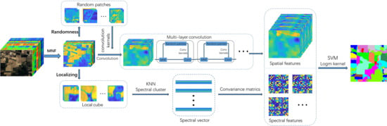
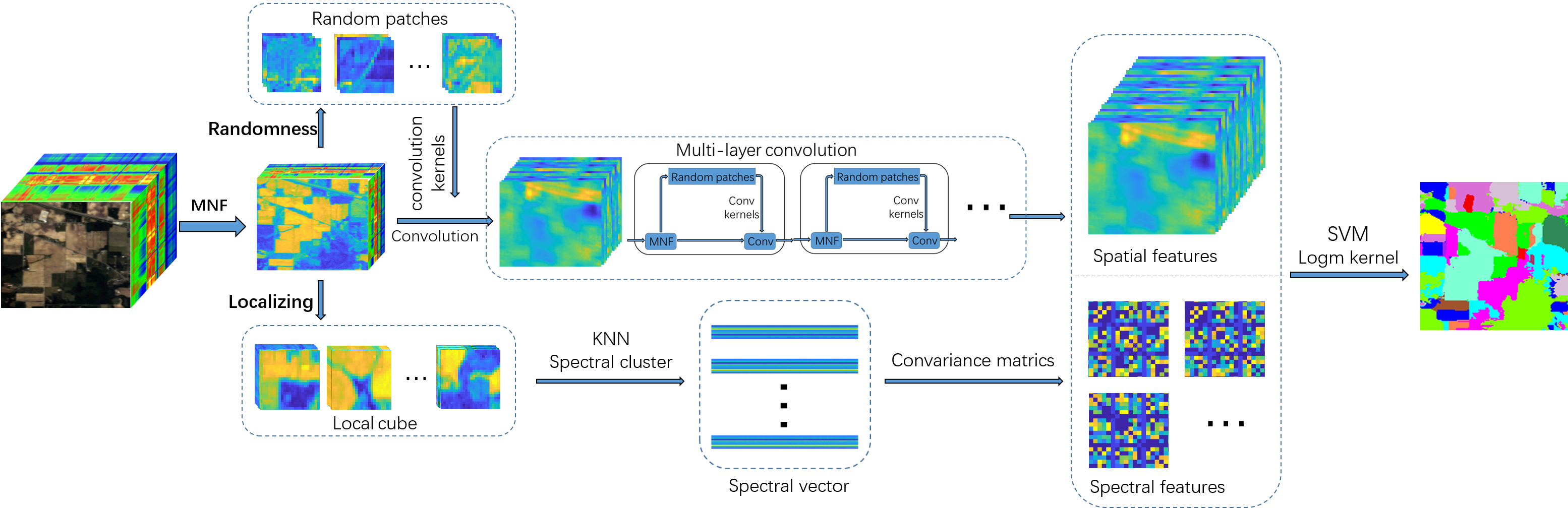
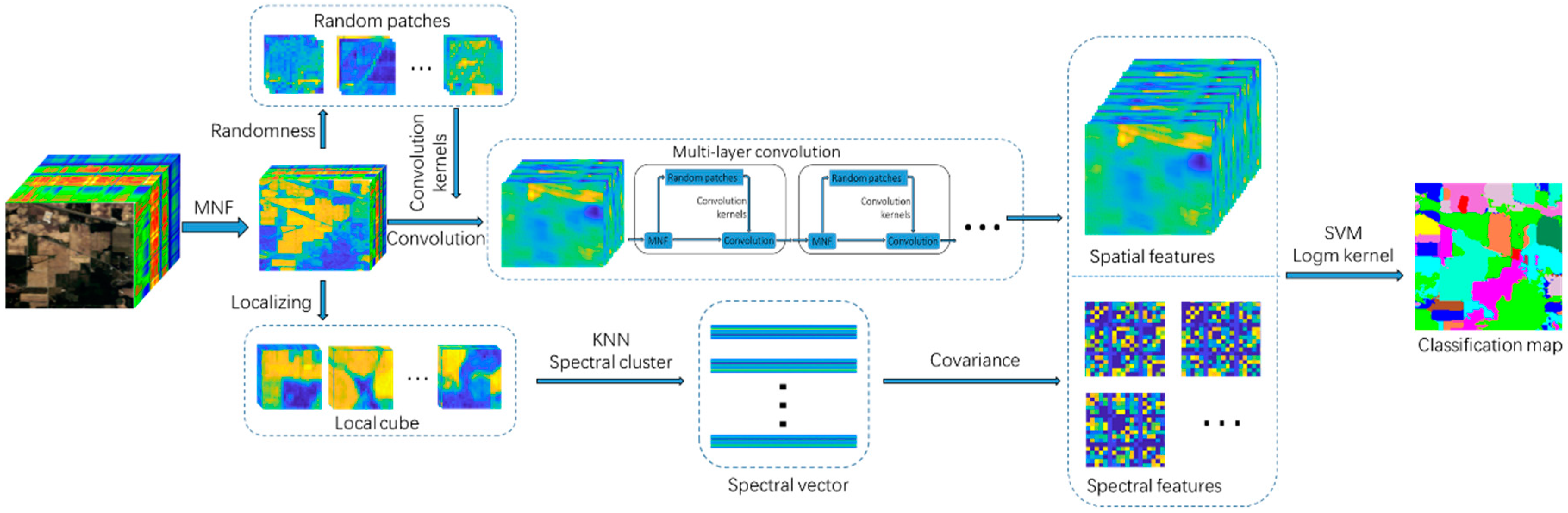
Figure 1 shows the framework of RPCC, which has two parallel branches. It obtains multi-scale convolution features via a random patches convolution [49] algorithm. Local covariance matrices are calculated to obtain all spectral correlation information for the image. Then, the obtained multi-scale spatial information and spectral covariance matrix are merged into spectral‒spatial features. Finally, we added the fused spectral–spatial features into the SVM for HSIs classification.
2.1. Maximum Noise Fraction-Based Dimensionality Reduction
Each HSI band records the sunlight in a different spectral range, and the scale between these bands are varied. So the principal components (PCs) generated by the PCA transformation calculated using the covariance matrix do not represent the characteristics of the original data well. The research of Eklundh and Singh [50] indicates that the PCs calculated using the correlation matrix consistently yielded significant improvements in SNR to comparison to those calculated using the covariance matrix. The results obtained in this study show that PCA using the correlation matrix is the desirable mode of analysis in remote sensing applications. In most remotely sensed data, the signal at any point in the image is strongly correlated with the signal at neighboring pixels, while the noise shows only weak spatial correlations. According to this, Switzer [51] developed the min/max autocorrelation factors (MAF), which in effect estimates the noise covariance matrix for salt-and-pepper noise, as well as other forms of signal degradation such as striping. In response to the inadequacy of the PCA transformation, Green et al. [21] proposed minimum noise fraction (MNF) transformation, which uses the MAF to estimate the noise covariance matrix for the more complicated cases that often exists in remotely sensed multispectral scanner data and provides an optimal ordering of images in terms of image quality. The challenge of MNF transform is to obtain the noise covariance matrix. Nielsen and Larsen [52] have given four different ways of estimating it. They all rely on the data being spatially correlated. One way is by computing the covariance of the first order differences, assuming the noise is temporally uncorrelated. This way, the MNF transform is identical to min/max autocorrelation factors transform [51,53]. Fang et al. [29] explained the results of comparative experiments on HSIs reduction using MNF, PCA, and independent component analysis, (ICA), and found that MNF offers great advantages for the calculation of spectral relationships. Therefore, in the present study we use MAF to estimate the noise covariance matrix and MNF as a HSIs preprocessing method to extract the spectral features.
We defined the input HSIs data as ∈. Here m, n, and z are the number of rows, columns, and spectral bands, respectively. Assuming that ∈ is separated into the noise and the signal , we have
The transformation matrix was obtained by maximizing the SNR of the signal covariance to the noise covariance:
where and are the covariance of the signal and the noise, respectively. The optimization problem of Equation (2) is equivalent to:
where represents the overall covariance of the HIS data, = + .
is estimated by MAF [51]. According to the Lagrange multiplier method, the optimal solution to Equation (3) is:
Then the eigenvalues were arranged from large to small, and the first corresponding eigenvalue vectors were used as a transformation matrix:
Therefore, the number of MNF principal components is and the output data after MNF transformation are :
2.2. Spatial Feature Extraction with Random Patches Convolution
For spatial feature extraction, the data were obtained by MNF transformation. Then, the data were whitened to reduce the correlation between different data bands. After the whitening operation, the data were .
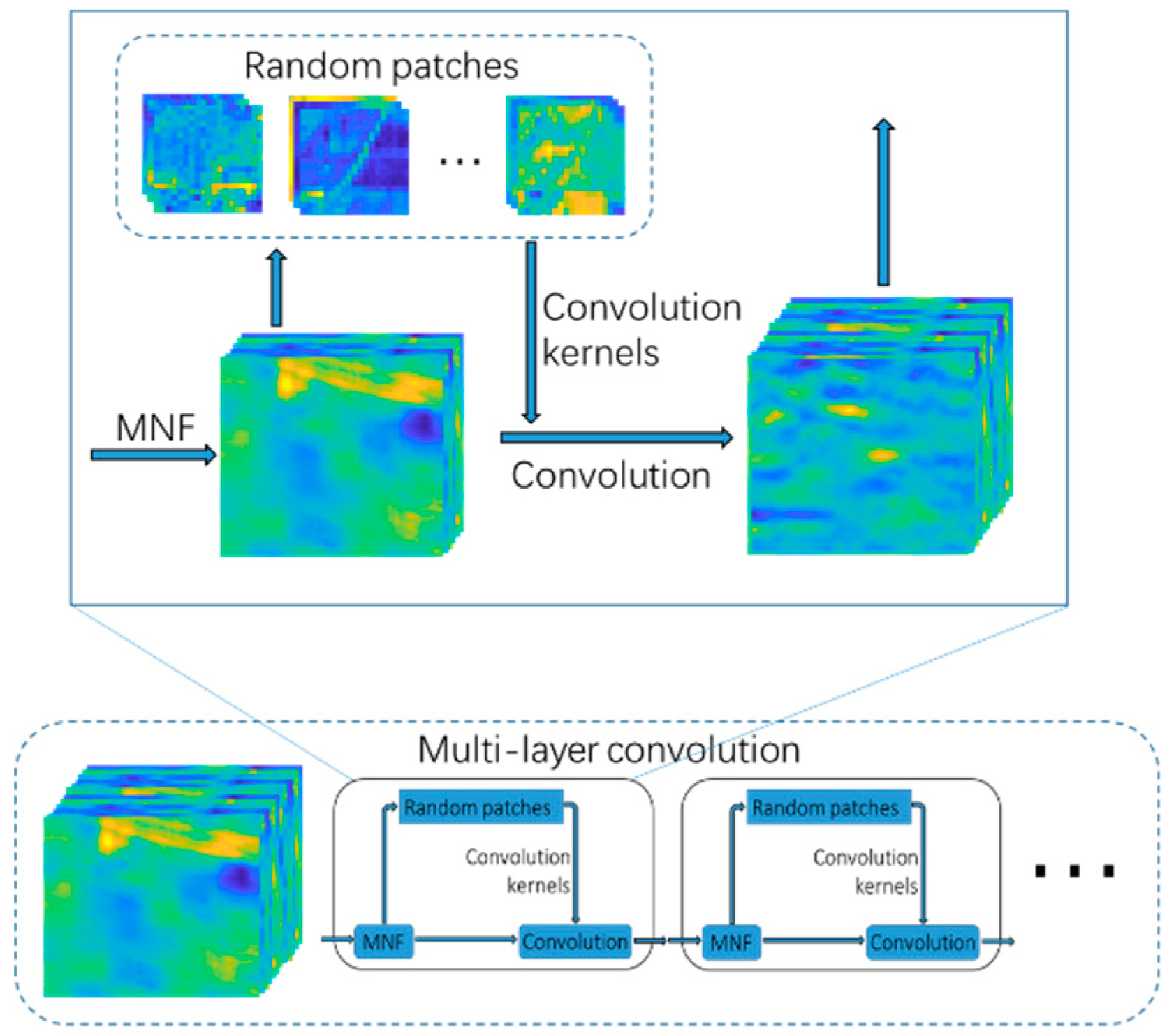
Inspired by the RPNet [49], we used multi-layer convolution, which not only has a simple architecture and requires no training but also can obtain multi-scale spatial information by extracting shallow and deep features. That can be seen in Figure 2.
We generated k random pixel locations using random functions from the data . Then we obtained k random patches by using an image window with a size of around each pixel as random patches. For the pixels at the edge of the image, the blank area is filled by mirroring the adjacent pixels. Taking a Pavia University data–set as an example, the original Pavia University data are subjected to MNF transformation (PCs = 20), a whitening processing, and 20 pixels edge mirroring to obtain data . In Section 3.2, we specifically analyzed the effect of the number of MNF PCs, the size of patches and the number of patches on the accuracy of classification.
Figure 3a is the first three-channel color composite image of with 20 randomly generated red rectangular windows; Each red window has a yellow number, from 1 to 20. Figure 3b gives the corresponding random patches extracted from . Each patch has a number corresponding to the left red window. These random patches will all be selected as convolution kernels. After obtaining the first-layer convolution feature, the above process was repeated to obtain the second layer convolution feature. The specific process is as follows.
Each random patch acts as a convolution kernel, so the random patching and whitening data convolution operations can be defined as follows:
where is the i-th feature map, , is the j-dimensional whitening data, is the convolution operator, and is the j-dimensional random patch of the i-th feature map. The stride of the 2D convolution is 1 and the vacant area is filled by mirroring the adjacent pixels.
Let and be the -th and -th layer feature sets, respectively. Then, at the beginning, the first-layer feature set . We performed MNF dimensionality reduction on the first-layer feature set to generate new random patches. Then, by convolving the with random patches, we obtained the second-layer feature set . In a similar manner, we obtained the -th-layer feature set. Finally, we obtained all the features from different layers ∈:
2.3. Spectral Feature Extraction
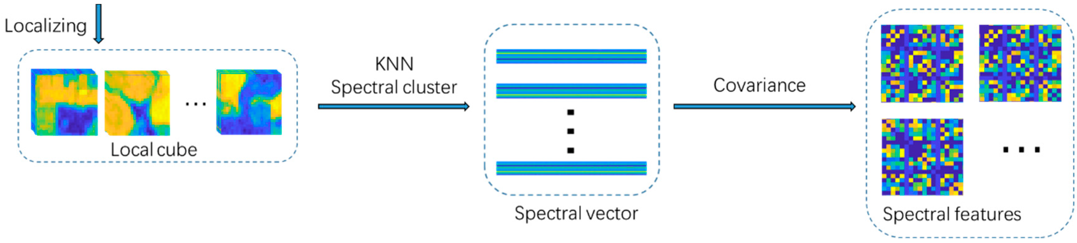
Local covariance can indicate the degree of correlation between features; [26] and [27] used local covariance for facial recognition and image classification. Fang et al. [29] used local spectral covariance for hyperspectral data classification. By comparing the spectral covariance with the entire image range, the local spectral covariance can be obtained more accurately, with more feature information and less computational complexity. As shown in Figure 4, for every pixel in the data , we obtained N local spectral cubes by using an image window with a size of . The total number of HSIs pixels is N, where . Furthermore, we used the k nearest- neighbor method to extract the spectral bands in each local spectral cube; each local spectral cube obtained the most relevant T spectral bands. is the t-th spectral band in the local cube region :
For each local spectral cube, we constructed a corresponding covariance feature matrix which is expressed as follows:
where is the mean vector of the . Finally, we obtained all of the features from all spectral cubes:
Referring to references [26,54,55], we needed to make strictly positive. Therefore, we let , where E is the unit matrix and = . It is worth noting that, since is on the Manifold space [26], the covariance matrices will be converted to Euclidean space using the method in [56]. Given two covariance matrices and , the Log-Euclidean distance (LED) was defined as follows:
where and are the F norm and the logarithm operator.
2.4. Classification Based on Spectral–Spatial Features
We transformed the spectral‒spatial features obtained by the above method to the same dimension. Let ∈ be ∈ and ∈ be ∈ by reshaped operator. Then, the spectral–spatial vectors are as follows:
It is worth noting that these features must be normalized, the formula for which is as follows:
where and are the variance, mean of and normalized spectral–spatial feature, respectively. The fused spectral–spatial are fed into the SVM classifier.
The spectral–spatial features extracted by our method combine the shallow and deep convolution features of the spatial domain, which means that the method can better characterize multi-scale feature information in hyperspectral remote sensing images. The method also combines spectral information from different local spectral cubes of the spectral domain. It can obtain spectral spatial information simply and efficiently.
Lastly, unlike the RPNet proposed by reference [49], our RPCC does not involve the fusion of raw HSI data into an SVM, and there is no nonlinear activation operation. We used the same method as in references [29,54] to approximate the matrices in the Euclidean space. The source code will be released soon (https://github.com/whuyang/RPCC).
3. Experimental Setup and Analysis
In our experiments, to overcome the categories’ imbalance problem, instead of splitting a dataset by an average percentage of each class, we specified the number of labeled samples for each annotated class of each data set. The training set is generated randomly from the ground reference data and the remaining reference samples consist of testing sets; all are listed in Table 1, Table 2 and Table 3. Then we used the LibSVM [57] implementation for the SVM classification with five-fold cross validation. The range of the regularization parameters is from to . In order to reduce the deviation caused by random sampling on classification results, all the experiments in this paper were randomly repeated 30 times using the same training and test samples number and both the average value and the standard deviation are reported. Moreover, the accuracy of each category, OA and kappa coefficient (Kappa) were chosen as criteria for quantitative assessment. All algorithms were programmed in Matlab 2017a (MathWorks, Natick, MA, USA) and tested with an Intel E5-2667v2, 128 GB and GTX1080Ti.
3.1. Data Sets
Here, we conducted experiments and evaluated our approach on three common hyperspectral public data sets.
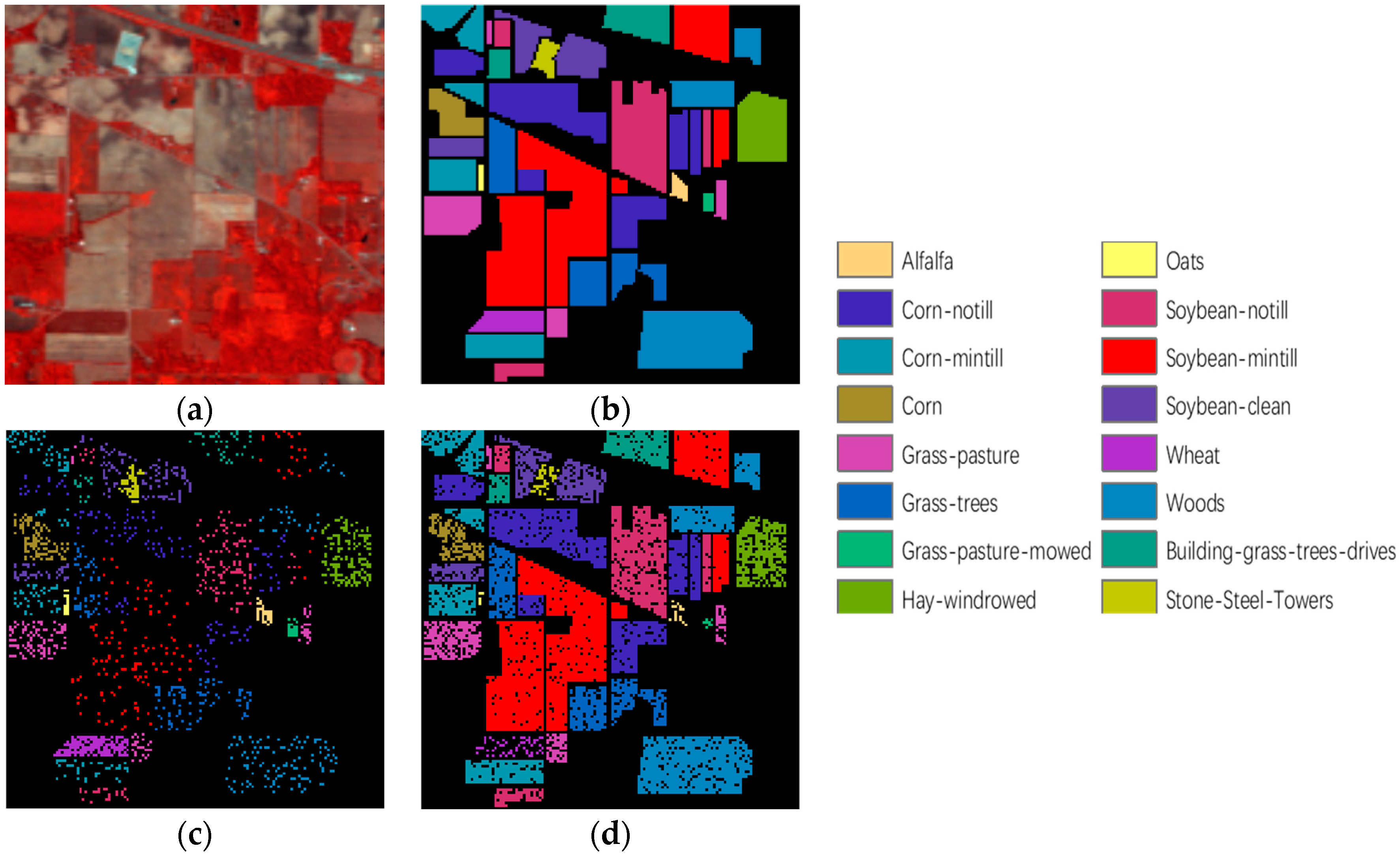
The Indian Pine HSI data‒set was used for the first experiment, as detailed in reference [58]. The data set has a rows and columns of 145 × 145 pixels and 200 spectral bands. The wavelength is from 0.4 to 2.5 μm and the spatial resolution is 20 m. The labels used for training have sixteen classes. Figure 5 gives the false color composite image (bands 36, 17, and 11 for R, G, and B, respectively) and the ground truth color map of the data set. Table 1 gives the specific training and test sample information for the experiment.
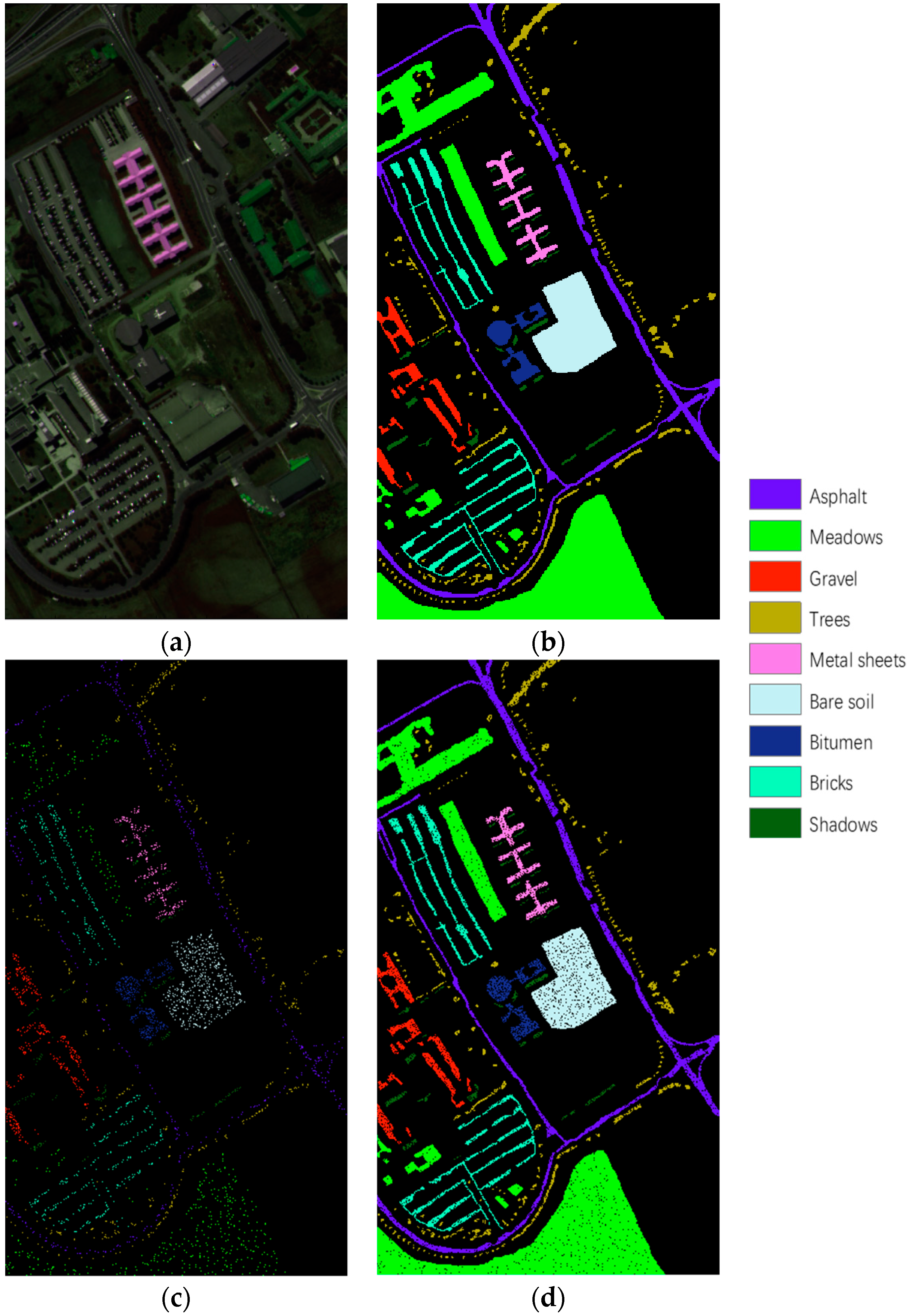
The Pavia University HSI data set was used for the second experiment, as detailed in reference [58]. The data set has a rows and columns of 610 × 340 pixels and 103 spectral bands. The wavelength is from 0.43 to 0.86 μm and the spatial resolution is 1.3 m. The labels used for training have nine classes. Figure 6 gives the false color composite image (bands 10, 27, and 46 for R, G, and B, respectively) and the ground truth color map of the data set. Table 2 gives the specific training and test sample information for the experiment.
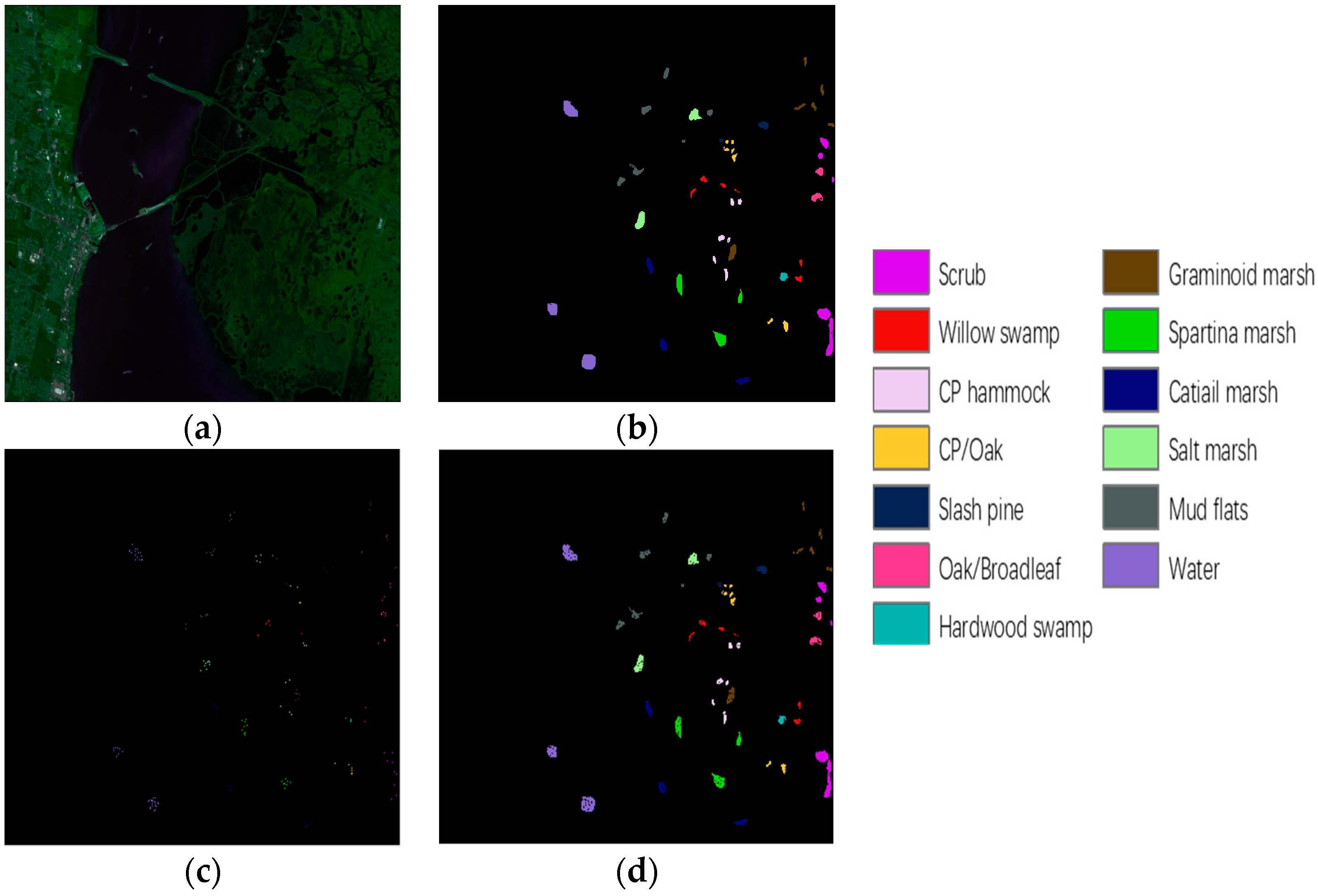
The Kennedy Space Center (KSC) HSI data set was used for the third experiment, as detailed in [58]. The data set has a rows and columns of 512 × 614 pixels and 176 spectral bands. The wavelength is from 0.4 to 2.5 μm and the spatial resolution is 1.8 m. The labels used for training have thirteen classes. Figure 7 gives the false color composite image (bands 10, 34, and 19 for R, G, and B, respectively) and the ground truth color map of the data set. Table 3 gives the specific training and test sample information for the experiment.
3.2. Parameter Analysis
There were several important parameters used in the proposed RPCC: P is the number of MNF PCs, W is the size of patches, K is the number of pixels in a local cube, N is the number of patches, and D is the number of convolutional layer. Among them, according to our algorithm design, N should be greater than or equal to P. Considering the efficiency of the algorithm, we set N equal to P.
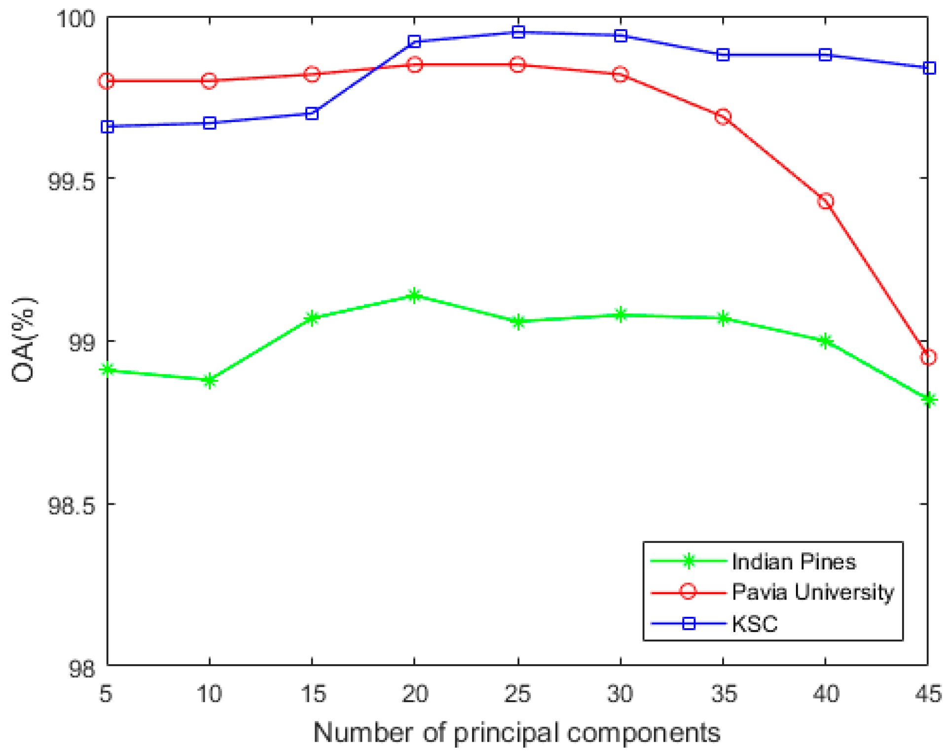
First, we designed the experiment and plotted the relationship between P and classification accuracy in our RPCC. Parameters W, K, N, and D are 25, 160, 45, and 5, respectively. As shown in Figure 8, when P increases from 5 to 20, the classification accuracy of the Indian Pine and KSC data has increased significantly, but the Pavia University rise is not obvious. When P is larger than 20, the overall accuracy (OA) of all three decreases and the OA of the Pavia University data set is significantly lower. As the P value increases, the experimental time of the three data sets is significantly longer. Considering the balance between accuracy and time consumption, we set P = 20.
Second, we analyzed the sensitivity of the classification accuracy to parameter W, with parameters P, K, N, and D set to 20, 160, 20, and 5, respectively. The value of W is 15 to 31, and the step size is 2. Figure 9 shows that as W increases from 15 to 21, the classification accuracy of the Indian Pine data set gradually increases, and the classification accuracy of KSC and University of Pavia increases slightly. When W exceeds 21, the classification accuracy of the Indian Pine data set begins to decrease, while the classification accuracy of the KSC and University of Pavia decreases slightly, and tends to be stable. So we chose W = 21.
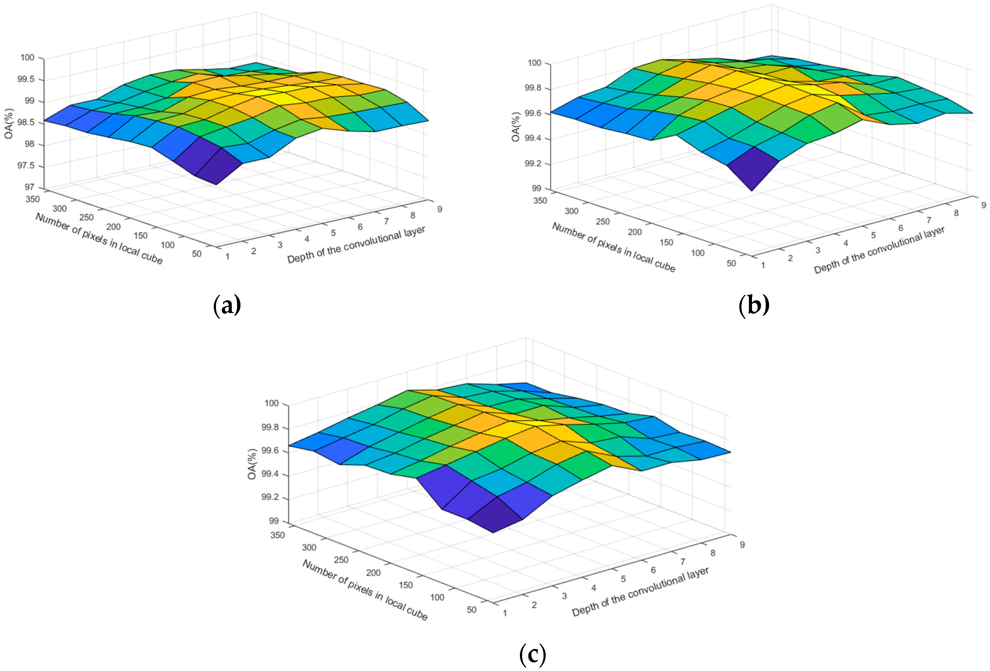
Third, we evaluated the classification accuracy of the RPCC with different values of K and D. In this experiment, K was varied from 40 to 360 with a step of 40, and D was varied from 1 to 9 with a step of 1. The parameters P, W, and N were 20, 21, and 20, respectively. Figure 10 shows that the OA for all three HSIs data sets are maintained at a high level. When K and D increase, the OA of Indian Pine, University of Pavia and KSC are gradually increasing. As can be seen in Figure 10a,c, when the highest OA of the Indian Pine and KSC data sets was achieved, K = 160 and D = 5. When the highest classification accuracy of Pavia University data-set was obtained, D = 5 and K = 160, 200, or 240. Taking into account the computational efficiency and the previous work of reference [29], we set K = 160 and D = 5. Table 4 summarizes all the parameters in our experiments.
3.3. Classification Results
Our method was compared with RAW [59], MNF [21], and the five state-of-the-art HSIs classification methods, SMLR-SpTV [60], Gabor-based [33], EMAP [35], LMRC [29], and RPNet [49], and a detailed analysis was carried out using the quantitative and qualitative experimental results. The last five methods were developed in recent years [61,62] and are closely related to our methods. SMLR-SpTV uses a spatially adaptive hidden Markov field and spectral fidelity to obtain spectral–spatial information for HSIs classification. The Gabor-based method uses the classical Gabor filter to obtain effective spectral features. EMAP can extract the geometric features of HSIs and form a feature vector space that describes the information of HSIs structure attributes, which is an effective spectral–spatial classification method. LMRC integrates spatial context information and spectral correlation information for HSIs classification by means of local covariance matrix representation. RPNet has a new multi-layer convolution structure that can quickly obtain high-precision classification results. The Monte Carlo iteration of SMLR-SpTV method is 10 times. The EMAP attribute extraction threshold is 2.5–10% according to the mean of each feature, the standard deviation attribute step is 2.5%, and the area attribute threshold is 200,500, and 1000, respectively. The parameters in the Gabor-based, LMRC, and RPNet methods are the same as the ones used in references [29,33,49]. Table 5, Table 6 and Table 7 show the results of quantitative experiments for all methods. Figure 11, Figure 12 and Figure 13 give color classification results maps of the corresponding methods.
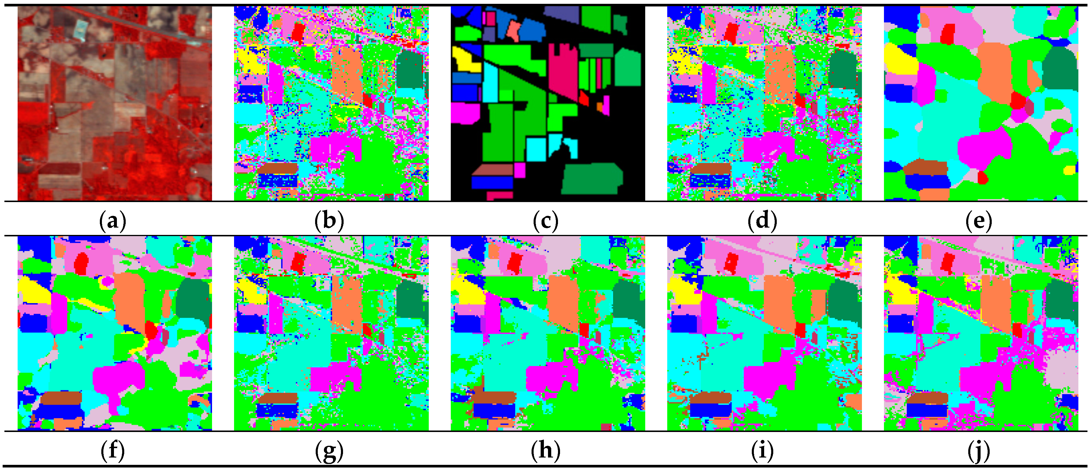
The quantitative results of the aforementioned state-of-the-art methods in the first experiment are shown in Table 5, and Figure 11 shows the corresponding classification map. It is clear that our RPCC approach achieves the highest OA and Kappa as well as the best classification map. From Table 5 it is clear that, in most categories, our RPCC has the best class accuracy. Among the 16 categories, only the accuracy of Corn, Soybean–clean, Wheat, and Buildings–Grass–Trees–Drives are lower than SMLR-SpTV and LCMR. Considering the accuracy of all the categories, our proposed RPCC achieves an advantage of 2%–22% on the indicator of OA and Kappa. The RAW and MNF methods only use spectral information, and more noise and misclassification can be seen on their classification map from Figure 11, such as for the Soybeans–min class in the middle of the map. Clearly, spatial information is beneficial for improving classification. The remaining six methods all consider spectral–spatial features. Comparing the classification map obtained using the SMLR-SpTV, Gabor-based, and EMAP methods, it can be seen that the SMLR-SpTV and Gabor-based methods produce smoother classification maps. In the integrated SMLR-SpTV method, MRF improves the classification performance and allows spatially smooth classification. The LMRC and RPNet methods both have good classification performance; however, our proposed RPCC obtains better results by combining the advantages of LMRC and RPNet. The RPCC not only uses spectral–spatial features to reduce misclassification, but also uses local k-nn clustering, covariance expression, and random patches to make the obtained spectral–spatial features more discriminative. Therefore, RPCC has a simple and efficient feature extraction strategy that can produce competitive experimental results.
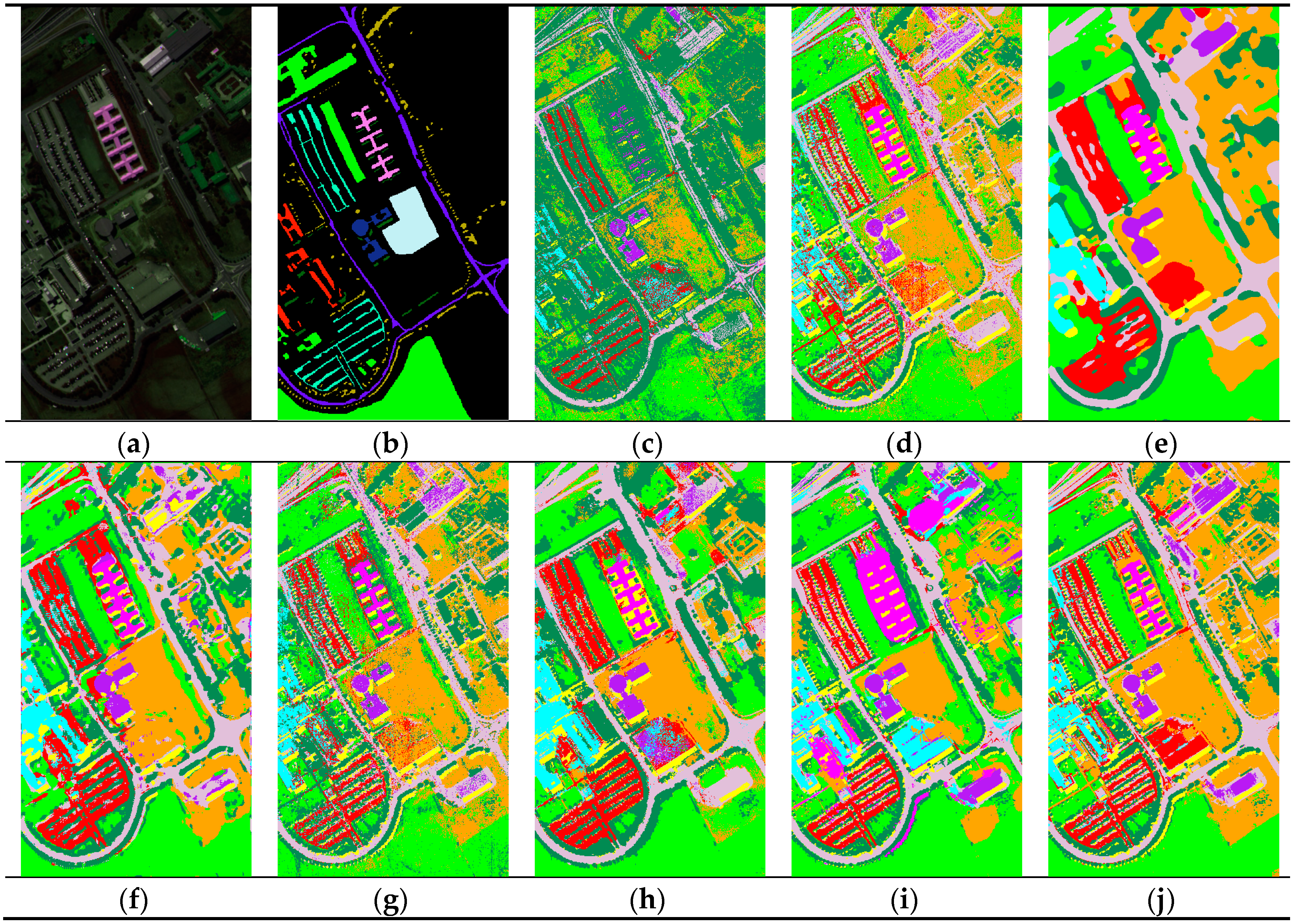
For the second experiment, Figure 12 and Table 6 show the classification results and classification accuracy, respectively, of the Pavia University data set. On the whole, five classification methods based on spectral‒spatial features have achieved similar classification accuracy. Our method still has the highest OA and Kappa. Figure 12 also illustrates that the classification maps of RAW, MNF, and EMAP are quite noisy, especially in the Bare Soil and Meadows regions. The classification maps of SMLR-SpTV and Gabor-based show overfitting. Additionally, the LCMR and RPNet methods failed to distinguish between the categories of Bricks, Bare soil, and Meadows. Therefore, our proposed RPCC method can achieve good performance in both classification mapping and accuracy.
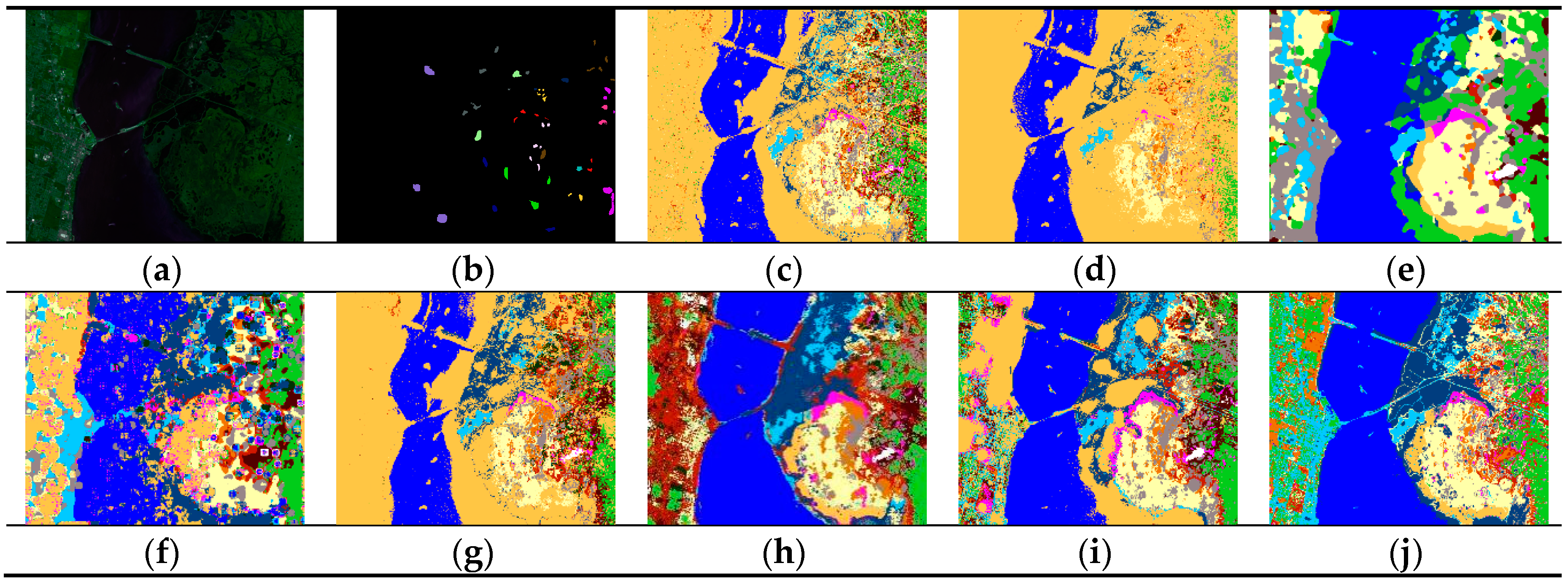
For the third experiment, Figure 13 and Table 7 show the classification results, false-color images, corresponding ground-truth maps, and classification accuracy, respectively, of the KSC data-set. Our proposed RPCC method is 1%–10% higher than the other seven methods and has the highest accuracy in all categories. Figure 13 shows that our RPCC method achieves better classification for the classes of Water, Mud flats, Salt marsh, and Cattail marsh than the other methods. Similar to the Pavia University and Indian Pine data sets, the classification maps obtained using the RAW and MNF methods show over-smoothing. The SMLR-SpTV, Gabor-based, EMAP, and RPNet methods typically misclassify Water and Cattail marsh in some areas. Moreover, the LCMR method results in a large amount of misclassification for the CP/Oak category.
4. Discussion
In Figure 11, Figure 12 and Figure 13 and Table 5, Table 6 and Table 7, a comparison with the other seven methods of the Indian Pine, Pavia University, and the KSC data-set shows that the proposed RPCC method can obtain better visual effects and higher accuracy. This proves the validity of the spectral spatial‒feature extraction pattern in our method. There are three reasons for this. First, we perform spectral clustering on each pixel neighborhood region and then calculate the spectral covariance matrix of the extracted pixels, so that we obtain spectral correlation information for all regions of the entire image. Second, the random-patch convolution can extract shallow and deep features, allowing both multi-scale and multi-layer spatial features to be combined. Third, the randomness and localization in RPCC are a kind of regularization pattern that has great potential to overcome the pepper noise and over-smoothing phenomena in HSIs processing. Through the above classification results and quantitative evaluation, our method can be a novel and effective spectral‒spatial classification framework.
In the field of machine learning, it is difficult to achieve the desired performance with single features and single models. An important method is to integrate. Typical fusion methods are early fusion and late fusion. Early fusion is a feature-level fusion that concatenates different features and puts them into a model for training. For example, these spectral-spatial classification methods in [39,40] and our RPCC are early fusion methods. Late fusion refers to the fusion of the score level. The practice is to train multiple models. Each model will have a prediction score, and the results of all models will be fused to obtain the final prediction results. Here, we have designed two late fusion methods as variants of RPCC. One is RPCC-LPR, which shares the same process as RPCC except that it uses SVM with linear, polynomial, and radial basis functions. Another is S-LPR-S-LPR, which uses SVM with linear, polynomial and radial basis functions to classify spatial and spectral features. Both methods use the majority vote method to obtain the final classification result with default parameters. Table 8 shows the classification accuracy of the three methods. It can be seen that the two simple fusion strategies do not improve the classification accuracy. On the one hand, it may be that the two methods require more complicated parameter adjustments to achieve the best results. On the other hand, since the most suitable kernel functions may be different for different features, perhaps the multiple kernel learning (MKL) method is more suitable for spectral‒spatial feature fusion. By adopting different kernels for different features, multiple kernels are formed for different parameters. Then we can train the weight of each kernel and learn the best combination of kernel functions for classification. In short, our method is very suitable as a simple baseline method based on spectral‒spatial feature classification, but there is still much room for improvement.
The computation time of the algorithm has a significant impact on various remote sensing applications. Table 9 summarizes the computational time required by the SMLR-SpTV, Gabor-based, EMAP, LCMR, RPNet, and RPCC methods. Based on the overall performance of each method in the three experiments, the SMLR-SpTV and Gabor-based methods are the slowest. This is due to the fact that the SMLR-SpTV method trained samples in 10 Monte Carlo runs and the high-dimensional features of each pixel extracted by Gabor-based methods reduce its efficiency; both of these are very time-consuming processes. The RPNet method is clearly the fastest. Compared with the CMR and EMAP methods, our proposed RPCC runs faster for two data-sets, since the efficient random convolution and simplified covariance representation operations are adopted when extracting spatial–spectral features. Our RPCC method is more time-consuming than the RPNet method for all three data sets, this is because the RPCC is subject to the construction of covariance features. This process takes up two-thirds of the total runtime of the method. Since our algorithm is a two-branch structure, spectral and spatial features can be calculated in parallel. Therefore, we can further improve the efficiency of our algorithm.
To summarize, by comparing the above algorithms on three experiments, it was shown that the RPCC method is able to extract highly discriminative features by combining both multi-scale, multi-layer convolution information and correlations between different spectral bands in the classification. The RPCC can be a competitive and robust approach for hyperspectral image classification. Specifically, our experiments show that randomness and local clustering are reliable techniques and have great potential to overcome the pepper noise and over-smoothing phenomena in HSI classification.
5. Conclusions
In this study, a new hyperspectral image classification pattern using random patch convolution and local covariance is proposed. RPCC is an effective two-branch method. First, it obtains a specified number of convolution kernels from the image space through a random strategy for extracting deep spatial features. Second, a covariance matrix is constructed between spectral bands by clustering local neighboring pixels in order to explore the correlation between different bands. Then the obtained multi-scale spatial information and spectral covariance matrix are merged into spectral‒spatial features, which are fed into an SVM classifier for HSIs classification. Experiments comparing the performance of our model with those of five closely related spectral–spatial methods showed that our RPCC method can match or exceed current state-of-the-art methods.
However, considering that the RPCC is not fast enough, we plan to design an effective and efficient spectral‒feature representation method. Furthermore, the framework of spectral–spatial feature extraction is not sufficiently coupled in our method, and we will therefore further integrate randomness and localization techniques, for example by introducing a deep spectral feature or superpixel methods.
Author Contributions
Z.F. and Y.S. conceived and designed the experiments; Y.S. performed the experiments and analyzed the data; and Y.S. wrote the paper.
Funding
This research received no external funding.
Acknowledgments
We thank the anonymous reviewers for their helpful and constructive comments and suggestions.
Conflicts of Interest
The authors declare no conflict of interest.
References
- Chang, C.-I. Hyperspectral Data Exploitation: Theory and Applications; Wiley-Interscience: Hoboken, NJ, USA, 2007. [Google Scholar]
- Kang, X.; Zhang, X.; Benediktsson, A.J. Hyperspectral anomaly detection with attribute and edge-preserving filters. IEEE Trans. Geosci. Remote Sens. 2017, 55, 5600–5611. [Google Scholar] [CrossRef]
- Wu, C.; Zhang, L.; Du, B. Kernel slow feature analysis for scene change detection. IEEE Trans. Geosci. Remote Sens. 2017, 55, 2367–2384. [Google Scholar] [CrossRef]
- Fang, L.; Li, S.; Duan, W.; Ren, J.; Benediktsson, A.J. Classification of hyperspectral images by exploiting spectral–spatial information of superpixel via multiple kernels. IEEE Trans. Geosci. Remote Sens. 2015, 53, 6663–6674. [Google Scholar] [CrossRef]
- Fang, L.Y.; Li, S.T.; Kang, X.D.; Benediktsson, A.J. Spectralspatial classification of hyperspectral images with a superpixel-based discriminative sparse model. IEEE Trans. Geosci. Remote Sens. 2015, 53, 4186–4201. [Google Scholar] [CrossRef]
- Liu, Y.; Li, J.; Du, P.; Plaza, A.; Jia, X.; Zhang, X. Class-oriented spectral partitioning for remotely sensed hyperspectral image classification. IEEE J. Sel. Top. Appl. Earth Obs. Remote Sens. 2017, 10, 691–711. [Google Scholar] [CrossRef]
- Guan, Y.; Guo, S.; Xue, Y.; Liu, J.; Zhang, X. Application of airborne hyperspectral data for precise agriculture. In Proceedings of the 2004 IEEE International Geoscience and Remote Sensing Symposium, Anchorage, AK, USA, 20–24 September 2004; pp. 4195–4198. [Google Scholar]
- Rosentreter, J.; Hagensieker, R.; Okujeni, A.; Roscher, R. Subpixel mapping of urban areas using EnMap data and multioutput support vector regression. IEEE J. Sel. Top. Appl. Earth Obs. Remote Sens. 2017, 10, 1938–1948. [Google Scholar] [CrossRef]
- Chang, H.C.; Burke, A. Integration of hyperspectral and polarimetric radar remote sensing techniques for monitoring invasive weeds. In Proceedings of the 2014 IEEE Geoscience and Remote Sensing Symposium, Quebec City, QC, Canada, 13–18 July 2014; pp. 2950–2952. [Google Scholar]
- Camps-Valls, G.; Tuia, D.; Bruzzone, L.; Benediktsson, A.J. Advances in hyperspectral image classification: Earth monitoring with statistical learning methods. IEEE Signal Process. Mag. 2014, 31, 45–54. [Google Scholar] [CrossRef]
- Hughes, G.F. On the mean accuracy of statistical pattern recognizers. IEEE Trans. Inf. Theory 1968, 14, 55–63. [Google Scholar] [CrossRef]
- Gong, M.; Zhang, M.; Yuan, Y. Unsupervised band selection based on evolutionary multiobjective optimization for hyperspectral images. IEEE Trans. Geosci. Remote Sens. 2016, 54, 544–557. [Google Scholar] [CrossRef]
- Chen, Y.; Jiang, H.; Li, C.; Jia, X.; Ghamisi, P. Deep feature extraction and classification of hyperspectral images based on convolutional neural networks. IEEE Trans. Geosci. Remote Sens. 2016, 54, 6232–6251. [Google Scholar] [CrossRef]
- Yuan, Y.; Lin, J.; Wang, Q. Hyperspectral image classification via multi-task joint sparse representation and stepwise MRF optimization. IEEE Trans. Cybern. 2016, 46, 2966–2977. [Google Scholar] [CrossRef]
- Harsanyi, J.C.; Chang, C. Hyperspectral image classification and dimensionality reduction: An orthogonal subspace projection approach. IEEE Trans. Geosci. Remote Sens. 1994, 32, 779–785. [Google Scholar] [CrossRef]
- Tan, K.; Li, E.; Du, Q. Hyperspectral image classification using band selection and morphological profiles. IEEE J. Sel. Top. Appl. Earth Obs. Remote Sens. 2014, 7, 40–48. [Google Scholar] [CrossRef]
- Chang, C.; Du, Q.; Sun, T. A joint band prioritization and band-decorrelation approach to band selection for hyperspectral image classification. IEEE Trans. Geosci. Remote Sens. 1999, 37, 2631–2641. [Google Scholar] [CrossRef] [Green Version]
- Bai, J.; Xiang, S.; Shi, L. Semisupervised pair-wise band selection for hyperspectral images. IEEE J. Sel. Top. Appl. Earth Obs. Remote Sens. 2015, 8, 2798–2813. [Google Scholar] [CrossRef]
- Yin, J.; Wang, Y.; Hu, J. A new dimensionality reduction algorithm for hyperspectral image using evolutionary strategy. IEEE Trans. Ind. Inform. 2012, 8, 935–943. [Google Scholar] [CrossRef]
- Fang, Y. Dimensionality reduction of hyperspectral images based on robust spatial information using locally linear embedding. IEEE Geosci. Remote Sens. Lett. 2014, 11, 1712–1716. [Google Scholar] [CrossRef]
- Green, A.A.; Berman, M.; Switzer, P.; Craig, M.D. A transformation for ordering multispectral data in terms of image quality with implications for noise removal. IEEE Trans. Geosci. Remote Sens. 1988, 26, 65–74. [Google Scholar] [CrossRef] [Green Version]
- Jiang, J.; Ma, J.; Chen, C.; Wang, Z.; Cai, Z.; Wang, L. SuperPCA: A Superpixelwise PCA Approach for Unsupervised Feature Extraction of Hyperspectral Imagery. IEEE Trans. Geosci. Remote Sens. 2018, 56, 4581–4593. [Google Scholar] [CrossRef] [Green Version]
- Chen, S.; Zhang, D. Semisupervised dimensionality reduction with pairwise constraints for hyperspectral image classification. IEEE Geosci. Remote Sens. Lett. 2011, 8, 369–373. [Google Scholar] [CrossRef]
- Shi, Q.; Zhang, L.; Du, B. Semisupervised discriminative locally enhanced alignment for hyperspectral image classification. IEEE Trans. Geosci. Remote Sens. 2013, 51, 4800–4815. [Google Scholar] [CrossRef]
- Chen, H.-T.; Chang, H.-W.; Liu, T.-L. Local discriminant embedding and its variants. In Proceedings of the 2005 IEEE Computer Society Conference on Computer Vision and Pattern Recognition (CVPR’05), San Diego, CA, USA, 20–25 June 2005; pp. 846–853. [Google Scholar]
- Wang, R.; Guo, H.; Davis, L.S.; Dai, Q. Covariance discriminative learning: A natural and efficient approach to image set classification. In Proceedings of the 2012 IEEE Conference on Computer Vision and Pattern Recognition, Providence, RI, USA, 16–21 June 2012; pp. 2496–2503. [Google Scholar]
- Pang, Y.; Yuan, Y.; Li, X. Gabor-based region covariance matrices for face recognition. IEEE Trans. Circuits Syst. Video Technol. 2008, 18, 989–993. [Google Scholar] [CrossRef]
- He, N.; Fang, L.; Li, S. Remote Sensing Scene Classification Using Multilayer Stacked Covariance Pooling. IEEE Trans. Geosci. Remote Sens. 2018, 56, 6899–6910. [Google Scholar] [CrossRef]
- Fang, L.; He, N.; Li, S. A New Spatial–Spectral Feature Extraction Method for Hyperspectral Images Using Local Covariance Matrix Representation. IEEE Trans. Geosci. Remote Sens. 2018, 56, 3534–3546. [Google Scholar] [CrossRef]
- Fauvel, M.; Benediktsson, J.A.; Chanussot, J. Spectral and spatial classification of hyperspectral data using SVMs and morphological profiles. IEEE Trans. Geosci. Remote Sens. 2008, 46, 3804–3814. [Google Scholar] [CrossRef]
- Pesaresi, M.; Gerhardinger, A.; Kayitakire, F. A robust built-up area presence index by anisotropic rotation-invariant textural measure. IEEE J. Sel. Top. Appl. Earth Obs. Remote Sens. 2008, 1, 180–192. [Google Scholar] [CrossRef]
- Zhu, C.; Yang, X. Study of remote sensing image texture analysis and classification using wavelet. Int. J. Remote Sens. 1998, 19, 3197–3203. [Google Scholar] [CrossRef]
- He, L.; Li, J.; Plaza, A.; Li, Y. Discriminative Low-Rank Gabor Filtering for Spectral-Spatial Hyperspectral Image Classification. IEEE Trans. Geosci. Remote Sens. 2017, 55, 1381–1395. [Google Scholar] [CrossRef]
- Benediktsson, J.A.; Palmason, J.A.; Sveinsson, J.R. Classification of hyperspectral data from urban areas based on extended morphological profiles. IEEE Trans. Geosci. Remote Sens. 2005, 43, 480–491. [Google Scholar] [CrossRef]
- Mura, M.D.; Villa, A.; Benediktsson, A.J.; Chanussot, J.; Bruzzone, L. Classification of hyperspectral images by using extended morphological attribute profiles and independent component analysis. IEEE Geosci. Remote Sens. Lett. 2011, 8, 542–546. [Google Scholar] [CrossRef]
- Gu, Y.; Liu, T.; Jia, X.; Benediktsson, A.J. Nonlinear multiple kernel learning with multiple-structure-element extended morphological profiles for hyperspectral image classification. IEEE Trans. Geosci. Remote Sens. 2016, 54, 3235–3247. [Google Scholar] [CrossRef]
- Fang, L.; He, N.; Li, S.; Ghamisi, P.; Benediktsson, A.J. Extinction profiles fusion for hyperspectral images classification. IEEE Trans. Geosci. Remote Sens. 2018, 56, 1803–1815. [Google Scholar] [CrossRef]
- Zhang, L.; Zhang, L.; Du, B. Deep learning for remote sensing data: A technical tutorial on the state of the art. IEEE Geosci. Remote Sens. Mag. 2016, 4, 22–40. [Google Scholar] [CrossRef]
- Zhang, X.; Song, Q.; Gao, Z. Spectral–Spatial Feature Learning Using Cluster-Based Group Sparse Coding for Hyperspectral Image Classification. IEEE J. Sel. Top. Appl. Earth Obs. Remote Sens. 2017, 9, 4142–4159. [Google Scholar] [CrossRef]
- Zhang, X.; Gao, Z.; Jiao, L. Multifeature Hyperspectral Image Classification with Local and Nonlocal Spatial Information via Markov Random Field in Semantic Space. IEEE Trans. Geosci. Remote Sens. 2018, 56, 1409–1424. [Google Scholar] [CrossRef]
- Zhu, L.; Chen, Y.; Ghamisi, P. Generative Adversarial Networks for Hyperspectral Image Classification. IEEE Trans. Geosci. Remote Sens. 2018, 56, 5046–5063. [Google Scholar] [CrossRef]
- Hinton, G.E.; Salakhutdinov, R.R. Reducing the dimensionality of data with neural networks. Science 2006, 5786, 504–507. [Google Scholar] [CrossRef] [PubMed]
- Bengio, Y.; Lamblin, P.; Popovici, D.; Larochelle, H. Greedy layerwise training of deep networks. Adv. Neural Inf. Process. Syst. 2007, 19, 153. [Google Scholar]
- Long, J.; Shelhamer, E.; Darrell, T. Fully convolutional networks for semantic segmentation. In Proceedings of the 2015 IEEE Conference on Computer Vision and Pattern Recognition (CVPR), Boston, MA, USA, 7–12 June 2015; pp. 3431–3440. [Google Scholar]
- Badrinarayanan, V.; Kendall, A.; Cipolla, R. SegNet: A deep convolutional encoderdecoder architecture for image segmentation. IEEE Trans. Pattern Anal. Mach. Intell. 2017, 39, 2481–2495. [Google Scholar] [CrossRef] [PubMed]
- Chen, Y.; Lin, Z.; Zhao, X.; Wang, G.; Gu, Y. Deep learning-based classification of hyperspectral data. IEEE J. Sel. Top. Appl. Earth Obs. Remote Sens. 2014, 7, 2094–2107. [Google Scholar] [CrossRef]
- Chen, X.; Xiang, S.; Liu, C.-L.; Pan, C.-H. Vehicle detection in satellite images by hybrid deep convolutional neural networks. IEEE Geosci. Remote Sens. Lett. 2014, 11, 1797–1801. [Google Scholar] [CrossRef]
- Zhao, W.; Du, S. Spectral-spatial feature extraction for hyperspectral image classification: A dimension reduction and deep learning approach. IEEE Trans. Geosci. Remote Sens. 2016, 54, 4544–4554. [Google Scholar] [CrossRef]
- Xu, Y.; Du, B.; Zhang, F. Hyperspectral image classification via a random patches network. ISPRS J. Photogramm. Remote Sens. 2018, 142, 344–357. [Google Scholar] [CrossRef]
- Eklundh, L.; Singh, A. A comparative analysis of standardised and unstandardised Principal Components Analysis in remote sensing. Int. J. Remote Sens. 1993, 14, 1359–1370. [Google Scholar] [CrossRef]
- Switzer, P. Min/max Autocor-relation Factors for Multivariate Spatial Imagery; Technical Report; Department of Statistics, Stanford University: Stanford, CA, USA, 1984; p. 16. [Google Scholar]
- Larsen, A.A.; Larsen, R. Restoration of GERIS data using the maximum noise fractions transform. In Proceedings of the First International Airborne Remote Sensing Conference and Exhibition, Strasbourg, France, 11–15 September 1994. [Google Scholar]
- Gordon, C. A generalization of the maximum noise fraction transform. IEEE Trans. Geosci. Remote Sens. 2000, 38, 608–610. [Google Scholar] [CrossRef] [Green Version]
- Huang, Z.; Wang, R.; Shan, S.; Van Gool, L.; Chen, X. Cross Euclidean-to-Riemannian metric learning with application to face recognition from video. IEEE Trans. Pattern Anal. Mach. Intell. 2017, 40, 2827–2840. [Google Scholar] [CrossRef] [PubMed]
- Wang, W.; Wang, R.; Huang, Z.; Shan, S.; Chen, X. Discriminant analysis on Riemannian manifold of Gaussian distributions for face recognition with image sets. IEEE Trans. Image Process. 2018, 27, 151–163. [Google Scholar] [CrossRef]
- Arsigny, V.; Fillard, P.; Pennec, X.; Ayache, N. Geometric means in a novel vector space structure on symmetric positive-definite matrices. SIAM J. Matrix Anal. Appl. 2006, 29, 328–347. [Google Scholar] [CrossRef]
- Chang, C.C.; Lin, C.J. LIBSVM: A library for support vector machines. ACM Trans. Intell. Syst. Technol. 2011, 2, 389–396. [Google Scholar] [CrossRef]
- Hyperspectral Remote Sensing Scenes. 2017. Available online: http://www.ehu.eus/ccwintco/index.php?title=Hyperspectral_Remote_Sensing_Scenes (accessed on 10 March 2017).
- Melgani, F.; Bruzzone, L. Classification of hyperspectral remote sensing images with support vector machines. IEEE Trans. Geosci. Remote Sens. 2004, 42, 1778–1790. [Google Scholar] [CrossRef] [Green Version]
- Sun, L.; Wu, Z.; Liu, J.; Xiao, L.; Wei, Z. Supervised Spectral-spatial Hyperspectral Image Classification with Weighted Markov Random Fields. IEEE Trans. Geosci. Remote Sens. 2015, 53, 1490–1503. [Google Scholar] [CrossRef]
- He, L.; Li, J.; Liu, C. Recent Advances on Spectral-Spatial Hyperspectral Image Classification: An Overview and New Guidelines. IEEE Trans. Geosci. Remote Sens. 2017, 56, 1579–1597. [Google Scholar] [CrossRef]
- Gao, F.; Wang, Q.; Dong, J.; Xu, Q. Spectral and Spatial Classification of Hyperspectral Images Based on Random Multi-Graphs. Remote Sens. 2018, 10, 1271. [Google Scholar] [CrossRef]
Figure 1.
The framework of our proposed random patches convolution and local covariance-based classification (RPCC).
Figure 1.
The framework of our proposed random patches convolution and local covariance-based classification (RPCC).

Figure 2.
The workflow of spatial feature extraction with random patches convolution.

Figure 3.
(a) The first three-channel color composite image of with 20 pixels edge mirroring. (b) The random patches from .
Figure 3.
(a) The first three-channel color composite image of with 20 pixels edge mirroring. (b) The random patches from .
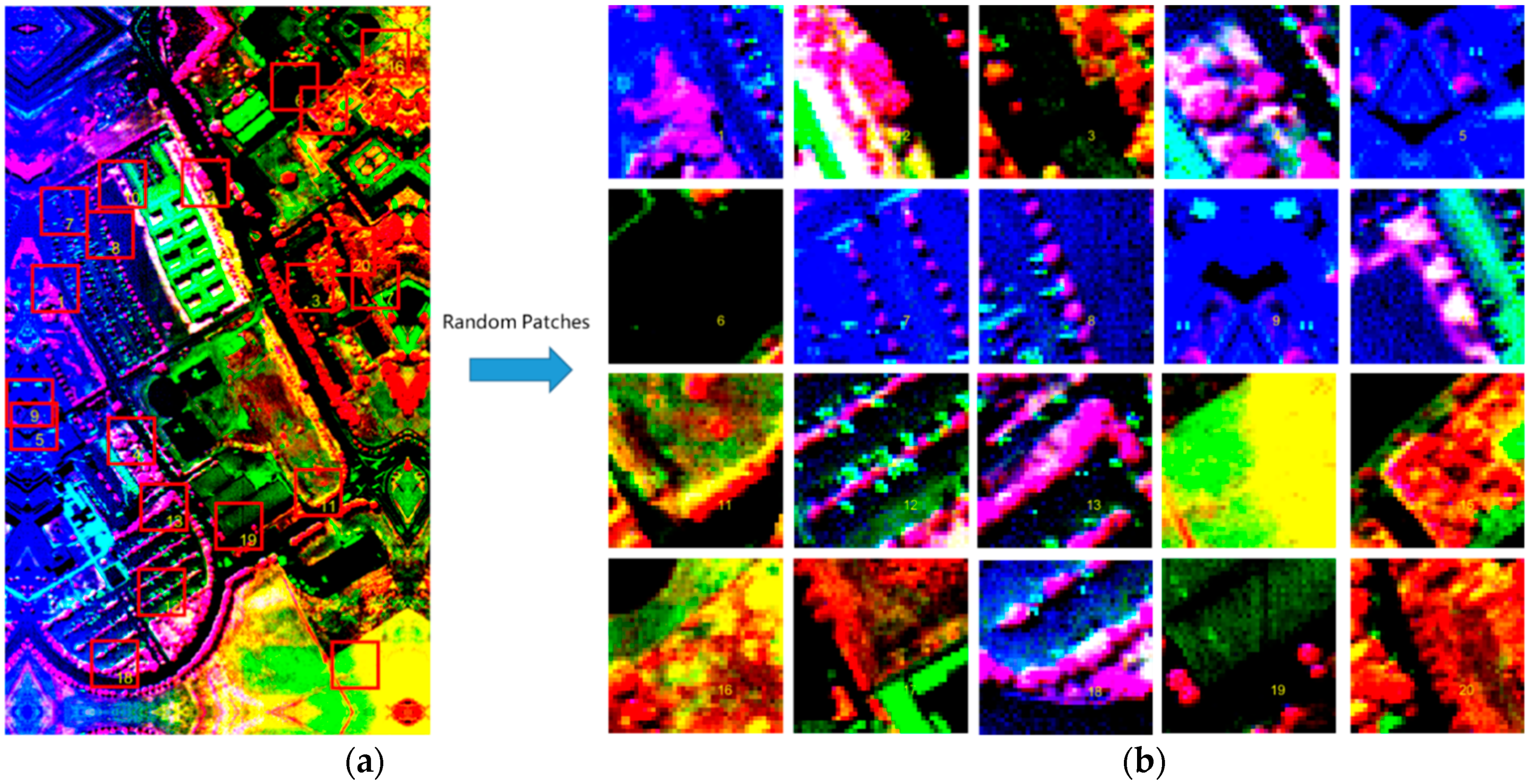
Figure 4.
The workflow of spectral feature extraction.

Figure 5.
The Indian Pine data set. (a) False color composite image; (b) ground truth color map; (c) training set; (d) test set.
Figure 5.
The Indian Pine data set. (a) False color composite image; (b) ground truth color map; (c) training set; (d) test set.

Figure 6.
The Pavia University data set. (a) False color composite image; (b) ground truth color map; (c) training set; (d) test set.
Figure 6.
The Pavia University data set. (a) False color composite image; (b) ground truth color map; (c) training set; (d) test set.

Figure 7.
The KSC data set. (a) False color composite image; (b) ground truth color map; (c) training set; (d) test set.
Figure 7.
The KSC data set. (a) False color composite image; (b) ground truth color map; (c) training set; (d) test set.

Figure 8.
Sensitivity analysis of the number of principal components and classification accuracy for three data sets. OA: Overall Accuracy, KSC: Kennedy Space Center.
Figure 8.
Sensitivity analysis of the number of principal components and classification accuracy for three data sets. OA: Overall Accuracy, KSC: Kennedy Space Center.

Figure 9.
Sensitivity analysis of the size of patches and classification accuracy for three data sets. OA: Overall Accuracy, KSC: Kennedy Space Center.
Figure 9.
Sensitivity analysis of the size of patches and classification accuracy for three data sets. OA: Overall Accuracy, KSC: Kennedy Space Center.

Figure 10.
Sensitivity analysis of the number of pixels, the number of convolutional layer and classification accuracy for three data sets. OA: Overall Accuracy, KSC: Kennedy Space Center (a) Indian Pine data set; (b) Pavia University data set; (c) KSC data set.
Figure 10.
Sensitivity analysis of the number of pixels, the number of convolutional layer and classification accuracy for three data sets. OA: Overall Accuracy, KSC: Kennedy Space Center (a) Indian Pine data set; (b) Pavia University data set; (c) KSC data set.

Figure 11.
The Indian Pine classification results. (a) False-color image; (b) ground-truth color map; (c) RAW; (d) MNF; (e) SMLR-SpTV; (f) Gabor-based; (g) EMAP; (h) LCMR; (i) RPNet; (j) proposed RPCC.
Figure 11.
The Indian Pine classification results. (a) False-color image; (b) ground-truth color map; (c) RAW; (d) MNF; (e) SMLR-SpTV; (f) Gabor-based; (g) EMAP; (h) LCMR; (i) RPNet; (j) proposed RPCC.

Figure 12.
The Pavia University classification maps. (a) False-color image; (b) ground-truth color map; (c) RAW; (d) MNF; (e) SMLR-SpTV; (f) Gabor-based; (g) EMAP; (h) LCMR; (i) RPNet; (j) proposed RPCC.
Figure 12.
The Pavia University classification maps. (a) False-color image; (b) ground-truth color map; (c) RAW; (d) MNF; (e) SMLR-SpTV; (f) Gabor-based; (g) EMAP; (h) LCMR; (i) RPNet; (j) proposed RPCC.

Figure 13.
The KSC classification maps. (a) False-color image; (b) ground-truth color map; (c) RAW; (d) MNF; (e) SMLR-SpTV; (f) Gabor-based; (g) EMAP; (h) LCMR; (i) RPNet; (j) proposed RPCC.
Figure 13.
The KSC classification maps. (a) False-color image; (b) ground-truth color map; (c) RAW; (d) MNF; (e) SMLR-SpTV; (f) Gabor-based; (g) EMAP; (h) LCMR; (i) RPNet; (j) proposed RPCC.


Table 1.
Training and test numbers for the Indian Pine HSI.
| Class | Name | Training | Test |
|---|---|---|---|
| 1 | Alfalfa | 30 | 16 |
| 2 | Corn—no till | 150 | 1278 |
| 3 | Corn—min till | 150 | 680 |
| 4 | Corn | 100 | 137 |
| 5 | Grass/pasture | 150 | 333 |
| 6 | Grass/trees | 150 | 580 |
| 7 | Grass/pasture—mowed | 20 | 8 |
| 8 | Hay/windrowed | 150 | 328 |
| 9 | Oats | 15 | 5 |
| 10 | Soybean—no till | 150 | 822 |
| 11 | Soybean—min till | 150 | 2305 |
| 12 | Soybean—clean till | 150 | 443 |
| 13 | Wheat | 150 | 55 |
| 14 | Woods | 150 | 1115 |
| 15 | Buildings/Grass/Trees/Drives | 50 | 336 |
| 16 | Stone/Steel/Towers | 50 | 43 |
| Total | 1765 | 8484 |
Table 2.
Training and test numbers for the Pavia University HSI.
| Class | Name | Training | Test |
|---|---|---|---|
| 1 | Asphalt | 548 | 6083 |
| 2 | Meadows | 540 | 18,109 |
| 3 | Gravel | 392 | 1707 |
| 4 | Trees | 542 | 2522 |
| 5 | Metal sheets | 256 | 1089 |
| 6 | Bare soil | 532 | 4497 |
| 7 | Bitumen | 375 | 955 |
| 8 | Bricks | 514 | 3168 |
| 9 | Shadows | 231 | 716 |
| Total | 3930 | 38,846 |
Table 3.
Training and test numbers for the KSC HSI.
| Class | Name | Training | Test |
|---|---|---|---|
| 1 | Scrub | 33 | 728 |
| 2 | Willow swamp | 23 | 220 |
| 3 | CP hammock | 24 | 232 |
| 4 | CP Oak | 24 | 228 |
| 5 | Slash pine | 15 | 146 |
| 6 | Oak-Broadleaf | 22 | 207 |
| 7 | Hardwood swamp | 9 | 96 |
| 8 | Graminoid marsh | 38 | 393 |
| 9 | Spartina marsh | 51 | 469 |
| 10 | Cattail marsh | 39 | 365 |
| 11 | Salt marsh | 41 | 378 |
| 12 | Mud flats | 49 | 454 |
| 13 | Water | 91 | 836 |
| Total | 459 | 4752 |
Table 4.
Parameters for the proposed random patches convolution and local covariance-based classification (RPCC) method.
Table 4.
Parameters for the proposed random patches convolution and local covariance-based classification (RPCC) method.
| Parameter | Explanation | Value |
|---|---|---|
| P | Number of MNF principal components | 20 |
| W | Size of patches | 21 |
| K | Number of pixels in local cube | 160 |
| D | Number of convolutional layer | 5 |
| N | Number of patches | 20 |
Table 5.
The classification results using different methods for Indian Pine HSI.
| Class | Table | MNF | SMLR-SpTV | Gabor-Based | EMAP | LCMR | RPNet | RPCC |
|---|---|---|---|---|---|---|---|---|
| 1 | ||||||||
| 2 | ||||||||
| 3 | ||||||||
| 4 | ||||||||
| 5 | ||||||||
| 6 | ||||||||
| 7 | ||||||||
| 8 | ||||||||
| 9 | ||||||||
| 10 | ||||||||
| 11 | ||||||||
| 12 | ||||||||
| 13 | ||||||||
| 14 | ||||||||
| 15 | ||||||||
| 16 | ||||||||
| OA | ||||||||
Table 6.
The classification results using different methods for the Pavia University HSI.
| Class | Raw | MNF | SMLR-SpTV | Gabor-Based | EMAP | LCMR | RPNet | RPCC |
|---|---|---|---|---|---|---|---|---|
| 1 | ||||||||
| 2 | ||||||||
| 3 | ||||||||
| 4 | ||||||||
| 5 | ||||||||
| 6 | ||||||||
| 7 | ||||||||
| 8 | ||||||||
| 9 | ||||||||
| OA | ||||||||
Table 7.
The classification results using different methods for the KSC HSI.
| Class | Raw | MNF | SMLR-SpTV | Gabor-based | EMAP | LCMR | RPNet | RPCC |
|---|---|---|---|---|---|---|---|---|
| 1 | ||||||||
| 2 | ||||||||
| 3 | ||||||||
| 4 | ||||||||
| 5 | ||||||||
| 6 | ||||||||
| 7 | ||||||||
| 8 | ||||||||
| 9 | ||||||||
| 10 | ||||||||
| 11 | ||||||||
| 12 | ||||||||
| 13 | ||||||||
| OA | ||||||||
Table 8.
The classification results (OA (%) and Kappa (%)) obtained by using RPCC and its two variants.
Table 8.
The classification results (OA (%) and Kappa (%)) obtained by using RPCC and its two variants.
| Data Set | RPCC | RPCC-LPR | S-LPR-S-LPR | |||
|---|---|---|---|---|---|---|
| OA | Kappa | OA | Kappa | OA | Kappa | |
| Indian Pine | ||||||
| Pavia University | ||||||
| KSC | ||||||
Table 9.
The computation time using six methods on three data sets (s).
| Data Set | SMLR-SpTV | Gabor-Based | EMAP | LCMR | RPNet | RPCC |
|---|---|---|---|---|---|---|
| Indian Pine | 213.78 | 111.49 | 30.79 | 17.11 | 17.29 | 19.97 |
| Pavia University | 1010.97 | 230.86 | 428.02 | 181.86 | 75.69 | 154.72 |
| KSC | 1737.38 | 766.94 | 179.0 | 228.4 | 35.36 | 204.67 |
© 2019 by the authors. Licensee MDPI, Basel, Switzerland. This article is an open access article distributed under the terms and conditions of the Creative Commons Attribution (CC BY) license (http://creativecommons.org/licenses/by/4.0/).
Share and Cite
MDPI and ACS Style
Sun, Y.; Fu, Z.; Fan, L. A Novel Hyperspectral Image Classification Pattern Using Random Patches Convolution and Local Covariance. Remote Sens. 2019, 11, 1954. https://0-doi-org.brum.beds.ac.uk/10.3390/rs11161954
AMA Style
Sun Y, Fu Z, Fan L. A Novel Hyperspectral Image Classification Pattern Using Random Patches Convolution and Local Covariance. Remote Sensing. 2019; 11(16):1954. https://0-doi-org.brum.beds.ac.uk/10.3390/rs11161954
Chicago/Turabian StyleSun, Yangjie, Zhongliang Fu, and Liang Fan. 2019. "A Novel Hyperspectral Image Classification Pattern Using Random Patches Convolution and Local Covariance" Remote Sensing 11, no. 16: 1954. https://0-doi-org.brum.beds.ac.uk/10.3390/rs11161954
Note that from the first issue of 2016, this journal uses article numbers instead of page numbers. See further details here.