A Method for the Destriping of an Orbita Hyperspectral Image with Adaptive Moment Matching and Unidirectional Total Variation


1
Beijing Advanced Innovation Center for Imaging Theory and Technology, Capital Normal University, Beijing 100048, China
2
College of Resource Environment and Tourism, Capital Normal University, Beijing 100048, China
3
Key Laboratory of 3D Information Acquisition and Application Ministry of Education, Capital Normal University, Beijing 100048, China
4
The School of Information Engineering, Zunyi Normal University, Zunyi 563100, China
*
Author to whom correspondence should be addressed.
Remote Sens. 2019, 11(18), 2098; https://0-doi-org.brum.beds.ac.uk/10.3390/rs11182098
Submission received: 23 July 2019
/
Revised: 23 August 2019
/
Accepted: 2 September 2019
/
Published: 9 September 2019
(This article belongs to the Section Remote Sensing Image Processing)
Abstract
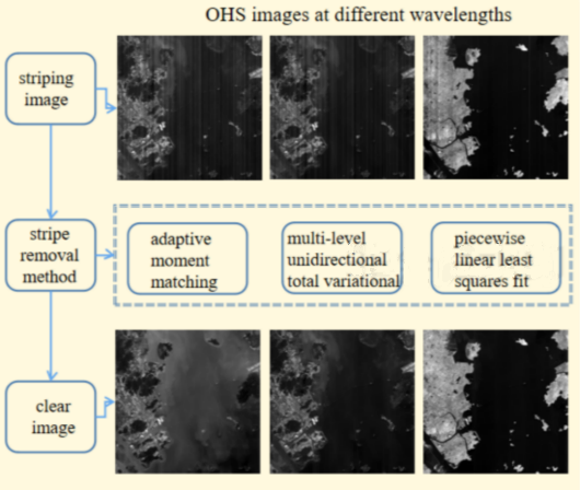
:The Orbita hyperspectral satellite (OHS) is the first hyperspectral satellite with surface coating technology for sensors in the world. It includes 32 bands from visible to near-infrared wavelengths. However, technology such as the fabricating process of complementary metal–oxide–semiconductor (CMOS) sensors makes the image contain a lot of random and unsystematic stripe noise, which is so bad that it seriously affects visual interpretation, object recognition and the application of the OHS data. Although a large number of stripe removal algorithms have been proposed, very few of them take into account the characteristics of OHS sensors and analyze the causes of OHS data noise. In this paper, we propose a destriping algorithm for OHS data. Firstly, we use both the adaptive moment matching method and multi-level unidirectional total variation method to remove stripes. Then a model based on piecewise linear least squares fitting is proposed to restore the vertical details lost in the first step. Moreover, we further utilize the spectral information of the OHS image, and extend our 2-D destriping method to the 3-D case. Results demonstrate that the proposed method provides the optimal destriping result on both qualitative and quantitative assessments. Moreover, the experimental results show that our method is superior to the existing single-band and multispectral destriping methods. Also, we further use the algorithm to the stripe noise removal of other real remote sensing images, and excellent image quality is obtained, which proves the universality of the algorithm.

1. Introduction
The orbita hyperspectral satellite (OHS) is the world's first hyperspectral satellite that uses surface coating technology for sensors, and it obtained hyperspectral images of the target object by fabricating variable filters evenly on the detector glass and then using the push-broom mode to acquire alone-track images. The wavelength of the fabricated filters is from the visible spectrum to the near-infrared spectrum. Compared with other hyperspectral satellites, OHS has the advantages of combining high spatial resolution, high spectral resolution, and the large swath width, so it breaks through the bottleneck of hyperspectral satellites, and it opens a new era of quantitative remote sensing. However, due to the influence of the CMOS sensor fabricating process, the response of the satellite sensor is non-uniform.
Compared with other real remote sensing images, the noise is more serious, which is mainly expressed as the non-periodic stripe noise. Stripes not only reduce the data interpretability and quality, but also restrict the application of the resulting images. Therefore, it is worthwhile to develop algorithms for the correction of the stripe before the succeeding image interpretation processes are performed.
In the past decades, the destriping problem has attracted many research interests. According to the data type, the stripe noise removal method can divide into two categories: Single-band image destriping methods, and multispectral image or hyperspectral image destriping methods, and according to the different method type, they can be mainly classified into four categories: The statistical-based methods, the filtering-based methods, the variation-based methods and the deep learning-based methods.
The statistical-based methods assume that the distribution of the digital number for each detector is the same, and then adjusts the target distribution to the reference one [1]. These methods mainly include moment matching [2], histogram matching [3,4] and the improved algorithms based on moment matching [5,6]. Generally speaking, these methods are the most widely utilized because of the advantages of simplicity, fast processing speed and satisfactory effect on the area where the surface is evenly covered, but the stripe removal effect is not ideal for areas covered by complex ground objects.
The filtering-based methods, such as the wavelet-based filter [7,8,9], the selective and adaptive filter [10] or the finite impulse response filter [11], etc., remove stripe noises by constructing a filter at a given frequency. These approaches are easy to achieve and can produce good results on georectified images, but for the image with non-periodic stripes, it is impossible to accurately separate the stripes and the images, resulting in a serious loss of image details. Besides, these methods introduce ringing artifacts, which damage the radiometric precision of the data when the input radiance changes abruptly.
Variational methods regard stripe removal problems as an ill-posed inverse problem and obtain destriping images by minimizing an energy function. One of the most famous variational methods is the unidirectional total variational (UTV) method [12], and this method has a good destriping effect, but it is easy to lose details at a single scale. On this basis, many improved variational models are proposed [13,14,15,16,17,18]. Liu et al. [13] proposed a 1-D variational method to estimate the statistical feature-based guidance, and the guidance information was then incorporated into 2-D optimization to control the image estimation for a reliable result. Chang et al. [14] proposed a variational destriping model that combined unidirectional total variation and framelet regularization. Hu et al. [15] proposed a MODIS stripe removal model that combined moment matching with the variational method. First, part of the stripe was removed by moment matching, and then the remaining stripe was removed by using the unidirectional total variation model. Boutemedjet et al. [16] proposed a unidirectional total variation model based on an edge-aware weighting to preserve the structure information. Moreover, some methods consider the characteristics of stripe structure or consider image decomposition to obtain clear images from striped images [19,20,21,22,23]. In [19], the proposed model employed the group sparsity to estimate the stripe component firstly, and used difference-based constraints to describe the direction information of the stripes. In [21], Chang et al. proposed a low-rank-based single-image decomposition model (LRSID) to separate the original image from the stripe component and extended the 2-D image decomposition method to the 3-D case.
The deep learning-based methods [24,25,26] use a deep convolutional neural network for correction. These methods are fast and effective after the model is built. In [24], Guan et al. proposed an innovative wavelet deep neural network from the perspective of transform and defined a special directional regularizer to separate the scene details from stripe noise.
The above methods are mainly used for single-band images without considering spectral correlation, so some methods for multispectral and hyperspectral images are proposed successively [21,27,28,29,30,31]. In [27], Adler-Golden et al. proposed an unstriped low-dimensional model using the unstriped “reference” images, which was then used to derive the destriping transform via linear regression.
In [29], Chen et al. proposed a low-rank tensor decomposition framework-based MSI destriping method by decomposing the striped image into the image component and stripe component. For the image component, the author used the spatial UTV and spectral TV regularization. Moreover, for the stripe component, the author adopted tensor Tucker decomposition and 2,1-norm regularization.
Although the above of these destriping methods have obtained a satisfactory destriping performance, they do not take into account the stripe characteristics of OHS data (we will analyze the stripe characteristics of OHS in detail in Section 2.2), and the stripes of OHS data are very obvious, non-periodic and randomly distributed. In addition, the stripes are unrelated between different bands. Some bands have very serious stripe noise, while others are weak. Based on the above characteristics of data stripes, we need to consider using some preprocessing method, such as adaptive moment matching in this paper, to reduce the noise of different bands with different noise intensity. The reduction degree of bands with severe noise is large, while that of bands with slight noise is small, which makes the stripe noise level of different bands consistent. After that, uniform parameters are used for further correction. However, the existing methods do not take this situation into account, and make the same parameter correction between different bands, so they are not applicable to OHS images. Therefore, it is necessary to propose a new stripe removal model based on the full consideration of the stripe information of OHS.
In order to realize the goal of removing stripe noises and maintaining details for the OHS image, in this paper, we propose a method based upon adaptive moment matching and multi-level unidirectional total variational to remove stripes, and a method based on piecewise linear least squares fit to restore details. Moreover, considering the spectral correlation of hyperspectral images, we extend the algorithm to a hyperspectral case. Besides, we use the split Bregman iteration method to solve the resulting minimization problem. Our approach has been tested on OHS data and compared qualitatively and quantitatively with other destriping methods. The experimental results verify the effectiveness and robustness of our approach. The main contributions of this paper are summarized as follows.
- (1)
- We discuss the OHS remote sensing image destriping method for the first time and analyze the stripe noise characteristics and cause in detail.
- (2)
- The proposed model is based on the single-band image and extended to the hyperspectral image, which makes the proposed model more robust and effective.
- (3)
- The proposed model can also be used for other real remote sensing image stripe removal, and we can get perfect results.
The remainder of this paper is organized as follows. In Section 2, OHS data and the characteristics of stripe noise are analyzed in detail. The single-band image and hyperspectral image destriping model and its optimizations are formulated in Section 3 and Section 4. We present extensive experimental results on OHS data to demonstrate the effectiveness of our method, and give a discussion in Section 5. Finally, we conclude the paper in Section 6.
2. Data
2.1. OHS Data Introduction
The Orbita hyperspectral remote sensing satellite constellation, consisting of four hyperspectral satellites and one video satellite, was successfully launched on April 26, 2018, and it realized the networking of hyperspectral satellites with a strong capability of obtaining hyperspectral data. Table 1 gives the main parameters of OHS.
2.2. OHS Image Stripe Noise Analysis
The OHS has 32 bands, and the wavelength ranges from 400 to 1,000 nm. The first 16 bands and the latter 16 bands have different expressions in the image. The first 16 bands have a small change in grayscale, which is reflected in uniform brightness in the image, while the latter 16 bands have a large change in grayscale, which is reflected by an obvious difference in light and dark in the image. Therefore we should consider this feature when removing OHS stripe noises.
Non-uniformity is widely present in CMOS sensors. When we use a uniform light source as the illumination source, the output signals from each pixel of the image sensor should be the same under perfectly ideal conditions [32]. However, due to the inherent structure of the CMOS sensors, the response between CMOS sensor units will be inconsistent, which is mainly due to the influence of the CMOS fabrication process or the doping concentration of the material, and appears as a column stripe on the image.
We chose the original image of OHS for stripe analysis. Figure 1 shows images with 5000 × 5000 pixels of different bands.
It can be observed that the stripe noise of OHS is vertically distributed along the track direction. Stripes are generally randomly appearing in multiple columns or single columns, and the stripes are so wide and dense that the real image information is lost in some bands. Also, it holds the characteristics of obviousness, non-periodicity, globality and the random distribution of light and dark stripes. Finally, there is no correlation between stripe noises of different bands, and the noise level varies greatly between different bands.
Based on the analysis of the image stripe noise, we draw the following conclusions. Firstly, stripe noise is very serious in some bands, and the destriping ability of some existing destriping methods is directly related to the degree of image detail loss. When destriping this serious noise, larger regularization parameters will be adopted, resulting in a great loss of details. So we need to consider first to suppress the image noise to a certain extent without losing the image information. Moreover, the stripe noise degree between different bands varies, so the existing method cannot remove all band stripe noise at the same time. Based on the above conclusions, we propose the algorithm in Section 3 and Section 4.
3. Single-Image Destriping Method
In this paper, we propose a stripe removal model based on the characteristics of different bands and the expressions of stripes for OHS data. Firstly, adaptive moment matching is used to deal with the stripe, and most of the stripe noises are removed while ensuring the image column mean curve. Then, based on the unidirectional total variational model and multi-level decomposition, an energy functional is constructed, which is composed of the data fidelity term, the gradient fidelity term and the regular term. The energy functional is solved by the splitting Bregman algorithm. Finally, the vertical detail is restored by piecewise linear least squares fitting.
3.1. Adaptive Moment Matching Stripe Noise Removal Model
Ideally, the traditional moment matching method defines the stripe removal model as a linear formula and adjusts the mean and standard deviation of the images formed by each sensor to a reference value, as shown in Equation (1):
where DNcal_i is the grayscale value of the corrected pixel, DNraw_i is the grayscale value of the original pixel, Bi stands for the gain of sensor i, and NGi stands for the offset of sensor i. In formula (2), δi is the standard deviation of each image column i, and δr is the reference standard deviation (In general, δr is equal to the standard deviation of the whole image). In formula (3), Meani is the mean of each image column i, and Mean is the reference mean (In general, Mean is equal to the average value of the whole image).
The traditional method of moment matching adjusts the mean and standard deviation of all columns to the mean and standard deviation of the reference column, resulting in the mean value of the image column being approximately a straight line after moment matching. This method cannot reflect the distribution of the mean of the real image column, resulting in a ladder effect and changing the actual spectral distribution of the image. Different from this method, the adaptive moment matching method in this paper does not use the mean and standard deviation of the whole image, but uses the mean and standard deviation in the moving window, which is equivalent to smoothing the original column mean curve of the image.
In addition, it is considered that the same moving window width is not entirely applicable to different bands, different stripe characteristics and different coverage areas. Therefore, we need to set the adaptive moving window size according to the gray level of the image and the land cover type.
First, we should set the maximum value Wmax, minimum value Wmin and the fixed window size W of the moving window. In general, we set Wmin to be equal to the maximum width of the stripe in the image, and then set Wmax to be equal to a quarter of the image width, and set W to be equal to half of the sum of Wmax and Wmin. However, considering the characteristics of a large difference in the grayscale of the OHS data, for example, the water of the latter 16 bands has a large difference in grayscale from other objects, then the gray value of the water is so small that the column mean variance corresponding to a large moving window is very small. In this case, the upper limit Wmax of the moving window needs to be lowered. Therefore, before setting the maximum value Wmax of the moving window, the image column mean should be calculated first, and the attribute of the region on the image should be judged according to the column mean value. According to the set threshold value ρb (b = 1, 2, ..., B, B stands for the number of bands) and the comparison with the column mean value, the attribute of the region is divided into two categories: A high-brightness region (column mean value < ρb) and a low-brightness region (column mean value > ρb).
For the former, we use a larger Wmax. Otherwise, we use a smaller Wmax. On the basis of the (Wmin, Wmax, W) corresponding to the two types of data, we obtain the minimum variance DWmax_min corresponding to each Wmax, the maximum variance DWmin_max corresponding to the each Wmin, and the variance value (DW_min, DW_max) corresponding to each W width.
Therefore, the upper and lower limits (Dmin, Dmax) of the variance corresponding to the two types of moving window ranges are:
Then, according to the mean of the image column, the region and the corresponding (Dmin, Dmax) are determined, and by calculating the variance D of the mean value of the image column in the window W, we can obtain the image information in the window:
If D is large, indicating that the amount of image information in the window is large, the width W of the moving window is decreased; otherwise, W is increased. Loop this operation until the value D is within the defined range (Dmin, Dmax).
Finally, the weighted average of the mean Mean and the standard deviation δr of each column data in the moving window is obtained, and the gain Bi and offset NGi are obtained according to formula (2) and (3).
After the above steps, we can get the image IadaptMM, B and NG (Let B and NG be the matrices where the gain and offset are expanded along the column direction to the number of image rows) after the adaptive moment matching correction.
The OHS image can be processed by this method to remove the stripe noise in the general scene. However, for some complex scenes, the adaptive moving window moment matching method cannot completely remove the stripe noise, but serious stripe noise will be reduced and image details will not be lost, which will improve the accuracy of later model optimization.
3.2. Multi-Level Unidirectional Total Variation Stripe Noise Removal Model
A remote sensing image with stripes can be expressed by a mathematical formula as follows:
where r = 1, 2, ..., R, c = 1, 2, ..., C. R and C stand for the number of the rows and columns respectively. Here Is represents the original image, and u represents the corrected image, and s represents the stripe noise in the image. Obviously, the stripe in the remote sensing image can be regarded as an additive structural noise, and the gradient change is mainly concentrated in the x-axis (let the direction perpendicular to the stripe be the x-axis), while the change in the y-axis (let the direction along the stripe be the y-axis) is much smaller than the x-axis. Figure 2 shows the gradient of the x-axis and y-axis.
In this paper, we use this stripe feature to obtain the optimal solution of the model by minimizing the energy functional. The energy functional of the variational model is proposed as follows:
where the operators Dx, Dy denote the first-order forward finite difference operators along the x-axis (horizontal direction) and y-axis (vertical direction). The first term of the energy functional variation model is the data fidelity term, which is to make the corrected image as close as possible to the image after adapted moment matching, and the second term is the gradient fidelity term to ensure the gradient information along the track direction. The third term is the regularization term, which is designed to maximize stripe removal. λ1, λ2 is the regularization parameter, which is used to adjust the proportion between the fidelity and the regularization term.
Since the functional model contains a non-differentiable and inseparable L1 norm, this paper uses the split Bregman iterative algorithm to solve the problem.
First, for the problem (7), two auxiliary variables are introduced, and the unconstrained minimization problem is turned into the constrained minimization problem, that is, we can rewrite Equation (7) as Equation (8).
where α, β is a positive penalty parameter. The Bregman variables introduced by blx and bly are used to accelerate the iterative process. In this way, the minimization problem can be decomposed into three sub-problems of u, dlx and dly.
Sub-problems about u:
This equation is a least squares problem, which is equivalent to the following equation:
The above problem can be solved by a fast Fourier transform.
Sub-question about dlx:
Equation (11) can be solved by the soft-shrinkage operator, and the following equation can be obtained:
where
Sub-question about dly:
Equation (14) can be solved by the soft-shrinkage operator, and the following equation can be obtained:
Finally, update the Bregman variable blx, bly as follows.
However, only using the parameter λ does not completely guarantee the details, which will result in a loss of data. Therefore, the multi-level iterative method is used to improve. First, the image after adapted moment matching f is used as the source image for (8)–(16) correction, and the difference between the source image f and the corrected result u1 is taken as the source image of the second iteration. After multiple iterations, all the results are summed as the corrected image usum.
Among them, in each iteration, λ2 should decrease as the number of iterations increases. In general, the first iteration is to remove most of the stripes, and the latter iteration is to restore the image details.
3.3. Piecewise Linear Least Squares Fitting for Restoring Details
Most of the image details can be restored during multi-level iterations, but some linear structures are very similar to stripes, and they cannot be wholly recovered by relying on multi-level iterations, and the number of iterations has a significant impact on processing efficiency. Therefore, we use piecewise linear least squares fitting to restore linear details. We first divide the data (IadaptMM and usum) into M segments along the track direction, and we can get the data (0 < m < M) and the data um (0 < m < M), and then perform linear fitting between each column data of and each column data of um, finally to obtain the optimal parameters km,j and bm,j of each segment of data.
The linear model (17) was constructed and the km,j and bm,j was solved by using the Equation (18):
where j is the column number and m is segment number.
Finally, we use km,j and bm,j to solve the image after linear fitting. After getting Ipoly, we calculate the middle value of Ipoly, IadaptMM and usum:
Compare Imedian and usum according to the set threshold t1, t2, and a certain range beyond the threshold value is regarded as image details, and the final Iout is the following formula (21).
In summary, our destriping steps are shown in Algorithm 1.
| Algorithm 1 |
| Input: Image Is contaminated by stripes, the parameters ρb, Wmin, Wmax, W, λ1, λ2, α, β, out-iter, in-iter, t1, t2 1: Substitute Is into Equations (1) to (5). 2: Initialize u0 = IadpatMM, dlx = dly = blx = bly = 0 3: for n = 1: out-iter do if (n = 1) then f = IadpatMM, usum = 0 else f = IadpatMM − un end if for m = 1: in-iter do Compute unm+1 by solving (9). Update dlx and dly by (11) and (14), respectively. Update the Bregman variable blx, bly by (16). end for Update usum by usum + = un end for 4: Substitute IadaptMM and usum into Equations (17) to (20) to get Imedian, and Imedian and usum into Equation (21) to get the image Iout. Output: Iout |
4. Hyperspectral Image Destriping Method
For hyperspectral images, spectral correlation is an important prior knowledge, which can provide extra image information. Moreover, processing each band of image one by one will lose the consistency between consecutive bands. Therefore, we should take into account the spectral characteristics and extend the proposed method to the 3D-case.
4.1. Adaptive Moment Matching Stripe Noise Removal Model
We adopt an adaptive moment matching model to remove stripe noise for each band of the hyperspectral image and we can see Section 3.1 for details.
4.2. Multi-Level Unidirectional Total Variation Stripe Noise Removal Model
For hyperspectral images, the model (6) can be extended to the following model:
where b = 1, 2, ..., B, and B is the number of image bands.
Considering the smooth constraints of spectral dimensions, we can extend the UTV model in (7) to define the spectral-spatial UTV model as follows:
where the Dz represents the first-order forward finite-difference operators along z-axis (spectral direction), and other parameters are the same as the model (7). The difference between (7) and (23) is the extra spectral smoothness along the z-axis.
For the formula (23), three auxiliary variables are introduced, and then the problem (23) can be transformed into (24).
where the parameter definition is the same as Equation (8). The minimization problem can be decomposed into four sub-problems of u, dlx, dly and dlz.
Sub-problems about u:
This equation is a least squares problem, which is equivalent to the following equation:
The above problem can be solved by n-D FFT.
Sub-question about dlx and dly:
The problem is the same as in Section 3.2.
Sub-question about dlz:
Equation (27) can be solved by the soft-shrinkage operator.
Finally, update the Bregman variable blx, bly, blz as follows.
Finally, we use the multi-level iterative method proposed in Section 3.2 to optimize model.
4.3. Piecewise Linear Least Squares Fitting for Restoring Details
See Section 3.3 for details.
5. Experiment Results and Discussion
In order to verify the effectiveness of the algorithm in this paper, an image of Zhuhai, China was selected for the stripe removal experiment. The experiment consists of three parts: The comparison of single-band destriping methods based on the same paradigm, the comparison of single-band destriping methods based on the different paradigm, and the comparison of hyperspectral destriping methods. Firstly, we compare our method with five other methods based upon the same paradigm: Moment matching (MM) [2], adaptive moment matching (AdaptMM) [6], unidirectional total variational (UTV) [12], multilevel unidirectional total variational (MUTV) and unidirectional total variational based moment matching (MMUTV) [15]. Then we compare our method with four recent state-of-the-art methods based on the different paradigm: adaptive wavelet-Fourier transform (WFAF), the group sparsity based regularization model (GSTV) [19], low-rank-based single-image decomposition model (LRSID) [21] and Statistical linear destriping model (SLD) [23],. Finally we compare our method with three hyperspectral destriping methods: The anisotropic spectral-spatial TV model (ASSTV) [28], the image decomposition based band-by-band low-rank regularization and spatial-spectral TV model (LRMID) [21] and lastly the low-rank tensor decomposition model (LRTD) [29].
In the following experiments, the parameters in compared methods are manually tuned according to the rules recommended by their papers to get the possibly good performance. For the parameters of our method, we would like to show the detailed discussion in Section 5.4.1.
By using the above method, stripe noise removal experiments were performed on an OHS image, and their effects were evaluated by subjective and objective evaluation criteria. The subjective evaluation criteria mainly included: Visual effects of images, spatial mean cross-track profiles (mean curve of image columns), etc., objective evaluation criteria include: Radiation quality enhancement factor (IF) [32], information entropy (H), the inverse coefficient of variation (ICV) [33], image mean (Mean), the mean relative deviation (MRD) [28,34], noise reduction (NR) and image distortion (ID) [4,11,35].
5.1. The Comparison of Single-Band Destriping Methods Based on the Same Paradigm
We extracted a sub-image of size 5000 × 5000 × 32 in our experiment and selected several bands (band 10, band 24, band 31) to display effects, and compared the experimental results with the destriping methods based on the same paradigm.
5.1.1. Subjective Evaluation of Data Quality
Figure 3, Figure 4, Figure 5, Figure 6, Figure 7, Figure 8, Figure 9, Figure 10 and Figure 11 are showing the single-band processing effect, the image detail effect, the false color image and mean cross-track profiles of each method.
The interference of the stripe noise causes the mean distribution of the original image to exhibit sharp fluctuations. According to Figure 3, Figure 4, Figure 5, Figure 6, Figure 7, Figure 8, Figure 9, Figure 10 and Figure 11, it can be seen that:
(1) Only use moment matching method has the worst correction effect [see Figure 3b, Figure 4b and Figure 5b], and the corrected column mean curve is in a straight line [see Figure 9a, Figure 10a and Figure 11a], which is inconsistent with the real image, the ladder effect is obvious after correction, but the image detail is not lost [see Figure 6b, Figure 7b and Figure 8b].
(2) There are only a few stripes in the image after the adaptive moment matching [see Figure 3c, Figure 4c and Figure 5c], the mean curve of the column is completely consistent with the original one [see Figure 9b, Figure 10b and Figure 11b], and the image details is not lost [see Figure 6c, Figure 7c and Figure 8c].
(3) The UTV method can completely remove the stripes [see Figure 3d, Figure 4d and Figure 5d], but the column mean curve changes too much [see Figure 9c, Figure 10c and Figure 11c], and this method causes the image to be too smooth, and the image detail loss is serious, especially for the vertical details [see Figure 6d, Figure 7d and Figure 8d].
(4) The MUTV method can completely remove the stripes [see Figure 3e, Figure 4e and Figure 5e], and the column mean curves are basically normal [see Figure 9d, Figure 10d and Figure 11d], but the image vertical details are lost. [see Figure 6e, Figure 7e and Figure 8e].
(5) Due to the influence of the moment matching method, the images processed by MMUTV have poor effects [see Figure 3f, Figure 4f and Figure 5f] and a lot of details are lost [see Figure 6f, Figure 7f and Figure 8f].
(6) Our method column mean curve is consistent with the original image [see Figure 9f, Figure 10f and Figure 11f] and the stripe noise is completely removed [see Figure 3g, Figure 4g and Figure 5g], and the image details are not lost [see Figure 6g, Figure 7g and Figure 8g].
Figure 12 shows the effect of the false color synthesis of the 28th, 14th and 7th bands.
According to Figure 12, the image corrected by the moment matching [see Figure 12b] or UTV [see Figure 12d] or MMUTV [see Figure 12f] method has large color distortion, and the tone cannot be consistent with the original image. Among them, the tone of the moment matching method is completely changed, and the urban area is darker than the original image, but the water is lighter than the original image. UTV is lighter in color than the original. But the color of the adaptive moment matching [see Figure 12c], MUTV [see Figure 12e] and our method [see Figure 12g] are consistent with the original image.
5.1.2. Objective Evaluation of Data Quality
In the objective evaluation standard, the radiation quality improvement factor IF is defined as the change of the gray level of the two images alone the stripe direction before and after the removal of the stripes. The calculation formula is as follows:
where mIR(i), mIE(i) represent the average of the ith column before and after the removal of the stripes, respectively. The larger the value of IF, the stronger the destriping capability of the algorithm.
Information entropy H is a reflection of the amount of image information and an important indicator for measuring the richness of the image information. The larger the information entropy of the single-band image, the richer the amount of information. The calculation formula of image information entropy H(x) is:
where bit is the maximum gray value of the color depth, and p(i) is the probability density of the gray value i.
ICV is defined as the ratio of the mean to the standard deviation on an approximately isotropic region.
ICV was calculated by selecting two uniform regions, where Rm and Rs represent the mean and standard deviation of the selected image region. The larger the ICV, the better the stripe removal effect.
MRD calculates the change of a no stripe region, and thus measures the ability to retain the original healthy information. The smaller the MRD, the stronger the ability to retain the original image information.
where y(i,j) and x(i,j) are the pixel values in the destriped and raw images. M, N are row and column numbers.
NR is the noise reduction ratio achieved by the destriped method and ID is the degree of image distortion [11]. We assume:
where ui is the frequency component produced by stripes, and uj is the frequency component caused by the raw image without stripes. N stands for the total power of stripes noise in the mean power spectrum, and S stands for the total power of clear image in the mean power spectrum.
where N0 and N1 stand for the value of N in original image and destriped image, and S0 and S1 stand for the value of S in an original image and a destriped image.
Ideally, NR-> +∞ and ID ->1.
Due to the poor effect of moment matching and MMUTV, the objective evaluation index is not calculated. Table 2 is the objective evaluation of results.
Based upon the subjective quantitative evaluation criteria, compared with other algorithms based on the same paradigm, our algorithm can achieve the best balance of information retention and stripe removal.
5.2. The Comparison of Single-Band Destriping Methods Based on the Different Paradigm
We extracted a sub-image of size 800 × 800 × 32 in our experiment and chose several bands (band 3, band 15 and band 22) to display effects, and compared the experimental results with the destriping methods based on the different paradigm.
5.2.1. Subjective Evaluation of Data Quality
Figure 13, Figure 14 and Figure 15 are showing the single-band processing effect, and we further test the performance of the proposed method by a qualitative assessment: The mean cross-track profile.
From the results, we have the following observations. First, GSTV [19], LRSID [21] and our method can efficiently remove the stripe noise while WFAF and SLD [23] cannot. We can observe a lot of residual noise in Figure 13, Figure 14 and Figure 15. In addition, all of the methods can maintain the mean cross-track profiles well [see Figure 16, Figure 17 and Figure 18]. Second, LRSID can remove the stripes, but they smooth the details seriously [see Figure 15d], and the image produces some strange horizontal stripe artifacts [see Figure 13d]. Third, GSTV can eliminate most of the stripe noise, but there is still some blurry stripe when the noise is serious [see Figure 14e]. Moreover, GSTV blurs the image, causing a loss of detail [see Figure 15e]. Last, compared to other methods, our method achieves the best destriping results, removing all of the stripes while retaining most of the details in the image.
5.2.2. Objective Evaluation of Data Quality
In Table 3, we calculate the quantitative indices to show the performance of the destriping results of the methods based on the different paradigm. As shown in this table, compared with other methods, although the indicators of our method are not all the best, they are relatively satisfactory. First, the NR of WFAF and SLD are relatively low, indicating that these methods cannot completely remove noise. Second, compared with other methods, the NR of our LRSID method is very large, while the ID is relatively small, which indicates that LRSID has a blurring effect on the original image. Third, all evaluation indices of GSTV are slightly worse than our method.
5.3. The Comparison of Hyperspectral Destriping Methods
In this part, the hyperspectral images removal experiments are performed and compared with other methods. We extract a sub-image of size 800 × 800 × 32 in our experiment. The visual comparison shows in Figure 19, Figure 20, Figure 21, Figure 22 and Figure 23.
From Figure 19, Figure 20, Figure 21, Figure 22 and Figure 23 we can observe that ASSTV, LRMID and LRTD cannot remove all bands of stripe noise completely. When the noise level of different bands varies greatly, ASSTV, LRMID and LRTD cannot take into account the situation of all bands, so that it cannot remove all of the stripe noise or cause the loss of image details. For example, when we use LRMID to remove stripe noise, because the noise of some bands [Figure 19b,C] is very serious, when regularization parameters are adjusted to completely remove the noise of these bands, new horizontal stripe noise will be generated in other bands [Figure 21a,f,g]. But when we adjust the regularization parameters so that these bands can remove the stripe noise without producing artifacts, some bands with serious noise cannot completely remove the noise [Figure 21b𠄽d]. However, our method firstly weakens the image stripe noise adaptively, which can take into account the different noise levels of all bands, so we obtain satisfactory results [Figure 23].
5.4. Discussion
5.4.1. Parameter Settings
The parameters in the model are set according to the experiment result, and the weight coefficients of each energy term are adjusted appropriately according to the application requirements. Experimental results show that the parameters of the model in this paper are set as follows: In the adaptive moment matching algorithm, pb = the mean gray value of water area for each band, and when the column belongs to a high-brightness region, Wmax = cols / 3, otherwise, Wmax = cols / 4. In the variational algorithm, λ1 = 10, λ2 = 1, λ3 = 0.1, α = 1000, β = 100, γ = 10, and the maximum iteration number of multi-level decomposition = 10, and the maximum iteration number of internal unidirectional total variational = 20, and the termination condition of the iteration is ||uk+1-uk||2/||uk||2 < 1 × 10⁻⁴. In the piecewise linear least squares model, we set t1 = 10, t2 = 20 when the color depth is 10-bit.
When we conduct destriping experiments on other satellite images, we need to make the following adjustments. Firstly, we do not need to modify parameters for the adaptive moment matching method. Secondly, in the variational model, if the stripe noise is more serious, we need to increase the λ2 parameter, and vice versa. Finally, in the piecewise linear least squares model, we need to adjust parameters according to the color depth of the satellite image. For example, if the image color depth is 8, set t1 = 3 and t2 = 5.
5.4.2. Spectral Analysis
In this part, we further prove that our method can effectively preserve important spectral information before and after correction. Figure 24 and Figure 25 show the comparison of the spectral curves of water and vegetation with the methods based on the same paradigm.
According to the water and vegetation spectral curves, the moment matching [see Figure 24a and Figure 25a] and MMUTV [see Figure 24e and Figure 25e] have a large change of the water and vegetation spectral curves. The UTV method [see Figure 15c and Figure 24c] affects the peaks of some bands, and the corrected vegetation spectral curve was lower than the original one. Other methods can better maintain the original spectral curve. The peaks and troughs of the waves are consistent with the original ones.
Figure 26 shows the comparison of the spectral curves of water with methods based on the different paradigm. The spectral curves of all methods are basically consistent with the original spectral curves. However, WFAF has a smoothing effect, and some of its peaks are weakened.
Figure 27 shows the comparison of the spectral curves of vegetation of hyperspectral images. Since the method of hyperspectral stripe noise removal comprehensively considers the spectral correlation, the corrected spectral curve is not completely consistent with the original curve. Among them, LRTD makes the spectral curve too smooth, thus damaging its spectral information, and destroying the correlation between the first 15 bands. LRSID well maintains spectral correlation, but it cannot completely remove noise. Since our corrected curve is the same as the original curve, the spectral information of all bands is well preserved. Although the spectral information of some bands deviates from the original one, most of the spectral information is also preserved.
5.4.3. Running Time
All of the algorithms in the paper are tested in the desktop of a 16 GB RAM, Intel (R) Xeon(R) CPU e3-1226 v3, @3.30 GHz, the single-band test data of the running time is 1.22 MB, and the hyperspectral test data of the running time is 39.0 MB. In order to measure the efficiency of our method, we compare the running time with other comparison methods in Table 4. As you can see from the table, our method gets an acceptable run time compared to the other methods. Although not the fastest method, our method achieves the best balance between removing the stripe noise and preserving details.
5.4.4. Adaptability of Algorithms
In this part, we introduce the adaptability of this method to other real remote sensing images. We selected three real images in the experiment, including MODIS satellite images, Hyperion images and CHRIS images.
The first data is MODIS, and we select three bands (bands 8, 10 and 14) to do the single-band stripe removal experiment. The second data is Hyperion, and we select some bands (bands 8, 57 and 79) of 256 × 256 for the single-band destriping experiment and extract a sub-image (bands 93–102) of 256 × 256 × 10 for the hyperspectral destriping experiment. The last data is CHRIS, which can get images from five different angles. In our study, we choose an image obtained using mode-1, which has 748 × 766 pixels with 18 bands.
This image (bands 1, 2 and 3) is adopted for the single-band destriping experiment, and a sub-image of 500 × 500 × 18 of this image is used for the hyperspectral destriping experiment.
Figure 28, Figure 29 and Figure 30 show the single-band destriping results of the three real datasets. Figure 31, Figure 32, Figure 33 and Figure 34 show the multi-band destriping results of the two real datasets. We can see that the method proposed in this paper can completely remove the stripe noise of the three data, and has a good ability to maintain image details.
6. Conclusions
According to the characteristics of the satellite sensor, the existing methods are difficult to remove the stripe noise. In this paper, we propose an algorithm for combining adaptive moment matching with multi-level variation to remove stripes and adopt piecewise linear least squares fitting to recover details.
Firstly, the adaptive moment matching is used to remove most of the stripe noise, which can avoid the interference of serious stripe noises when the multi-level variational model is used for destriping and to maintain image details. Then the multi-level variation method is used to remove the remaining stripes, and finally, the least squares fitting is used to recover the line details of the image. The experiment proves that the method has a good stripe removal effect on OHS.
However, the current processing time is relatively long, so in the later stage, we should consider using other constraints to restore image details and reduce the number of iterations. In addition, our current algorithm cannot handle the oblique stripes. In the next stage, we consider destriping the oblique image. Last, maintaining or restoring vertical details is still a big challenge, and we will continue to consider better restoration methods or eliminate the effect of vertical details when removing stripes.
Author Contributions
Q.L. carried out the empirical studies, the literature review and drafted the manuscript; R.Z. and Y.W. helped to draft and review the manuscript, and communicated with the editor of the journal. All of the authors read and approved the final manuscript.
Funding
This research is supported by the National Natural Science Foundation of China: [Grant Number 41371434] and the National Natural Science Foundation of China: [Grant Number 61562049].
Acknowledgments
The authors would like to thank the editors and anonymous reviewers for their valuable comments, which helped improve this manuscript.
Conflicts of Interest
The authors declare no conflict of interest.
References
- Acito, N.; Diani, M.; Corsini, G. Subspace-based striping noise reduction in hyperspectral images. IEEE Trans. Geosci. Remote Sens. 2011, 49, 1325–1342. [Google Scholar] [CrossRef]
- Gadallah, F.L.; Csillag, F.; Smith, E.J.M. Destriping multisensor imagery with moment matching. Int. J. Remote Sens. 2000, 21, 2505–2511. [Google Scholar] [CrossRef]
- Wegener, M. Destriping multiple sensor imagery by improved histogram matching. Int. J. Remote Sens. 1990, 11, 859–875. [Google Scholar] [CrossRef]
- Rakwatin, P.; Takeuchi, W.; Yasuoka, Y. Stripe noise reduction in MODIS data by combining histogram matching with facet filter. IEEE Trans. Geosci. Remote Sens. 2007, 45, 1844–1856. [Google Scholar] [CrossRef]
- Zhang, B.; Wang, M.; Pan, J. Destriping panchromatic imagery using self-adaptive moment match. Geomat. Inf. Sci. Wuhan Univ. 2012, 37, 1464–1467. [Google Scholar]
- Kang, Y.; Wang, S.; Han, F.; Mingwei, S. Destriping methods of CBERS-02C satellite image based on improved moment matching. Geomat. Inf. Sci. Wuhan Univ. 2015, 40, 1582–1587. [Google Scholar]
- Torres, J.; Infante, S.O. Wavelet analysis for the elimination of striping noise in satellite images. Opt. Eng. 2001, 40, 1309–1314. [Google Scholar]
- Pande-Chhetri, R.; Abd-Elrahman, A. De-striping hyperspectral imagery using wavelet transform and adaptive frequency domain filtering. ISPRS J. Photogramm. Remote Sens. 2011, 66, 620–636. [Google Scholar] [CrossRef]
- Chen, J.S.; Lin, H.; Shao, Y.; Yang, L. Oblique striping removal in remote sensing imagery based on wavelet transform. Int. J. Remote Sens. 2006, 27, 1717–1723. [Google Scholar] [CrossRef]
- Liu, J.G.; Morgan, G.L.K. FFT selective and adaptive filtering for removal of systematic noise in ETM+ imageodesy images. IEEE Trans. Geosci. Remote Sens. 2006, 44, 3716–3724. [Google Scholar] [CrossRef]
- Chen, J.; Shao, Y.; Guo, H.; Wang, W.; Zhu, B. Destriping CMODIS data by power filtering. IEEE Trans. Geosci. Remote Sens. 2003, 41, 2119–2124. [Google Scholar] [CrossRef]
- Bouali, M.; Ladjal, S. Toward optimal destriping of MODIS data using a unidirectional variational model. IEEE Trans. Geosci. Remote Sens. 2011, 49, 2924–2935. [Google Scholar] [CrossRef]
- Liu, X.; Shen, H.; Yuan, Q.; Lu, X.; Zhou, C. A universal destriping framework combining 1-D and 2-D variational optimization methods. IEEE Trans. Geosci. Remote Sens. 2018, 56, 808–822. [Google Scholar] [CrossRef]
- Chang, Y.; Fang, H.; Yan, L.; Liu, H. Robust destriping method with unidirectional total variation and framelet regularization. Opt. Exp. 2013, 21, 23307–23323. [Google Scholar] [CrossRef] [PubMed]
- Hu, B.; Zhou, Z.; Meng, Y. Destriping model of MODIS images based on moment matching and variational approach. Infrared 2014, 35, 28–36. [Google Scholar]
- Boutemedjet, A.; Deng, C.; Zhao, B. Edge-aware unidirectional total variation model for stripe non-uniformity correction. Sensors 2018, 18, 1164. [Google Scholar] [CrossRef] [PubMed]
- Zhang, Y.; Zhou, G.; Yan, L. A destriping algorithm based on TV-Stokes and unidirectional total variation model. Optik 2016, 127, 428–439. [Google Scholar] [CrossRef]
- Chang, Y.; Yan, L.; Fang, H.; Liu, H. Simultaneous destriping and denoising for remote sensing images with unidirectional total variation and sparse representation. IEEE Geosci. Remote Sens. Lett. 2014, 11, 1051–1055. [Google Scholar] [CrossRef]
- Chen, Y.; Huang, T.Z.; Deng, L.-J.; Zhao, X.-L.; Wang, M. Group sparsity based regularization model for remote sensing image stripe noise removal. Neurocomputing 2017, 267, 95–106. [Google Scholar] [CrossRef]
- Liu, X.; Lu, X.; Shen, H.; Yuan, Q.; Jiao, Y.; Zhang, L. Stripe noise separation and removal in remote sensing images by consideration of the global sparsity and local variational properties. IEEE Trans. Geosci. Remote Sens. 2016, 54, 3049–3060. [Google Scholar] [CrossRef]
- Chang, Y.; Yan, L.; Wu, T.; Zhong, S. Remote sensing image stripe noise removal: From image decomposition perspective. IEEE Trans. Geosci. Remote Sens. 2016, 54, 7018–7031. [Google Scholar] [CrossRef]
- Hua, W.; Zhao, J.; Cui, G.; Gong, X.; Ge, P.; Zhang, J.; Xu, Z. Stripe nonuniformity correction for infrared imaging system based on single image optimization. Infrared Phys. Technol. 2018, 91, 250–262. [Google Scholar] [CrossRef]
- Carfantan, H.; Idier, J. Statistical linear destriping of satellite-based pushbroom-type images. IEEE Trans. Geosci. Remote Sens. 2010, 48, 1860–1871. [Google Scholar] [CrossRef]
- Guan, J.; Lai, R.; Xiong, A. Wavelet deep neural network for stripe noise removal. IEEE Access 2019, 7, 44544–44554. [Google Scholar] [CrossRef]
- Kuang, X.; Sui, X.; Chen, Q.; Gu, G. Single infrared image stripe noise removal using deep convolutional networks. IEEE Photonics J. 2017, 9, 1–13. [Google Scholar] [CrossRef]
- Chang, Y.; Yan, L.; Liu, L.; Fang, H.; Zhong, S. Infrared aerothermal nonuniform correction via deep multiscale residual network. IEEE Geosci. Remote Sens. Lett. 2019, 16, 1120–1124. [Google Scholar] [CrossRef]
- Adler-Golden, S.; Richtsmeier, S.; Conforti, P. Spectral image destriping using a low-dimensional model. In Proceedings of the Algorithms and Technologies for Multispectral, Hyperspectral, and Ultraspectral Imagery XIX, Baltimore, MD, USA, 29 April–3 May 2013. [Google Scholar]
- Chang, Y.; Yan, L.; Fang, H.; Luo, C. Anisotropic spectral-spatial total variation model for multispectral remote sensing image destriping. IEEE Trans. Image Process. 2015, 24, 1852–1866. [Google Scholar] [CrossRef]
- Chen, Y.; Huang, T.; Zhao, X. Destriping of multispectral remote sensing image using low-rank tensor decomposition. IEEE J. Sel. Top. Appl. Earth Obs. Remote Sens. 2018, 11, 4950–4967. [Google Scholar] [CrossRef]
- Wang, Y.; Tang, Y.Y.; Yang, L.; Yuan, H.; Luo, H.; Lu, Y. Spectral-spatial hyperspectral image destriping using low-rank representation and Huber-Markov random fields. In Proceedings of the IEEE International Conference on Systems, Man, and Cybernetics (SMC), San Diego, CA, USA, 5–8 October 2014. [Google Scholar]
- Wang, Y.; Tang, Y.Y.; Zou, C.; Yang, L. Spectral-spatial hyperspectral image destriping using sparse learning and spatial unidirection prior. In Proceedings of the IEEE International Conference on Cybernetics (CYBCONF), Exeter, UK, 21–23 June 2017. [Google Scholar]
- Joseph, D.; Collins, S. Modeling, calibration, and correction of nonlinear illumination-dependent fixed pattern noise in logarithmic CMOS image sensors. IEEE Trans. Instrum. Meas. 2002, 51, 996–1001. [Google Scholar] [CrossRef]
- Corsini, G.; Diani, M.; Walzel, T. Striping removal in MOS-B data. IEEE Trans. Geosci. Remote Sens. 2000, 38, 1439–1446. [Google Scholar] [CrossRef]
- Nichol, J.E.; Vohora, V. Noise over water surfaces in Landsat TM images. Int. J. Remote Sens. 2004, 25, 2087–2093. [Google Scholar] [CrossRef]
- Shen, H.; Zhang, L. A MAP-based algorithm for destriping and inpainting of remotely sensed images. IEEE Trans. Geosci. Remote Sens. 2009, 47, 1492–1502. [Google Scholar] [CrossRef]
Figure 1.
Raw image of OHS. (a) band 8; (b) band 16; (c) band 20; (d) band 31.

Figure 2.
Partial derivative of band 16. (a) Gradient in the y direction; (b) Gradient in the x direction.
Figure 2.
Partial derivative of band 16. (a) Gradient in the y direction; (b) Gradient in the x direction.

Figure 3.
Correction result for OHS band 10. (a) Raw image; (b) moment matching; (c) adapt-moment matching; (d) adapt-moment matching; (e) multilevel unidirectional total variational (MUTV); (f) unidirectional total variational based moment matching (MMUTV); (g) our method.
Figure 3.
Correction result for OHS band 10. (a) Raw image; (b) moment matching; (c) adapt-moment matching; (d) adapt-moment matching; (e) multilevel unidirectional total variational (MUTV); (f) unidirectional total variational based moment matching (MMUTV); (g) our method.

Figure 4.
Correction result for OHS band 24. (a) Raw image; (b) moment matching; (c) adapt-moment matching; (d) adapt-moment matching; (e) MUTV; (f) MMUTV; (g) our method.
Figure 4.
Correction result for OHS band 24. (a) Raw image; (b) moment matching; (c) adapt-moment matching; (d) adapt-moment matching; (e) MUTV; (f) MMUTV; (g) our method.

Figure 5.
Correction result for OHS band 31. (a) Raw image; (b) moment matching; (c) adapt-moment matching; (d) adapt-moment matching; (e) MUTV; (f) MMUTV; (g) our method.
Figure 5.
Correction result for OHS band 31. (a) Raw image; (b) moment matching; (c) adapt-moment matching; (d) adapt-moment matching; (e) MUTV; (f) MMUTV; (g) our method.

Figure 6.
Image details for OHS band 10. (a) Raw image; (b) moment matching; (c) adapt-moment matching; (d) adapt-moment matching; (e) MUTV; (f) MMUTV; (g) our method.
Figure 6.
Image details for OHS band 10. (a) Raw image; (b) moment matching; (c) adapt-moment matching; (d) adapt-moment matching; (e) MUTV; (f) MMUTV; (g) our method.

Figure 7.
Image details for OHS band 24. (a) Raw image; (b) moment matching; (c) adapt-moment matching; (d) adapt-moment matching; (e) MUTV; (f) MMUTV; (g) our method.
Figure 7.
Image details for OHS band 24. (a) Raw image; (b) moment matching; (c) adapt-moment matching; (d) adapt-moment matching; (e) MUTV; (f) MMUTV; (g) our method.

Figure 8.
Image details for OHS band 31. (a) Raw image; (b) moment matching; (c) adapt-moment matching; (d) adapt-moment matching; (e) MUTV; (f) MMUTV; (g) our method.
Figure 8.
Image details for OHS band 31. (a) Raw image; (b) moment matching; (c) adapt-moment matching; (d) adapt-moment matching; (e) MUTV; (f) MMUTV; (g) our method.

Figure 9.
Spatial mean cross-track profiles for OHS band 10 (red represents the original image and green represents the corrected result). (a) Moment matching; (b) adapt-moment matching; (c) adapt-moment matching; (d) MUTV; (e) MMUTV; (f) our method.
Figure 9.
Spatial mean cross-track profiles for OHS band 10 (red represents the original image and green represents the corrected result). (a) Moment matching; (b) adapt-moment matching; (c) adapt-moment matching; (d) MUTV; (e) MMUTV; (f) our method.

Figure 10.
Spatial mean cross-track profiles for OHS band 24 (red represents the original image and green represents the corrected result). (a) Moment matching; (b) adapt-moment matching; (c) adapt-moment matching; (d) MUTV; (e) MMUTV; (f) our method.
Figure 10.
Spatial mean cross-track profiles for OHS band 24 (red represents the original image and green represents the corrected result). (a) Moment matching; (b) adapt-moment matching; (c) adapt-moment matching; (d) MUTV; (e) MMUTV; (f) our method.

Figure 11.
Spatial mean cross-track profiles for OHS band 31 (red represents the original image and green represents the corrected result). (a) Moment matching; (b) adapt-moment matching; (c) adapt-moment matching; (d) MUTV; (e) MMUTV; (f) our method.
Figure 11.
Spatial mean cross-track profiles for OHS band 31 (red represents the original image and green represents the corrected result). (a) Moment matching; (b) adapt-moment matching; (c) adapt-moment matching; (d) MUTV; (e) MMUTV; (f) our method.


Figure 12.
False color image for OHS data by band 28, 14 and 7. (a) Raw image; (b) moment matching; (c) adapt-moment matching; (d) adapt-moment matching; (e) MUTV; (f) MMUTV; (g) our method.
Figure 12.
False color image for OHS data by band 28, 14 and 7. (a) Raw image; (b) moment matching; (c) adapt-moment matching; (d) adapt-moment matching; (e) MUTV; (f) MMUTV; (g) our method.


Figure 13.
Correction result for OHS band 3. (a) Raw image; (b) WFAF; (c) SLD; (d) low-rank-based single-image decomposition model (LRSID); (e) GSTV; (f) our method.
Figure 13.
Correction result for OHS band 3. (a) Raw image; (b) WFAF; (c) SLD; (d) low-rank-based single-image decomposition model (LRSID); (e) GSTV; (f) our method.

Figure 14.
Correction result for OHS band 15. (a) Raw image; (b) WFAF; (c) SLD; (d) LRSID; (e) GSTV; (f) our method.
Figure 14.
Correction result for OHS band 15. (a) Raw image; (b) WFAF; (c) SLD; (d) LRSID; (e) GSTV; (f) our method.

Figure 15.
Correction result for OHS band 22. (a) Raw image; (b) WFAF; (c) SLD; (d) LRSID; (e) GSTV; (f) our method.
Figure 15.
Correction result for OHS band 22. (a) Raw image; (b) WFAF; (c) SLD; (d) LRSID; (e) GSTV; (f) our method.

Figure 16.
Spatial mean cross-track profiles for OHS band 3 (red represents the original image and green represents the corrected result). (a) WFAF; (b) SLD; (c) LRSID; (d) GSTV; (e) our method.
Figure 16.
Spatial mean cross-track profiles for OHS band 3 (red represents the original image and green represents the corrected result). (a) WFAF; (b) SLD; (c) LRSID; (d) GSTV; (e) our method.

Figure 17.
Spatial mean cross-track profiles for OHS band 15 (red represents the original image and green represents the corrected result). (a) WFAF; (b) SLD; (c) LRSID; (d) GSTV; (e) our method.
Figure 17.
Spatial mean cross-track profiles for OHS band 15 (red represents the original image and green represents the corrected result). (a) WFAF; (b) SLD; (c) LRSID; (d) GSTV; (e) our method.


Figure 18.
Spatial mean cross-track profiles for OHS band 22 (red represents the original image and green represents the corrected result). (a) WFAF; (b) SLD; (c) LRSID; (d) GSTV; (e) our method.
Figure 18.
Spatial mean cross-track profiles for OHS band 22 (red represents the original image and green represents the corrected result). (a) WFAF; (b) SLD; (c) LRSID; (d) GSTV; (e) our method.

Figure 19.
Raw image. (a) Band 1; (b) band 5; (c) band 10; (d) band 15; (e) band 20; (f) band 25; (g) band 30.
Figure 19.
Raw image. (a) Band 1; (b) band 5; (c) band 10; (d) band 15; (e) band 20; (f) band 25; (g) band 30.

Figure 20.
ASSTV. (a) Band 1; (b) band 5; (c) band 10; (d) band 15; (e) band 20; (f) band 25; (g) band 30.
Figure 20.
ASSTV. (a) Band 1; (b) band 5; (c) band 10; (d) band 15; (e) band 20; (f) band 25; (g) band 30.

Figure 21.
LRMID. (a) Band 1; (b) band 5; (c) band 10; (d) band 15; (e) band 20; (f) band 25; (g) band 30.
Figure 21.
LRMID. (a) Band 1; (b) band 5; (c) band 10; (d) band 15; (e) band 20; (f) band 25; (g) band 30.


Figure 22.
LRTD. (a) Band 1; (b) band 5; (c) band 10; (d) band 15; (e) band 20; (f) band 25; (g) band 30.
Figure 22.
LRTD. (a) Band 1; (b) band 5; (c) band 10; (d) band 15; (e) band 20; (f) band 25; (g) band 30.

Figure 23.
Our method. (a) Band 1; (b) band 5; (c) band 10; (d) band 15; (e) band 20; (f) band 25; (g) band 30.
Figure 23.
Our method. (a) Band 1; (b) band 5; (c) band 10; (d) band 15; (e) band 20; (f) band 25; (g) band 30.

Figure 24.
Spectral curve result of OHS (water). (a) Original image and moment matching spectral curve; (b) original image and adaptive moment matching; (c) original image and unidirectional total variational (UTV); (d) original image and MUTV; (e) original image and MMUTV; (f) original image and our method.

Figure 25.
Spectral curve result of OHS (vegetation). (a) Original image and moment matching spectral curve; (b) original image and adaptive moment matching; (c)original image and UTV; (d) original image and MUTV; (e) original image and MMUTV; (f) original image and our method.
Figure 25.
Spectral curve result of OHS (vegetation). (a) Original image and moment matching spectral curve; (b) original image and adaptive moment matching; (c)original image and UTV; (d) original image and MUTV; (e) original image and MMUTV; (f) original image and our method.


Figure 26.
Spectral curve result of OHS (water). (a) Original image and WFAF spectral curve; (b) original image and SLD; (c) original image and LRSID; (d) original image and GSTV; (e) original image and our method.
Figure 26.
Spectral curve result of OHS (water). (a) Original image and WFAF spectral curve; (b) original image and SLD; (c) original image and LRSID; (d) original image and GSTV; (e) original image and our method.

Figure 27.
Spectral curve result of OHS (vegetation). (a) Original image and ASSTV spectral curve; (b) original image and LRMID; (c) original image and LRTD; (d) original image and our method.
Figure 27.
Spectral curve result of OHS (vegetation). (a) Original image and ASSTV spectral curve; (b) original image and LRMID; (c) original image and LRTD; (d) original image and our method.

Figure 28.
MODIS raw data and corrected data. (a) Original image of band 8; (b) original image of band 10; (c) original image of band 14; (d) corrected image of band 8; (e) corrected image of band 10; (f) corrected image of band 14.
Figure 28.
MODIS raw data and corrected data. (a) Original image of band 8; (b) original image of band 10; (c) original image of band 14; (d) corrected image of band 8; (e) corrected image of band 10; (f) corrected image of band 14.

Figure 29.
Hyperion raw data and corrected data. (a) Original image of band 8; (b) original image of band 57; (c) original image of band 79; (d) corrected image of band 8; (e) corrected image of band 57; (f) corrected image of band 79.
Figure 29.
Hyperion raw data and corrected data. (a) Original image of band 8; (b) original image of band 57; (c) original image of band 79; (d) corrected image of band 8; (e) corrected image of band 57; (f) corrected image of band 79.

Figure 30.
CHRIS raw data and corrected data. (a) Original image of band 1; (b) original image of band 2; (c) original image of band 3; (d) corrected image of band 1; (e) corrected image of band 2; (f) corrected image of band 3.
Figure 30.
CHRIS raw data and corrected data. (a) Original image of band 1; (b) original image of band 2; (c) original image of band 3; (d) corrected image of band 1; (e) corrected image of band 2; (f) corrected image of band 3.


Figure 31.
Hyperion raw data. (a) Original image of band 93; (b) original image of band 95; (c) original image of band 97; (d) original image of band 99; (e) original image of band 101.
Figure 31.
Hyperion raw data. (a) Original image of band 93; (b) original image of band 95; (c) original image of band 97; (d) original image of band 99; (e) original image of band 101.

Figure 32.
Hyperion corrected data. (a) Corrected image of band 93; (b) corrected image of band 95; (c) corrected image of band 97; (d) corrected image of band 99; (e) corrected image of band 101.
Figure 32.
Hyperion corrected data. (a) Corrected image of band 93; (b) corrected image of band 95; (c) corrected image of band 97; (d) corrected image of band 99; (e) corrected image of band 101.

Figure 33.
CHRIS raw data. (a) Original image of band 1; (b) original image of band 4; (c) original image of band 7; (d) original image of band 10; (e) original image of band 13; (f) original image of band 16.
Figure 33.
CHRIS raw data. (a) Original image of band 1; (b) original image of band 4; (c) original image of band 7; (d) original image of band 10; (e) original image of band 13; (f) original image of band 16.

Figure 34.
CHRIS corrected data. (a) Corrected image of band 1; (b) corrected image of band 4; (c) corrected image of band 7; (d) corrected image of band 10; (e) corrected image of band 13; (f) corrected image of band 16.
Figure 34.
CHRIS corrected data. (a) Corrected image of band 1; (b) corrected image of band 4; (c) corrected image of band 7; (d) corrected image of band 10; (e) corrected image of band 13; (f) corrected image of band 16.


Table 1.
The Main Parameters of Orbita hyperspectral satellite (OHS) Image.
| Parameter | Size |
|---|---|
| Spatial resolution | 10 m |
| Swath width | 150 × 500 km |
| Quality | 67 kg |
| Signal to noise ratio | >30 |
| Inclination | 97.4° |
| Regression cycle | 5 days |
| Bands | 256 (32 bands can be selected arbitrarily) |
| Spectral resolution | 2.5 nm |
| Wavelength | 400 nm–1000 nm |
| On-orbit life | >5 years |
Table 2.
Comparison of Objective Evaluation Criteria (Bold values indicate the best metrics).
| Band 16 | Raw | AdaptMM | UTV | MUTV | Ours |
| Mean | 99.12 | 98.76 | 98.13 | 98.62 | 98.26 |
| H | 6.77 | 6.62 | 6.47 | 6.58 | 6.65 |
| ICV (Sample 1) | 18.79 | 28.10 | 28.00 | 28.03 | 28.09 |
| ICV (Sample 2) | 10.93 | 17.55 | 18.10 | 18.12 | 18.32 |
| IF | N | 11.62 | 16.9 | 14.75 | 14.76 |
| MRD | N | 0.078 | 0.177 | 0.088 | 0.080 |
| NR | N | 1.251 | 1.194 | 1.208 | 1.315 |
| ID | N | 0.800 | 0.722 | 0.794 | 0.794 |
| Band 24 | Raw | AdaptMM | UTV | MUTV | Ours |
| Mean | 114.78 | 114.14 | 113.71 | 114.28 | 113.65 |
| H | 6.71 | 6.68 | 7.0 | 6.64 | 6.65 |
| ICV (Sample 1) | 12.62 | 17.24 | 21.23 | 21.36 | 22.72 |
| ICV (Sample 2) | 21.42 | 22.13 | 29.14 | 29.19 | 29.34 |
| IF | N | 9.20 | 14.77 | 14.4 | 14.80 |
| MRD | N | 0.048 | 0.348 | 0.051 | 0.047 |
| NR | N | 1.246 | 1.073 | 1.113 | 1.281 |
| ID | N | 1.261 | 0.821 | 1.122 | 1.121 |
| Band 31 | Raw | AdaMM | UTV | MUTV | Ours |
| Mean | 99.49 | 98.72 | 98.5 | 98.99 | 98.22 |
| H | 6.55 | 6.53 | 6.96 | 6.53 | 6.52 |
| ICV (Sample 1) | 18.97 | 18.87 | 20.41 | 20.49 | 20.68 |
| ICV (Sample 2) | 14.59 | 15.15 | 15.66 | 15.76 | 15.97 |
| IF | N | 8.75 | 15.33 | 15.13 | 15.44 |
| MRD | N | 0.065 | 0.286 | 0.062 | 0.056 |
| NR | N | 26.740 | 24.700 | 22.569 | 42.412 |
| ID | N | 0.971 | 0.934 | 0.932 | 0.957 |
Table 3.
Comparison of Objective Evaluation Criteria.
| Band 3 | Raw | WFAF | SLD | LRSID | GSTV | Ours |
| Mean | 163.41 | 163.44 | 163.25 | 163.41 | 162.68 | 163.57 |
| H | 5.79 | 5.69 | 5.68 | 5.41 | 5.64 | 5.66 |
| ICV (Sample 1) | 19.90 | 28.18 | 28.72 | 27.20 | 28.70 | 29.70 |
| IF | N | 12.61 | 18.38 | 20.72 | 20.16 | 20.61 |
| MRD | N | 0.025 | 0.023 | 0.032 | 0.019 | 0.025 |
| NR | N | 11.226 | 11.681 | 98.951 | 11.351 | 11.377 |
| ID | N | 0.965 | 0.957 | 0.432 | 0.936 | 0.998 |
| Band 15 | Raw | WFAF | SLD | LRSID | GSTV | Ours |
| Mean | 173.45 | 173.46 | 173.27 | 173.45 | 173.34 | 173.21 |
| H | 7.47 | 7.34 | 7.21 | 7.21 | 7.19 | 7.15 |
| ICV (Sample 1) | 7.91 | 9.86 | 10.50 | 10.68 | 10.96 | 12.39 |
| IF | N | 7.74 | 17.79 | 13.88 | 15.09 | 16.51 |
| MRD | N | 0.065 | 0.066 | 0.071 | 0.060 | 0.060 |
| NR | N | 10.676 | 10.664 | 54.661 | 12.310 | 15.585 |
| ID | N | 1.076 | 0.979 | 0.841 | 0.845 | 0.939 |
| Band 22 | Raw | WFAF | SLD | LRSID | GSTV | Ours |
| Mean | 217.53 | 217.54 | 217.33 | 217.4 | 217.54 | 217.57 |
| H | 7.91 | 7.86 | 7.89 | 7.67 | 7.68 | 7.7 |
| ICV (Sample 1) | 10.22 | 11.42 | 12.37 | 15.22 | 14.83 | 15.09 |
| IF | N | 4.08 | 11.99 | 9.73 | 10.81 | 9.92 |
| MRD | N | 0.052 | 0.062 | 0.062 | 0.048 | 0.043 |
| NR | N | 1.058 | 1.091 | 1.128 | 1.107 | 1.109 |
| ID | N | 0.973 | 0.981 | 0.850 | 0.900 | 0.941 |
Table 4.
Comparison of Running Time.
| Single-Band Method(s) | WFAF | SLD | LRSID | GSTV | Ours |
| Band 1 | 2.51 | 2.57 | 79.65 | 38.41 | 32.12 |
| Band 15 | 4.61 | 7.64 | 76.32 | 53.99 | 29.72 |
| Band 30 | 3.91 | 4.56 | 51.33 | 43.76 | 28.25 |
| Hyperspectral Method(s) | ASSTV | LRMID | LRTD | Ours | |
| 557 | 1070 | 3314 | 778 |
© 2019 by the authors. Licensee MDPI, Basel, Switzerland. This article is an open access article distributed under the terms and conditions of the Creative Commons Attribution (CC BY) license (http://creativecommons.org/licenses/by/4.0/).
Share and Cite
MDPI and ACS Style
Li, Q.; Zhong, R.; Wang, Y. A Method for the Destriping of an Orbita Hyperspectral Image with Adaptive Moment Matching and Unidirectional Total Variation. Remote Sens. 2019, 11, 2098. https://0-doi-org.brum.beds.ac.uk/10.3390/rs11182098
AMA Style
Li Q, Zhong R, Wang Y. A Method for the Destriping of an Orbita Hyperspectral Image with Adaptive Moment Matching and Unidirectional Total Variation. Remote Sensing. 2019; 11(18):2098. https://0-doi-org.brum.beds.ac.uk/10.3390/rs11182098
Chicago/Turabian StyleLi, Qingyang, Ruofei Zhong, and Ya Wang. 2019. "A Method for the Destriping of an Orbita Hyperspectral Image with Adaptive Moment Matching and Unidirectional Total Variation" Remote Sensing 11, no. 18: 2098. https://0-doi-org.brum.beds.ac.uk/10.3390/rs11182098
Note that from the first issue of 2016, this journal uses article numbers instead of page numbers. See further details here.