Canopy Height and Above-Ground Biomass Retrieval in Tropical Forests Using Multi-Pass X- and C-Band Pol-InSAR Data

Abstract

Indonesia’s landscape is strongly characterized by degradation and deforestation, which results in carbon release. This makes Indonesia one of the largest carbon sources worldwide. The study at hand, investigates monitoring of canopy height and above-ground biomass (AGB) from space in Indonesian tropical forests. Using data from 2015, the canopy height and AGB were modelled in Kalimantan based on quad-pol Pol-InSAR data from RADARSAT-2 (RS-2) and dual-pol Pol-InSAR data from TerraSAR-X (TS-X). Novel algorithms utilizing the Random Volume over Ground (RVoG) interferometric model and the Random Motion over Ground (RMoG) interferometric model were tested to obtain a more accurate and robust forest parameter estimation during dry weather conditions. As a reference for modelling canopy height and AGB, extensive field inventory as well as LiDAR and drone data collected in Kalimantan were used. The RMoG model-based height inversion algorithm led to more accurate results for canopy height than the RVoG model. Using RS-2 imagery, the independent validation displayed a coefficient of determination (R²) of 0.63 and a slight overestimation for the modelled canopy height. The modelled canopy height from TS-X data achieved an R² of up to 0.66 and resulted in underestimated modelled canopy height. The resulting AGB estimation based on the modelled canopy height resulted in an R² of 0.83 for RS-2 data and 0.84 for TS-X data. The results of the different tested images varied since the acquisition parameters and the weather conditions changed during acquisitions. It can be concluded, that not all RS-2 and TS-X data is suitable for modelling canopy height from coherence. The parameters that most affect the canopy height model were identified as the baselines (temporal and perpendicular), HoA (height of ambiguity), incident angle and moist weather conditions, as well as the wavelength. Ascending and descending flight directions did not display influence. Globally available high-resolution information about canopy height and AGB is important for carbon accounting. The present study showed that Pol-InSAR data from TS-X and RS-2 could be used together with field inventories and high-resolution data such as drone or LiDAR data to support the carbon accounting in the context of REDD+ (Reducing Emissions from Deforestation and Forest Degradation) projects.

1. Introduction

Tropical forests represent an extensive carbon reservoir containing approximately 40% of terrestrial carbon [1]. The unsustainable use of these forests causes large greenhouse gas emissions, which can be accounted for in form of carbon dioxide equivalents (CO₂-e). Deforestation and forest degradation in the tropics account for approximately 11% of global anthropogenic CO₂ emissions each year [2]. Particularly tropical, wooded peat lands form an additional carbon reservoir obtained from the forests growing on top. Indonesia’s peatlands approximately store 55–58 Gt of carbon [3,4]. Nevertheless, the tropical forests in Indonesia are affected by severe anthropogenic impacts, resulting in significant carbon emissions. Between 1990 and 2010, Borneo lost about half of its original peatland forest. This is mainly due to legal and illegal logging, extensive expansion of plantations, massive peatland drainage, and significant forest fires caused by extreme El Niño droughts in 1997/98, 2009 and 2015. Due to this anthropogenic destruction, Indonesia has become one of the largest greenhouse gas emitters [5] in the world and a prime target for REDD+ (Reducing Emissions from Deforestation and Forest Degradation) projects [6]. The REDD+ projects require close monitoring of carbon stocks of forests and their spatial distribution [7]. Forest carbon stocks are primarily derived based on the assumption that 50% of above-ground biomass (AGB) is carbon [8]. Biomass itself is defined as the fundamental biophysical parameter quantifying the Earth’s living vegetation [9]. It describes the amount of woody matter within a forest and is specified by the Global Climate Observing System (GCOS) as an essential climate variable (ECV) [10]. Thus, the urgency to develop suitable methods for accurate, large-scale detection of canopy height and biomass has increased significantly. Collecting punctual AGB field data is time-consuming and expensive, and only provides limited information about the spatial variability within different forest types.

Remote sensing is able to overcome these limitations. Earth observation approach is able to cover larger areas and in a more cost-effective manner. The inaccessibility of tropical forests is a hindrance for extensive field inventory and highlights the benefits of remote sensing. Radar satellite data has the advantage that it is independent of cloud cover and the time of day [11]. Especially in tropical regions, cloud coverage is a reoccurring issue that aggravates monitoring based on multispectral satellite data. The extrapolating of accurate forest inventories or regional LiDAR-derived biomass estimations with large-scale satellite imagery represents an appropriate compromise [12,13,14,15]. Solberg et al. [16] and Englhart et al. [17] investigated the suitability of airborne laser scanning (ALS) for extrapolating biomass reference data from field plots. LiDAR data allows for accurate estimates of canopy closure, tree height and AGB based on point cloud metrics [18,19]. Many studies have demonstrated a great potential of LiDAR to estimate AGB in tropical forests [14,20,21]. Lidar point height distributions, such as the Quadratic Mean Canopy Height (R² = 0.84) and Centroid Height (R² = 0.75, RMSE = 20.5 t ha⁻) [22,23] were identified as appropriate parameters to estimate AGB from LIDAR data. Kronseder et al. [20] found an R² = 0.83 for LiDAR based AGB estimates in Indonesia’s peat forests. Besides, Englhart et al. [24] derived an R² of 0.81 in tropical forests of Kalimantan, Indonesia and presented a robust application of LiDAR derived forest estimates. LiDAR provides accurate AGB estimations and was therefore used to extrapolate field inventory data for large-scale analysis based on Pol-InSAR data.

Other studies have successfully demonstrated the derivation of canopy height and AGB using polarimetric SAR interferometry (Pol-InSAR) techniques. Pol-InSAR is a remote sensing method that enables the investigation of the 3D structure of volume scatterers, such as forests. This results from the fact that the interferometric coherence is directly related to the vertical distribution of the backscattering elements and thus allows an exact 3D localization of the scattering center of an object. Using a coherent combination of single- and multi-baseline interferograms with different polarizations enables the characterization of vertical forest structure. Model based canopy height retrieval using Pol-InSAR data has been widely established and validated. The Random Volume over Ground (RVoG) model is often used for canopy height estimation from Pol-InSAR data as it interprets interferometric coherence as a function of vertical backscatter profiles [25,26,27]. Different studies have applied this model at various frequencies whereby the results were partly dependent on forest density [28,29]. A comparison of airborne X-, L-, and P-band Pol-InSAR data showed that L- and P-band achieved a lower variance in canopy height estimation than the X-band based canopy height derivation [30]. The INDREX-II campaign by the German Aerospace Center (DLR) provided airborne X-, C-, L-, and P-band InSAR and Pol-InSAR data in tropical peat swamp forests on Borneo [31]. The authors found a good applicability of the RVoG model in tropical forests for both, L- and P-band, even if P-band estimations are on average higher than L-band estimations. In the context of INDREX-II, Hajnsek et al., [32] showed that canopy height determination is possible in Indonesian forests with L- and P-Band estimates within a 10% accuracy. The L-band estimates showed an R² of 0.91, while the P-band estimates were characterized by an R² of 0.94. Interferometric X-band data also provided an accurate estimate (R² in a range from 0.51 to 0.94) and underlined the high potential of Terra-SAR-X and Tandem-X X-band Pol-InSAR data for canopy height derivation. Kugler et al. [33] successfully derived the canopy height from TandDEM-X Pol-InSAR data in boreal, temperate and tropical forests. The authors achieved correlations between R² of 0.86 (boreal forest), R² of 0.77 (temperate forest), and R² from 0.54 to 0.69 (tropical forest) for dual-pol data. Besides X-, L-, and P-band, C-band Pol-InSAR data has been used only to a very limited extent for the derivation of canopy height [34]. Varekamp et al. [35] concluded in their study that C-band InSAR data are more suitable for canopy simulation than X-band InSAR data. The combination of X- and C-band Pol-InSAR data has only been used to a very limited extent for the determination of canopy heights in tropical forests so far.

This study analyzes the use of TerraSAR-X (X-band) and RADARSAT-2 (C-band) Pol-InSAR datasets for the determination of canopy height in tropical peat forests in Indonesia based on different wavelengths, acquisition parameters, and weather conditions. (i) First, the suitability of two different inversion models, Random Volume over Ground (RVoG) and Random Motion over Ground (RMoG), regarding their performance modelling canopy height from X- and C-band Pol-InSAR data was investigated. (ii) Secondly, regional regression models were set up based on the canopy height in order to model AGB on a high-resolution basis. Canopy height and above-ground biomass (AGB) derived from field inventory and LiDAR data were used as reference data for model calibration and validation. The resulting canopy height and AGB maps ranging in resolution from 3–12 m allows a monitoring of even small-scaled changes in the forests of Indonesia. This higher spatial resolution is important in order to make them a promising alternative building a forest monitoring or risk managing system, but also to achieve the objectives of REDD+, UNEP-WCMC, the Global Canopy Programme, and other programs protecting forests or analyzing carbon release at national and subnational levels.

2. Study Area and Data

2.1. Study Area

The study area is located south of Palangka Raya in Central Kalimantan on the island of Borneo, Indonesia (Figure 1). The predominant vegetation in the area of interest is tropical peat swamp forest. The subterranean peat dome was formed over thousands of years by plant residues under water-saturated conditions [36]. In this area of Kalimantan, they can reach a width of 20 m and form a gigantic carbon reservoir, up to ten times larger than the forests growing on top [3]. Due to severe anthropogenic destruction, the peat domes release enormous emissions. Legal and illegal logging, drainage and fires have degraded the forests and thus the peat domes.

The majority of the area of interest is located in the Sebangau National Park, which was designated as such in 2004. Since this area is protected, a slight change in canopy height and AGB is expected. Peat swamp forests usually have a maximum tree height of 20–30 m and an average AGB of 252–314 t ha⁻¹ in Central Kalimantan, depending on the soil conditions and the forest type [13,37].

2.2. Reference Data

2.2.1. Field Inventory Data

An overview of the reference data within the study area is visible in Figure 1. We collected field inventory data in forest and reforestation areas in 2010 and 2011 (n = 53). The inventory plot design was divided into two different recording systems based on the recommendations of the High Carbon Stock Science Study [24,38] and Pearson et al. 2005 [39]. In forested areas, with high biomass values, we collected data in concentric circular nested plots (n = 36). Within each nest of the circular nested plots, DBH, tree height, and tree species of trees with a certain breast height diameter (DBH) were measured depending on degradation intensity: 2 cm to 10 cm or 5 cm to 20 cm (within the 4 m radius), 10 cm to 20 cm or 20 cm to 50 cm (within 14 m radius), and greater than 20 cm or 50 cm (within 20 m radius) [24]. In regrowing areas, e.g., after a forest fire, data was collected in rectangular plots with a size of 50 m × 20 m (n = 17) in the context of former projects [23,24]. Within the rectangular plots all trees were measured regarding DBH, tree height, and tree species.

2.2.2. LiDAR Data

LiDAR data was recorded during the dry season between August and October 2011. Measurements were acquired using Optech Orion M200 and Optech ALTM 3100 airborne laser scanners (Teledyne Optech, Vaughan, Ontario, Canada) at an altitude of 800 m above-ground. The data was collected using a half scan angle of ± 11°. Point density amounted up to 10.7 points per m². The accuracy of AGB estimations derived from LiDAR metrics increases with a higher point density, which is why a weighting of the plots accordingly to their point density was conducted [24]. In total, 4 340 ha were covered within the study area. The areas covered by LiDAR is depicted in Figure 1.

During a drone flight mission in 2016, 270 ha were flown, covering all inventory plots and other areas. The unmanned aerial vehicle (UAV) used in the mission recorded optical data in RGB with a 1/2.3” CMOS sensor and with a resolution of 4 000 × 3 000 pixel. A lens with a field of view (FOV) of 94° above ground level (AGL) ensured a constant and terrain independent ground resolution of 5 cm. All images were acquired in nadir and with an 80% forward- and side overlap. Furthermore, the entire flight area was recorded in two directions of flight with perpendicular flight tracks in order to increase data density and to attain a larger amount of matching points during the photogrammetric processing.

2.3. SAR Data

RS-2, launched by the Canadian Space Agency (CSA) in 2007, operates at C-band with a wavelength of 5.6 cm and a frequency of 5.3 GHz. For this study, single look complex (SLC) imageries acquired in the fine quad-polarization wide (FQW) mode with a nominal spatial resolution of 8 m was used. Further information about the characteristics of the data are listed in

Table 1. RS-2 data and the different acquisition parameters from 2015 applied in the study. (Date format = DD.MM.2015. Perp. baseline = perpendicular baseline, HoA = height of ambiguity, ϴ = incidence angle in far range (FR) and near range (NR).

Ascending
Dates	Perp. Baseline [m]	HoA [m]	Beam Mode	ϴ NR [°]	ϴ FR [°]
18.08.–11.09.	159.27	91.90	FQ14W	32.69	35.66
25.08.–18.09.	46.00	235.00	FQ7W	24.89	28.25
11.09.–05.10.	43.12	339.47	FQ14W	32.69	35.66
18.09.–12.10.	18.63	585.91	FQ7W	24.89	28.25
05.10.–29.10.	59.42	246.37	FQ14W	32.69	35.66
Descending
Dates	Perp. Baseline [m]	HoA [m]	Beam Mode	ϴ NR [°]	ϴ FR [°]
10.08.–03.09.	45.00	193.00	FQ3W	20.06	23.63
03.09.–27.09.	56.55	155.53	FQ3W	20.06	23.63
27.09.–21.10.	34.8	252.83	FQ3W	20.06	23.63

.

The DLR launched the TS-X satellite in June 2007. TS-X provides different acquisition modes with varying spatial resolutions at X-band wavelength (3 cm) with a frequency of 9.65 GHz. In the study at hand, SLC data acquired in stripmap mode with dual polarization (HH/HV) and a resolution of 6 m in both azimuth and ground range was used. The characteristics of the datasets are summarized in

Table 2. TS-X data and the different acquisition parameters from 2015 used in the study. (Date format = DD.MM.2015. Perp. baseline = perpendicular baseline, HoA = height of ambiguity, ϴ = incidence angle in far range (FR) and near range (NR).

Ascending
Dates	Perp. Baseline [m]	HoA [m]	Beam Mode	ϴ NR [°]	ϴ FR [°]
13.07.–24.07.	158.39	29.00	stripNear_007R	29.66	31.26
24.07.–04.08.	89.47	51.64	stripNear_007R	29.66	31.26
04.08.–15.08.	152.31	30.33	stripNear_007R	29.66	31.26
15.08.–26.08.	63.14	73.17	stripNear_007R	29.66	31.26
06.09.–17.09.	13.33	361.53	stripFar_007R	30.79	32.32

.

The image parameters for both sensors vary concerning the perpendicular baseline, the height of ambiguity (HoA), beam modes and incidence angles ϴ in both far range (FR) and near range (NR). Furthermore, the data was acquired in ascending and descending mode during the dry season in 2015.

3. Methods

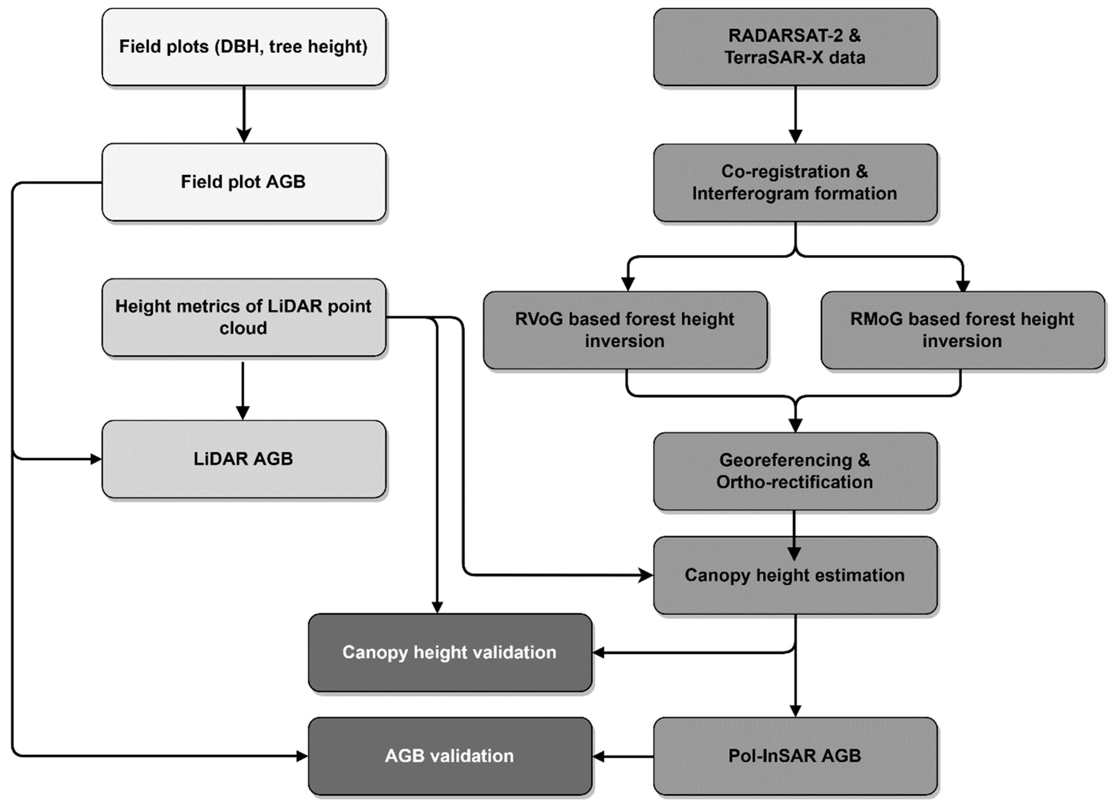
An overview of this study’s workflow is displayed in Figure 2. The applied steps are described in the following section in detail.

3.1. Extrapolated Reference Data

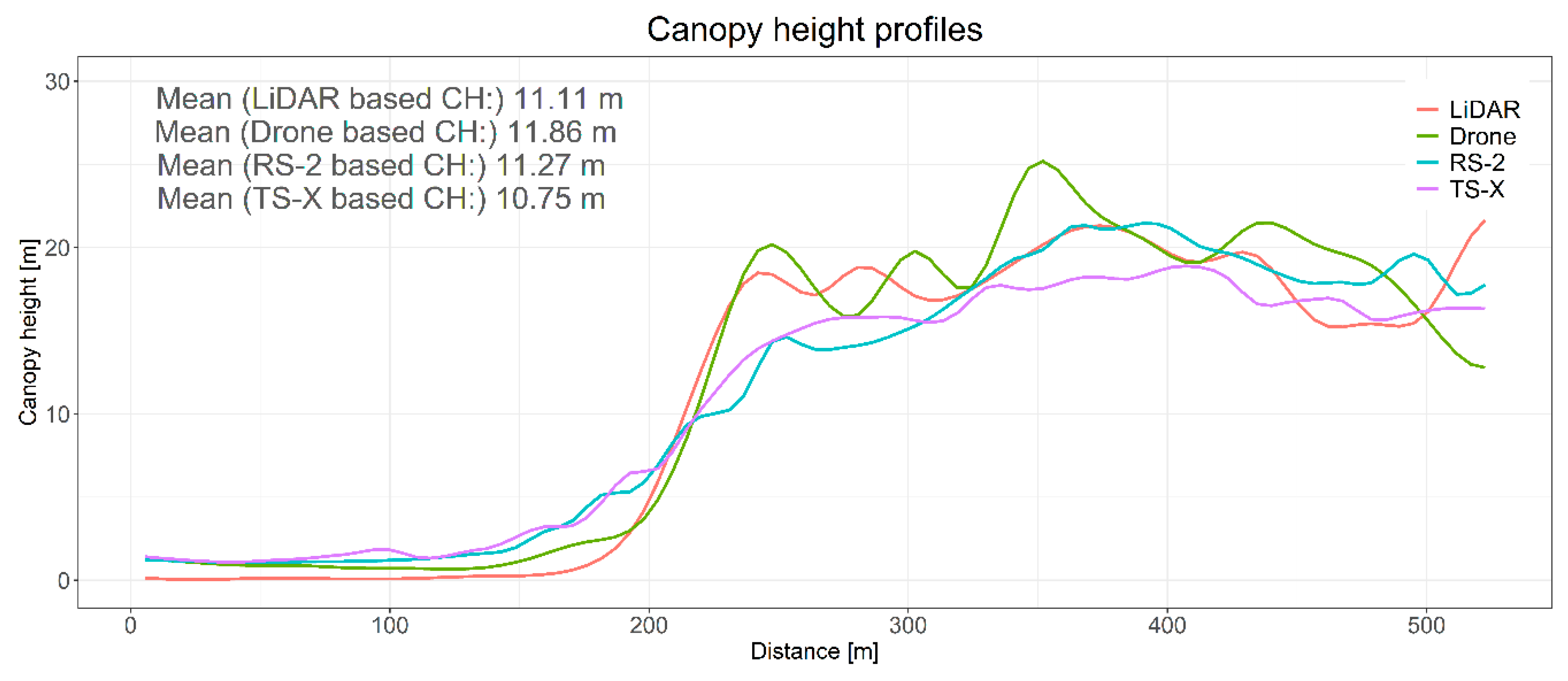
Canopy height from LiDAR data and AGB based on field inventory and LiDAR height metrics are used as reference data, representing the highest possible accuracy, for model calibration and validation. In a first step, a Digital Surface Model (DSM) was estimated from the hierarchical filtered highest points of the LiDAR point cloud. Besides, the DTM (Digital Terrain Model) with a resolution of 1 m was calculated from the filtered ground points of the 3D LiDAR point cloud [23,40]. By subtracting the DTM from the LiDAR DSM, a very accurate determination of the canopy height became possible. The final Canopy Height Model (CHM) based on LiDAR data has a spatial resolution of 1 m and is resampled to the respective Pol-InSAR data.

The field inventory data enabled the estimation of AGB in t ha⁻¹ by using the tree height, DBH, and wood specific density of each tree as the input for a combination of different allometric models. We applied allometric models according to [41] for saplings (DBH < 5 cm and height ≤ 1.3 m) and small trees (DBH < 5 cm and height > 1.3 m) and based on [42] for moist tropical forest stands (DBH ≥ 5 cm and height > 1.3 m). The applied models are described in detail in [24]. In a next step this ground-based AGB in t ha⁻¹ was related to the LiDAR transects in order to estimate AGB reference data based on centroid height derived from LiDAR using previously established regression models [23,24]. For each AGB grid cell, we computed the LiDAR height histograms by normalizing all points within a grid of 20 m (the same radius as the field plots) using the DTMs as ground reference as in [23,24]. The regression models are based on a combination of a power function in the lower biomass range and a linear function in the higher biomass range using the centroid height to calculate a certain threshold [24]. The centroid height is an appropriate height parameter of the LiDAR point cloud. The threshold of the centroid height was determined by increasing the value in steps of 0.001 m by identifying the lowest RMSE. The resolution of the final AGB map is 5 m and is resampled to the respective Pol-InSAR data. This extrapolating from field inventory data to LiDAR transects allows the creation of numerous biomass reference data for the calibration of SAR images.

In addition, inventory plots and surrounding areas were covered during a drone mission, approximately 270 ha. With the use of a Semi-Global Matching (SGM), a dense stereo-matching procedure, a 3D point cloud was created from the captured aerial photos. Similar to the LiDAR point cloud, a DSM was derived from this point cloud, which allowed a very precise determination of the canopy height minus the existing LiDAR DTM. We compared the unmanned aerial vehicle (UAV) derived canopy height to the LiDAR derived canopy height resulting in a correlation of 0.89.

3.2. SAR Processing

We applied a speckle reduction using the Refined Lee filter. Besides filtering, the co-registration of repeat pass SAR data is fundamental for generating an interferogram, as it ensures that a target on the ground corresponds to the same pixel in the master as in the slave image. This step compensates for different sensor attitudes, orbit crossings, along- and across track shifting and different sampling rates. After co-registrating the image pairs, we computed an interferogram, also called the phase difference, for each pixel. The interferogram of two registered complex images was calculated by the multiplication of one image with the conjugate of the second image [43].

In a next step, we smoothed the interferogram by using an adaptive filter based on the local fringe spectrum. The goal of the adaptive filter was to reduce phase noise, thereby reducing the number of residues. It read the complex valued interferogram, computed the interferogram power spectrum, designed a filter based on the power spectrum, filtered the interferogram, estimated the phase noise coherence value for the filtered interferogram and finally wrote the filtered interferogram.

3.3. Canopy Height Estimation

We tried two inversion models in order to estimate canopy height, the RVoG and the RMoG model. The RVoG model is a simple two-layer model, in which one layer represents the forest canopy and the other a reflective ground layer below the vegetation layer. It simulates vegetation as a homogeneous layer of thickness (h_v) containing volume scatterers with randomly oriented particles over a ground scatterer positioned at z. The model ignores the even-bounce scattering mechanism as well as higher order interactions. Pol-InSAR data is commonly used as input because it provides a number of independent parameters for modelling [26].

The RVoG presents the interferometric coherence $\tilde{\gamma }$ as

$$\tilde{\gamma }=exp\left(i{\mathsf{\phi }}_0\right)\frac{\widetilde{{\gamma }_v}+m}{1+m}$$

(1)

where φ₀ is the phase and refers to the topography of the ground, m is the effective ground-to-volume amplitude ratio. The complex coherence $\widetilde{{\gamma }_v}$ for the volume is given as [44,45,46]

$$\widetilde{{\gamma }_{\mathrm{v}}}=\frac{\mathrm{I}}{{\mathrm{I}}_0}\{\begin{array}{c}\mathrm{I}=\underset{0}{\overset{{\mathrm{h}}_{\mathrm{v}}}{{\displaystyle \int }}}\exp \left(\frac{2{\mathsf{\sigma }\mathrm{z}}^{\prime }}{{\cos \mathsf{\theta }}_0}\right)\exp \left({\mathrm{ik}}_{\mathrm{z}}\mathrm{z}\prime \right)\mathrm{d}\mathrm{z}\prime \\ {\mathrm{I}}_0=\underset{0}{\overset{\mathrm{hv}}{{\displaystyle \int }}}\exp \left(\frac{2{\mathsf{\sigma }\mathrm{z}}^{\prime }}{{\cos \mathsf{\theta }}_0}\right)\mathrm{d}\mathrm{z}\prime \end{array}$$

(2)

with ϴ₀ as the mean incidence angle, the assumption of an exponential distribution of all scatterers is a widely used approach, especially at higher frequencies such as X- and C-band [33]. $\widetilde{{\gamma }_v}$ depends on the extinction coefficient for the random volume σ and its thickness (h_v). The variable dz is defined as an independent distributed random variable that represent the physical displacement of scatterers along z. The effective vertical interferometric wavenumber k_z depends on the wavelength λ and the imaging geometry as the difference of the incidence angle Δϴ [44]

$$k_z=\frac{k\mathsf{\Delta }\theta }{sin{\theta }_0}\mathrm{with}k=\frac{4\pi }{\lambda }$$

(3)

The RMoG links the RVoG coherence model with the temporal coherence model and volumetric decorrelation to overcome those limitations [47]. The RMoG model separates temporal and volumetric decorrelations into four structural parameters and two dynamic parameters. The structural parameters are the tree height, wave extinction, ground topography and ground-to-volume ratio. The dynamic parameters are known as ground and canopy motion standard deviations induced by the temporal baseline [47].

The complex coherence ${\gamma }_M$ in the RMoG model is defined as

$${\gamma }_M=\frac{{{\displaystyle \int }}_0^{h_v}p\left(z\right)\exp \left(j{k}_{z}z\right)\left(-\frac{1}{2}{\left(\frac{4\pi }{\lambda }\right)}^2\right){\sigma }_r^2\left(z\right)dz}{{{\displaystyle \int }}_0^{h_v}p\left(z\right)dz}$$

(4)

where the scatterer motion function ${\sigma }_r^2$(z) is obtained from

$${\sigma }_r^2\left(\mathrm{z}\right)={\sigma }_g^2+\left({\sigma }_v^2-{\sigma }_g^2\right)\frac{z-z_g}{h_r},$$

(5)

with h_r as reference height, which is a constant, λ is the wavelength of the SAR system, and σ_g and σ_v are the ground and vegetation layer motion standard deviation. The term p(z) is the structure function defining the vertical structure of the vegetation layer [47,48]. The structure of trees is assumed as a Gaussian function.

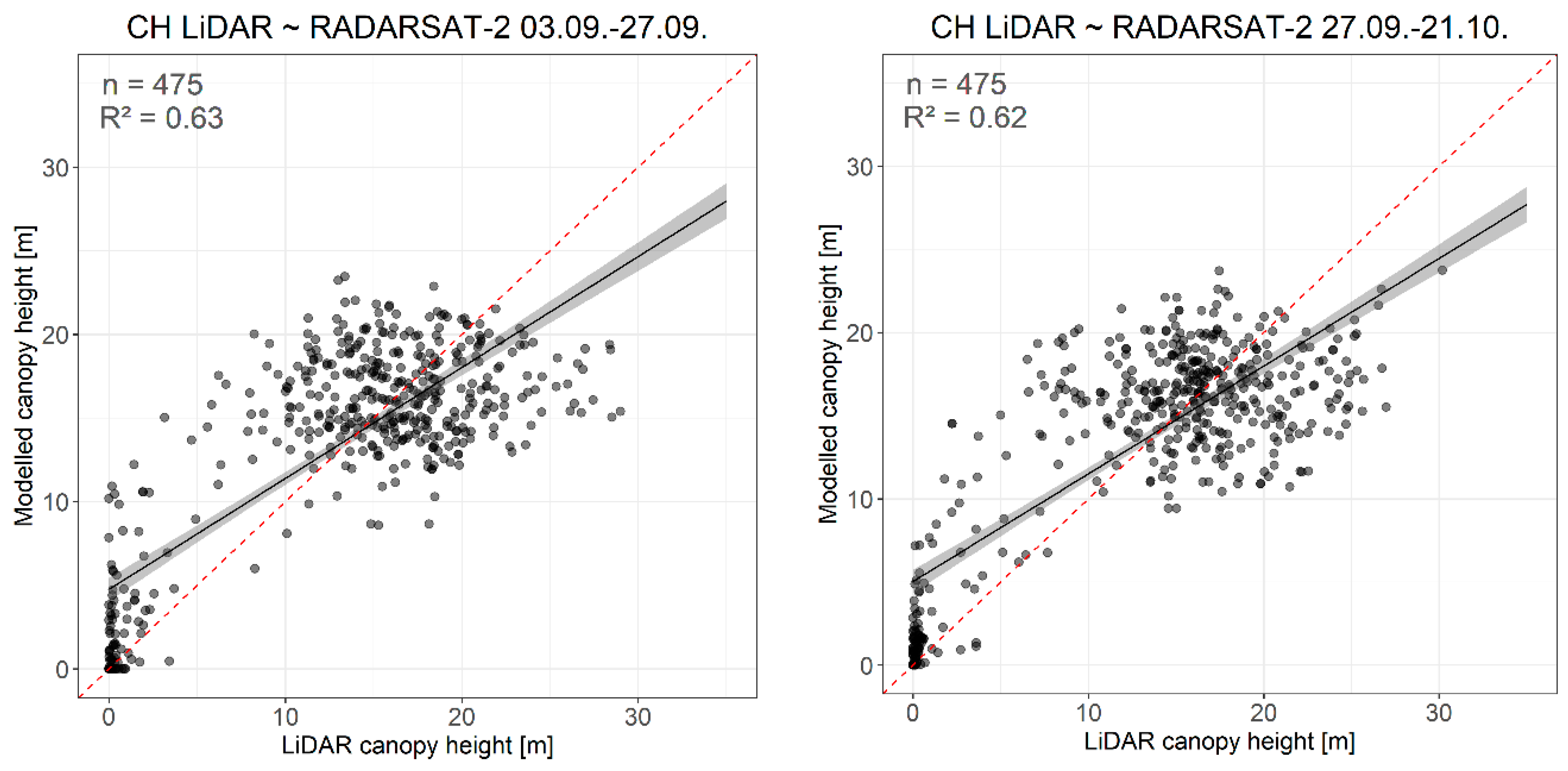
To compare the estimation results with each other as well as with the ground truth, we applied geo-referencing and ortho-rectifications. As a result, each pixel was mapped to a geographical location (longitude and latitude). After modelling the canopy height, an overestimation of the model was identified in the RS-2 results. For minimizing this overestimation, a linear correction factor of −1.4 m was applied on the final canopy height results of the RS-2 datasets.

3.4. SAR Based AGB Modelling

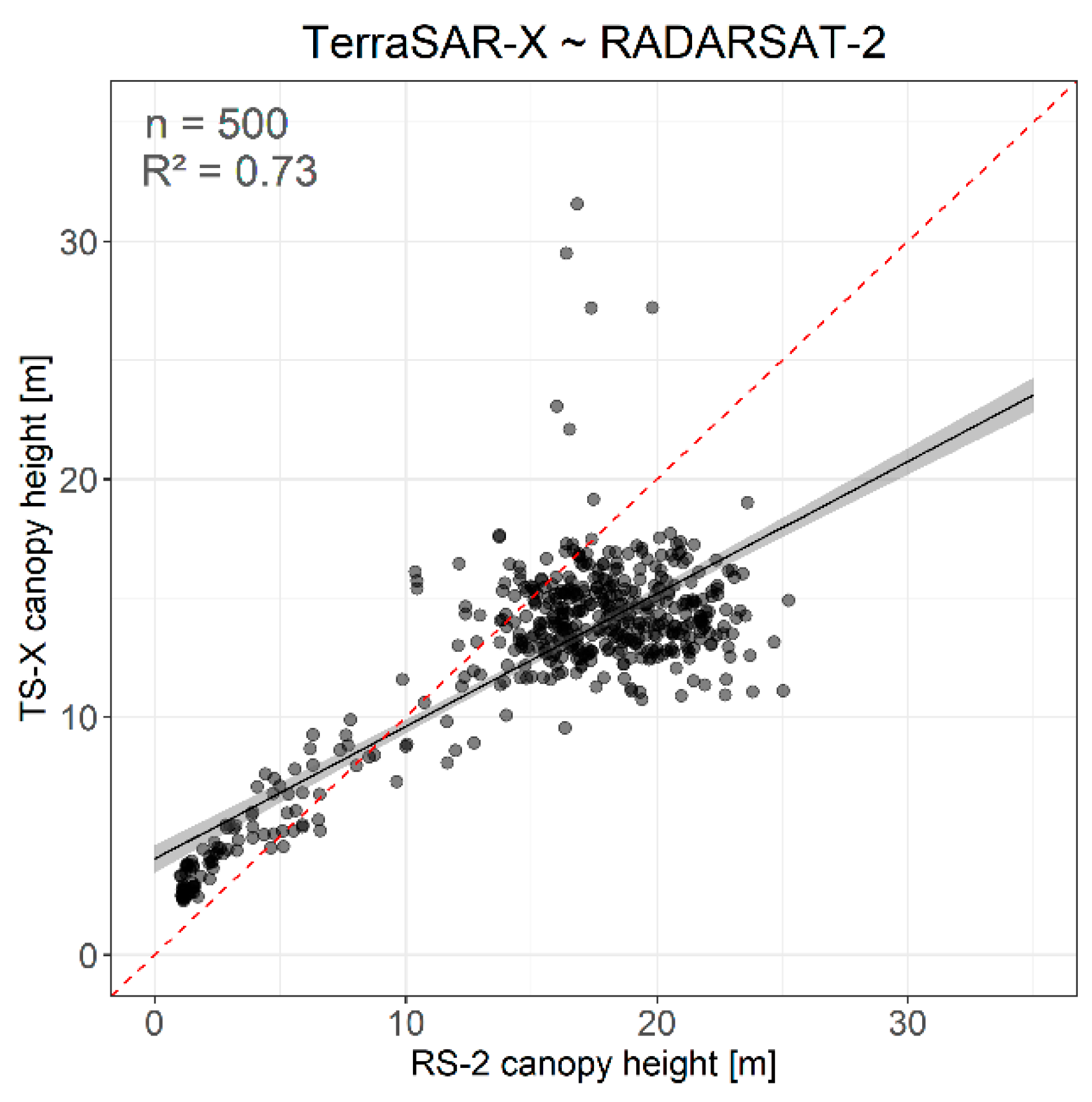
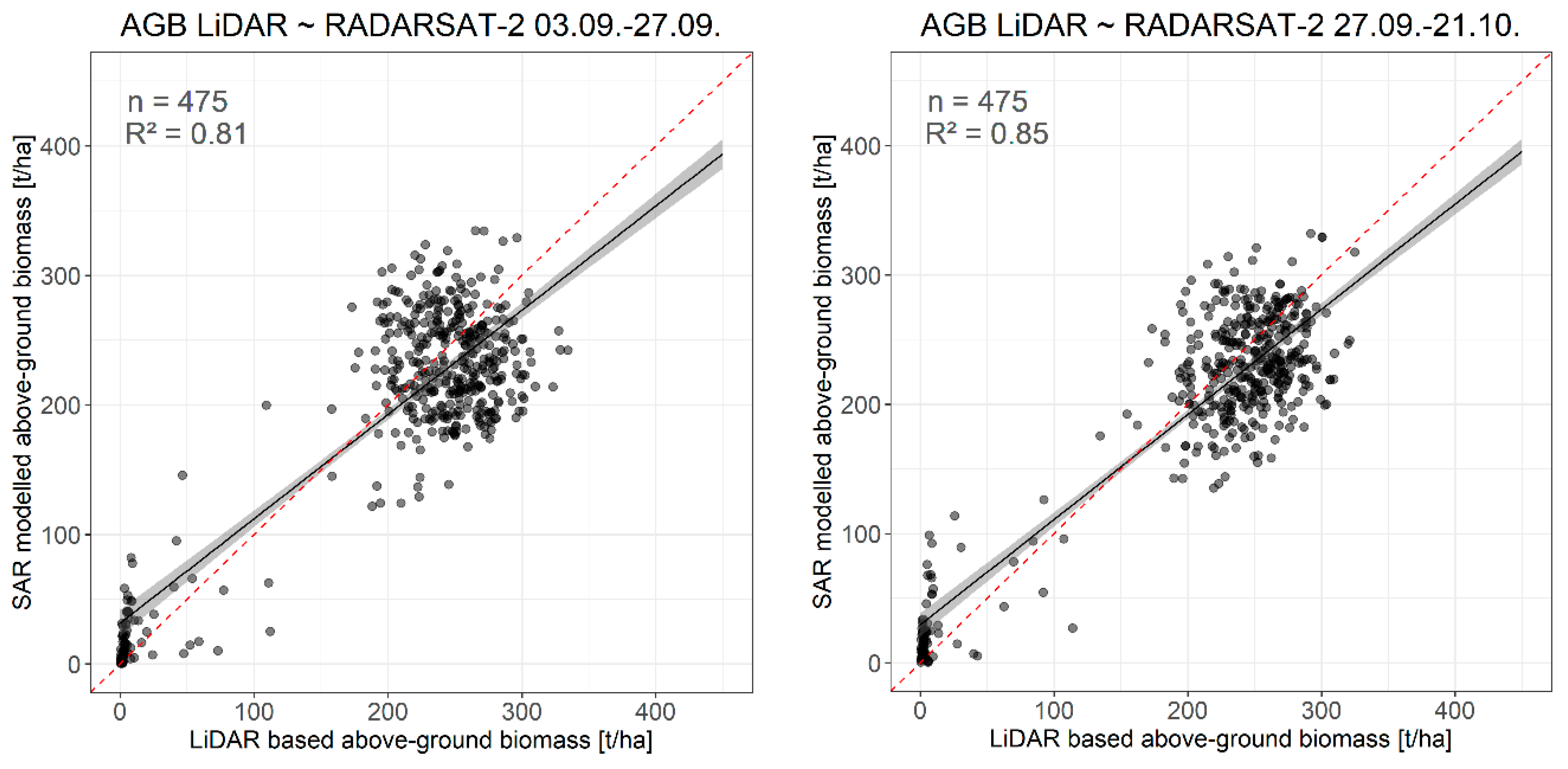
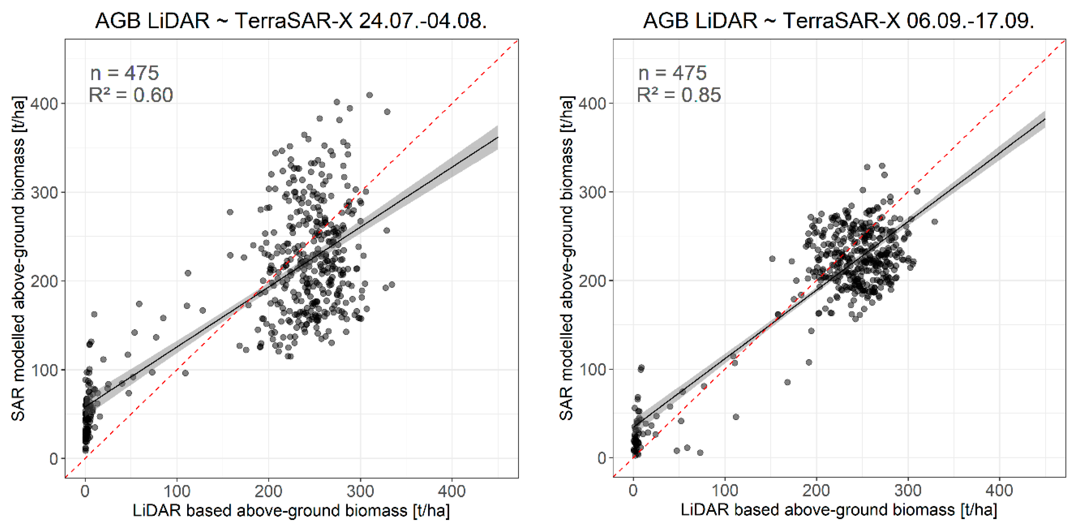
In a next step, we used Pol-InSAR based canopy height and LiDAR AGB as reference to set up a linear regression model for each scene based on 500 randomly selected pixels in the overlapping area. AGB was modelled for each scene based on the respective linear regression equation. Using the Cook’s distance (Cook’s D), influential outliers were removed from the set of predictor variables [49]. The Cook’s D identifies points with large residuals based on the observation’s leverage and the residual values, and thus influential outliers. Following this approach points over 4/n, where n is the number of observations, are removed from the modelling process [49]. The final resolution of the Pol-InSAR AGB maps is 3 and 12 m depending on the used sensor.

3.5. Validation

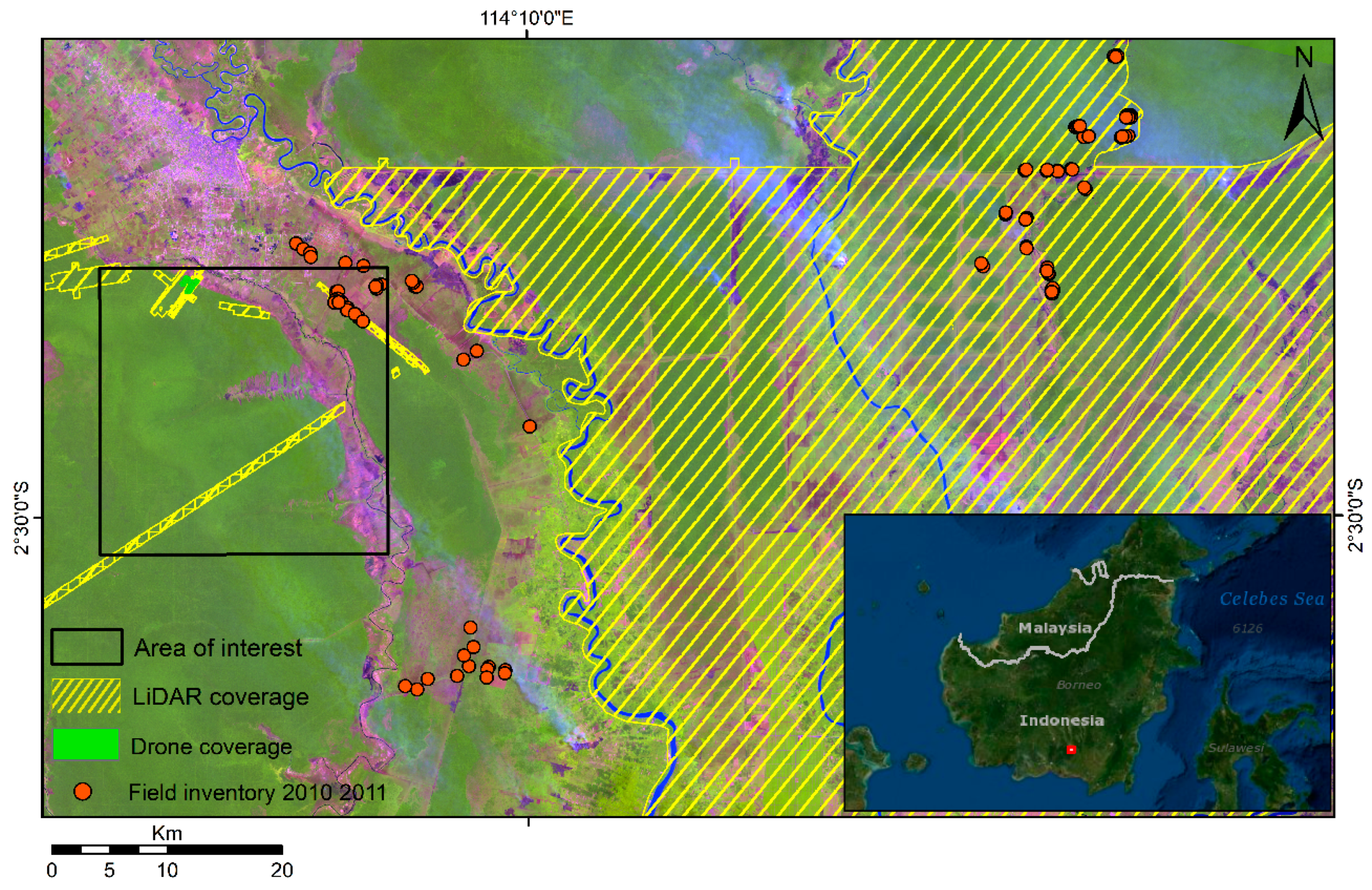
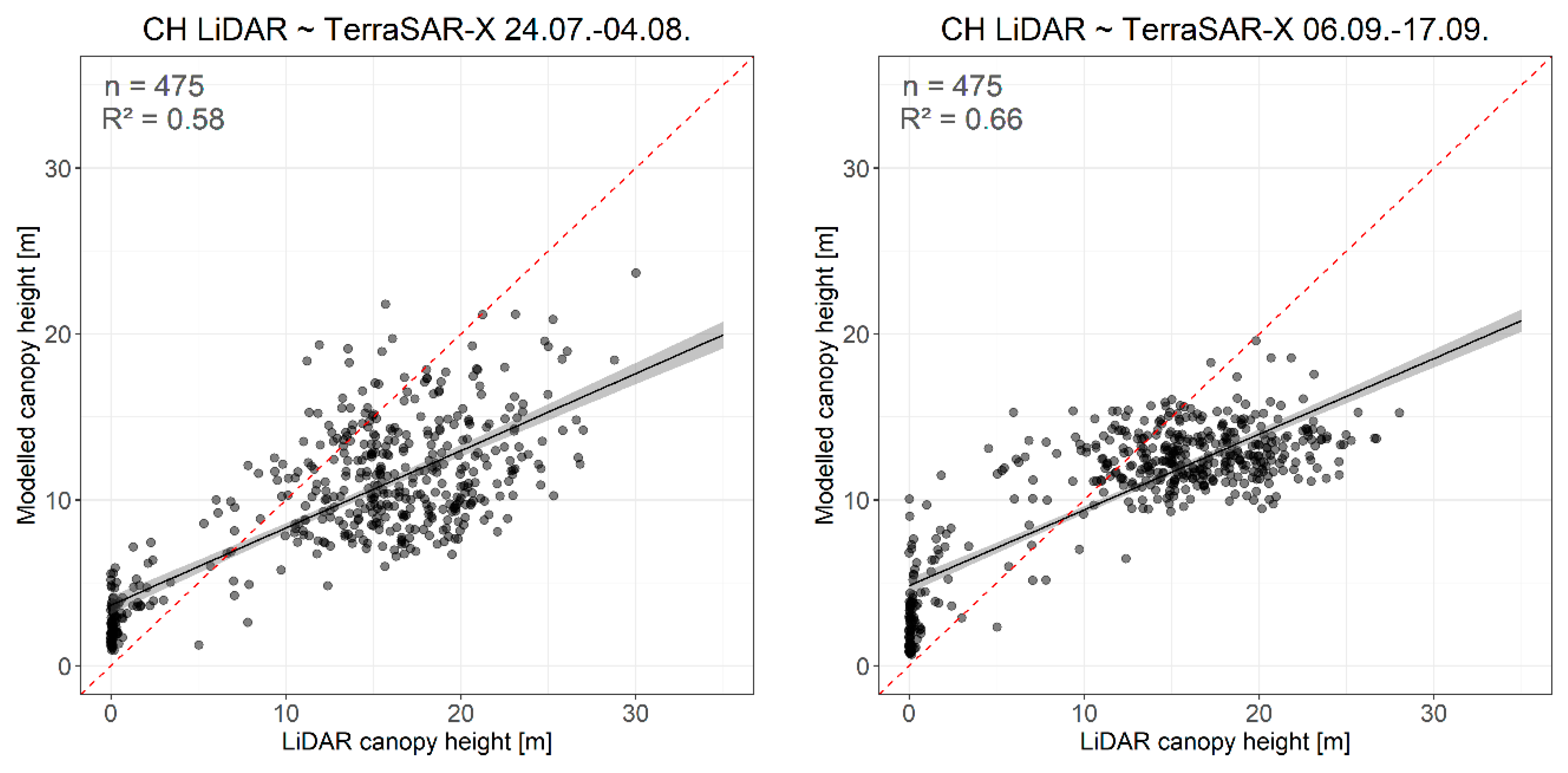
The validation of the estimated canopy height and modelled AGB is achieved using the reference data of the canopy height estimated from the drone DSM in combination with LiDAR DTM. A random sampling strategy was applied in ArcGIS (ESRI) to collect 475 randomly selected pixel within an overlapping area of the drone, as well as the LiDAR reference data and the modelled canopy height. Our drone data was acquired one year after the SAR data, and the LiDAR data was acquired four years before the SAR data. Nevertheless, the coverage of the drone data with the Pol-InSAR data is just about 270 ha. The LiDAR data on the other hand covers, depending on image, more than 4000 ha of the Pol-InSAR scenes. To overcome the limitations of the small coverage of the UAV data, the validation for canopy height is achieved based on both reference datasets within the respective overlapping areas. Since drone data is only available for canopy height, AGB is validated entirely with LiDAR modelled AGB. The resolution of the AGB validation datasets is resampled to the resolution of the respective SAR based canopy height and AGB map (3–12 m).

4. Results

4.1. RVoG vs. RMoG

For testing RVoG model-based inversion, we used six sets of RS-2 pairs from different beam-modes FQ3W (10.08. and 03.09., 27.09. and 21.10.), FQ7W (18.09. and 25.08., 18.09. and 12.10.) and FQ14W (11.09. and 18.08, 11.09. and 05.10.) as inputs for the RVoG and RMoG algorithms.

The RVoG model shows a strong overestimation in canopy height modelling in comparison to the LiDAR data in all tested datasets. An example for the modelling results using both inversion models is shown in Figure 3. The scatterplots show a strong overestimation of modelled canopy height using the RVoG model. The RMoG model demonstrates its superiority over the RVoG resulting in a more significant p-value and a higher R². As a result, we decided to use the better suitable RMoG model for estimating canopy height based on Pol-InSAR data in the following.

4.2. Canopy Height Estimation

In Figure 4, the canopy height of LiDAR, drone and two examples of RS-2 and TS-X based canopy height are displayed for a transect of approximately 500 m. The general pattern of the canopy height shows an appropriate overlap, but not all peaks match the reference height. The increase of the canopy height at a distance of 175 m results from a transition zone from non-forested area to forested area. The RS-2 based mean canopy height leads to an average overestimation of approximately 0.6 m compared to LiDAR reference and an underestimation of 0.16 m compared to the reference canopy height of the UAV. Mean tree height modelled from TS-X data is underestimated by 1.1 m compared to drone data and underestimated by 0.36 m in comparison to LiDAR canopy height. Both Pol-InSAR datasets tend to overestimate the canopy height in lower heights and underestimate in forested areas.

Figure 5 gives an overview of the correlation of the modelled canopy height based on Pol-InSAR data and the reference data based on LiDAR. The coefficient of determination (R²) for modelled canopy height from RS-2 varies between 0.62–0.63. The canopy height based on Pol-InSAR is overestimating heights ranging from 0–15 m and underestimates trees with heights taller than 15 m.

In Figure 6, the correlation of the reference and modelled canopy height based on TS-X is pointed out. The coefficient of determination varies from 0.58–0.66. Canopy heights modelled based on TS-X data result in an underestimation, whereby the image pair from July/August shows a stronger underestimation and a higher Root Mean Square Error (RMSE) than the interferogram estimated from two September images. A saturation effect can be identified at trees taller than 15 m.

In Figure 7, the differences between the modelling results of TS-X and RS-2 become clear. The correlation of the two sensors is strong until a canopy height of 10 m is reached. With increasing height, a stronger underestimation of TS-X in comparison to RS-2 is visible. At a height of approximately 15 m, a saturation effect in the TS-X data is monitored. For RS-2 the saturation effect can be identified at about 20 m.

In

Table 3. Validation statistics of canopy heights per interferogram based on LiDAR data. ($\overline{CH}$Ref = mean of the reference canopy height, $\overline{CH}$Est = mean of the estimated canopy height, SD = standard deviation, RMSE = root mean square error).

Sensor	Image Pair	${\overline{\mathit{C}\mathit{H}}}_{\mathbf{Ref}}\left[\mathbf{m}\right]$	${\overline{\mathit{C}\mathit{H}}}_{\mathbf{Est}}\left[\mathbf{m}\right]$	SDRef [m]	SDEst [m]	Bias [m]	R2	RMSE [m]
RS-2	10.08.–03.09.	14.04	15.86	7.09	5.49	1.8	0.54	5.12
	18.08.–11.09.	13.66	17.51	7.66	5.96	3.85	0.48	6.74
	25.08.–18.09.	13.51	16.73	7.59	6.68	3.22	0.57	5.99
	03.09.–27.09.*	13.08	13.43	7.61	6.36	0.35	0.63	4.65
	11.09.–05.10.	13.45	15.58	7.75	6.93	2.13	0.59	5.43
	18.09.–12.10.	13.43	13.62	7.69	6.31	0.18	0.60	4.88
	27.09 –21.10.*	13.36	13.68	7.43	6.13	0.32	0.62	4.62
	05.10.–29.10.	13.36	14.98	7.80	5.88	1.62	0.41	6.22
TS–X	13.07.–24.07.	Coherence too low for modelling
	24.07.–04.08.*	13.38	9.88	7.53	4.59	−3.5	0.58	6.10
	04.08.–15.08.	Coherence too low for modelling
	15.08.–26.08.	12.96	6.89	7.45	3.84	−6.07	0.39	8.44
	06.09.–17.09.*	13.06	10.79	7.43	4.16	−2.27	0.66	5.21

*datasets used for AGB modelling.

and

Table 4. Validation statistics of canopy heights per interferogram based on drone data. ($\overline{CH}$Ref = mean of the reference canopy height, $\overline{CH}$Est = mean of the estimated canopy height, SD = standard deviation, RMSE = root mean square error).

Sensor	Image Pair	${\overline{\mathit{C}\mathit{H}}}_{\mathbf{Ref}}\left[\mathbf{m}\right]$	${\overline{\mathit{C}\mathit{H}}}_{\mathbf{est}}\left[\mathbf{m}\right]$	SDRef [m]	SDEst [m]	Bias [m]	R2	RMSE [m]
RS-2	03.09.–27.09.	13.95	15.21	7.36	6.40	1.25	0.69	4.27
	27.09.–21.10.	13.91	15.03	7.34	6.08	1.12	0.65	4.47
TS-X	24.07.–04.08.	13.13	11.81	7.05	4.49	−1.31	0.55	4.95
	06.09.–17.09.	13.50	12.38	7.06	4.17	−1.12	0.68	4.43

, the validation statistics of the modelled canopy height are listed for both LiDAR and drone data. Each result was validated against the LiDAR and UAV canopy height using 475 collected random points, respectively. The LiDAR bias shows a slight overestimation of approximately 0.30–3.85 m for the modelled canopy height based on RS-2 and an underestimation (−3.5–−6.07 m) for the TS-X data (Table 3). The coefficient of determination varies in a range from 0.39–0.66 for the different results, showing the highest correlation for the TS-X interferogram in the date span of 06.09.–17.09. The standard deviation (SD) shows a higher value for the reference data than for the modelled data, meaning that the model does not adequately capture the canopy height range. The RMSE is about 4.65–6.74 m for RS-2 based canopy height and 5.2–8.44 m for TS-X based canopy height. Two TS-X datasets could not be modelled since the coherence was too low. The four results with the highest coefficient of determination were used to model AGB and to compare with the UAV data from 2016 (Table 4). The drone data has a smaller time lag towards the SAR data than the LiDAR data. Nevertheless, the area covered by drone data is very small. The results are comparable to the LiDAR data, the RMSE is slightly lower, varying from 4.27–4.95. The bias is smaller than for LiDAR data, especially for TS-X. Nevertheless, TS-X still shows an underestimation, while RS-2 is overestimating canopy height in average.

4.3. AGB Estimation

For AGB modelling, the datasets with the highest accuracy for the canopy height were used. The statistics of the linear regression models for modelling AGB in t ha⁻¹ based on the canopy height are summarized in

Table 5. Overview of the model statistics, adjusted R² and Residual Standard Error (RSE) for the linear regression AGB model based on canopy height.

Sensor	Image Pair	B	Std. Error	Beta	P Value	R2	RSE [t ha−1 ]
RS-2	03.09.–27.09.	14.3462	0.4306	33.31	<2e-16 ***	0.74	60.68
	27.09.–21.10.	14.516	0.469	30.952	<2e-16 ***	0.71	58.3
TS-X	24.07.–04.08.	21.2768	0.7791	27.309	< 2e-16 ***	0.66	63.67
	06.09.–17.09.	22.6038	0.6227	36.30	< 2e-16 ***	0.77	52.16

Signif. codes: 0 ‘***’ 0.001 ‘**’ 0.01 ‘*’ 0.05 ‘.’ 0.1 ‘ ’ 1.

. In addition, coefficient of determination and the residual standard error (RSE) are displayed for the different models. The R² varies between 0.66–0.77 and points out the ability of the model to predict AGB based on canopy height. In Figure 8 and Figure 9, the correlation of the reference and modelled AGB based on RS-2 and TS-X are pointed out. The coefficient of determination varies from 0.81–0.85 for RS-2 and from 0.60–0.85 for TS-X. RS-2 shows in general a better fit compared to the 1:1 line than the TS-X datasets. Both sensors tend to overestimate the AGB in lower biomass ranges and underestimate in higher biomass ranges. Estimated AGB from TS-X based on the datasets from 24.07.–04.08 depict a stronger scattering than the other datasets in the higher AGB range.

The validation of the modelled AGB using 475 random points resulted in the statistics summarized in

Table 6. Validation statistics of AGB per image pair.

Sensor	Image Pair	${\overline{\mathit{A}\mathit{G}\mathit{B}}}_{\mathbf{Ref}}\left[\mathbf{t}{\mathbf{ha}}^{-1}\right]$	${\overline{\mathit{A}\mathit{G}\mathit{B}}}_{\mathbf{est}}\left[\mathbf{t}{\mathbf{ha}}^{-1}\right]$	SDRef [t ha−1]	SDEst [t ha−1]	Bias [t ha−1]	R2	RMSE [t ha−1]
RS-2	03.09.–27.09.	197.30	188.05	100.64	95.83	−9.25	0.81	46.34
	27.09.–21.10.	198.14	188.02	100.10	93.68	−10.12	0.83	40.19
TS-X	24.07.–04.08.	196.94	191.08	100.49	87.82	−5.85	0.60	64.89
	06.09.–17.09.	196.44	181.48	99.19	93.44	−14.96	0.85	41.11

. R² varies from 0.66 to 0.84 showing a good agreement between the modelled AGB based on canopy height and the reference data. Nevertheless, the average AGB estimates are consistently lower than the reference biomass. The bias shows an underestimation of all four datasets and varies between 1.7% and 8.6%. Overall, the RMSE and coefficient of determination are similar in all datasets except for the TS-X data from July/August. This dataset shows higher deviations from the reference AGB than the other images. The relative RMSE varies from 20.2% to 23.3% for RS-2 datasets and from 20.9% to 32.9% for TS-X.

The comparison of different AGB maps shows the advantage of high-resolution images (Figure 10). The displayed wetland in the Sebangau National Park consists of a pattern of linearly vegetated and non-vegetated areas. TS-X with a resolution of 3 m is able to capture the pattern of the vegetation and its AGB better than existing maps. Even small-scaled variabilities and heterogeneities can be detected.

5. Discussion

5.1. Comparison of the RVoG and RMoG Models

The choice of different models has an effect on the resulting estimation result since the models differ in the in the number of input variables. The number of observables limits the complexity of the model meaning that the inversion process can be deterministic. However, a certain number of parameters is needed to deliver a good simulation of the scattering process. The RVoG model does not take the temporal baseline resulting from repeat-pass Pol-InSAR into consideration. However, the dynamic changes caused by wind, precipitations, seasonal variations and anthropogenic activities also lead to further decorrelation, altering the magnitude and phase of the observed coherence by an amount comparable to volumetric decorrelation.

Comparing the results of the two inversion models, the superiority of the RMoG model was pointed out. This is expected since the RVoG model does not take temporal decorrelation, introduced by the time gaps between acquisition dates, into consideration [47,48]. Especially the motion of scatterers, like wind motion of trees, results in lower coherences and inaccuracies in the canopy height estimation [52]. In addition, during this time period results of the inversion approach are not only affected by the motion of canopies but also by changes of dielectric properties [53]. Since all datasets of this study are multi-pass interferometric, temporal decorrelation is always present. The temporal baseline is about eleven days for TS-X and even 24 days for RS-2. As expected, the RMoG model demonstrates its capability to compensate parts of the temporal decorrelation.

5.2. Canopy Height Estimation

The results of the study indicate a suitability of Pol-InSAR C- and X-band data for canopy height modelling. The results of the different tested Pol-InSAR images against LiDAR and drone data varied since the acquisition parameters and the weather conditions changed during acquisitions. It can be concluded, that not all RS-2 and TS-X data is suitable for modelling canopy height from coherence. The parameters that most affect the canopy height model were identified as the baselines (temporal and perpendicular), the HoA, the incident angle and moist weather conditions, as well as the wavelength. Ascending and descending flight direction was not showing an influence. Nevertheless, our modelling results are comparable with several studies using InSAR and Pol-InSAR data for canopy height and AGB estimation. InSAR images at C-band were used by [54] to estimate stem volume and attained a RMSE value of 27%. Schlund et al. [55] modelled canopy height in boreal and temperate forests based on single-polarized TandDEM-X data. The authors used the RVoG model to estimate tree heights and validated their results with LiDAR data. The R² lied between 0.08–0.64 and the RMSE varied from 4.8 to 13.5 m [55]. Khati et al. [53] analyzed Indian tropical canopy heights based on TS-X/TanDEM-X data and attained RMSEs from 2.71–3.17 m for different seasons using the RVoG inversion approach. Other studies in tropical forests showed an average error between 3–5 m in estimating tree heights using Pol-InSAR likewise [56]. Kugler et al. [33] found an underestimation for tall forest stands and an overestimation for low canopy heights using dual-pol TanDEM-X data in Central Kalimantan, similar to our outcomes. Depending on rainy or dry season, their correlations (R²) varied between 0.55 and 0.69 for modelled canopy height based on the RVoG model [33]. Ghasemi et al. [48] modelled canopy height using P-band Pol-InSAR data and reached correlations of 0.43–0.48.

5.3. Possible Sources of Error

5.3.1. Acquisition Parameters

The quality of the interferogram is a useful parameter for determining the accuracy of the registration procedure. SAR data pairs may not be registered properly, if the resulting interferogram shows very little fringes and many decorrelated areas. However, co-registration of forested areas plays a crucial role within interferogram formation and leads to a low coherence. This low coherence in forests results from temporal decorrelation caused by wind effects in tree crowns. In the case of zero ground contribution, coherence becomes independent of polarization [44]. To overcome this limitation, a coherence optimization algorithm that accomplishes a pure signal-to-noise optimization is applied [57]. The coherence optimization allows selecting ground that gives the highest coherence under a random vegetation layer by maximizing the ground and minimizing the volume return [58].

Apart from the temporal baseline, the critical perpendicular baseline can cause decorrelation within an interferogram. The critical baseline is defined as the perpendicular baseline at which the interferometric correlation becomes zero and thus is completely decorrelated [53]. Longer wavelengths are less sensitive to decorrelation due to the perpendicular baseline as found in the comparison between X-and C-band. In general, the perpendicular baseline is inversely proportional to the HoA. A decreasing perpendicular baseline means an increasing HoA and results in a decreasing height sensitivity as shown in [59]. Nevertheless, for two TS-X datasets, the canopy height could not be estimated since the perpendicular baseline was too long and thus the HoA to low. The inversion process requires a HoA not smaller than the highest measured plot canopy height [53]. Since the HoA of two datasets was approximately 30 m and the tallest trees in the LiDAR reference data are about 35 m, an adequate inversion model performance was not possible.

The general underestimation of TS-X data results from the weak penetration depth, limited by the short wavelength of X-band [60]. Without this penetration capability, it is not possible to capture the canopy volume in the interferogram and the canopy estimation is restricted [33]. This means, the taller and denser the trees, the more saturated the canopy height estimation. The forests in Central Kalimantan are very dense and reach a height of up to 30 m, which limits the canopy height estimation. Alongside the density and height of the forest, the dielectric properties of the canopy also influence the penetration depth. The dataset of July/August were influenced by precipitation, consequently changing the dielectric properties of the forest.

Other studies found that the incidence angle also influences the canopy height inversion since the vertical wavenumber is estimated based on the incidence angle [61,62]. A smaller angle causes a larger vertical wavenumber relative to the effective baseline [61]. Using X-band and C-band with a weak penetration depth, a larger vertical wavelength can be sensitive to canopy height inversion. Additionally, very flat angles can cause radar shadows and introduce noise to the data [62].

With its longer wavelength the RS-2 data is able to penetrate the canopy layer more profoundly to capture the canopy volume in a more accurate way than TS-X. Nevertheless, TS-X has a better spatial resolution than RS-2 data, which enables the identification of small-scaled differences in the forest as e.g., because of logging. The fusion of RS-2 and TS-X was carried out to combine the complementary information of the two sensors in order to achieve better performance. However, due to difficulties in co-registering the two datasets originating from different sensors, and the general underestimation of TS-X X-band data, fusion did not result in enhanced performance.

5.3.2. Validation Datasets

The modelled canopy height was validated using UAV and LiDAR canopy height. Differences between LiDAR and drone data cannot only occur because of a temporal shift between the datasets, but also since estimations of canopy height vary between the different datasets. The performance of the photogrammetric products by drone can be influenced by structural complexity of a forest [63]. Nevertheless, UAV show good potential and derive similar results compared to LiDAR based canopy height R² = 0.89 which is consistent with results from [63].

Besides differences in acquisition parameters and weather conditions, another possible source of error is the four-year time shift between the LiDAR reference (2011) and the Pol-InSAR data (2015). Due to the offset of four years, differences resulting from deforestation and growing cannot be ruled out and are probable. Nevertheless, major changes during the four years can be excluded since the data was checked for fires and deforestation. Validating the modelled canopy height with drone data (2016) with a time shift of only one year resulted in higher correlations and lower biases and RMSEs for each dataset. However, area covered by the UAV data is very small, leading to the decision to include the LiDAR data for validation purposes to cover the whole range from low to high canopy height. Furthermore, no AGB data is available modelled from drone data, which is why the calibration and validation of AGB is based on LiDAR data.

Field and LiDAR data used as reference AGB also introduces errors, since spatial variability cannot be fully covered. The precision and accuracy of AGB extrapolated from field plot data are affected by the size and shape of the plots [64]. Most of the used field plots in the present study exceed an area of 1000 m², a size large enough to be more robust against boundary effects and less sensitive to individual trees [65,66,67]. Aside from the size, the shape affects the results of extrapolated AGB. Rectangular plots are more sensitive to the circumference to area ratio than circular plots [68]. As the count of rectangular plots is limited and only within single regrowing forest areas, their influence is marginal in the context of AGB estimation. In addition to the plot shape and size, the applied allometric model for moist tropical forests can introduce inaccuracies since it does not differentiate between different tree species [69]. We expect uncertainties using allometric equations varying from ±5 – ± 25% as shown in other studies [42,70]. The use of species-specific regression models is not realizable since tropical forests consist of hundreds of tree species. Nevertheless, the used information about wood specific densities and tree species from field plot data helps to overcome those limitations. By using the extrapolating approach from field plot to LiDAR AGB estimation for reference AGB estimation, the advantage is the enormous amount of data, covering all ranges of AGB. Furthermore, the data is representing the spatial variability in a more accurate way [17]. Even after the separation of the data into calibration and validation samples, the use of a large number of samples is guaranteed. The results of the validation are thus more accurate than in studies with a more limited amount of in-situ data.

5.4. AGB Estimation

AGB can be estimated based on the canopy height [48,71,72]. Extrapolating from field inventory data to LiDAR transects allows creating numerous biomass reference data for the calibration of SAR images. Furthermore, it allows estimating AGB across large areas and different ecosystems taking in account the advantage of mapping the spatial variability of AGB. The estimated AGB from Pol-InSAR derived canopy height showed good correlations compared to reference canopy height. For AGB modelling based on canopy height, most studies use a power function regression. The use of linear regression in this context has been confirmed in few studies [73,74]. Nevertheless, testing both regression models with our data resulted in significant p-values for both regressions but higher R² and lower RMSE using a linear regression.

To overcome the inaccuracies introduced by the time gap between the LiDAR and the Pol-InSAR data, the Cook’s D was applied. This standard measure of influence allows to remove influential outlier identified by a combination of observation leverages and residual values [75]. Using the Cook’s D, we analyzed each dataset of 500 variables regarding outliers that can influence the linear regression AGB model. Per dataset 1–2% of the variables were identified as influential outliers and removed from the linear regression modelling. In most cases, the identified variables were pixel, where forest was degraded within the time gap of four years.

The comparison with pan-tropical biomass maps as seen in [36,50,51,76] with a resolution of 100 m–1 km in general showed a good consistency of the AGB estimates. Baccini et al. [51], using field data from 2007–2008 and LiDAR waveform measurements from NASA’s ICESat, showed an overestimation in lower biomass ranges. The map is not able identifying heterogeneity in tropical forests in detail because of its coarse resolution of 500 m. The map of Saatchi et al. [76] also tends to underestimate high biomass values but represents disturbances better due to its spatial resolution of 250 m. Avitabile et al. [36] used the maps of [76] and [51] with additional data to create an improved biomass map in the pan-tropical region. This final map shows lower RMSE and bias than the previous studies. Nevertheless, the map with its spatial resolution of 1 km does not capture small heterogeneities and disturbances. Berninger et al. [50] produced AGB maps of Kalimantan with a spatial resolution of 100 m, preserving small scale disturbances and regrowing effects for different years. The RMSE varies between 53–57 t ha⁻¹ and relative RMSE from 31–8%. Other studies using L- and P-band, estimated AGB with RMSE values between 30–40% for L-band and between 20–30% for P-band for boreal forests [77,78]. We obtained a relative RMSE for biomass between 20–30% using X- and C-band but with a much finer resolution of 3–12 m. Similar to the results of the present study, all of the pan-tropical and Indonesian maps underestimate higher AGB ranges and overestimate lower AGB values [36].

6. Conclusions

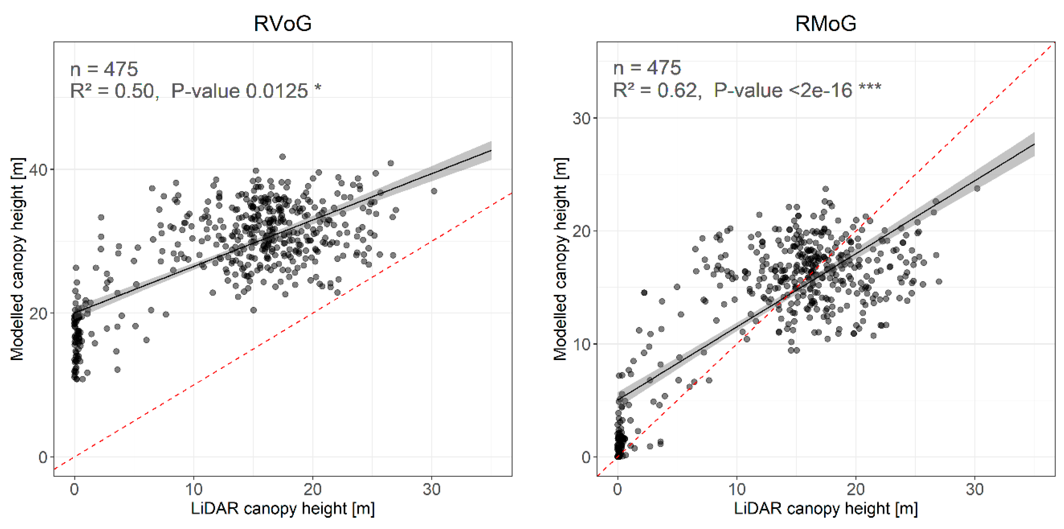
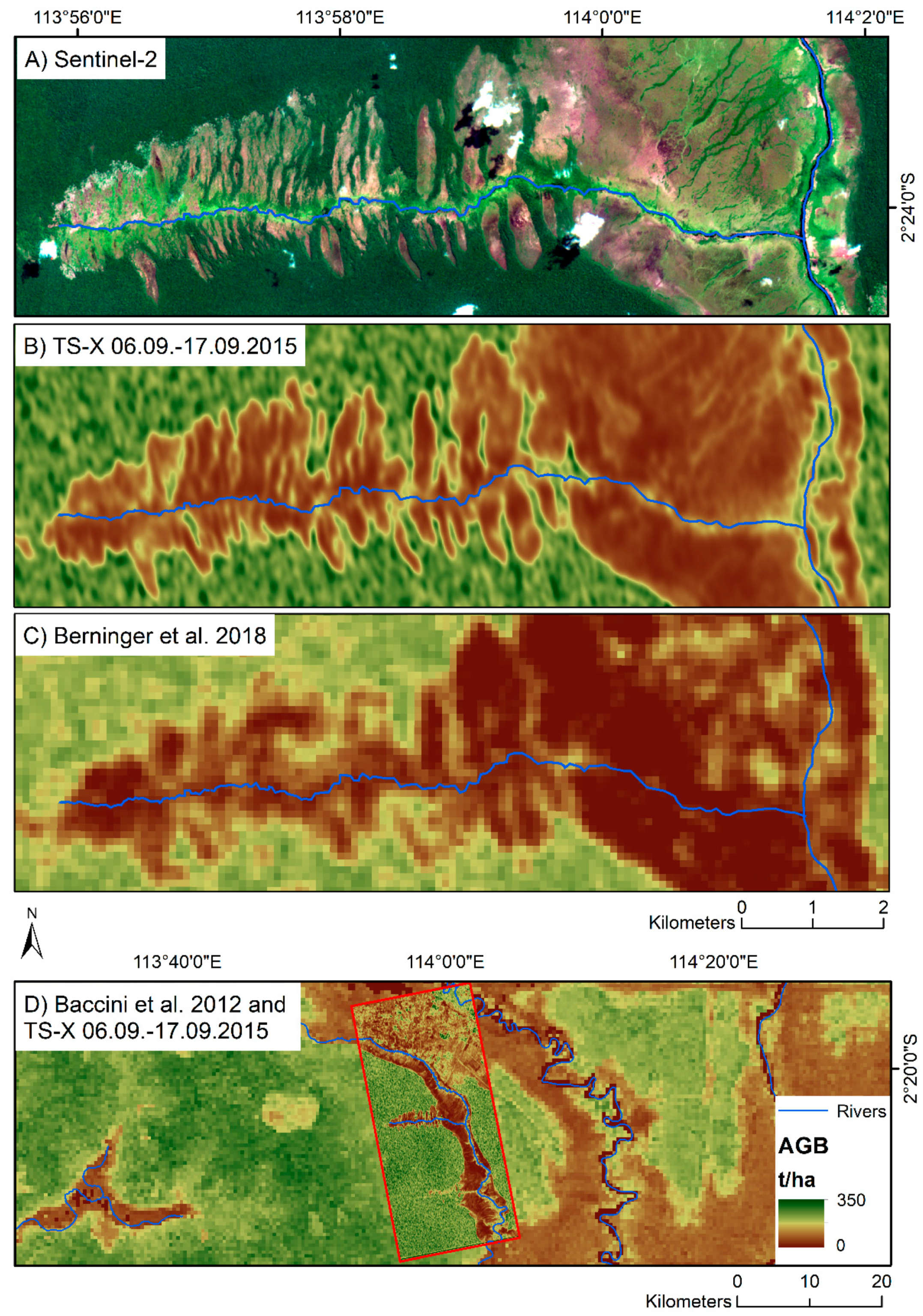
The results of the study show the suitability of Pol-InSAR RS-2 and TS-X data for canopy height estimation in tropical forests of Indonesia using the RMoG model (i). Since all data utilized are multi-pass interferometric data, temporal decorrelation is always present. While the RMoG model demonstrated good potential for compensating temporal decorrelation, this was not addressed in the RVoG model. Regression models were successfully applied for modelling large-scale AGB based on Pol-InSAR canopy height (ii). The validation of all modelled canopy heights and AGB values using the RMoG model was achieved using extensive LiDAR and drone reference data. The results of the different tested images varied since the acquisition parameters and the weather conditions changed during acquisitions. It was shown that canopy height is slightly underestimated by TS-X, whereas RS-2 overestimates the canopy height. Both sensors underestimate AGB, which can be explained with the saturation effect of SAR data regarding biomass. However, a combined canopy height estimation did not provide enhanced performance.

High-resolution information about canopy height and biomass is important for carbon accounting. Since the collection of field data is time-consuming and not practicable in all areas of the world, the use of LiDAR, drone and satellite data are helpful alternatives. Nevertheless, LiDAR and drone data acquisitions are very cost-intensive. The use of earth observation approaches enables a cost-effective way to cover large areas. Moreover, the high data availability and the combination of different sensors enables the reduction of uncertainties in indirect measurement approaches such as canopy height and biomass modelling from SAR data. We showed that the RMoG can help to estimate high-resolution canopy height data and AGB from different sensors and thus allows a support to monitoring and risk managing systems for spacious areas. The resulting outcomes contribute to REDD+ and other carbon related projects. Future missions such as Tandem-L (DLR) and the Earth Explorer Biomass (ESA) help to further improve data availability for biomass estimation.

References

1. World Bank Group. Forest Area (% of Land Area): Indonesia. Available online: https://data.worldbank.org/indicator/AG.LND.FRST.ZS?end=2015&locations=IDtart=2015&type=shaded&view=map&year=2010 (accessed on 14 February 2019).
2. Pachauri, R.K.; Meyer, L.A. IPCC 2014. Climate change 2014. Synthesis report. Contribution of Working Groups I, II and III to the Fifth Assessment Report of the Intergovernmental Panel on Climate Change; Core Writing Team, Pachauri, R.K., Meyer, L.A., Eds.; Intergovernmental Panel on Climate Change: Geneva, Switzerland, 2015; ISBN 9291691437. [Google Scholar]
3. Page, S.E.; Rieley, J.O.; Banks, C.J. Global and regional importance of the tropical peatland carbon pool. Glob. Chang. Biol. 2011, 17, 798–818. [Google Scholar] [CrossRef] [Green Version]
4. Jaenicke, J.; Rieley, J.O.; Mott, C.; Kimman, P.; Siegert, F. Determination of the amount of carbon stored in Indonesian peatlands. Geoderma 2008, 147, 151–158. [Google Scholar] [CrossRef]
5. Edwards, D.P.; Koh, L.P.; Laurance, W.F. Indonesia’s REDD+ pact: Saving imperilled forests or business as usual? Biol. Conserv. 2012, 151, 41–44. [Google Scholar] [CrossRef]
6. Olivier, J.G.J.; Janssens-Maenhout, G.; Muntean, M.; Peters, J.A.H.W. Trends in Global CO2 Emissions: 2015 Report. 2015. Available online: https://edgar.jrc.ec.europa.eu/news_docs/jrc-2015-trends-in-global-co2-emissions-2015-report-98184.pdf (accessed on 26 February 2019).
7. Global Canopy Foundation. The REDD Desk. Available online: https://theredddesk.org/countries/search-countries-database?f%5B0%5D=type%3Aactivity&f%5B1%5D=field_project%3A1 (accessed on 7 February 2018).
8. Goetz, S.; Dubayah, R. Advances in remote sensing technology and implications for measuring and monitoring forest carbon stocks and change. Carbon Manag. 2011, 2, 231–244. [Google Scholar] [CrossRef]
9. FAO. Assessment of the Status of the Development of the Standards for the Terrestrial Essential Climate Variables. 2009. Available online: http://www.fao.org/3/i1238e/i1238e00.pdf (accessed on 6 February 2019).
10. Bojinski, S.; Verstraete, M.; Peterson, T.C.; Richter, C.; Simmons, A.; Zemp, M. The Concept of Essential Climate Variables in Support of Climate Research, Applications, and Policy. Bull. Am. Meteorol. Soc. 2014, 95, 1431–1443. [Google Scholar] [CrossRef]
11. Koch, B. Status and future of laser scanning, synthetic aperture radar and hyperspectral remote sensing data for forest biomass assessment. ISPRS J. Photogramm. Remote Sens. 2010, 65, 581–590. [Google Scholar] [CrossRef]
12. Joshi, N.; Mitchard, E.T.A.; Schumacher, J.; Johannsen, V.K.; Saatchi, S.; Fensholt, R. L-Band SAR Backscatter Related to Forest Cover, Height and Aboveground Biomass at Multiple Spatial Scales across Denmark. Remote Sens. 2015, 7, 4442–4472. [Google Scholar] [CrossRef] [Green Version]
13. Schlund, M.; Poncet, F.; Kuntz, S.; Schmullius, C.; Hoekman, D.H. TanDEM-X data for aboveground biomass retrieval in a tropical peat swamp forest. Remote Sens. Environ. 2014, 158, 255–266. [Google Scholar] [CrossRef]
14. Asner, G.P.; Clark, J.K.; Mascaro, J.; Galindo García, G.A.; Chadwick, K.D.; Navarrete Encinales, D.A.; Paez-Acosta, G.; Cabrera Montenegro, E.; Kennedy-Bowdoin, T.; Duque, Á.; et al. High-resolution mapping of forest carbon stocks in the Colombian Amazon. Biogeosciences 2012, 9, 2683–2696. [Google Scholar] [CrossRef] [Green Version]
15. Asner, G.P.; Flint Hughes, R.; Varga, T.A.; Knapp, D.E.; Kennedy-Bowdoin, T. Environmental and Biotic Controls over Aboveground Biomass Throughout a Tropical Rain Forest. Ecosystems 2009, 12, 261–278. [Google Scholar] [CrossRef]
16. Solberg, S.; Astrup, R.; Gobakken, T.; Næsset, E.; Weydahl, D.J. Estimating spruce and pine biomass with interferometric X-band SAR. Remote Sens. Environ. 2010, 114, 2353–2360. [Google Scholar] [CrossRef]
17. Englhart, S.; Keuck, V.; Siegert, F. Aboveground biomass retrieval in tropical forests—The potential of combined X- and L-band SAR data use. Remote Sens. Environ. 2011, 115, 1260–1271. [Google Scholar] [CrossRef]
18. Duncanson, L.I.; Niemann, K.O.; Wulder, M.A. Estimating forest canopy height and terrain relief from GLAS waveform metrics. Remote Sens. Environ. 2010, 114, 138–154. [Google Scholar] [CrossRef]
19. Zhao, K.; Popescu, S.; Nelson, R. Lidar remote sensing of forest biomass: A scale-invariant estimation approach using airborne lasers. Remote Sens. Environ. 2009, 113, 182–196. [Google Scholar] [CrossRef]
20. Kronseder, K.; Ballhorn, U.; Böhm, V.; Siegert, F. Above ground biomass estimation across forest types at different degradation levels in Central Kalimantan using LiDAR data. Int. J. Appl. Earth Obs. Geoinf. 2012, 18, 37–48. [Google Scholar] [CrossRef]
21. Asner, G.P.; Powell, G.V.N.; Mascaro, J.; Knapp, D.E.; Clark, J.K.; Jacobson, J.; Kennedy-Bowdoin, T.; Balaji, A.; Paez-Acosta, G.; Victoria, E.; et al. High-resolution forest carbon stocks and emissions in the Amazon. Proc. Natl. Acad. Sci. USA 2010, 107, 16738–16742. [Google Scholar] [CrossRef] [Green Version]
22. Ballhorn, U.; Jubanski, J.; Siegert, F. ICESat/GLAS Data as a Measurement Tool for Peatland Topography and Peat Swamp Forest Biomass in Kalimantan, Indonesia. Remote Sens. 2011, 3, 1957–1982. [Google Scholar] [CrossRef] [Green Version]
23. Jubanski, J.; Ballhorn, U.; Kronseder, K.; Franke, J.; Siegert, F. Detection of large above-ground biomass variability in lowland forest ecosystems by airborne LiDAR. Biogeosciences 2013, 10, 3917–3930. [Google Scholar] [CrossRef] [Green Version]
24. Englhart, S.; Jubanski, J.; Siegert, F. Quantifying Dynamics in Tropical Peat Swamp Forest Biomass with Multi-Temporal LiDAR Datasets. Remote Sens. 2013, 5, 2368–2388. [Google Scholar] [CrossRef] [Green Version]
25. Sun, X.; Song, H.J. A New Improved Algorithm Based on Three-Stage Inversion Procedure of Forest Height. In Proceedings of the 2015 14th International Symposium on Distributed Computing and Applications for Business Engineering and Science (DCABES), Guiyang, China, 18–24 August 2015; Available online: https://0-dl-acm-org.brum.beds.ac.uk/citation.cfm?id=2917944 (accessed on 26 February 2019).
26. Olesk, A.; Praks, J.; Antropov, O.; Zalite, K.; Arumäe, T.; Voormansik, K. Interferometric SAR Coherence Models for Characterization of Hemiboreal Forests Using TanDEM-X Data. Remote Sens. 2016, 8, 700. [Google Scholar] [CrossRef]
27. Lavalle, M.; Simard, M.; Hensley, S. A Temporal Decorrelation Model for Polarimetric Radar Interferometers. IEEE Trans. Geosci. Remote Sens. 2012, 50, 2880–2888. [Google Scholar] [CrossRef]
28. Garestier, F.; Dubois-Fernandez, P.C.; Papathanassiou, K.P. Pine Forest Height Inversion Using Single-Pass X-Band PolInSAR Data. IEEE Trans. Geosci. Remote Sens. 2008, 46, 59–68. [Google Scholar] [CrossRef]
29. Neumann, M.; Ferro-Famil, L.; Reigber, A. Multibaseline Polarimetric SAR Interferometry Coherence Optimization. IEEE Geosci. Remote Sens. Lett. 2008, 5, 93–97. [Google Scholar] [CrossRef]
30. Kugler, F. Pol-InSAR Forest Height estimation at different Frequencies: Oppertunities and Limitations. 2015. Available online: https://elib.dlr.de/102764/1/Dissertation-Florian-Kugler.pdf (accessed on 22 May 2019).
31. Hajnsek, I.; Hoekman, D.H. INDREX-II Indonesian Radar Experiment Campaign over Tropical Forest in L- and P-band. In Proceedings of the 2005 IEEE International Geoscience and Remote Sensing Symposium (IGARSS), Seoul, Korea, 29 July 2005; Volume 6, pp. 4335–4338. Available online: https://0-ieeexplore-ieee-org.brum.beds.ac.uk/document/1525878 (accessed on 30 April 2019).
32. Hajnsek, I.; Kugler, F.; Lee, S.K.; Papathanassiou, K.P. Tropical-Forest-Parameter Estimation by Means of Pol-InSAR: The INDREX-II Campaign. IEEE Trans. Geosci. Remote Sens. 2009, 47, 481–493. [Google Scholar] [CrossRef] [Green Version]
33. Kugler, F.; Schulze, D.; Hajnsek, I.; Pretzsch, H.; Papathanassiou, K.P. TanDEM-X Pol-InSAR Performancefor forest height estimation. IEEE Trans. Geosci. Remote Sens. 2014, 52, 6404–6422. [Google Scholar] [CrossRef]
34. Vyjayanthi, N.; Jha, C.S.; Murthy, M.S.R. Forest Biomass Estimation and Forest Structure Analysis from Multi-Frequency and Multi-Polarization SAR Data. RISAT-JEP. 2017. Available online: https://www.climatelinks.org/file/4121/download?token=WzORdftr (accessed on 22 April 2019).
35. Varekamp, C.; Hoekman, D.H. High-resolution InSAR image simulation for forest canopies. IEEE Trans. Geosci. Remote Sens. 2002, 40, 1648–1655. [Google Scholar] [CrossRef]
36. Avitabile, V.; Herold, M.; Heuvelink, G.B.M.; Lewis, S.L.; Phillips, O.L.; Asner, G.P.; Armston, J.; Ashton, P.S.; Banin, L.; Bayol, N.; et al. An integrated pan-tropical biomass map using multiple reference datasets. Glob. Chang. Biol. 2016, 22, 1406–1420. [Google Scholar] [CrossRef]
37. Page, S.E.; Rieley, J.O.; Wüst, R. Lowland tropical peatlands of Southeast Asia. Peatl. Evol. Rec. Environ. Clim. Chang. 2006, 9, 145–172. [Google Scholar] [CrossRef]
38. Raison, J.; Atkinson, P.; Chave, J.; Defries, R.; Joo, G.K.; Joosten, H.; Konecny, K.; Navratil, P.; Siegert, F. The High Carbon Stock Science Study - Independent Report from the Technical Committee: 2015. Available online: https://www.tfa2020.org/en/publication/high-carbon-stock-science-study/ (accessed on 23 May 2019).
39. Pearson, T.; Walker, S.; Brown, S. Sourcebook for Land Use, Land-Use Change and Forestry Projects. Available online: https://theredddesk.org/resources/sourcebook-land-use-land-use-change-and-frestry-projects (accessed on 1 December 2017).
40. Pfeifer, N.; Stadler, P.; Briese, C. Derivation of digital terrain models in SCOP++ environment. In Proceedings of the OEEPE Workshop on Airborne Laserscanning and Interferometric SAR for Digital Elevation Models, Stockholm, Sweden, 1–3 March 2001; pp. 1–13. Available online: http://citeseerx.ist.psu.edu/viewdoc/download?doi=10.1.1.589.8666&rep=rep1&type=pdf (accessed on 19 April 2019).
41. Hughes, R.F.; Kauffman, J.B.; Jaramillo, V.J. Biomass, Carbon, and Nutrient Dynamics of Secondary Forests in a Humid Tropical Region of Mexico. Ecology 1999, 80, 1892–1907. [Google Scholar] [CrossRef]
42. Chave, J.; Andalo, C.; Brown, S.; Cairns, M.A.; Chambers, J.Q.; Eamus, D.; Fölster, H.; Fromard, F.; Higuchi, N.; Kira, T.; et al. Tree allometry and improved estimation of carbon stocks and balance in tropical forests. Oecologia 2005, 145, 87–99. [Google Scholar] [CrossRef]
43. Moreira, A.; Prats-Iraola, P.; Younis, M.; Krieger, G.; Hajnsek, I.; Papathanassiou, K.P. A tutorial on synthetic aperture radar. IEEE Geosci. Remote Sens. Mag. 2013, 1, 6–43. [Google Scholar] [CrossRef] [Green Version]
44. Papathanassiou, K.P.; Cloude, S.R. Single-baseline polarimetric SAR interferometry—Geoscience and Remote Sensing, IEEE Transactions on. IEEE Trans. Geosci. Remote Sens. 2001, 39, 2352–2363. [Google Scholar] [CrossRef]
45. Treuhaft, R.N.; Madsen, S.N.; Moghaddam, M.; van Zyl, J.J. Vegetation characteristics and underlying topography from interferometric radar. Radio Sci. 1996, 31, 1449–1485. [Google Scholar] [CrossRef]
46. Treuhaft, R.N.; Siqueira, P.R. Vertical structure of vegetated land surfaces from interferometric and polarimetric radar. Radio Sci. 2000, 35, 141–177. [Google Scholar] [CrossRef] [Green Version]
47. Lavalle, M.; Hensley, S. Extraction of Structural and Dynamic Properties of Forests From Polarimetric-Interferometric SAR Data Affected by Temporal Decorrelation. IEEE Trans. Geosci. Remote Sens. 2015, 53, 4752–4767. [Google Scholar] [CrossRef]
48. Ghasemi, N.; Tolpekin, V.; Stein, A. Assessment of Forest Above-Ground Biomass Estimation from PolInSAR in the Presence of Temporal Decorrelation. Remote Sens. 2018, 10, 815. [Google Scholar] [CrossRef]
49. Cook, R.D. Detection of Influential Observation in Linear Regression. Technometrics 1977, 19, 15–18. [Google Scholar]
50. Berninger, A.; Lohberger, S.; Stängel, M.; Siegert, F. SAR-Based Estimation of Above-Ground Biomass and Its Changes in Tropical Forests of Kalimantan Using L- and C-Band. Remote Sens. 2018, 10, 831. [Google Scholar] [CrossRef]
51. Baccini, A.; Goetz, S.J.; Walker, W.S.; Laporte, N.T.; Sun, M.; Sulla-Menashe, D.; Hackler, J.; Beck, P.S.A.; Dubayah, R.; Friedl, M.A.; et al. Estimated carbon dioxide emissions from tropical deforestation improved by carbon-density maps. Nat. Clim. Chang. 2012, 2, 182–185. [Google Scholar] [CrossRef]
52. Lee, S.K.; Kugler, F.; Papathanassiou, K.P.; Moreira, A. Forest Height Estimation by Means of Pol-InSAR. Limitations Posed by Temporal Decorrelation. K&C Science Report—Phase 1. 2017. Available online: https://www.semanticscholar.org/paper/Forest-Height-Estimation-by-means-of-Pol-InSAR-by-Lee-Kugler/a7efde9c825e84e6cd927faab417425fccef9840 (accessed on 24 May 2017).
53. Khati, U.; Singh, G.; Ferro-Famil, L. Analysis of seasonal effects on forest parameter estimation of Indian deciduous forest using TerraSAR-X PolInSAR acquisitions. Remote Sens. Environ. 2017, 199, 265–276. [Google Scholar] [CrossRef]
54. Askne, J.; Santoro, M. Experiences in Boreal Forest Stem Volume Estimation from Multitemporal C-Band InSAR. Recent Interferometry Applications in Topography and Astronomy. Available online: https://pdfs.semanticscholar.org/2bc3/54b863ecf3a7b6cb6f250bf2a5c63bd8f051.pdf (accessed on 10 April 2019).
55. Schlund, M.; Magdon, P.; Eaton, B.; Aumann, C.; Erasmi, S. Canopy height estimation with TanDEM-X in temperate and boreal forests. Int. J. Appl. Earth Obs. Geoinf. 2019, 82, 101904. [Google Scholar] [CrossRef]
56. Arnaubec, A.; Dubois-Fernandez, P.C. Analysis of PolInSAR Precision for Forest and Ground Parameters Estimation in Tropical Context. In Proceedings of the 2012 IEEE International Geoscience and Remote Sensing Symposium (IGARSS), Munich, Germany, 22–27 July 2012; pp. 7585–7588. [Google Scholar]
57. Fomena, R.T.; Cloude, S.R. On The Role of Coherence Optimization in Polarimetric SAR Interferometry. CEOS 05 2005, 22, 9. [Google Scholar]
58. Tharaoui, S.; Ouarzeddine, M.; Souissi, B. Interferometric coherence optimization: A comparative Study. In Proceedings of the Eighth International Conference on Broadband and Wireless Computing, Communication and Applications (BWCCA), Compiègne, France, 28–30 October 2013; IEEE: Piscataway, NJ, USA, 2013. Available online: https://0-ieeexplore-ieee-org.brum.beds.ac.uk/xpl/conhome/6689793/proceeding (accessed on 15 April 2019).
59. Soja, M.; Ulander, L. Digital Canopy Model Estimation from TanDEM-X Interferometry using High-Resolution Lidar DEM, Melbourne, VIC, Australia, 21–26 July 2013. Available online: https://0-ieeexplore-ieee-org.brum.beds.ac.uk/document/6721117 (accessed on 11 April 2019).
60. Schlund, M.; Erasmi, S.; Scipal, K. Comparison of Aboveground Biomass Estimation From InSAR and LiDAR Canopy Height Models in Tropical Forests. IEEE Geosci. Remote Sens. Lett. 2019, 1–5. [Google Scholar] [CrossRef]
61. Sun, X.; Wang, B.; Xiang, M.; Jiang, S.; Fu, X. Forest Height Estimation Based on Constrained Gaussian Vertical Backscatter Model Using Multi-Baseline P-Band Pol-InSAR Data. Remote Sens. 2018, 11, 42. [Google Scholar] [CrossRef]
62. Hajnsek, I.; Scheiber, R.; Keller, M.; Horn, R.; Lee, S.; Ulander, L.; Gustavson, A.; Sandberg, G.; Le Toan, T.; Tebaldini, S.; et al. BIOSAR 2008 Technical Assistance for the Development of Airborne SAR and Geophysical Measurements during the BioSAR 2008 Experiment. Final Report. 2008. Available online: https://earth.esa.int/c/document_library/get_file?folderId=21020&name=DLFE-903.pdf (accessed on 21 June 2019).
63. Jayathunga, S.; Owari, T.; Tsuyuki, S. Evaluating the Performance of Photogrammetric Products Using Fixed-Wing UAV Imagery over a Mixed Conifer–Broadleaf Forest: Comparison with Airborne Laser Scanning. Remote Sens. 2018, 10, 187. [Google Scholar] [CrossRef]
64. Frazer, G.W.; Magnussen, S.; Wulder, M.A.; Niemann, K.O. Simulated impact of sample plot size and co-registration error on the accuracy and uncertainty of LiDAR-derived estimates of forest stand biomass. Remote Sens. Environ. 2011, 115, 636–649. [Google Scholar] [CrossRef]
65. Ruiz, L.; Hermosilla, T.; Mauro, F.; Godino, M. Analysis of the Influence of Plot Size and LiDAR Density on Forest Structure Attribute Estimates. Forests 2014, 5, 936–951. [Google Scholar] [CrossRef] [Green Version]
66. Rafael, M.N.C.; Eduardo, G.F.; Jorge, G.G.; Carlos, J.; Ceacero, R.; Rocío, H.C. Impact of plot size and model selection on forest biomass estimation using airborne LiDAR: A case study of pine plantations in southern Spain. J. For. Sci. 2017, 63, 88–97. [Google Scholar] [CrossRef]
67. Kachamba, D.; Ørka, H.; Næsset, E.; Eid, T.; Gobakken, T. Influence of Plot Size on Efficiency of Biomass Estimates in Inventories of Dry Tropical Forests Assisted by Photogrammetric Data from an Unmanned Aircraft System. Remote Sens. 2017, 9, 610. [Google Scholar] [CrossRef]
68. Mauya, E.W.; Hansen, E.H.; Gobakken, T.; Bollandsås, O.M.; Malimbwi, R.E.; Næsset, E. Effects of field plot size on prediction accuracy of aboveground biomass in airborne laser scanning-assisted inventories in tropical rain forests of Tanzania. Carbon Balanc. Manag. 2015, 10, 10. [Google Scholar] [CrossRef]
69. Urbazaev, M.; Thiel, C.; Cremer, F.; Dubayah, R.; Migliavacca, M.; Reichstein, M.; Schmullius, C. Estimation of forest aboveground biomass and uncertainties by integration of field measurements, airborne LiDAR, and SAR and optical satellite data in Mexico. Carbon Balanc. Manag. 2018, 13, 5. [Google Scholar] [CrossRef] [PubMed]
70. Saatchi, S.; Marlier, M.; Chazdon, R.L.; Clark, D.B.; Russell, A.E. Impact of spatial variability of tropical forest structure on radar estimation of aboveground biomass. Remote Sens. Environ. 2011, 115, 2836–2849. [Google Scholar] [CrossRef]
71. Lefsky, M.A.; Harding, D.J.; Keller, M.; Cohen, W.B.; Carabajal, C.C.; Del Bom Espirito-Santo, F.; Hunter, M.O.; de Oliveira, R. Estimates of forest canopy height and aboveground biomass using ICESat. Geophys. Res. Lett. 2005, 32. [Google Scholar] [CrossRef] [Green Version]
72. Feliciano, E.A.; Wdowinski, S.; Potts, M.D.; Lee, S.K.; Fatoyinbo, T.E. Estimating Mangrove Canopy Height and Above-Ground Biomass in the Everglades National Park with Airborne LiDAR and TanDEM-X Data. Remote Sens. 2017, 9, 702. [Google Scholar] [CrossRef]
73. Odipo, V.; Nickless, A.; Berger, C.; Baade, J.; Urbazaev, M.; Walther, C.; Schmullius, C. Assessment of Aboveground Woody Biomass Dynamics Using Terrestrial Laser Scanner and L-Band ALOS PALSAR Data in South African Savanna. Forests 2016, 7, 294. [Google Scholar] [CrossRef]
74. Köhler, P.; Huth, A. Towards ground-truthing of spaceborne estimates of above-ground life biomass and leaf area index in tropical rain forests. Biogeosciences 2010, 7, 2531–2543. [Google Scholar] [CrossRef] [Green Version]
75. Zakaria, A. On the Detection of Influential Outliers in Linear Regression Analysis. AJTAS 2014, 3, 100. [Google Scholar] [CrossRef]
76. Saatchi, S.S.; Harris, N.L.; Brown, S.; Lefsky, M.; Mitchard, E.T.A.; Salas, W.; Zutta, B.R.; Buermann, W.; Lewis, S.L.; Hagen, S.; et al. Benchmark map of forest carbon stocks in tropical regions across three continents. Proc. Natl. Acad. Sci. USA 2011, 108, 9899–9904. [Google Scholar] [CrossRef] [Green Version]
77. Soja, M.J.; Sandberg, G.; Ulander, L.M.H. Regression-Based Retrieval of Boreal Forest Biomass in Sloping Terrain Using P-Band SAR Backscatter Intensity Data. IEEE Trans. Geosci. Remote Sens. 2013, 51, 2646–2665. [Google Scholar] [CrossRef]
78. Sandberg, G.; Ulander, L.M.H.; Fransson, J.E.S.; Holmgren, J.; Le Toan, T. L- and P-band backscatter intensity for biomass retrieval in hemiboreal forest. Remote Sens. Environ. 2011, 115, 2874–2886. [Google Scholar] [CrossRef]
Figure 1. RGB composite of Landsat-8 (short-wave infrared, near-infrared, red) from 2015 showing the location of the area of interest including the field plots from 2010–2011 and the LiDAR (2011) and UAV (2016) coverage.
Remotesensing 11 02105 g001
Figure 2. Workflow of the methodology applied in this study (bright grey = field data, grey = LiDAR data, medium dark grey = SAR data, dark grey = validation).
Remotesensing 11 02105 g002
Figure 3. Correlation of reference LiDAR canopy height and modelled RS-2 canopy height for the RVoG (left) and RMoG (right) based on an interferogram from 27.09.-21.10. Dashed line = 1:1 line.
Remotesensing 11 02105 g003
Figure 4. Example height profile of reference LiDAR canopy height, drone canopy height, modelled RS-2 canopy height based on the interferogram from 03.09.-27.09 and modelled canopy height based on TS-X from 06.09.-17.09.
Remotesensing 11 02105 g004
Figure 5. Correlation of reference LiDAR canopy height and modelled RS-2 canopy height using RMoG model based on an interferogram from 03.09.–27.09. (left) and 27.09.–21.10. (right). Red dashed line = 1:1 line; black line = linear trend including confidence bounds.
Remotesensing 11 02105 g005
Figure 6. Correlation of reference LiDAR canopy height and modelled TS-X canopy height using RMoG model based on an interferogram from 24.07.–04.08. (left) and 06.09.–17.09. (right). Red dashed line = 1:1 line; black line = linear trend including confidence bounds.
Remotesensing 11 02105 g006
Figure 7. Correlation of modelled TS-X (06.09.–17.09.) canopy height and modelled RS-2 (03.09.–27.09.) canopy height based on the RMoG model. Red dashed line = 1:1 line; black line = linear trend including confidence bounds.
Remotesensing 11 02105 g007
Figure 8. Correlation of reference LiDAR AGB and modelled RS-2 AGB based on an interferogram from 03.09.–27.09. (left) and 27.09.–21.10. (right). Red dashed line = 1:1 line; black line = linear trend including confidence bounds, n = 475.
Remotesensing 11 02105 g008
Figure 9. Correlation of reference LiDAR AGB and modelled TS-X AGB based on an interferogram from 24.07.–04.08. (left) and 06.09.–17.09. (right). Red dashed line = 1:1 line; black line = linear trend including confidence bounds.
Remotesensing 11 02105 g009
Figure 10. Comparison between different biomass maps. (A) True-color image of Sentinel-2 showing a wetland in the Sebangau National Park, Central Kalimantan. (B) AGB with a resolution of 3 m modelled based on TerraSAR-X images from 06.09.-17.09.2015. (C) AGB with a resolution of 100 m, modelled by Berninger et al. [50] using ALOS PALSAR and Sentinel-1 from 2015. (D) AGB with a resolution of 500 m, modelled by Baccini et al. [51] based on ICE-Sat data from 2007 through 2008 and the TS-X based AGB results are from 06.09.–17.09.2015 (framed in red).
Remotesensing 11 02105 g010