Improved Estimates of Geocenter Variability from Time-Variable Gravity and Ocean Model Outputs


1
NASA Goddard Space Flight Center, Cryospheric Sciences Laboratory, Greenbelt, MD 20771, USA
2
Department of Earth System Science, University of California, Irvine, CA 92697, USA
3
Jet Propulsion Laboratory, California Institute of Technology, Pasadena, CA 91109, USA
*
Author to whom correspondence should be addressed.
†
Current address: Polar Science Center, Applied Physics Laboratory, University of Washington, Seattle, WA 98105, USA.
Remote Sens. 2019, 11(18), 2108; https://0-doi-org.brum.beds.ac.uk/10.3390/rs11182108
Submission received: 7 August 2019
/
Revised: 3 September 2019
/
Accepted: 4 September 2019
/
Published: 10 September 2019
(This article belongs to the Special Issue Remote Sensing by Satellite Gravimetry)
Abstract
:Geocenter variations relate the motion of the Earth’s center of mass with respect to its center of figure, and represent global-scale redistributions of the Earth’s mass. We investigate different techniques for estimating of geocenter motion from combinations of time-variable gravity measurements from the Gravity Recovery and Climate Experiment (GRACE) and GRACE Follow-On missions, and bottom pressure outputs from ocean models. Here, we provide self-consistent estimates of geocenter variability incorporating the effects of self-attraction and loading, and investigate the effect of uncertainties in atmospheric and oceanic variation. The effects of self-attraction and loading from changes in land water storage and ice mass change affect both the seasonality and long-term trend in geocenter position. Omitting the redistribution of sea level affects the average annual amplitudes of the x, y, and z components by 0.2, 0.1, and 0.3 mm, respectively, and affects geocenter trend estimates by 0.02, 0.04 and 0.05 mm/yr for the the x, y, and z components, respectively. Geocenter estimates from the GRACE Follow-On mission are consistent with estimates from the original GRACE mission.
1. Introduction
Variations in the Earth’s geocenter reflect the largest scale variability of mass within the Earth system, and are essential inclusions for the complete recovery of surface mass change from time-variable gravity [1,2]. The Earth’s geocenter is the difference between the Earth’s center of mass and center of figure, which is represented by the degree one spherical harmonic terms [3,4]. Estimates of geocenter position have important applications in the determination of terrestrial reference frame variations, satellite altimeter orbit fluctuations, and mass transport from time-variable gravity [1,5]. Geocenter positions are not stationary. Variations in geocenter have been attributed to changes in terrestrial water storage, glacier and ice sheet mass, atmospheric and oceanic circulation, geodynamic processes and other mass transport processes, Figure 1 [1,6,7,8].
Measurements of time-variable gravity from the Gravity Recovery and Climate Experiment (GRACE) and the GRACE Follow-On (GRACE-FO) missions are set in a center of mass (CM) reference frame, in which the total degree one variations are inherently zero [9,10,11]. However, the individual contributions to degree one variations in the CM reference frame, such as from oceanic processes or terrestrial water storage change, are not necessarily zero [4]. Applications set in a center of figure (CF) reference frame, such as the recovery of mass variations of the oceans, hydrosphere and cryosphere, also require the inclusion of degree one terms to be fully accurate [2,4]. The exclusion of degree one terms can have a significant impact on estimates of ocean mass [12], ice sheet mass change [13] and terrestrial hydrology [14] due to far-field signals leaking into each regional estimate.
There are presently two methods that regularly provide estimates of geocenter variability: (1) measurements from satellite laser ranging (SLR) [5,15] and (2) calculations from time-variable gravity and ocean model outputs [2,16]. Global inversions of GRACE data, GPS data, and modeled ocean bottom pressure can also provide long-term or detrended estimates of geocenter variability [17,18]. Trends in SLR-derived solutions can be contaminated by network effects, such as station drift [19,20]. They are not necessarily related to long-term changes in geocenter position. Geocenter estimates from inversions of time-variable gravity and ocean model outputs can provide trend estimates. However, they require information about the oceanic redistribution of mass from changes in terrestrial water storage and ice mass change [2]. Here, we improve geocenter estimates from time-variable gravity and ocean model output combinations by including the effects of self-attraction and loading. We test the overall sensitivity of the estimates to uncertainties in atmospheric pressure, ocean bottom pressure and glacial isostatic adjustment. In the following sections, we discuss (1) the data utilized for this research, (2) how we implement and test our method, (3) the results from our method and (4) the overall implications of the research.
2. Data
2.1. Time-Variable Gravity
We use monthly GRACE/GRACE-FO Release-6 (RL06) gravity solutions provided by the University of Texas Center for Space Research (UTCSR), the German Research Centre for Geosciences (GeoForschungsZentrum, GFZ) and the Jet Propulsion Laboratory (JPL) for the period April 2002–May 2019 [9,10,11,21]. Each Level-2 gravity field solution consists of fully-normalized spherical harmonic coefficients (, ) of degree, l, and order, m. We substitute the coefficients derived from GRACE/GRACE-FO data with estimates from satellite laser ranging (SLR) from NASA Goddard Space Flight Center due to anomalous variability in the GRACE-derived coefficients [22]. For periods when the satellite pairs had a single fully-operating accelerometer, we replace the coefficients derived from GRACE/GRACE-FO data with SLR-derived estimates [22]. The monthly GRACE/GRACE-FO RL06 products have non-tidal atmospheric mass variability removed using outputs from the European Centre for Medium-Range Weather Forecasts (ECMWF) and ERA-Interim [23]. Non-tidal oceanic mass variability is removed from the Release-6 GRACE/GRACE-FO data using outputs from the Max Planck Institute ocean model (MPIOM) [24]. We correct for the effects of Glacial Isostatic Adjustment (GIA), which is the viscoelastic response to changes in ice mass since the last glacial maximum, using outputs from the A et al. [25] compressible Earth model using ICE-6G ice history. The impact of different ice histories and mantle rheologies are tested using expected GIA rates from Caron et al. [26]. We account for the elastic deformation of the solid Earth induced by variations in surface mass loading using load Love numbers of gravitational potential, , calculated by Wahr et al. [27]. The degree one load Love number of gravitational potential, , is updated to reflect the use of a CF reference frame [28]. We smooth the GRACE/GRACE-FO coefficients using a 300 km radius Gaussian averaging function to reduce the impact of random spherical harmonic errors [4,29]. We filter the coefficients to reduce the impact of correlated north/south “striping” errors [30].
As an independent assessment of geocenter variability, we use monthly estimates derived from satellite laser ranging (SLR) [15]. The traditional SLR-derived geocenter solutions reflect the best fit to the center of the SLR network (CN) [31]. However, SLR-derived solutions can be affected by network-effects when individual stations drift relative to each other due to tectonics, surface loading or other processes [19]. Here, we use both the traditional CN-CM solutions [15] and the new UTCSR CF-CM solutions that try to account for these network-effect range biases [5]. We correct both sets of SLR solutions for the gravitational effects of non-tidal atmospheric and oceanic variability using the 6-h Release-6 de-aliasing product provided by GFZ [23].
2.2. Atmospheric Reanalyses and Ocean Models
We estimate the effect of uncertainty in atmospheric pressure by comparing the geocenter outputs from the GRACE/GRACE-FO atmospheric de-aliasing products (GAA) with estimates from ERA-Interim [32], MERRA-2 [33], NCEP-DOE-2 [34] and JRA-55 [35] reanalysis outputs. ERA-Interim is computed by ECMWF and is available starting from 1979 [32]. MERRA-2 is computed by the NASA Global Modeling and Assimilation Office (GMAO) and is available starting from 1980 [33]. NCEP-DOE-2 is computed by the National Centers for Environmental Prediction (NCEP) and is available starting from 1979 [34]. JRA-55 is computed by the Japan Meteorological Agency (JMA) and is available starting from 1958 [35]. Atmospheric pressure anomalies for each reanalysis are calculated relative to the mean over 2001–2002.
We estimate the effect of uncertainty in oceanic circulation by substituting the GRACE/GRACE-FO ocean bottom pressure (OBP) product (GAD) derived from MPIOM with estimates from ECCO-JPL near real-time Kalman-filtered (kf080i) simulations [36,37] and ECCO Version 4 Release 3 (V4r3) simulations [38,39]. Each ocean model incorporates different model physics, data assimilation schemes, and atmospheric forcings. MPIOM is a global ocean model forced with atmospheric outputs from ECMWF medium-range forecasts, and is coupled with a prognostic sea ice model [24]. ECCO-JPL is a regional ocean model configured to resolve tropical ocean circulation (79.5°S–78.5°N latitudinal limits) that is forced with atmospheric outputs from NCEP Reanalysis, and the model does not include sea ice [36]. ECCO V4r3 is a global ocean model that is forced with atmospheric outputs from ERA-Interim, and is coupled with a sea ice model [38,40,41]. The OBP data from ECCO V4r3 were converted from anomalies relative to depth, , into a time series of absolute OBP in pascals using the model standard density, , and the average gravitational acceleration of the Earth, g. As Boussinesq-type models conserve volume rather than mass, OBP anomalies for each ECCO model were calculated relative to the global average OBP at each time step [42]. Temporal anomalies in OBP are calculated relative to the mean over 2003–2007, following the JPL Tellus OBP product documentation [36].
3. Methods
A change in surface mass density, , of a thin layer at the Earth’s surface at time, t, colatitude, , and longitude, , can be decomposed into a series of fully-normalized spherical harmonic coefficients, and , after allowing for the Earth’s elastic response [4].
where a is average radius of the Earth, is the average density of the Earth, is the gravitational load Love number of degree l, is the associated Legendre Polynomial of degree l and order m, and is the element of solid angle . The change in the surface mass density field, , can be calculated through a summation of the fully-normalized spherical harmonics as shown in Wahr et al. [4].
For this work, we use surface mass spherical harmonic coefficients, denoted here as and , which are calculated from the fully-normalized spherical harmonic coefficients, and .
Time-variable gravity measurements from GRACE and GRACE-FO are set in a reference frame of instantaneous center of mass (CM) [9,10,11]. In this reference frame, spherical harmonic coefficients of degree one, , , and , are inherently zero [4]. However, applications set in a center of figure (CF) reference frame require estimates of degree one variability to be accurate [2,4]. Here, we estimate the degree one variations by combining time-variable gravity measurements with ocean model outputs following Swenson et al. [2]. We start by partitioning the surface mass density changes into the individual land and ocean components (Equation (4)). For this, we use an ocean function, , with coastlines buffered by 300 km in order to limit the leakage of mass from the land into the ocean estimate [4].
The oceanic components of the degree one spherical harmonics (, , and ) can be calculated from the changes in ocean mass, [2,4].
Assuming that the changes in oceanic mass can be determined from the global surface mass density field using an ocean function (Equation (4)), the oceanic contributions to degree one can also be estimated from the global set of spherical harmonics [2,4]. Here, we separate the degree one terms in the spherical harmonic summation from the higher degree terms.
If the oceanic contributions to degree one variability (, , and ) can be estimated from an ocean model, then the unknown complete degree one terms (, , and ) in Equations (6)–(8) can be calculated from the residual between the oceanic degree one terms and the measured mass change over the ocean calculated using all other degrees of the global spherical harmonics [2].
The I-matrix in Equation (9) is comprised of the degree one terms in the spherical harmonic summations from Equations (6)–(8) [2,4]:
The measured mass changes over the ocean, , , and , are estimated from time-variable gravity measurements of degree 2 and greater as listed in Equations (6)–(8) [2].
3.1. Eustatic Sea Level from Land Surface Fluxes
The MPIOM model used to correct GRACE/GRACE-FO data for ocean circulation does not include the effects of land-sea exchange and the corresponding sea level response [24]. As the land-sea flux signal would be present in the ocean mass variations, we estimate the monthly land-sea flux using GRACE/GRACE-FO time-variable gravity measurements when calculating the oceanic contributions to degree one (, , and ) [12]. We use the same 300 km buffered coastline mask to calculate our land function (). At each time step, we use solutions to the sea level equation to calculate the spatial pattern of sea level variation induced by the change in land mass [43,44,45]. These changes in sea level are often referred to as the effects of self-attraction and loading (SAL) or as the sea level fingerprints (SLF) of the land mass change [46]. As the SLFs can differ significantly from global ocean averages, geocenter estimates that assume a uniform redistribution of terrestrial water fluxes can be negatively impacted [16]. Here, we use a pseudo-spectral approach for solving the sea level equation in which we assume the Earth deforms elastically from the modern-day mass change without the manifestation of viscoelastic effects [47,48]. When calculating each SLF, we use a static ocean function with the same 300 km buffered coastlines to verify that mass is being conserved.
3.2. Iterated Solutions
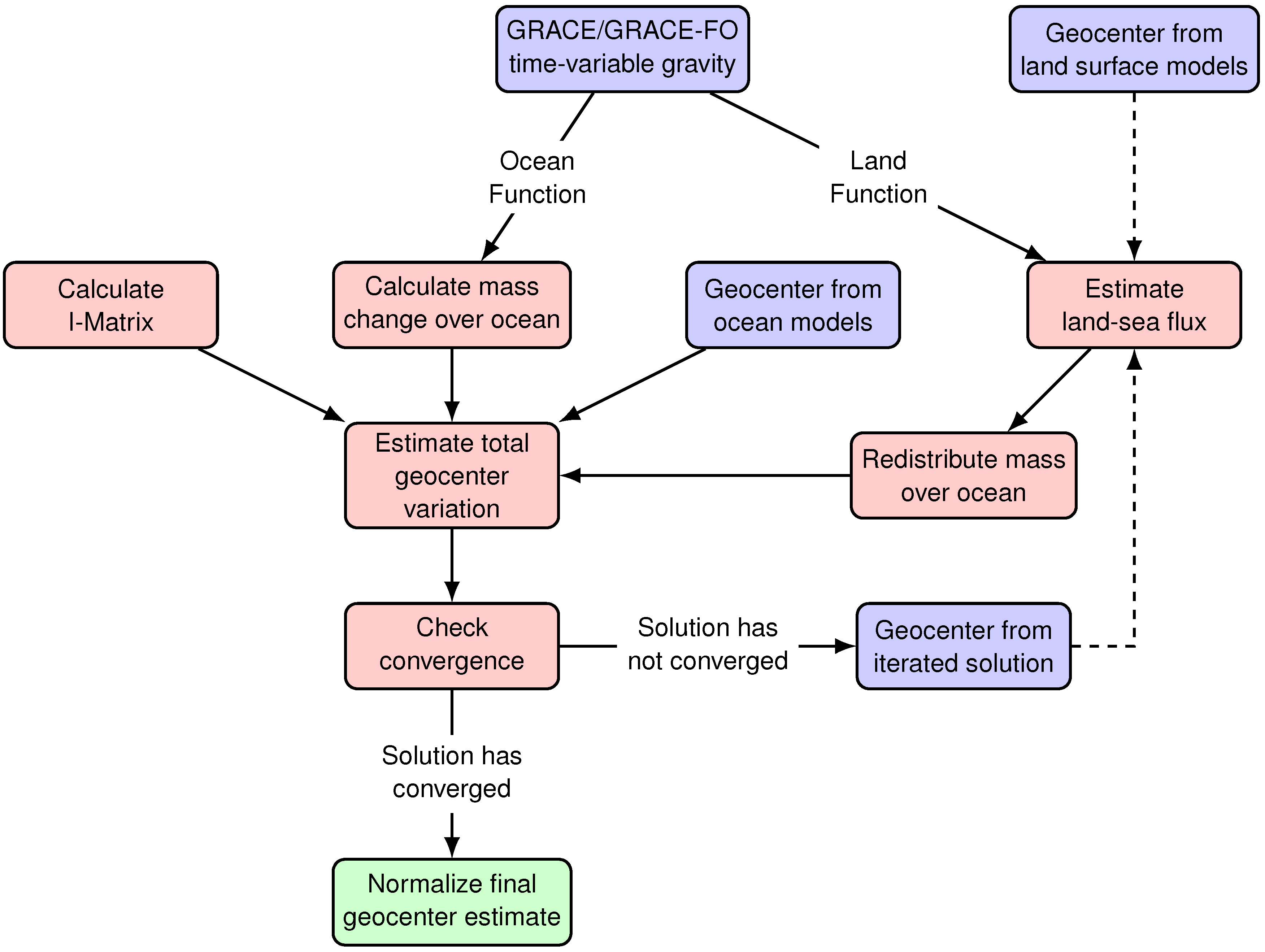
In order to estimate the full component of land-sea mass transport, an initial estimate of the geocenter variability is needed to calculate the total land mass [2]. Initially, we use annual and semi-annual geocenter estimates from Chen et al. [7], which are calculated from land-surface model estimates of soil moisture and snow water equivalent. We then calculate the eustatic sea level change induced from the land-sea flux and use it to generate a full geocenter estimate with Equation (9). The initial geocenter estimate from Chen et al. [7] is then replaced with the newly calculated estimate, and the sequence is repeated until the difference between successive iterations falls below a threshold value (see flowchart in Figure 2).
3.3. Spherical Harmonics of Atmospheric and Oceanic Variability
Changes in atmospheric pressure, p, and ocean bottom pressure, , at colatitude, , and longitude, , will impact the Earth’s gravitational field. These changes can be decomposed into a series of fully-normalized spherical harmonic coefficients representing the induced gravitational change after allowing for the Earth’s elastic response [49,50]:
The vertical integral, , in Equation (12) is determined based on assumptions of the Earth’s geometry and the vertical structure of the atmosphere or ocean [49].
Here, spherical harmonics from NCEP-DOE-2 and JRA-55 reanalyses are calculated assuming a thin layer two-dimensional atmosphere with a realistic Earth geometry incorporating the model orography, , and estimates of geoid height, (Equations (12) and (13)), while harmonics from ERA-Interim and MERRA-2 reanalyses are calculated assuming a three-dimensional atmospheric geometry integrating over the model layers (Equations (12) and (14)) [49].
Similarly, spherical harmonics from ECCO kf080i and ECCO V4r3 ocean bottom pressure are calculated assuming a thin layer two-dimensional ocean with a realistic Earth geometry incorporating estimates of geoid height and ocean bathymetry, (Equations (12) and (15)).
3.4. Time Series Analysis
We calculate the average geocenter change by simultaneously fitting a least-squares model with constant, linear and quadratic terms with annual, semiannual and 161-day oscillating terms to the estimate geocenter time series [51]. The 161-day oscillating terms account for aliasing of the S2 tidal constituent in the monthly GRACE/GRACE-FO time-variable gravity fields [52].
4. Results
4.1. Simulated Geocenter Estimates
We test the efficacy of our methodology for estimating geocenter variations by running experiments using fields of simulated global mass variability [2]. Sets of coefficients are constructed using estimates of terrestrial water storage (TWS) calculated from the Global Land Data Assimilation Systems (GLDAS) NOAH land surface model [53], estimates of surface mass balance (SMB) change for glaciers and ice caps calculated from the Regional Atmospheric and Climate Model (RACMO2.3) [54,55] and estimates of Greenland and Antarctic ice sheet mass balance from the mass budget method (MBM) [56]. Monthly GLDAS TWS estimates were calculated by combining the snow water equivalent, canopy water storage and soil moisture variables for non-glaciated regions [57]. We include the mass changes from glaciers and ice sheets to incorporate more processes that affect inter-annual geocenter variability [8]. The SMB of a glacier represents the sum of mass accumulation from snow and rain minus the surface ablation from meltwater runoff, sublimation, and snow drift erosion [58,59]. Cumulative anomalies in SMB were calculated for glaciers and ice caps in reference to a 1961–1990 baseline [60]. MBM estimates of ice sheet mass balance were calculated combining SMB outputs from RACMO2 with estimates of total ice discharge [56,61]. The sea level fingerprints of the synthetic data were calculated as an estimate of oceanic variability [48]. The ocean function used when calculating the sea level fingerprints in the synthetic is an update of Hall et al. [62] that incorporates Antarctic grounded ice delineations [63] and more accurate Greenland coastlines [64].
We test three different scenarios: (1) a uniform ocean redistribution of the land mass change with a static seasonal geocenter estimate similar to Swenson et al. [2], (2) a uniform ocean distribution of the land mass change that iteratively solves for the geocenter and (3) an oceanic redistribution taking into account self-attraction and loading effects that iteratively solves for the geocenter. Each model run uses spherical harmonic coefficients of degree two and greater that are calculated from the synthetic data. The harmonics are truncated to degree and order 60 and processed using the same 300 km Gaussian averaging function and decorrelation filter used with the GRACE/GRACE-FO data [4,29,30]. In order to calculate the full component of the land mass change, we include seasonal estimates of degree one variation from Chen et al. [7]. In the two iteration scenarios, we replace the degree one coefficients for each run with the calculated results of the previous run. The process is repeated until the difference between estimates on successive iterations falls below a threshold value.
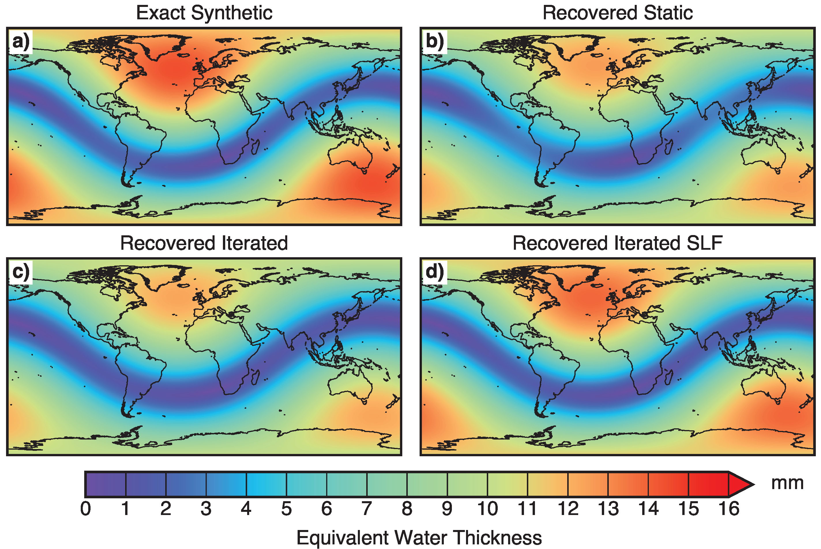
We compare the results of each scenario against the exact time series of degree one variations calculated from the synthetic dataset (Figure 3). The RMS differences between the scenarios and the original time series are 0.32 mm, 0.21 mm, and 0.11 mm for the static, iterated, and iterated SLF scenarios, respectively. This represents differences of 21%, 14%, and 7%, respectively, for each of the three scenarios compared to the standard deviation of the original time series. Calculating the land mass change using a static seasonal estimate of geocenter variability underestimates both the short-term and long-term variability in geocenter motion. Self-attraction and loading effects limit the recovery of geocenter variations in the two scenarios that assume a uniform redistribution of land-sea fluxes. The recovery of the seasonal variability of each coefficient is significantly improved when self-attraction and loading effects are incorporated (Figure 4).
4.2. Recovered Geocenter Estimates
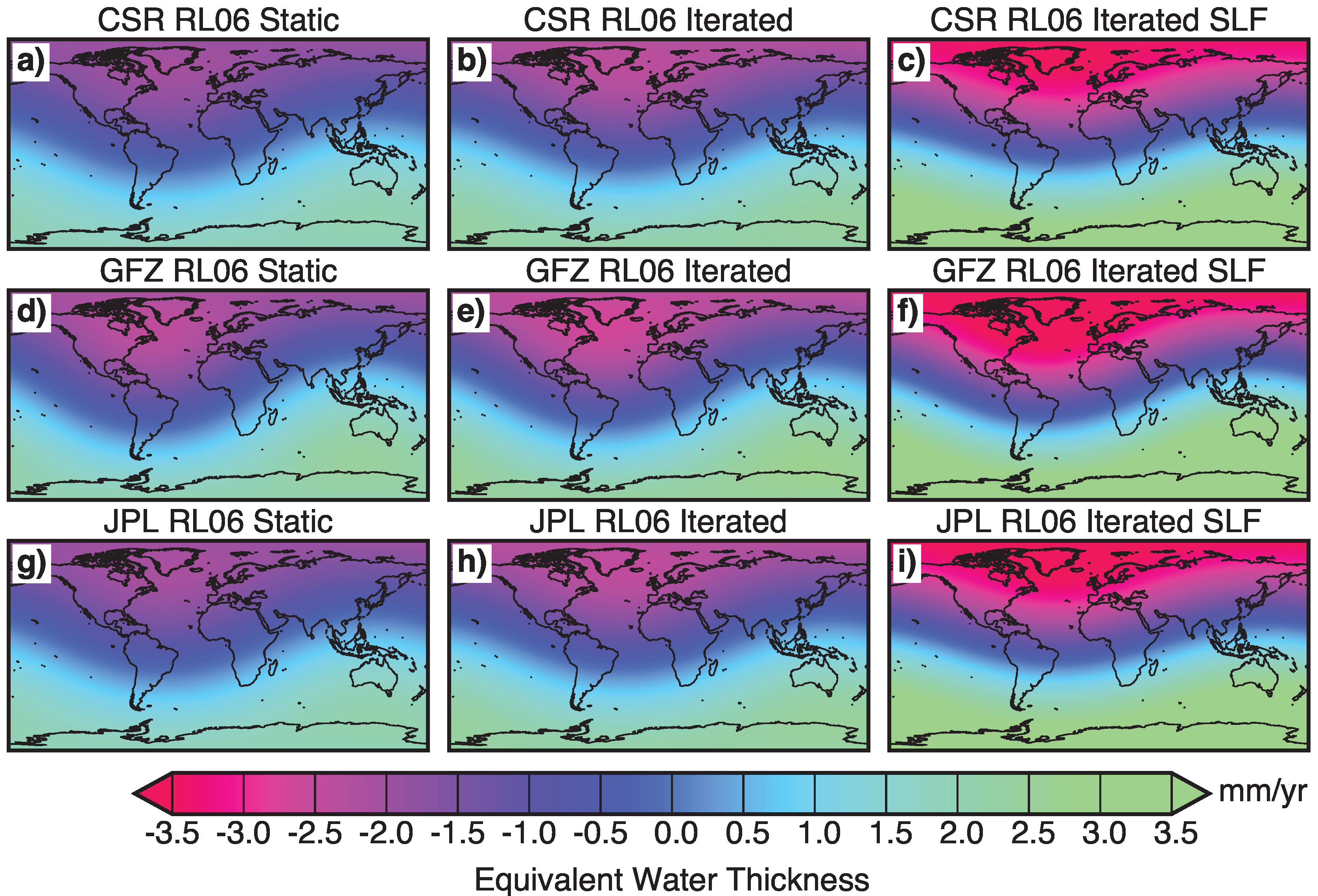
We estimate sets of degree one coefficients that are corrected for the effects of non-tidal atmospheric and oceanic variation [2]. These coefficients are directly applicable to time-variable gravity applications for estimating surface mass change [4]. We calculate geocenter variability estimates for each of the processing centers (CSR, GFZ, JPL) of the GRACE/GRACE-FO Science Data System (SDS) using the iterated self-consistent geocenter method that incorporates self-attraction and loading effects (Figure 5). Geocenter results from all three processing centers largely agree in terms of the amplitude and phase of the seasonal signal, along with the long-term trend in each coefficient. Self-attraction and loading effects impact the trend of the estimated geocenter solution for all three processing centers (Figure 6). Using a static seasonal geocenter to estimate the total land-sea flux results in weaker trends for all three processing centers. The trend and annual amplitudes of each coefficient calculated using time-variable gravity fields from each processing center are listed in Table 1. Annual amplitudes for solutions derived from satellite laser ranging (SLR) after correcting for non-tidal atmospheric and oceanic variability are listed for comparison [5,15]. The listed uncertainties for each coefficient are 95% confidence intervals, but do not take into account spherical harmonic errors or uncertainties in the geophysical corrections.
4.3. Uncertainty Estimates
The total uncertainty in the estimated geocenter time series represents a combination of GRACE/GRACE-FO measurement error, signal leakage between ocean and land, and uncertainty in the geophysical corrections. We assess the impact of these uncertainties, which we assume are uncorrelated, on the trend, annual amplitude and annual phase to the 95% confidence level. Monthly errors in the GRACE.GRACE-FO Level-2 spherical harmonics are estimated by first smoothing each coefficient with a 13-month Loess-type algorithm [13] and then calculating the residuals between the original and smoothed coefficients [65]. Spherical harmonic uncertainties contribute 0.11, 0.09 and 0.19 mm to the x, y, and z components for coefficients derived from CSR time-variable gravity fields.
We estimate the contribution from uncertainty in ocean circulation using ocean bottom pressure outputs from ECCO-JPL near real-time Kalman-filtered simulations and ECCO V4r3 simulations [36,38]. The time series of recovered degree one coefficients derived from CSR time-variable gravity fields using ocean bottom pressure outputs from ECCO-JPL kf080i [36], ECCO V4r3 [38] and MPIOM [23] are shown in Figure 7. The trend and annual amplitudes of each coefficient derived using the different ocean bottom pressure estimates are listed in Table 2. Solutions from ECCO-JPL agree with ECCO V4r3 and MPIOM derived solutions for the y and z components, but differs in terms of trend in the x-component [2]. Solutions from ECCO V4r3 and MPIOM agree for all coefficients between 2002 and 2014.
We estimate the uncertainty in atmospheric circulation by using an ensemble of reanalysis outputs [32,33,34,35]. Differences between the GRACE/GRACE-FO atmospheric de-aliasing product (GAA) and outputs from ERA-Interim [32], MERRA-2 [33], NCEP-DOE-2 [34], and JRA-55 [35] reanalyses will affect the estimates of geocenter motion. The average monthly uncertainty in geocenter variation due to uncertainties in atmospheric circulation is 0.07, 0.10, and 0.24 mm for the x, y, and z components, respectively.
Glacial Isostatic Adjustment (GIA) affects both ocean mass and land-sea flux calculations used to reconstruct the geocenter variation. The contribution of GIA uncertainty is calculated by comparing our best case estimate against the expected GIA rate from Caron et al. [26]. Using coefficients from Caron et al. [26] affects trend estimates by 0.04, 0.003, and 0.20 mm/yr for the x, y, and z components, respectively. This represents trend differences in the x, y, and z components of 21%, 3%, and 28%, respectively, compared with the values derived using GIA outputs from A et al. [25] with ICE-6G ice history. Uncertainty in GIA is a limiting factor for determining rates of geocenter change from reconstructions with time-variable gravity and ocean models.
5. Discussion
There is better agreement between the estimates derived from GRACE/GRACE-FO and the new CF-CM SLR-derived solutions compared with SLR-derived CN-CM estimates Figure 8, Table 1 [5]. Self-attraction and loading effects improve the correspondence with SLR-derived solutions, particularly in terms of average annual amplitude (Figure 9). However, there are still differences in the seasonal amplitudes of the z-component of geocenter motion (). Using a different ocean model to derive the oceanic component of geocenter variability cannot fully explain the difference between the solutions (Figure 8). Uncertainties in the GRACE spherical harmonics and uncertainties in atmospheric variation can partially explain the differences in the solutions. In addition, uncertainties in the ability to correct for network-effects in the SLR-derived CF-CM solutions can also help explain some discrepancies with the solutions derived from GRACE/GRACE-FO.
There is strong agreement between the three processing centers for each of the degree one coefficients during both the GRACE and GRACE-FO periods. However, between the end of 2015 and the end of the GRACE mission, there is disagreement between centers in estimates of the x and y components of geocenter motion ( and ). Operational procedures enacted to maintain the battery life of the GRACE satellites during the latter stages of the mission affected the quality of the time-variable gravity fields. The accelerometer onboard GRACE-B was turned off in September 2016 to reduce the battery load and maintain the operation of the microwave ranging instrument. Independent methods have been developed by the GRACE processing centers to spatiotemporally transplant the accelerometer data retrieved from GRACE-A for GRACE-B [66]. The increased uncertainty in the gravitational fields likely affects our ability to estimate the geocenter variability, particularly for the months with a single operating accelerometer.
Swenson et al. [2] provides a method for deriving geocenter motion from time-variable gravity measurements and estimates of ocean bottom pressure. The full component of oceanic mass is estimated in Swenson et al. [2] by calculating the land-sea fluxes using time-variable gravity measurements. We expand upon this method by using an iterated, self-consistent geocenter when calculating the full component of the land mass change, and by including self-attraction and loading effects when redistributing the mass over the ocean. The necessity of these inclusions only became evident with a longer record of time-variable gravity measurements. Using a static, seasonal geocenter omits the contribution of inter-annual fluctuations in degree one to the total land mass change. Self-attraction and loading effects impact both the seasonal amplitudes and the long-term trend of the recovered geocenter estimate (Figure 6 and Figure 9). This is due to the spatial patterns of sea level fingerprints that can deviate strongly from the uniform average, particularly over the long-term from changes in glaciers and ice sheets [48,67].
Sun et al. [16] expanded on Swenson et al. [2] by simultaneously estimating oblateness, , variations along with geocenter variations. They test the sensitivity of geocenter estimation methods to geophysical processes, such as glacial isostatic adjustment and ocean redistributions due to self-attraction and loading. In Sun et al. [16] the GRACE spherical harmonics are truncated to degree and order 45 and not processed with a decorrelation filter. Here, we use the full expansion of spherical harmonics for each processing center and filter for correlated errors in the GRACE/GRACE-FO harmonics [30]. The test the efficacy of the two methods using our synthetic reconstruction of global mass change. While statistically similar between the two techniques, we find that expanding to higher degree and orders and filtering produces more consistent estimates compared with synthetic estimate. The Sun et al. [16] method is used when calculating the JPL Tellus geocenter product. The differences between the geocenter estimates computed here and the estimates provided by JPL Tellus are largely during the final months of the GRACE mission and initial months of the GRACE-FO mission. Estimates of Antarctic ice sheet mass balance from time-variable gravity are sensitive to uncertainties in geocenter variation [68]. We find that differences between the two geocenter estimates affect Antarctic ice sheet mass balance estimates by 8–10 Gt/yr between 2002 and 2019.
Here, we use a buffered 300 km ocean function to calculate the sea level fingerprints in order to conserve mass and to reduce the leakage between land and ocean [4]. A full-resolution ocean function with realistic coastlines could be used if sets of scaling factors could be derived for both the land and ocean mass change. Typically, the use of scaling factors is applicable only for deriving seasonal fluctuations in land mass [69]. A more-complete scaling factor, such as from Hsu and Velicogna [67] for the land mass change, could possibly improve estimates of geocenter variation. The effects of self-attraction and loading would likely become more evident with a full-resolution ocean function as the effects can be more pronounced in coastal areas [48].
6. Conclusions
Geocenter variations are an important representation of global mass change, with applications in satellite gravimetry and in satellite orbit determination. Here, we investigate the effects of different calculations of the eustatic sea level caused by changes in land mass for estimating geocenter variations from combinations of ocean model outputs and time-variable gravity measurements from the GRACE and GRACE Follow-On missions. We find that using an iterated, self-consistent geocenter incorporating self-attraction and loading effects provides the best estimate of geocenter variation. Uncertainties from glacial isostatic adjustment, ocean circulation and atmospheric circulation limit the determination of geocenter position from this technique. The annual amplitudes of the z-component of geocenter variation differs between estimates from this technique and estimates derived from satellite laser ranging (SLR). The effects of self-attraction and loading improve the correspondence with SLR-derived coefficients but there are still discrepancies worth further investigation. Estimates of geocenter variations using data from the GRACE Follow-On mission are consistent with estimates from the GRACE mission, which enables the extension of the geocenter time series going forward.
Author Contributions
T.C.S. performed the analysis and wrote the manuscript. I.V. supervised the project, contributed to the analysis, helped analyze the data and provided comments/feedback.
Funding
Research was supported by an appointment to the NASA Postdoctoral Program at NASA Goddard Space Flight Center, administered by Universities Space Research Association under contract with NASA.
Acknowledgments
This work was performed at NASA Goddard Space Flight Center, the Jet Propulsion Laboratory, and University of California, Irvine. The authors thank our editor Thomas Gruber, and four anonymous reviewers for their comments and suggestions on improving this manuscript. The authors would like to thank John Ries (UTCSR) for his work to produce the geocenter solutions from satellite laser ranging (SLR) and for his helpful discussions on geocenter variability. The authors wish to thank Byron Tapley, Frank Flechtner, Michael Watkins, Srinivas Bettadpur and the GRACE/GRACE-FO Science Data System (SDS) teams for their work to produce the GRACE and GRACE-FO gravity solutions. The authors also wish to thank the German Space Operations Center (GSOC) of the German Aerospace Center (DLR) for providing the raw GRACE and GRACE-FO telemetry data to the processing centers. GRACE and GRACE-FO data are available from the NASA Physical Oceanography Distributed Active Archive Center (PO.DAAC) at https://podaac.jpl.nasa.gov/grace and the GFZ Information System and Data Center (ISDC) at http://isdc.gfz-potsdam.de/grace-isdc/. Reanalysis outputs are available from ERA-Interim at https://www.ecmwf.int/en/forecasts/datasets/reanalysis-datasets/era-interim, from MERRA-2 at https://gmao.gsfc.nasa.gov/reanalysis/MERRA-2/, from NCEP-DOE-2 at https://rda.ucar.edu/datasets/ds091.0/, and from JRA-55 at http://jra.kishou.go.jp/JRA-55/index_en.html. Documentation for the JPL Tellus ocean bottom pressure product is available at https://grace.jpl.nasa.gov/data/get-data/ocean-bottom-pressure/. Geocenter data from this project are available on Figshare under a CC BY 4.0 license at https://0-doi-org.brum.beds.ac.uk/10.6084/m9.figshare.7388540. The following programs are provided by this project for processing the GRACE/GRACE-FO data: https://github.com/tsutterley/read-GRACE-harmonics reads the Level-2 spherical harmonic data, and https://github.com/tsutterley/read-GRACE-geocenter reads the geocenter data provided by this project.
Conflicts of Interest
The authors declare no conflict of interest.
References
- Dong, D.; Dickey, J.O.; Chao, Y.; Cheng, M.K. Geocenter variations caused by atmosphere, ocean and surface ground water. Geophys. Res. Lett. 1997, 24, 1867–1870. [Google Scholar] [CrossRef]
- Swenson, S.C.; Chambers, D.P.; Wahr, J. Estimating geocenter variations from a combination of GRACE and ocean model output. J. Geophys. Res. Solid Earth 2008, 113, B08410. [Google Scholar] [CrossRef]
- Petit, G.; Luzum, B. IERS Conventions (2010); Technical Report 36, International Earth Rotation and Reference Systems Service (IERS); Verlag des Bundesamts für Kartographie und Geodäsie: Frankfurt am Main, Germany, 2010. [Google Scholar]
- Wahr, J.; Molenaar, M.; Bryan, F. Time variability of the Earth’s gravity field: Hydrological and oceanic effects and their possible detection using GRACE. J. Geophys. Res. Solid Earth 1998, 103, 30205–30229. [Google Scholar] [CrossRef]
- Ries, J. Reconciling Estimates of Annual Geocenter Motion from Space Geodesy. In Proceedings of the 20th International Workshop on Laser Ranging, Potsdam, Germany, 10–14 October 2016. [Google Scholar]
- Stolz, A. Changes in the Position of the Geocentre due to Seasonal Variations in Air Mass and Ground Water. Geophys. J. Int. 1976, 44, 19–26. [Google Scholar] [CrossRef] [Green Version]
- Chen, J.L.; Wilson, C.R.; Eanes, R.J.; Nerem, R.S. Geophysical interpretation of observed geocenter variations. J. Geophys. Res. Solid Earth 1999, 104, 2683–2690. [Google Scholar] [CrossRef]
- Wu, X.; Ray, J.; van Dam, T.M. Geocenter motion and its geodetic and geophysical implications. J. Geodyn. 2012, 58, 44–61. [Google Scholar] [CrossRef]
- Bettadpur, S. UTCSR Level-2 Processing Standards Document; Technical Report GRACE 327-742; Center for Space Research, University of Texas: Austin, TX, USA, 2018. [Google Scholar]
- Dahle, C.; Flechtner, F.; Murböck, M.; Michalak, G.; Neumayer, H.; Abrykosov, O.; Reinhold, A.; König, R. GFZ Processing Standards Document for Level-2 Product Release 06; Technical Report GRACE 327-743; GFZ German Research Centre for Geosciences: Potsdam, Germany, 2018. [Google Scholar]
- Yuan, D.N. JPL Level-2 Processing Standards Document for Level-2 Product Release 06; Technical Report GRACE 327-744; Jet Propulsion Laboratory: Pasadena, CA, USA, 2018. [Google Scholar]
- Chambers, D.P.; Wahr, J.; Nerem, R.S. Preliminary observations of global ocean mass variations with GRACE. Geophys. Res. Lett. 2004, 31, L13310. [Google Scholar] [CrossRef]
- Velicogna, I. Increasing rates of ice mass loss from the Greenland and Antarctic ice sheets revealed by GRACE. Geophys. Res. Lett. 2009, 36, L19503. [Google Scholar] [CrossRef]
- Chen, J.L.; Rodell, M.; Wilson, C.R.; Famiglietti, J.S. Low degree spherical harmonic influences on Gravity Recovery and Climate Experiment (GRACE) water storage estimates. Geophys. Res. Lett. 2005, 32, L14405. [Google Scholar] [CrossRef]
- Cheng, M.K. Geocenter Variations from Analysis of SLR Data; Reference Frames for Applications in Geosciences; Springer: Berlin/Heidelberg, Germany, 2013; pp. 19–25. [Google Scholar] [CrossRef]
- Sun, Y.; Riva, R.; Ditmar, P. Optimizing estimates of annual variations and trends in geocenter motion and J2 from a combination of GRACE data and geophysical models. J. Geophys. Res. Solid Earth 2016, 121, 8352–8370. [Google Scholar] [CrossRef]
- Rietbroek, R.; Fritsche, M.; Brunnabend, S.E.; Daras, I.; Kusche, J.; Schröter, J.; Flechtner, F.M.; Dietrich, R. Global surface mass from a new combination of GRACE, modelled OBP and reprocessed GPS data. J. Geodyn. 2012, 59–60, 64–71. [Google Scholar] [CrossRef]
- Wu, X.; Heflin, M.B.; Schotman, H.; Vermeersen, B.L.A.; Dong, D.; Gross, R.S.; Ivins, E.R.; Moore, A.W.; Owen, S.E. Simultaneous estimation of global present-day water transport and glacial isostatic adjustment. Nat. Geosci. 2010, 3, 642–646. [Google Scholar] [CrossRef]
- Collilieux, X.; Altamimi, Z.; Ray, J.; van Dam, T.M.; Wu, X. Effect of the satellite laser ranging network distribution on geocenter motion estimation. J. Geophys. Res. Solid Earth 2009, 114, B04402. [Google Scholar] [CrossRef]
- Zannat, U.J.; Tregoning, P. Estimating network effect in geocenter motion: Theory. J. Geophys. Res. Solid Earth 2017, 122, 8360–8375. [Google Scholar] [CrossRef]
- Tapley, B.D. GRACE Measurements of Mass Variability in the Earth System. Science 2004, 305, 503–505. [Google Scholar] [CrossRef] [PubMed] [Green Version]
- Loomis, B.D.; Rachlin, K.E.; Luthcke, S.B. Improved Earth Oblateness Rate Reveals Increased Ice Sheet Losses and Mass-Driven Sea Level Rise. Geophys. Res. Lett. 2019, 46, 6910–6917. [Google Scholar] [CrossRef]
- Flechtner, F.; Dobslaw, H.; Fagiolini, E. AOD1B Product Description Document for Product Release 05; Technical Report GRACE 327-750; GFZ German Research Centre for Geosciences: Potsdam, Germany, 2015. [Google Scholar]
- Dobslaw, H.; Bergmann-Wolf, I.; Dill, R.; Poropat, L.; Thomas, M.; Dahle, C.; Esselborn, S.; König, R.; Flechtner, F. A new high-resolution model of non-tidal atmosphere and ocean mass variability for de-aliasing of satellite gravity observations: AOD1B RL06. Geophys. J. Int. 2017, 211, 263–269. [Google Scholar] [CrossRef] [Green Version]
- Geruo, A.; Wahr, J.; Zhong, S. Computations of the viscoelastic response of a 3-D compressible Earth to surface loading: An application to Glacial Isostatic Adjustment in Antarctica and Canada. Geophys. J. Int. 2013, 192, 557–572. [Google Scholar] [CrossRef]
- Caron, L.; Ivins, E.R.; Larour, E.; Adhikari, S.; Nilsson, J.; Blewitt, G. GIA Model Statistics for GRACE Hydrology, Cryosphere, and Ocean Science. Geophys. Res. Lett. 2018, 45, 2203–2212. [Google Scholar] [CrossRef]
- Wahr, J.; DaZhong, H.; Trupin, A.S. Predictions of vertical uplift caused by changing polar ice volumes on a viscoelastic Earth. Geophys. Res. Lett. 1995, 22, 977–980. [Google Scholar] [CrossRef]
- Trupin, A.S.; Meier, M.F.; Wahr, J. Effect of melting glaciers on the Earth’s rotation and gravitational field: 1965–1984. Geophys. J. Int. 1992, 108, 1–15. [Google Scholar] [CrossRef]
- Jekeli, C. Alternative Methods to Smooth the Earth’s Gravity Field; Technical Report 327; Ohio State University, Department of Geodetic Science and Surveying, 1958 Neil Avenue: Columbus, OH, USA, 1981. [Google Scholar]
- Swenson, S.C.; Wahr, J. Post-processing removal of correlated errors in GRACE data. Geophys. Res. Lett. 2006, 33, L08402. [Google Scholar] [CrossRef]
- Cheng, M. Geocenter Variations from Analysis of TOPEX/Poseidon SLR Data; Technical Report 25; International Earth Rotation and Reference Systems Service (IERS): Frankfurt am Main, Germany, 1998. [Google Scholar]
- Berrisford, P.; Dee, D.P.; Poli, P.; Brugge, R.; Fielding, K.; Fuentes, M.; Kållberg, P.W.; Kobayashi, S.; Uppala, S.; Simmons, A. The ERA-Interim Archive Version 2.0; ERA Report Series; ECMWF: Reading, UK, 2011; p. 23. [Google Scholar]
- Bosilovich, M.G.; Lucchesi, R.; Suarez, M. MERRA-2: File Specification. GMAO Office Note 2016, 9, 1–73. [Google Scholar]
- Kanamitsu, M.; Ebisuzaki, W.; Woollen, J.; Yang, S.K.; Hnilo, J.J.; Fiorino, M.; Potter, G.L. NCEP–DOE AMIP-II Reanalysis (R-2). Bull. Am. Meteorol. Soc. 2002, 83, 1631–1644. [Google Scholar] [CrossRef]
- Kobayashi, S.; Ota, Y.; Harada, Y.; Ebita, A.; Moriya, M.; Onoda, H.; Onogi, K.; Kamahori, H.; Kobayashi, C.; Endo, H.; et al. The JRA-55 Reanalysis: General Specifications and Basic Characteristics. J. Meteorol. Soc. Jpn. Ser. II 2015, 93, 5–48. [Google Scholar] [CrossRef] [Green Version]
- Fukumori, I. A Partitioned Kalman Filter and Smoother. Mon. Weather Rev. 2002, 130, 1370–1383. [Google Scholar] [CrossRef]
- Kim, S.B.; Lee, T.; Fukumori, I. Mechanisms Controlling the Interannual Variation of Mixed Layer Temperature Averaged over the Niño-3 Region. J. Clim. 2007, 20, 3822–3843. [Google Scholar] [CrossRef]
- Fukumori, I.; Wang, O.; Fenty, I.; Forget, G.; Heimbach, P.; Ponte, R.M. ECCO Version 4 Release 3; Technical report; JPL/Caltech and NASA Physical Oceanography: Pasadena, CA, USA, 2017. [Google Scholar]
- Forget, G.; Campin, J.M.; Heimbach, P.; Hill, C.N.; Ponte, R.M.; Wunsch, C. ECCO version 4: An integrated framework for non-linear inverse modeling and global ocean state estimation. Geosci. Model Dev. 2015, 8, 3071–3104. [Google Scholar] [CrossRef]
- Forget, G.; Ponte, R.M. The partition of regional sea level variability. Prog. Oceanogr. 2015, 137, 173–195. [Google Scholar] [CrossRef] [Green Version]
- Losch, M.; Menemenlis, D.; Campin, J.M.; Heimbach, P.; Hill, C. On the formulation of sea-ice models. Part 1: Effects of different solver implementations and parameterizations. Ocean Model. 2010, 33, 129–144. [Google Scholar] [CrossRef] [Green Version]
- Greatbatch, R.J. A note on the representation of steric sea level in models that conserve volume rather than mass. J. Geophys. Res. Oceans 1994, 99, 12767–12771. [Google Scholar] [CrossRef]
- Farrell, W.E.; Clark, J.A. On Postglacial Sea Level. Geophys. J. R. Astron. Soc. 1976, 46, 647–667. [Google Scholar] [CrossRef]
- Clark, J.A.; Lingle, C.S. Future sea-level changes due to West Antarctic ice sheet fluctuations. Nature 1977, 269, 206–209. [Google Scholar] [CrossRef]
- Mitrovica, J.X.; Milne, G.A. On post-glacial sea level: I. General theory. Geophys. J. Int. 2003, 154, 253–267. [Google Scholar] [CrossRef] [Green Version]
- Tamisiea, M.E.; Mitrovica, J.X. The Moving Boundaries of Sea Level Change: Understanding the Origins of Geographic Variability. Oceanography 2011, 24, 24–39. [Google Scholar] [CrossRef]
- Kendall, R.A.; Mitrovica, J.X.; Milne, G.A. On post-glacial sea level – II. Numerical formulation and comparative results on spherically symmetric models. Geophys. J. Int. 2005, 161, 679–706. [Google Scholar] [CrossRef]
- Tamisiea, M.E.; Hill, E.M.; Ponte, R.M.; Davis, J.L.; Velicogna, I.; Vinogradova, N.T. Impact of self-attraction and loading on the annual cycle in sea level. J. Geophys. Res. Oceans 2010, 115, C07004. [Google Scholar] [CrossRef]
- Boy, J.P.; Chao, B.F. Precise evaluation of atmospheric loading effects on Earth’s time-variable gravity field. J. Geophys. Res. Solid Earth 2005, 110, B08412. [Google Scholar] [CrossRef]
- Swenson, S.; Wahr, J. Estimated effects of the vertical structure of atmospheric mass on the time-variable geoid. J. Geophys. Res. Solid Earth 2002, 107, 2194. [Google Scholar] [CrossRef]
- Velicogna, I.; Sutterley, T.C.; van den Broeke, M.R. Regional acceleration in ice mass loss from Greenland and Antarctica using GRACE time-variable gravity data. Geophys. Res. Lett. 2014, 41, 8130–8137. [Google Scholar] [CrossRef] [Green Version]
- Chen, J.L.; Wilson, C.R.; Seo, K.W. S2 tide aliasing in GRACE time-variable gravity solutions. J. Geod. 2009, 83, 679–687. [Google Scholar] [CrossRef]
- Rodell, M.; Houser, P.R.; Jambor, U.; Gottschalck, J.; Mitchell, K.; Meng, C.J.; Arsenault, K.; Cosgrove, B.; Radakovich, J.; Bosilovich, M.; et al. The Global Land Data Assimilation System. Bull. Am. Meteorol. Soc. 2004, 85, 381–394. [Google Scholar] [CrossRef] [Green Version]
- Noël, B.; van de Berg, W.J.; Lhermitte, S.; Wouters, B.; Schaffer, N.; van den Broeke, M.R. Six decades of glacial mass loss in the Canadian Arctic Archipelago. J. Geophys. Res. Earth Surf. 2018, 123, 1430–1449. [Google Scholar] [CrossRef]
- Noël, B.; van de Berg, W.J.; van Wessem, J.M.; van Meijgaard, E.; van As, D.; Lenaerts, J.T.M.; Lhermitte, S.; Kuipers Munneke, P.; Smeets, C.J.P.P.; van Ulft, L.H.; et al. Modelling the climate and surface mass balance of polar ice sheets using RACMO2 – Part 1: Greenland (1958–2016). Cryosphere 2018, 12, 811–831. [Google Scholar] [CrossRef]
- Rignot, E.J.; Velicogna, I.; van den Broeke, M.R.; Monaghan, A.J.; Lenaerts, J.T.M. Acceleration of the contribution of the Greenland and Antarctic ice sheets to sea level rise. Geophys. Res. Lett. 2011, 38, L05503. [Google Scholar] [CrossRef]
- Syed, T.H.; Famiglietti, J.S.; Rodell, M.; Chen, J.; Wilson, C.R. Analysis of terrestrial water storage changes from GRACE and GLDAS. Water Resour. Res. 2008, 44. [Google Scholar] [CrossRef]
- Ettema, J.; van den Broeke, M.R.; van Meijgaard, E.; van de Berg, W.J.; Bamber, J.L.; Box, J.E.; Bales, R.C. Higher surface mass balance of the Greenland ice sheet revealed by high-resolution climate modeling. Geophys. Res. Lett. 2009, 36, L12501. [Google Scholar] [CrossRef]
- Lenaerts, J.T.M.; van den Broeke, M.R.; van de Berg, W.J.; van Meijgaard, E.; Kuipers Munneke, P. A new, high-resolution surface mass balance map of Antarctica (1979–2010) based on regional atmospheric climate modeling. Geophys. Res. Lett. 2012, 39, L04501. [Google Scholar] [CrossRef]
- Van den Broeke, M.R.; Bamber, J.L.; Ettema, J.; Rignot, E.J.; Schrama, E.; van de Berg, W.J.; van Meijgaard, E.; Velicogna, I.; Wouters, B. Partitioning Recent Greenland Mass Loss. Science 2009, 326, 984–986. [Google Scholar] [CrossRef] [Green Version]
- Rignot, E.J.; Bamber, J.L.; van den Broeke, M.R.; Davis, C.H.; Li, Y.; van de Berg, W.J.; van Meijgaard, E. Recent Antarctic ice mass loss from radar interferometry and regional climate modelling. Nat. Geosci. 2008, 1, 106–110. [Google Scholar] [CrossRef] [Green Version]
- Hall, F.G.; Brown de Colstoun, E.; Collatz, G.J.; Landis, D.; Dirmeyer, P.; Betts, A.; Huffman, G.J.; Bounoua, L.; Meeson, B. ISLSCP Initiative II global data sets: Surface boundary conditions and atmospheric forcings for land-atmosphere studies. J. Geophys. Res. Atmos. 2006, 111. [Google Scholar] [CrossRef]
- Mouginot, J.; Scheuchl, B.; Rignot, E. MEaSUREs Antarctic Boundaries for IPY 2007–2009 from Satellite Radar; Version 2; NASA National Snow and Ice Data Center Distributed Active Archive Center: Boulder, CO, USA, 2017. [Google Scholar] [CrossRef]
- Henriksen, N.; Higgins, A.; Kalsbeek, F.; Pulvertaft, T.C.R. Greenland from Archaean to Quaternary, Descriptive text to the 1995 Geological Map of Greenland 1:2,500,000. Geol. Surv. Den. Greenl. Bull. 2009, 18, 1–126. [Google Scholar]
- Wahr, J.; Swenson, S.C.; Velicogna, I. Accuracy of GRACE mass estimates. Geophys. Res. Lett. 2006, 33, L06401. [Google Scholar] [CrossRef]
- Bandikova, T.; McCullough, C.; Kruizinga, G.L.; Save, H.; Christophe, B. GRACE accelerometer data transplant. Adv. Space Res. 2019, 64, 623–644. [Google Scholar] [CrossRef] [Green Version]
- Hsu, C.W.; Velicogna, I. Detection of Sea Level Fingerprints derived from GRACE gravity data. Geophys. Res. Lett. 2017, 2017GL074070. [Google Scholar] [CrossRef]
- Velicogna, I.; Wahr, J. Time-variable gravity observations of ice sheet mass balance: Precision and limitations of the GRACE satellite data. Geophys. Res. Lett. 2013, 40, 3055–3063. [Google Scholar] [CrossRef] [Green Version]
- Landerer, F.W.; Swenson, S.C. Accuracy of scaled GRACE terrestrial water storage estimates. Water Resour. Res. 2012, 48. [Google Scholar] [CrossRef]
Figure 1.
Schematic of the major geophysical processes contributing to mass variability sensed by time-variable gravity.
Figure 1.
Schematic of the major geophysical processes contributing to mass variability sensed by time-variable gravity.

Figure 2.
Flowchart of our processing scheme for estimating geocenter variations from time-variable gravity data and ocean model outputs. Blue nodes denote datasets, red nodes denote calculations, and the green node denotes the final converged solution.
Figure 2.
Flowchart of our processing scheme for estimating geocenter variations from time-variable gravity data and ocean model outputs. Blue nodes denote datasets, red nodes denote calculations, and the green node denotes the final converged solution.

Figure 3.
Time series of actual and recovered geocenter variations, (a) x, (b) y and (c) z, in mm from synthetic fields of mass variability derived from GLDAS NOAH v2.1 land surface model outputs [53], RACMO2.3 surface mass balance outputs [54,55] and ice sheet mass balance estimates [56]. The gray line is the original degree one time series calculated directly from the synthetic dataset. The orange, purple and green lines are the derived degree one time series using different scenarios to calculate the land-sea fluxes. The orange line uses a static seasonal geocenter from Chen et al. [7], the purple line uses an iterated self-consistent geocenter, and the green line uses an iterated self-consistent geocenter taking into account the effects of self-attraction and loading.

Figure 4.
Annual amplitudes of (a) actual and (b–d) recovered degree one surface mass variations in mm water equivalent calculated from synthetic fields of mass variability derived from GLDAS NOAH v2.1 land surface model outputs [53], RACMO2.3 surface mass balance outputs [54,55] and ice sheet mass balance estimates [56]. In the recovered solutions, the land-sea exchange is estimated using (b) a static seasonal geocenter from Chen et al. [7], (c) an iterated self-consistent geocenter, and (d) an iterated self-consistent geocenter taking into account the effects of self-attraction and loading.

Figure 5.
Time series of recovered geocenter variations, (a) x, (b) y and (c) z, in mm calculated using an iterated self-consistent geocenter with self-attraction and loading effects from time-variable gravity fields provided by the Center for Space Research (orange), the German Research Centre for Geosciences (purple) and the Jet Propulsion Laboratory (green). The gray shading denotes the period between the GRACE and GRACE-FO missions.

Figure 6.
Trends in recovered degree one surface mass variations in mm water equivalent calculated from time-variable gravity fields provided by the Center for Space Research (a–c), the German Research Centre for Geosciences (d–f) and the Jet Propulsion Laboratory (g–i). The land-sea exchange is calculated in the first column (a,d,g) with a static seasonal geocenter from Chen et al. [7], in the second column (b,e,h) with an iterated self-consistent geocenter, and in the third column (c,f,i) with an iterated self-consistent geocenter taking into account the effects of self-attraction and loading.

Figure 7.
Time series of recovered geocenter variations, (a) x, (b) y and (c) z, in mm calculated using an iterated self-consistent geocenter with self-attraction and loading effects from time-variable gravity fields provided by the Center for Space Research using ocean bottom pressure outputs from ECCO-JPL real-time Kalman-filtered simulations (orange) [36], ECCO Version 4 Release 3 simulations (purple) [38], and Max Planck Institute ocean model (MPIOM) [24].

Figure 8.
Time series of measured and recovered geocenter variations, (a) x, (b) y and (c) z, in mm from satellite laser ranging (orange and purple) and time-variable gravity fields provided by the Center for Space Research (green). The SLR-derived solutions in orange (CN-CM) are the traditional solutions that center the SLR network [15], and the SLR-derived solutions in purple (CF-CM) include the effects of local site displacements [5]. The solutions derived from GRACE/GRACE-FO in green use an iterated self-consistent geocenter that takes into account the effects of self-attraction and loading.

Figure 9.
Annual amplitudes of measured and recovered degree one surface mass variations in mm water equivalent calculated from (a–c) time-variable gravity fields provided by the Center for Space Research, and (d) satellite laser ranging (SLR) CF-CM solutions. In the solutions derived from GRACE/GRACE-FO, the land-sea exchange is estimated using (a) a static seasonal geocenter from Chen et al. [7], (b) an iterated self-consistent geocenter, and (c) an iterated self-consistent geocenter taking into account the effects of self-attraction and loading.


Table 1.
Geocenter motion annual amplitudes, annual phase, and trends for 2002–2017 derived using satellite laser ranging (SLR) and time-variable gravity fields from the Center for Space Research (CSR), the German Research Centre for Geosciences (GFZ) and the Jet Propulsion Laboratory (JPL) corrected for the effects of non-tidal atmospheric and oceanic variation. Errors denote the 95% confidence level.
| x | y | z | ||||
|---|---|---|---|---|---|---|
| Annual Amplitude [mm] | ||||||
| CSR | 1.34 ± 0.11 | 1.54 ± 0.12 | 2.25 ± 0.16 | |||
| GFZ | 1.38 ± 0.14 | 1.56 ± 0.13 | 2.30 ± 0.16 | |||
| JPL | 1.31 ± 0.11 | 1.52 ± 0.12 | 2.20 ± 0.17 | |||
| SLR CN-CM | 1.93 ± 0.38 | 1.17 ± 0.38 | 4.25 ± 0.57 | |||
| SLR CF-CM | 1.29 ± 0.29 | 1.48 ± 0.23 | 2.97 ± 0.46 | |||
| Annual Phase [day] | ||||||
| CSR | 356.5 ± 5.0 | 151.9 ± 4.6 | 9.6 ± 4.2 | |||
| GFZ | 352.7 ± 5.7 | 150.7 ± 4.9 | 4.5 ± 4.1 | |||
| JPL | 355.0 ± 4.8 | 151.4 ± 4.7 | 7.9 ± 4.4 | |||
| SLR CN-CM | 5.5 ± 11.7 | 194.7 ± 18.9 | 52.4 ± 7.7 | |||
| SLR CF-CM | 347.9 ± 13.3 | 169.6 ± 9.0 | 46.3 ± 9.1 | |||
| Trend [mm/yr] | ||||||
| CSR | −0.15 ± 0.02 | 0.10 ± 0.02 | −0.62 ± 0.03 | |||
| GFZ | −0.19 ± 0.03 | 0.21 ± 0.03 | −0.66 ± 0.03 | |||
| JPL | −0.15 ± 0.02 | 0.11 ± 0.03 | −0.63 ± 0.03 | |||
Table 2.
Geocenter motion annual amplitudes, annual phase, and trends for 2002–2015 derived using time-variable gravity fields from the Center for Space Research (CSR) using ocean bottom pressure outputs from ECCO-JPL real-time Kalman-filtered simulations (kf080i) [36] and ECCO Version 4 Release 3 simulations (V4r3) [38]. Errors denote the 95% confidence level.
| x | y | z | ||||
|---|---|---|---|---|---|---|
| Annual Amplitude [mm] | ||||||
| ECCO-JPL kf080i | 1.46 ± 0.20 | 1.28 ± 0.17 | 1.80 ± 0.31 | |||
| ECCO V4r3 | 1.63 ± 0.18 | 1.21 ± 0.16 | 2.31 ± 0.27 | |||
| MPIOM | 1.34 ± 0.11 | 1.55 ± 0.13 | 2.24 ± 0.16 | |||
| Annual Phase [day] | ||||||
| ECCO-JPL kf080i | 307.3 ± 7.9 | 165.5 ± 7.9 | 327.8 ± 9.9 | |||
| ECCO V4r3 | 323.0 ± 6.5 | 150.8 ± 7.7 | 326.2 ± 6.9 | |||
| MPIOM | 358.3 ± 5.0 | 150.3 ± 4.8 | 9.6 ± 4.3 | |||
| Trend [mm/yr] | ||||||
| ECCO-JPL kf080i | −0.32 ± 0.04 | 0.16 ± 0.03 | −0.48 ± 0.06 | |||
| ECCO V4r3 | −0.10 ± 0.04 | 0.12 ± 0.04 | −0.44 ± 0.06 | |||
| MPIOM | −0.12 ± 0.02 | 0.08 ± 0.03 | −0.62 ± 0.03 | |||
© 2019 by the authors. Licensee MDPI, Basel, Switzerland. This article is an open access article distributed under the terms and conditions of the Creative Commons Attribution (CC BY) license (http://creativecommons.org/licenses/by/4.0/).
Share and Cite
MDPI and ACS Style
Sutterley, T.C.; Velicogna, I. Improved Estimates of Geocenter Variability from Time-Variable Gravity and Ocean Model Outputs. Remote Sens. 2019, 11, 2108. https://0-doi-org.brum.beds.ac.uk/10.3390/rs11182108
AMA Style
Sutterley TC, Velicogna I. Improved Estimates of Geocenter Variability from Time-Variable Gravity and Ocean Model Outputs. Remote Sensing. 2019; 11(18):2108. https://0-doi-org.brum.beds.ac.uk/10.3390/rs11182108
Chicago/Turabian StyleSutterley, Tyler C., and Isabella Velicogna. 2019. "Improved Estimates of Geocenter Variability from Time-Variable Gravity and Ocean Model Outputs" Remote Sensing 11, no. 18: 2108. https://0-doi-org.brum.beds.ac.uk/10.3390/rs11182108
Note that from the first issue of 2016, this journal uses article numbers instead of page numbers. See further details here.