1. Introduction
Every day moderate- to large-magnitude earthquakes occur, generating instantaneously coseismic ground deformations of the Earth’s crust, and Italy can be considered as one of the most tectonically active regions of the world [
1,
2,
3].
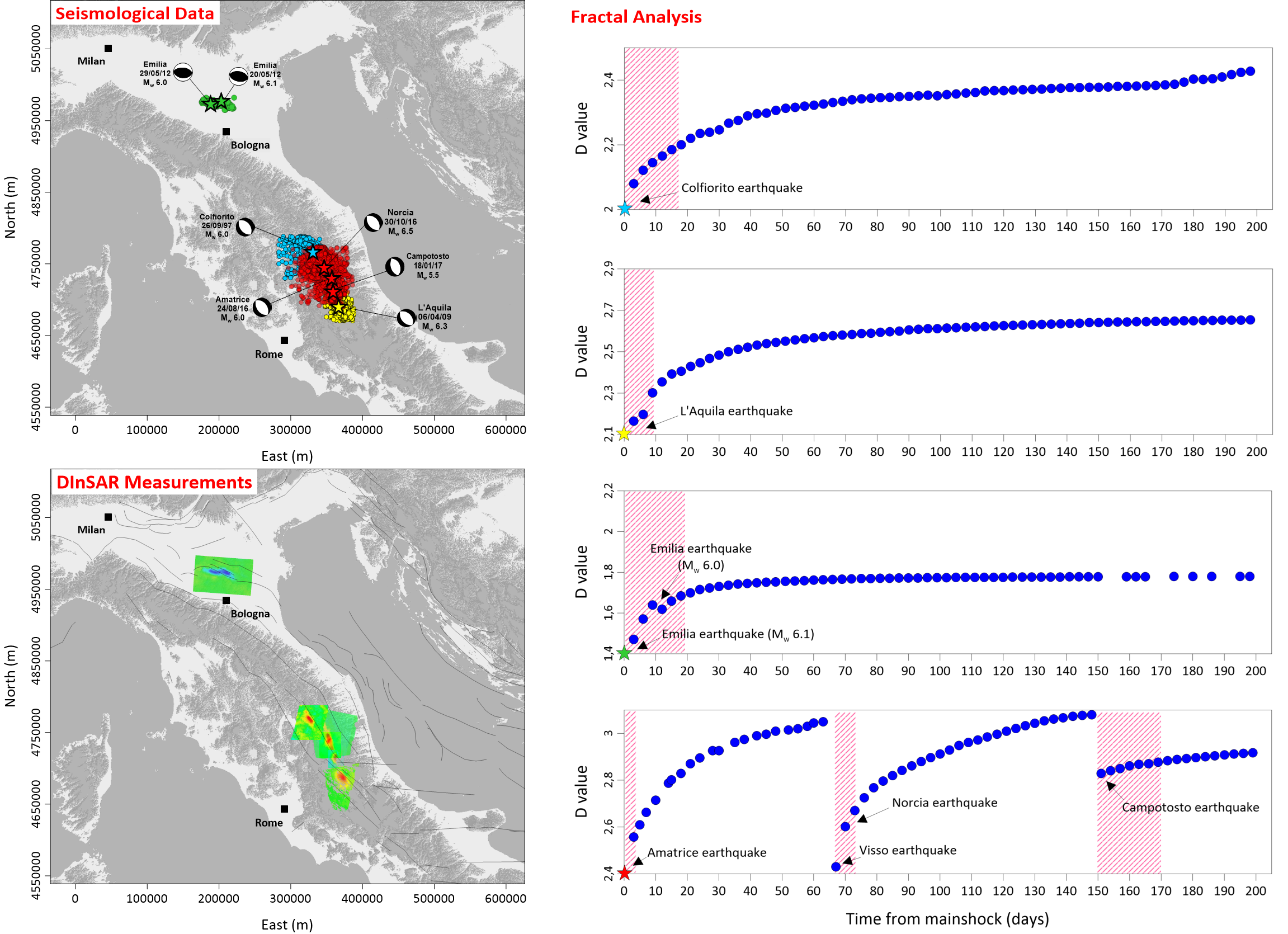
Figure 1 shows the distribution of historical and recent earthquakes [
4]; compressional focal mechanisms are prevalent at the fronts of the Alps and the Apennines, while extensional mechanisms dominate along the Apennines belt [
5].
The Italian peninsula extends for more than 1000 km within the central Mediterranean, forming a narrow (<200 km) mountain belt (
Figure 1a) between the European and African converging plates. Because of this convergence process and of the consequent subduction of the Adriatic-Ionian lithosphere, which has been active since the Cretaceous, two different orogens (i.e., the Alps and the Apennines) have developed [
6,
7]. These two mountain belts and, mainly, the Apennines, represent the locations of the current seismicity and of the most significant tectonic processes of the Italian peninsula. In particular, since at least Pliocene time, the central Apennines fold-and-thrust belt underwent extensional tectonics associated with the Tyrrhenian back-arc basin opening in the west; this extensional tectonics followed and replaced the previous compressional one which formed the accretionary prism, presently shifted to the east (western Adriatic Sea) [
8]. This extensional process generated a system of NW–SE-oriented normal faults, which dissected the fold-and-thrust belt [
9] and represent the seismogenic structures that generate, over the centuries, medium-high intensity earthquakes in the axial and western parts of the mountain belt (
Figure 1a) [
4,
10]. As documented by Global Positioning System (GPS) and borehole breakouts data and seismicity distribution, the main active process is the extension observable along the entire Apennines belt with a NE-SW orientation, up to the Calabria region where the extension directions rotate from NE-SW to NW-SE, following the curved shape of the Calabrian arc. On the other hand, compression is limited to the external areas, along the northern Apennines front, offshore along the northern Sicilian coast, and to the Po Plain and Friuli regions; present-day stress information confirms that there is no clear evidence of compression along the front of the central and southern Apennines. Strike-slip faulting is rare in Italy and spatially restricted to areas located along the southern Apennines foredeep and in eastern Sicily [
11,
12,
13].
Italian geodynamics expresses itself through seismic patterns that are peculiar when considering the known tectonic contexts. In fact, the seismicity in the Alps is mainly concentrated at the margins of the orogen, in areas of low elevation, although some relevant earthquakes are located also within the belt itself; the main focal mechanisms are compressional [
5]. Conversely, the Apennines chain is rather dominated by extensional seismicity along the main ridge of the belt, at 10–15 km depth; compressional mechanisms (thrust ramps or decollements) were recorded in the frontal Apennines to the east in the external, low-relief or marine areas of the accretionary prism [
10,
14,
15]. Moreover, local transfer zones are accommodated by strike–slip faults in all areas.
The stress map of Italy confirms the pattern shown by the seismicity: compression all around the Alps and at the submersed front of the Apennines, and extension along this belt, plus some strike–slip transfer zones, mainly located in areas where the advancement velocity of the thrust front changes abruptly [
13]. Extension can be observed along the Apennines axis and in the Tyrrhenian Sea, whereas compression occurs at the front of the Apennines accretionary prism, and along the front of the Alps. The stress pattern is also consistent with space geodesy data: GPS show intersites data with velocities up to about 5 mm/year, whereas strain rates are in the order of 10–40 nanostrains/year [
5,
16].
The increasing availability of data, such as those derived from Differential Synthetic Aperture Radar Interferometry (DInSAR) and seismology, allows us to study in detail the spatial and temporal evolution of a seismic sequence and its features. In this context, the study of an earthquake mechanism is usually completed by the determination of a fault plane and the direction of displacement along it. However, in order to study other characteristics of faulting processes, it can be relevant to apply the Fractals Theory and to analyze the fractal dimension temporal evolution [
17,
18,
19,
20,
21,
22,
23]. For example, thanks to the application of this method, it has been possible to highlight a substantial difference in faulting processes between compressional and extensional seismic sequences occurred both in Italy and worldwide [
24].
During the last 20 years (since 1997), four seismic sequences with M
w ≥ 5.5 mainshocks nucleated within different tectonic settings (i.e., extensional and compressional environments) along the Central and Northern Apennines chain, causing casualties and damage: the 1997 Colfiorito, the 2009 L’Aquila, the 2012 Emilia, and the most recent 2016–2017 Central Italy seismic sequences [
25,
26,
27,
28,
29,
30,
31]. In this work, we study these four seismic sequences by exploiting the available seismological data and applying fractals theory to them, and by comparing the retrieved spatial and temporal seismological analyses and the DInSAR deformation measurements relevant to the considered seismic events. In particular, starting from the analyses performed by Valerio et al. [
24], we characterize the different behavior of compressional and extensional seismic sequences by examining the fractal dimension temporal evolution. This study shows that it is possible to comprehend the evolution of the activated faulting processes since the first days of the considered seismic sequences and to constrain the single faulting process over time, also within articulated seismic sequences.
2. Multiplatform Data
2.1. Seismological Data
To perform our analyses, we considered the seismological data collected in the INGV catalog (National Institute of Geophysics and Volcanology, Italy) [
32], in which the overall information about the occurred worldwide earthquakes are reported.
In order to achieve comparable and homogeneous seismic sequences, we adopted the following criteria during the selection of earthquake sequences:
(i) presence of local and well-distributed seismometric stations to avoid the occurrence of spatial gaps within the seismic sequence;
(ii) existence of complete seismological catalogs to avoid the occurrence of temporal lacks within the seismic sequence;
(iii) maximum hypocentral depth of 50 km (i.e., crustal earthquakes);
(iiii) mainshocks of Mw ≥ 5.5 to achieve representative aftershock sequences.
Moreover, the improvement of the Italian seismic network over the last 20 years has allowed to record with high accuracy a major number of small magnitude earthquakes, thanks to the increase in its spatial coverage and to the technological progress. Therefore, due to the high completeness of this catalog, we did not adopt a threshold magnitude considering all the occurred seismic events.
Accordingly, we analyzed the major seismic sequences occurred in Italy since 1997 until now and selected the following sequences: the 1997 Colfiorito (M
w 6.0), the 2009 L’Aquila (M
w 6.3) and the 2016–2017 Central Italy sequences within extensional tectonic settings; the 2016–2017 Central Italy sequences can be divided, in turn, into the Amatrice (M
w 6.0), the Norcia (M
w 6.5) and the Campotosto (M
w 5.5) sequences. Within compressional tectonic settings, we took into account the 2012 Emilia (M
w 6.1) seismic sequence in the Northern Apennines (
Figure 1b).
In the following, we briefly describe each seismic sequence investigated in this work.
2.1.1. The Colfiorito Seismic Sequence
On 26 September 1997, a M
w 6.0 earthquake struck the Central Apennines region, in Central Italy (
Figure 1b) [
33,
34]. The Colfiorito mainshock occurred at 7.5 km depth along the ~12 km-long Mt. Pennino–Mt. Prefoglio normal fault, which belongs to the Apennine extensional setting [
35]. The mainshock was followed by 5410 aftershocks with M
w ≥ 1.6. The strongest aftershocks occurred on 6 October and 14 October with M
w 5.4 and 5.6, respectively. Furthermore, six months later, on 3 April 1998, another M
w 5.1 earthquake nucleated (
Figure S1a).
2.1.2. The L’Aquila Seismic Sequence
On 6 April 2009, a M
w 6.3 earthquake struck again the Central Apennines area, in Central Italy (
Figure 1b). The L’Aquila mainshock occurred at 8 km depth along the ~15–18 km long Paganica normal fault [
36,
37]. In particular, the mainshock was followed by 19,939 aftershocks with M
w ≥ 0.1 and the strongest aftershock occurred on 7 April with M
w 5.4 (
Figure S1b).
2.1.3. The Emilia Seismic Sequence
The Emilia seismic sequence started on 20 May 2012 with a M
w 6.1 earthquake and nine days later, on 29 May, a second earthquake (M
w 6.0) occurred about 15 km southwest (
Figure 1b). Both seismic events nucleated along two adjacent compressional structures (at 6.3 km, and 10.2 km depth, respectively) which are part of the Ferrara Arc, buried below the Po plain, in the Northern Apennines fold-and-thrust belt [
38,
39]. During the following months, these two main seismic events were followed by 2800 aftershocks with M
w ≥ 0.7 and four M
w > 5 earthquakes were also recorded (
Figure S1c).
2.1.4. The Central Italy Seismic Sequence
The 2016–2017 Central Italy seismic sequence began with the M
w 6.0 Amatrice earthquake, nucleated on 24 August 2016, activating the northernmost part of the SW-dipping Mt. Gorzano extensional fault and the southernmost segment of the SW-dipping Mt. Vettore Fault System. Then, on 26 October, two seismic events, with M
w 5.4 and 5.9 respectively, nucleated nearby Visso, activating the northernmost portion of the Mt. Vettore Fault System. Finally, on 30 October the largest event of the sequence (M
w 6.5) occurred near the town of Norcia along the Mt. Vettore Fault System at about 7 km depth and hit the area included between the previous events [
40]. Moreover, four events with magnitude larger than 5 (M
w 5.1, 5.5, 5.4 and 5.0) struck the Campotosto area, located south of Amatrice; all four mainshocks nucleated on the deepest portion of the northwestern half of the Campotosto fault, at a depth of 9–11 km [
41] (
Figure S1d). The whole sequence occurred in a seismic gap located between the 1997 Colfiorito and the 2009 L’Aquila earthquakes (
Figure 1b). During the 2016–2017 Central Italy seismic sequence, more than 100,000 events (M
w ≥ 0.1) were recorded by the INGV seismic network and all the nucleated mainshocks were characterized by normal fault mechanisms, in agreement with the NE–SW direction of active extension across this sector of the central Apennines.
2.2. Differential Synthetic Aperture Radar Interferometry (DInSAR) Measurements
In order to investigate the ground displacements associated with the considered seismic sequences, we exploited the Differential SAR Interferometry (DInSAR) technique [
42] which allows analysis of surface displacement phenomena, by providing a measurement of the ground deformation projection along the radar line of sight (LOS). In particular, we exploited DInSAR results relevant to the selected seismic sequences that we have generated and published over the years. Specifically, we applied the DInSAR technique to synthetic aperture radar (SAR) data acquired by different sensors along ascending and descending orbits (
Table 1 and
Figure S2). Accordingly, we generated coseismic differential interferograms (note that within the differential interferogram generation, the SRTM (Shuttle Radar Topography Mission) DEM (digital elevation model) of the investigated areas were exploited [
43]) and, subsequently, their corresponding LOS displacement maps (
Figure 2,
Figure 3,
Figure 4,
Figure 5,
Figure 6 and
Figure 7), the latter obtained through an appropriate phase unwrapping operation [
44]. We highlight that when ascending and descending SAR acquisitions were available (such as for L’Aquila and Central Italy seismic sequences), we were able both to detect the LOS ground deformation and to discriminate the Vertical and East-West components of the displacements (
Table S1) [
45]. To achieve this task, we properly combine the LOS deformation maps computed from the ascending and descending orbits on pixels common to both maps. In particular, the sum of the ascending and descending surface deformation patterns allows us to get a picture which mostly represents the vertical motion; by contrast, the difference between the ascending and descending displacement maps provides an estimate of the surface deformation in the East–West direction. Finally, it is worth noting that no reliable results on possible North–South deformation components can be achieved from DInSAR data because they do not contribute to the measured LOS displacement component due to the (nearly) polar direction of the sensor orbits [
46]. In the following, we briefly describe each coseismic deformation map investigated in this work.
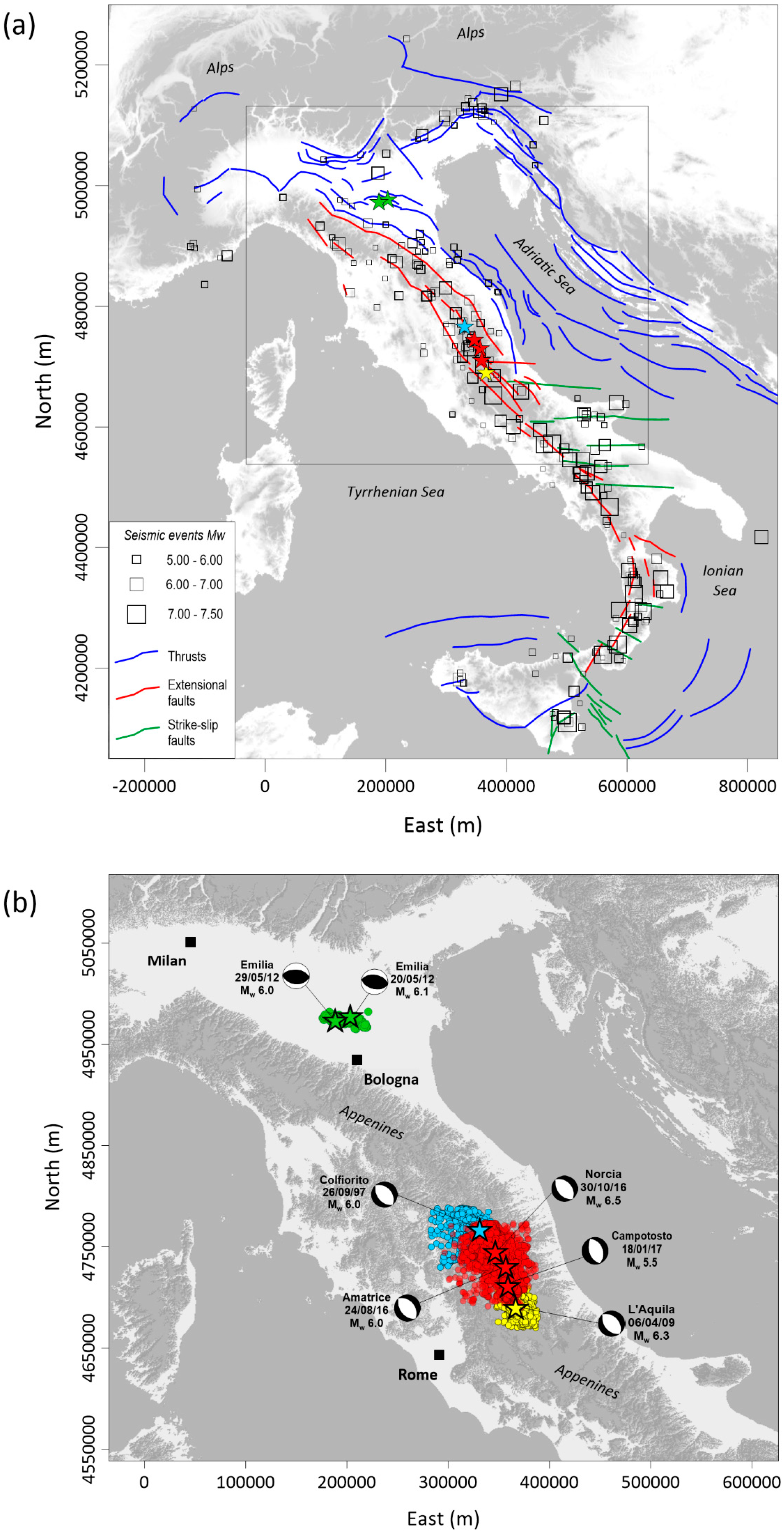
2.2.1. The Colfiorito Seismic Sequence
The ground displacements caused by the M
w 6.0 Colfiorito earthquake (26 September 1997) have been analyzed through DInSAR measurements acquired by the European Remote-Sensing Satellite (ERS) from descending pass.
Figure 2 shows the deformation map, which is relevant to the SAR acquisitions of 7 September and 12 October 1997 [
46]. The map reveals a maximum displacement along the radar line of sight (LOS) of about 25 cm. The hanging wall block is affected by the maximum measured subsidence and, in terms of faulting mechanism, this is consistent with a normal slip mechanism.
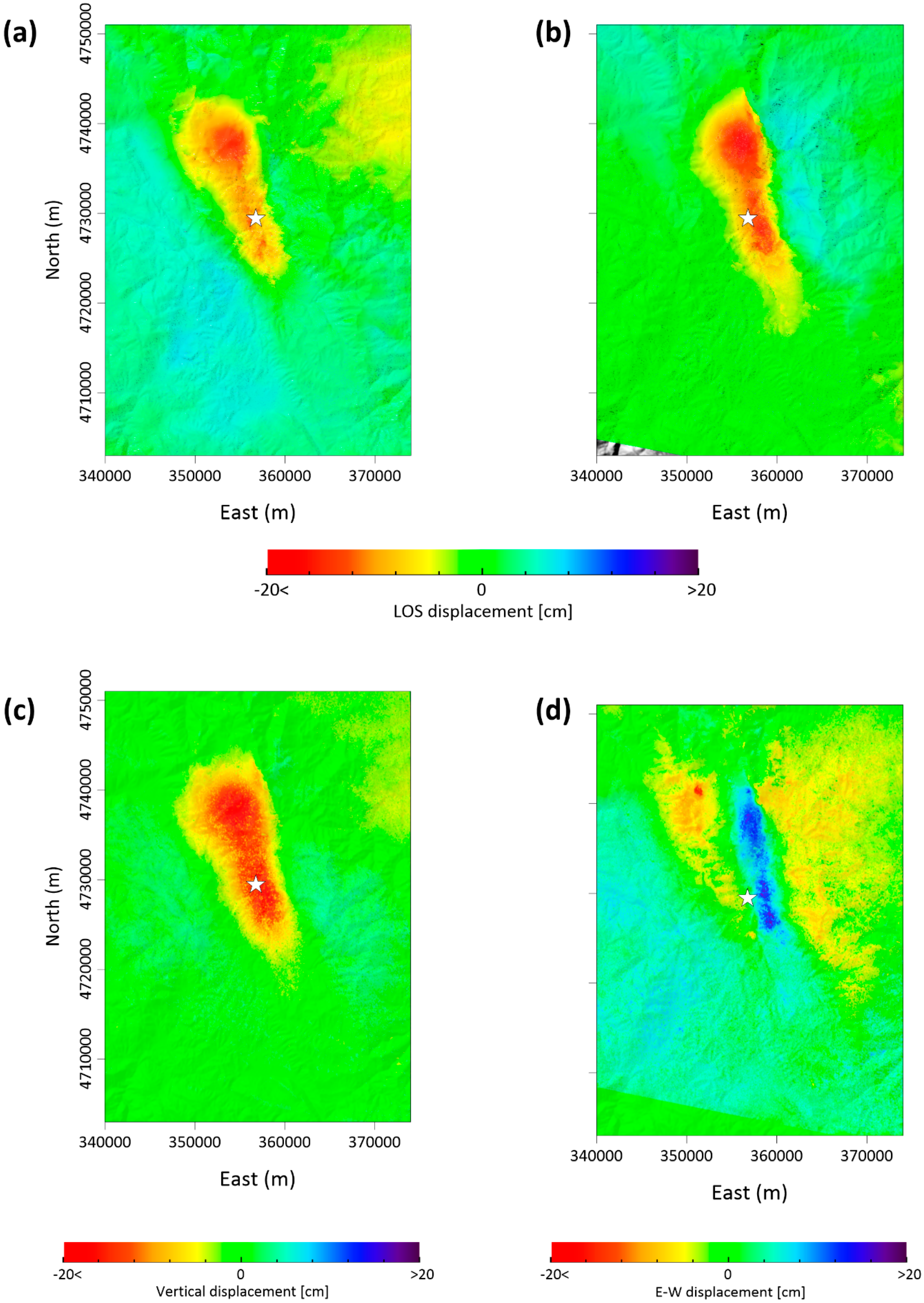
2.2.2. The L’Aquila Seismic Sequence
The ground displacements relevant to the M
w 6.3 L’Aquila earthquake (6 April 2009) have been retrieved through DInSAR measurements acquired by the Environmental Satellite (ENVISAT) from ascending and descending passes (
Figure 3).
Figure 3a,b show the ascending and descending deformation maps, relevant to the acquisitions of 11 March and 15 April 2009 and of 1 February and 12 April 2009, respectively [
47]. These two maps have also been properly combined to retrieve the vertical and the east–west displacement components [
29], which are reported in
Figure 3c,d.
As also discussed in Castaldo et al. [
29], the retrieved deformation pattern (
Figure 3a,b) shows a non-symmetric distribution of the LOS displacements field. The retrieved deformations in the northwestern region reach the value of 17–18 cm and 23–24 cm (corresponding to subsidence processes), for the results relevant to ascending and descending orbits, respectively; moreover, in the northeastern region a maximum displacement of 4–5 cm (corresponding to an uplift of the examined zone) is visible only in the descending map (
Figure 3b). Furthermore, the vertical deformation map reveals a maximum subsidence of about 25 cm that affected the hangingwall block and, in terms of faulting mechanism, this is consistent with a normal slip mechanism.
2.2.3. The Emilia Seismic Sequence
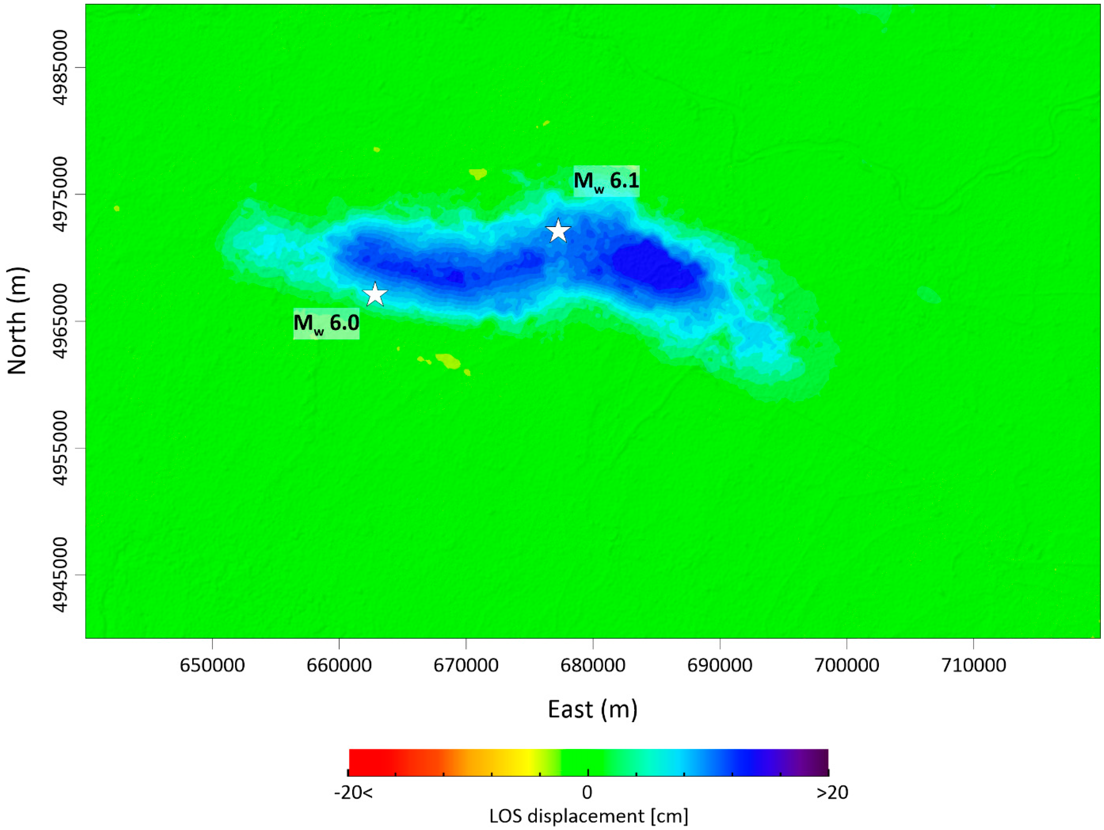
The ground displacements caused by the M
w 6.1 and 6.0 Emilia (20 and 29 May 2012) earthquakes have been studied through DInSAR measurements acquired by the RADARSAT-2 satellite from descending pass (
Figure 4).
Figure 4 shows the deformation map relevant to the acquisitions of 30 April and 17 June 2012; therefore, it has encompassed the two main seismic events [
48]. The deformation map reveals a maximum LOS displacement of about 17 cm (corresponding to un uplift of the considered seismogenic zone). The hanging wall block is affected by the maximum measured uplift and, in terms of faulting mechanism, this is consistent with a reverse slip mechanism.
2.2.4. The Central Italy Seismic Sequence
We analyzed the ground displacements caused by each mainshock of this seismic sequence. In particular, we focused on Sentinel-1 (S1) data acquired over the study area from both ascending and descending orbits. Thanks to their short revisit time and small spatial baseline separation, we selected among the possible interferometric pairs those less affected by undesired phase artifacts (atmospheric phase delays, decorrelation noise, etc.), thus preserving good spatial coverage and interferometric coherence.
In the following, we describe the deformation pattern generated by each earthquake of this seismic sequence.
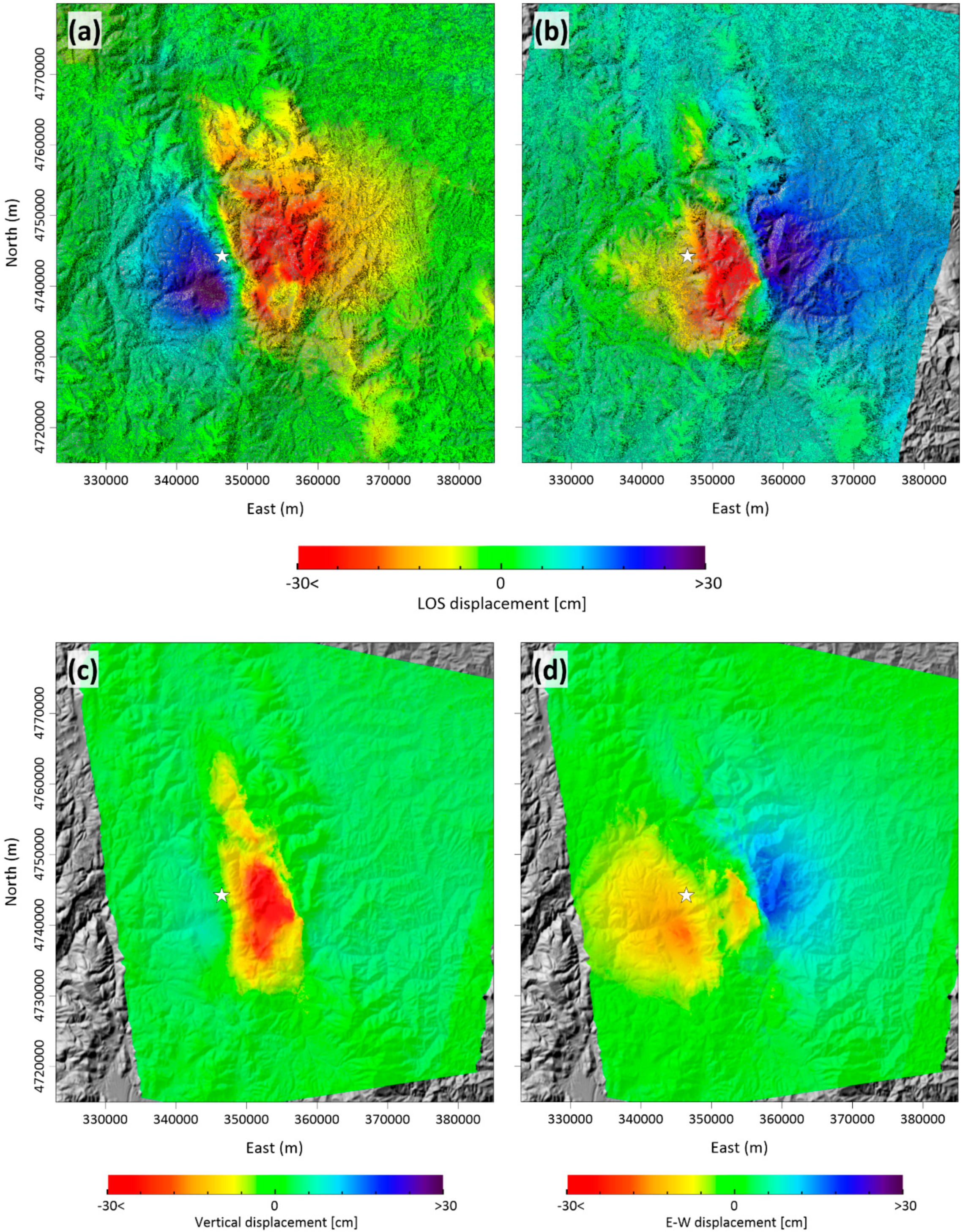
The Amatrice Seismic Sequence
The ground displacements caused by the M
w 6.0 Amatrice earthquake (24 August 2016) have been analyzed through DInSAR measurements acquired by S1 constellation from ascending and descending passes (
Figure 5).
Figure 5a,b show the selected ascending and descending deformation maps, relevant to the acquisitions of 21 and 27 August 2016 and of 15 and 27 August 2016, respectively [
26]. The analysis of these coseismic DInSAR maps revealed a spoon-like shape geometry of the detected surface deformation pattern (
Figure 5) characterized by two NNW–SSE striking main distinctive lobes. The ascending and descending DInSAR maps were also properly combined to retrieve the vertical and the east-west displacement components, which are reported in
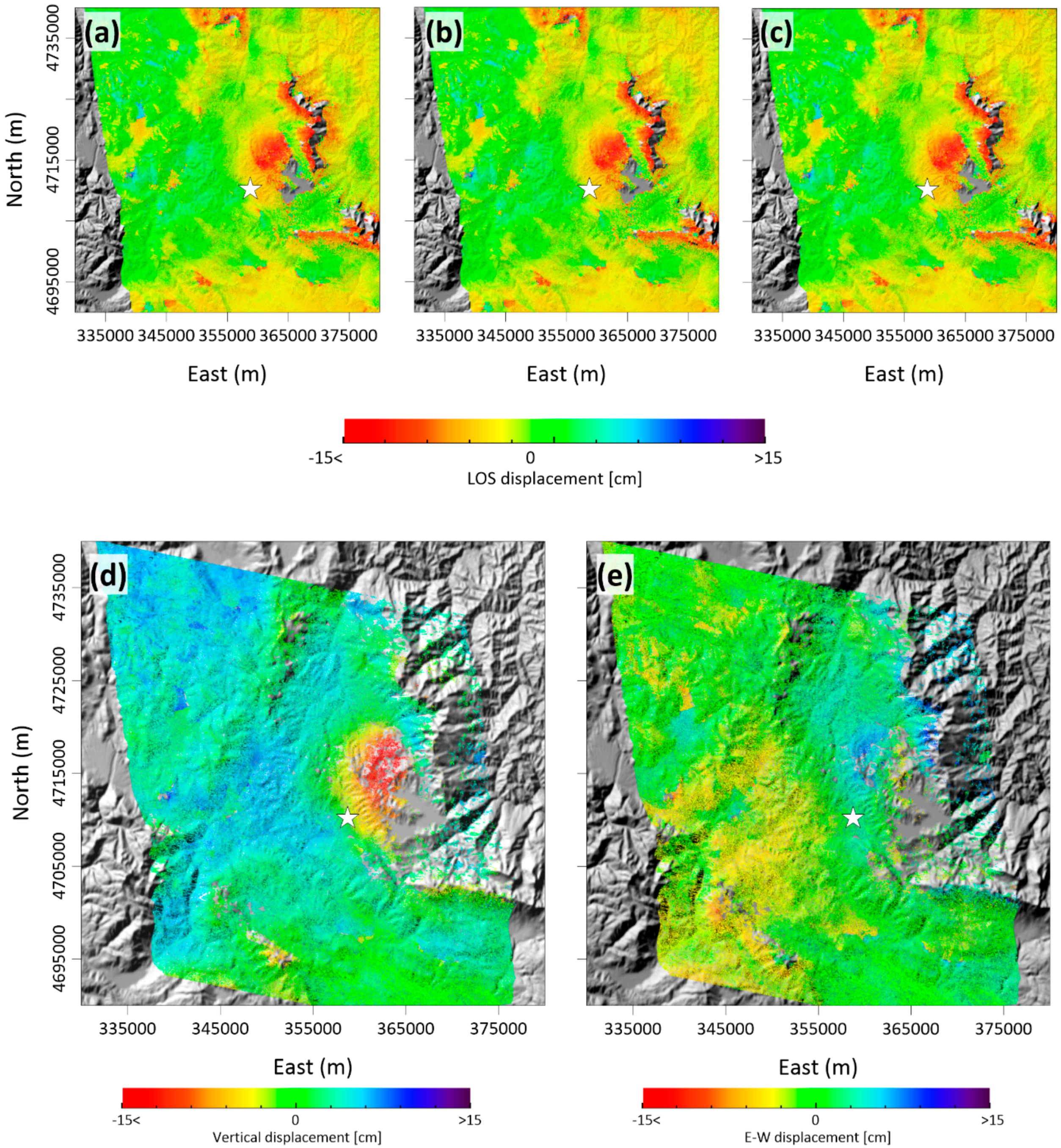
Figure 5c,d. The vertical deformation map reveals a maximum subsidence of about 20 cm that affected the hangingwall block and, in terms of faulting mechanism, this is consistent with a normal slip mechanism.
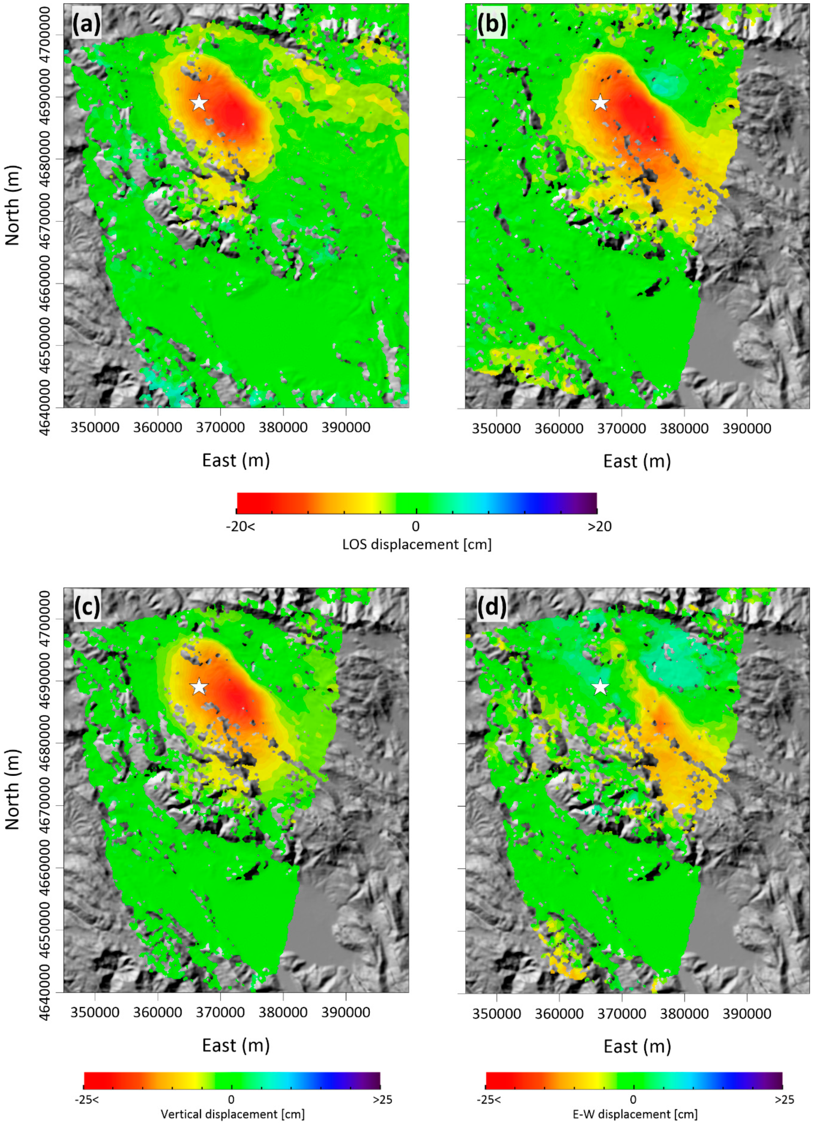
The Norcia Seismic Sequence
The ground displacements caused by the M
w 6.5 Norcia earthquake (30 October 2016) have been examined through DInSAR measurements acquired by S1 constellation from ascending and descending passes (
Figure 6). As in the case of the Amatrice earthquake, we focused on S1 SAR data acquired on 26 October and 1 November 2016 along ascending and descending orbits (
Figure 6a,b) [
28]. The analysis of these coseismic DInSAR measurements revealed two NNW–SSE- striking main lobes. The ascending and descending DInSAR maps were also combined to retrieve the vertical and the east-west displacement components, which are reported in
Figure 6c,d. In particular, the vertical deformation map revealed a maximum subsidence of about 70 cm that affected the hangingwall block, and also a maximum uplift of about 10 cm that affected the adjacent footwall block (
Figure 6c). These are the biggest ground deformations ever measured in Italy by using the DInSAR technique and caused by an earthquake. In terms of faulting mechanism, the measured ground displacements are consistent with a normal slip mechanism.
The Campotosto Seismic Sequence
The ground displacements caused by the M
w 5.5 Campotosto earthquake (18 January 2017) have been studied through DInSAR measurements acquired by the ALOS-2 satellite from ascending and descending passes and S1 constellation from ascending pass (
Figure 7). The ALOS-2 measurements were acquired on 2 November 2016 and 25 January 2017 and on 9 November 2016 and 15 February 2017 along ascending and descending orbits, respectively (
Figure 7a,b), and the S1 measurements were captured on 12 January and 24 January 2017 along the ascending orbit (
Figure 7c). The ascending and descending maps were also combined to retrieve the vertical and the east-west displacement components, which are reported in
Figure 7c,d. In particular, the vertical deformation map revealed a maximum subsidence of about 15 cm that affected the hangingwall block (
Figure 7d). In terms of faulting mechanism, the measured ground displacements are consistent with a normal slip mechanism.
3. Employed Method
We examined faulting and fragmentation processes by using the Fractals Theory [
19,
20,
23]. In this context, the fractal geometries are strictly related to the faulting processes caused by earthquake nucleation. The variation of fractal parameters can thus be indicative of the temporal and spatial evolution of the fragmentation processes along a fault system in time and space. We analyzed the seismological data presented in
Section 2.1 (in particular, the magnitude–frequency distribution of earthquakes) by using a dedicated software, fitting the same data with a power law, and obtaining the fractal dimension and the related coefficient of determination (i.e., R-squared or R
2).
The equation relevant to the above mentioned power law is:
where
Ni is the number of objects with a characteristic linear dimension
ri,
C is a constant of proportionality, and
D is the fractal dimension (in our case,
Ni is the number of earthquakes with a certain magnitude ranges
ri).
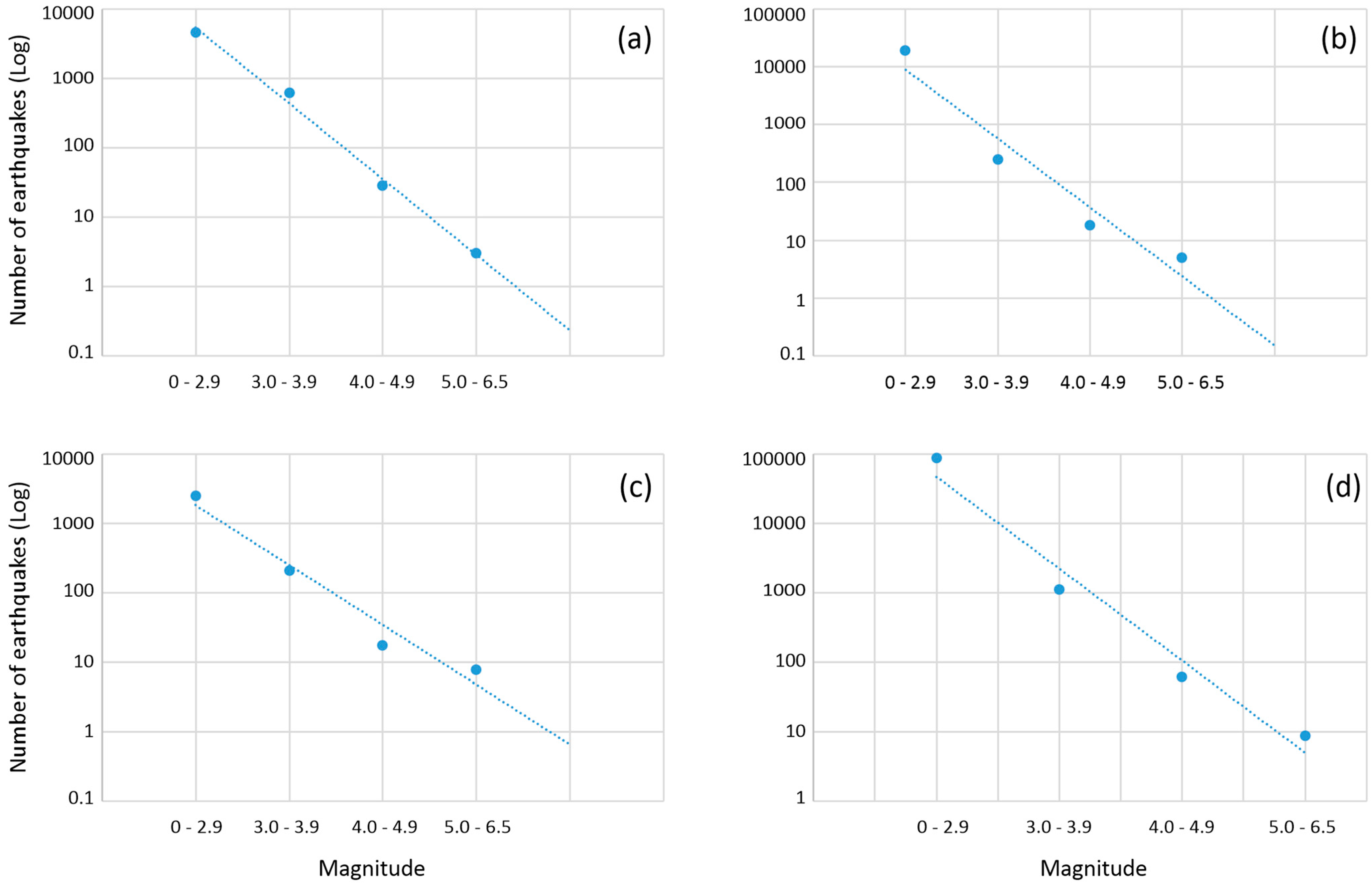
For each seismic sequence, we realized semi-logarithmic graphs, in which we reported the number of earthquakes occurred in certain magnitude ranges (
Figure 8 and
Figure S4). In particular, we plotted the number of earthquakes on the y-axis by using a logarithmic scale and the correspondent magnitude range on the x-axis. According to Equation (1), we searched for the exponential curve that best fits the considered data. Since we worked in a semi-logarithmic space, this exponential curve turns in a straight line (see dotted line in
Figure 8 and
Figure S4). All the unknown parameters of Equation (1), and in particular the fractal dimension, directly derive from the performed best-fit operation.
According to this topological analysis, the fractal dimension value represents the level of irregularity of the selected fractal set [
23] and is indicative of the fragmentation process that occurred during the mainshock and the following aftershocks. If D = 0, it represents the classical Euclidean dimension of a point; if D = 1, the dimension of a line segment; if D = 2, the dimension of a surface and, finally, if D = 3, the Euclidean dimension of a volume [
23,
49]. To check data accuracy, we calculated the coefficient of determination (R-squared) connected with Equation (1) for each seismic sequence. R-squared represents the variability between data instability and model accuracy and can range between 0 and 1. The higher the R-squared values, the higher the model accuracy; therefore, high R-squared values point to a good fit between the model accuracy and the data instability.
4. Results
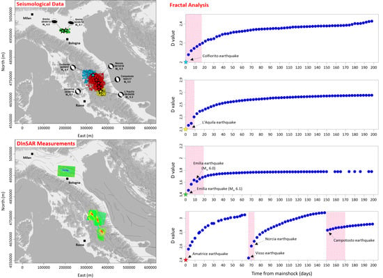
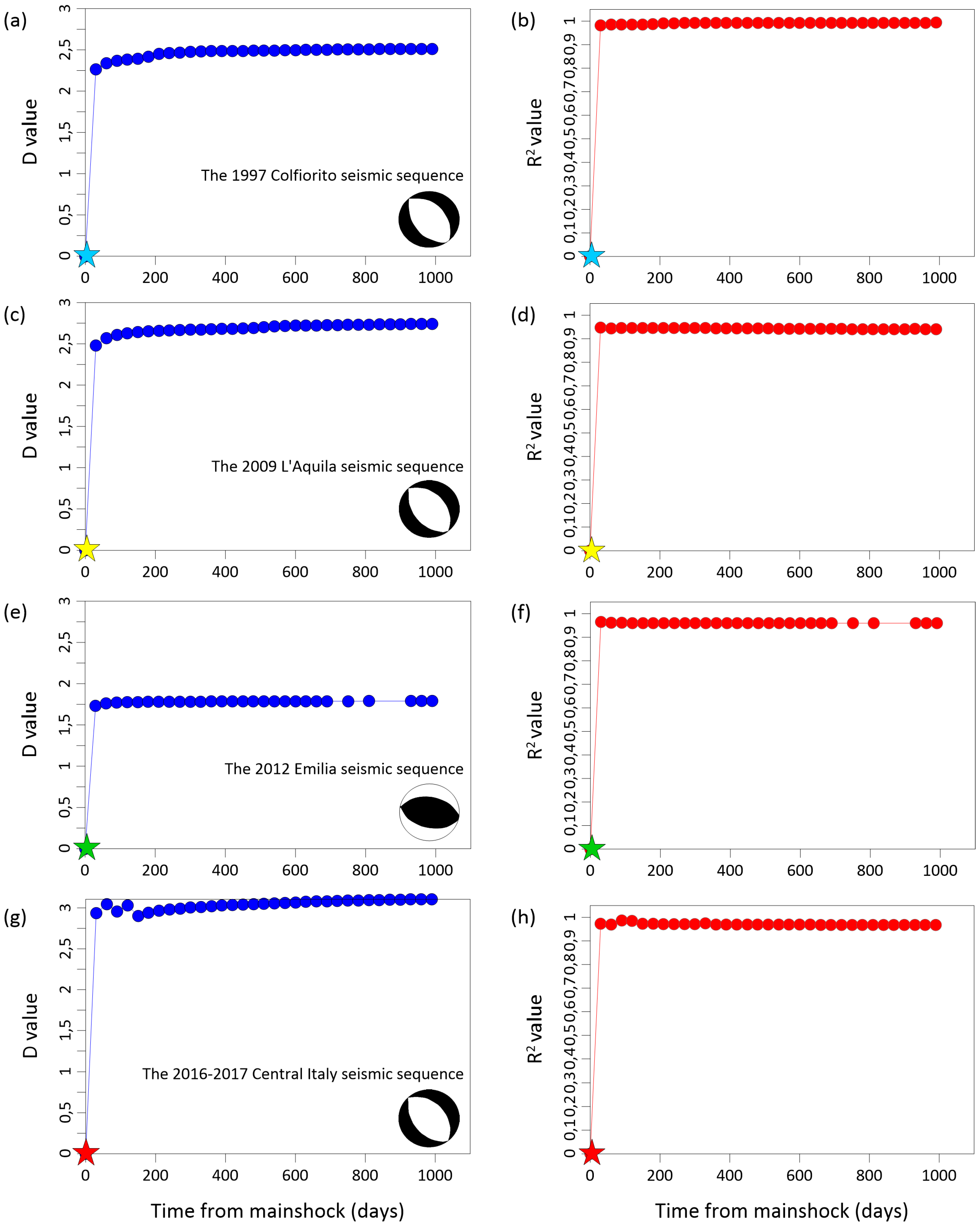
The results retrieved from the application of the Fractals Theory show some significant aspects about seismic sequences and, in particular, about the nature and classification of the faulting processes active during the considered Italian seismic sequences with comparable magnitude. In particular, the analyses of the seismic sequences, performed through the fractal dimension computation within a 1000 days time-lapse, reveal that:
In the case of the 1997 Colfiorito seismic sequence, the fractal dimension assumes an initial value of about 2.3 and reaches a maximum value of about 2.55; as regards the R-squared, its values range between about 0.982 and 0.9935 at the beginning and at the end of the established time interval, respectively.
In the case of the 2009 L’Aquila seismic sequence, the fractal dimension assumes an initial value of about 2.48 and reaches a maximum value of about 2.75; as regards the R-squared, its values range between about 0.9475 and 0.9415 at the beginning and at the end of the established time interval, respectively.
In the case of the 2012 Emilia seismic sequence, the fractal dimension assumes an initial value of about 1.73 and reaches a maximum value of about 1.79; as regards the R-squared, its values range between about 0.965 and 0.96 at the beginning and at the end of the established time interval, respectively.
In the case of the 2016–2017 Central Italy seismic sequence, the fractal dimension assumes an initial value of about 2.9 and reaches a maximum value of about 3.05; as regards the R-squared, its values range between about 0.973 and 0.968 at the beginning and at the end of the established time interval, respectively.
To summarize, we highlight that these values vary between ca. 2–3 and ca. 1–2 for extensional (i.e., the 1997 Colfiorito, the 2009 L’Aquila and the 2016–2017 Central Italy seismic sequences) and compressional seismic sequences (i.e., the 2012 Emilia seismic sequence), respectively (
Figure 9a,c,e,g and
Figure 10). As the fractal dimension is indicative of the geometrical features of a faulting process [
23,
49], it means that over time extensional seismic sequences are thus spatially distributed within a volume, whereas compressional ones are aligned along a preferential rupture surface.
Moreover, we show that the average coefficient of determination R-squared is greater than 0.94 for all the analyzed seismic sequences (
Figure 9b,d,f,h and
Figure S3); these high R-squared values indicate both that the retrieved results are robust and that the exploited seismological catalog presents a good completeness.
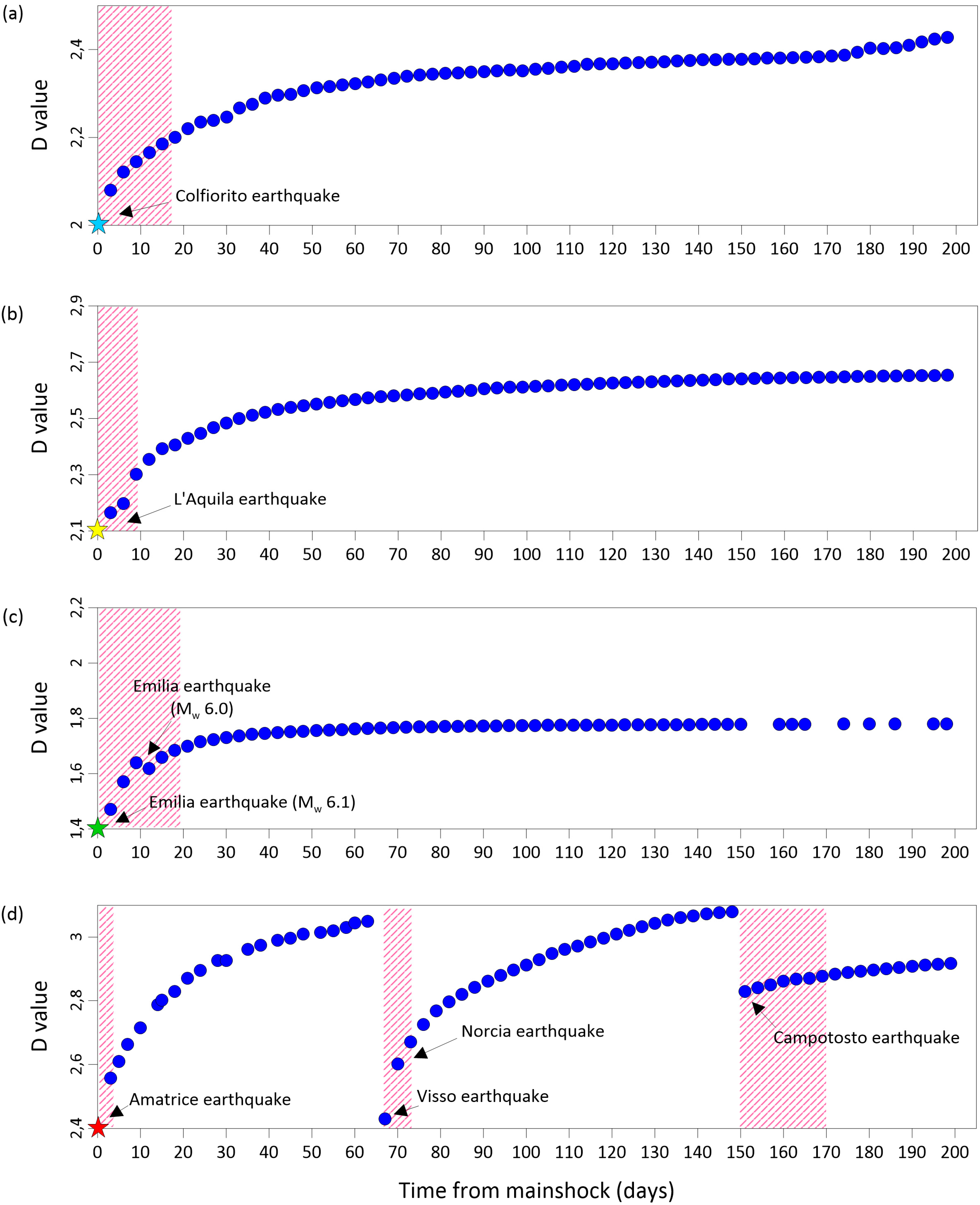
As visible in
Figure 10, our detailed fractal dimension analysis (200 days) reveals that the examined faulting processes can be considered auto-similar during their temporal evolution. This tendency can be observed both in the case of a singular faulting process with one medium-high intensity mainshock (i.e., the 1997 Colfiorito, the 2009 L’Aquila and the 2012 Emilia seismic sequences) and of articulated sequences, characterized by the spatial activation of more fault segments over time (i.e., the 2016–2017 Central Italy seismic sequence). Moreover, from the beginning of the considered observation time interval (i.e., from the mainshock) the fractal dimension presents initial values decisively greater than 2 in the case of the extensional seismic sequences (
Figure 10a,b,d), whereas these values are smaller than 2 in the case of compressional seismic sequences, also after a long period following the mainshock occurrence (
Figure 10c).
5. Discussion
Starting from the results retrieved from the fractal dimension computation (i.e., fractal dimension values vary between ca. 2–3 and ca. 1–2 for extensional and compressional earthquakes, respectively), we show that over time extensional seismic sequences are thus spatially distributed within a volume, whereas compressional ones are aligned along a preferential rupture surface.
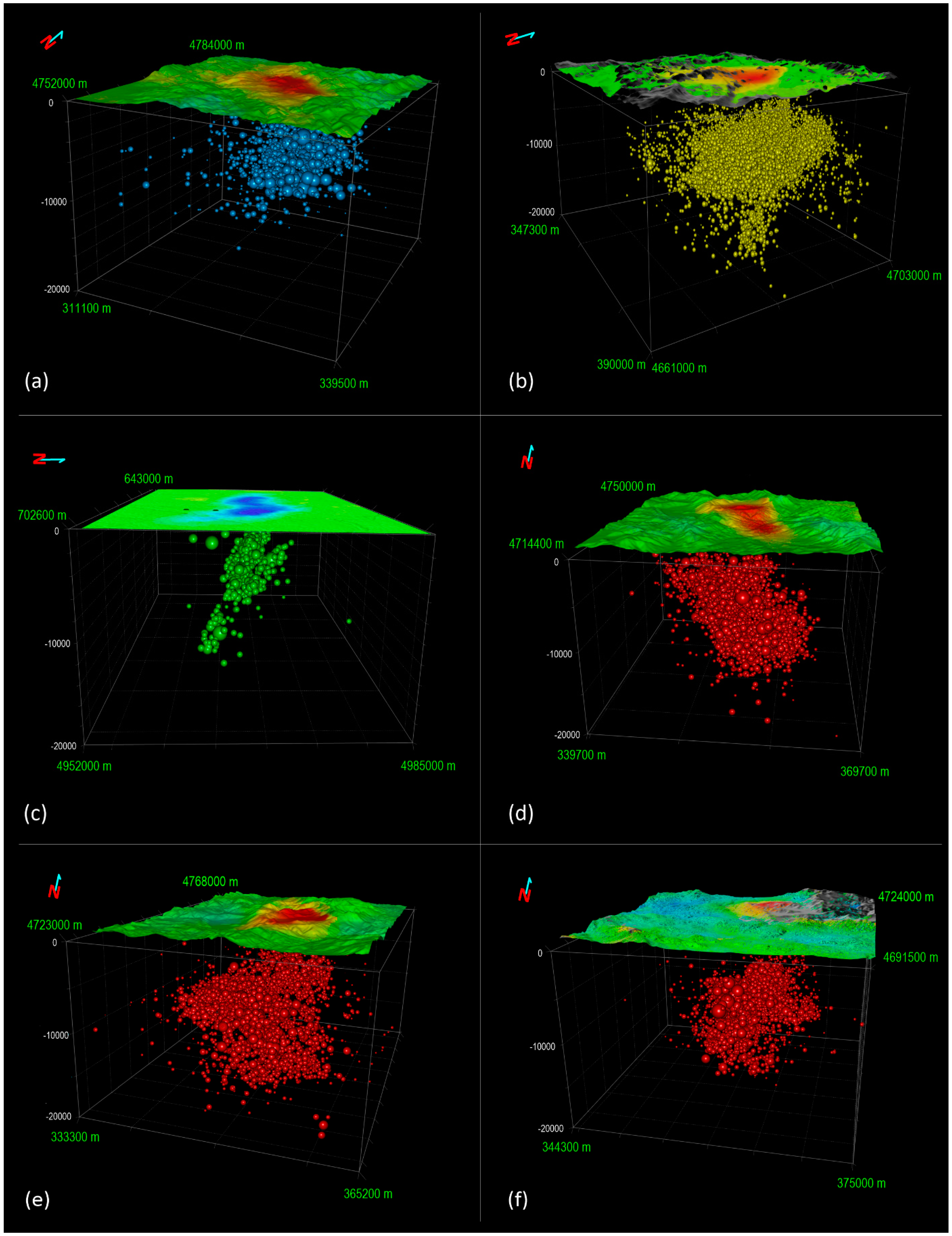
The validity of the retrieved fractal dimension results is confirmed by correlating the 3D hypocentral spatial distribution of the earthquakes occurred in the time interval ranging between the mainshock and the post-seismic SAR acquisition (time-lapse corresponding to the red dashed areas in
Figure 10), and the coseismic DInSAR ground deformation maps, see
Figure 11. Indeed, we observe that in the case of the extensional seismic sequences the hypocenters present a volumetric distribution, which occupies the involved hangingwall rock block (
Figure 11a,b,d,e,f); conversely, in the case of the compressional seismic sequences, the hypocenters distribution reveals a good and preferential alignment along the involved seismogenic fault (
Figure 11c).
We also emphasize that the coseismic deformation patterns present different characteristics for extensional and compressional seismic sequences (see
Figure 2,
Figure 3,
Figure 4,
Figure 5,
Figure 6 and
Figure 7). Specifically, in the first case the ground deformation pattern is typically an image of the crustal block involvement during faulting processes [
29]; accordingly, the deformation pattern retrieved on the Earth’s surface is significantly spatially extended with respect to the main fault location (
Figure 2,
Figure 3,
Figure 5,
Figure 6,
Figure 7 and
Figure 11a,b,d,e,f) [
26,
28,
29,
30]. Conversely, in the second case the observed ground deformation pattern is strictly linked to the fault geometry; therefore, the measured ground deformation pattern is spatially less extended with respect to the main fault location (
Figure 4 and
Figure 11c) [
48]. This evidence may support the different fractal dimension values that, in turn, can be considered as a signature of different evolution of fragmentation mechanism.
The performed joint analyses provide a clear image of the faulting processes consequent to the mainshock nucleation, thus suggesting the possibility to conceive the evolution of the activated faulting process also starting from the first days of the considered seismic sequences.
Finally, we propose that the different features highlighted by our analyses can be related to the different types of energy released during the earthquakes, in turn associated with the tectonic setting [
24]. In particular, we suggest that extensional seismic sequences mainly dissipate gravitational energy, stored during the interseismic period, and the consequent downward hangingwall block movement is favored by gravity. This induces an increase of potential energy and facilitates fracturing processes during the coseismic phase; the potential energy is converted into kinetic energy as indicated by the double-couple mechanism of the earthquakes generated by the shear on the fault planes. In this case, most of the involved forces are distributed within the fault hangingwall block, implying a volumetric distribution of the occurred seismic events. On the contrary, we suggest that the compressional seismic sequences are characterized by dissipation of elastic energy, which is stored both within the rock volume above the thrust fault (i.e., the hangingwall block) and along the thrust fault itself during the interseismic period. The elastic energy dissipation is buffered by the gravitational force and the downward directed gravitational force is opposite to the upward sense of motion of the hangingwall. Therefore, to overcome the inertial system, most of the stored energy is used to activate the main fault, stresses are concentrated at the interface between hangingwall and footwall blocks (i.e., along the thrust) and, therefore, earthquakes nucleate in correspondence of the seismogenic thrust, showing a preferential alignment along the involved structure.
6. Conclusions
In this work, we have performed a detailed analysis of four seismic sequences that occurred in the Italian peninsula during the last 20 years (1997 to 2017) with Mw ≥ 5.5 mainshocks, and we have jointly exploited the available seismological data and DInSAR measurements, in order to investigate the different features of faulting mechanism (i.e., compressional and extensional tectonic settings).
Our main findings can be summarized as follows:
We have employed the fractal analysis to investigate the fragmentation processes caused by earthquake nucleation, which is related in turn to the temporal variation of the fractal dimension values.
The analyses of the fractal dimension values show that over time extensional seismic sequences (i.e., the 1997 Colfiorito, the 2009 L’Aquila and the 2016–2017 Central Italy seismic sequences) are spatially distributed within a volume, whereas compressional ones (i.e., the 2012 Emilia seismic sequence) are aligned along a preferential rupture surface. This is clearly highlighted by the hypocentral spatial distribution of the events, as well as from the surficial spatial extensions of DInSAR coseismic deformation maps.
Our fractal dimension analysis suggests that the studied seismic sequences reveal an auto-similar tendency during their temporal evolution, in the case of both singular faulting processes and articulated ones; moreover, the retrieved fractal dimension values furnish a clear image of the faulting processes consequent to the mainshock occurrence, within compressional and extensional settings.
This joint analysis has allowed us to typify different Italian geodynamic contexts and to provide new insights into the faulting processes caused by the considered seismic sequences.
Supplementary Materials
The following are available online at
https://0-www-mdpi-com.brum.beds.ac.uk/2072-4292/11/18/2112/s1, Figure S1: Magnitude vs. Time. Magnitude distribution versus time in the case of (a) the 1997 Colfiorito, (b) the 2009 L’Aquila earthquake, (c) the 2012 Emilia and (d) the 2016–2017 Central Italy seismic sequences. The days from the mainshock and the magnitude values are shown on the x-axis and are shown on the y-axis, respectively. Figure S2: Interferometric SAR data pairs. Timesheet and coseismic interferometric SAR data pairs exploited for the analysis. The M
w 6.0 Colfiorito, the M
w 6.3 L’Aquila, the M
w 6.1 Emilia mainshocks are represented by the light blue, yellow and green stars, respectively; the Central Italy mainshocks (i.e., the M
w 6.0 Amatrice, the M
w 6.5 Norcia and the M
w 5.5 Campotosto earthquakes) are highlighted by the red stars. Figure S3: R-squared analysis on a 200 days time-lapse. Detailed analysis (200 days) of the R-squared temporal evolution in the case of (a) the 1997 Colfiorito, (b) the 2009 L’Aquila, (c) the 2012 Emilia and (d) the 2016–2017 Central Italy seismic sequences. Figure S4: Application of the Fractal Theory. Example of the application of the Fractal Theory in the case of the 1997 Colfiorito seismic sequence. The number of earthquakes (logarithmic scale) occurred in certain magnitude ranges is reported in the graphs and the dotted lines represent the simple linear regression. Table S1: Retrieved DInSAR displacement values of the considered seismic sequences.
Author Contributions
Conceptualization: E.V., P.T.; Data curation: E.V., V.D.N., M.M.; Methodology: E.V., P.T.; Software: E.V., V.D.N., M.M.; Supervision: M.M., P.T.; Validation: E.V., P.T.; Visualization: E.V., V.D.N.; Writing—draft: E.V., V.D.N., M.M.; Writing—review and editing: E.V., V.D.N., M.M., P.T.
Funding
This research received no external funding.
Acknowledgments
This work has been supported by the DPC-IREA Agreement, the CNR project “Development and application of geo-physical method based on the use of remote-sensing data (DTA.AD004.065)-subproject “Modeling of Geophysical processes” (DTA.AD004.065.001) and the I-AMICA project (Infrastructure of High Technology for Environmental and Climate Monitoring-PONa3_00363). The ERS and ENVISAT, and RADARSAT-2 data have been provided by the European Space Agency and the Canadian Space Agency, respectively. Sentinel-1 data have been furnished through the Copernicus Program of the European Union. The ALOS-2 data have been provided by JAXA through the Announcement of Opportunity (AO) RA-6 PI No.3184. The DEM of the investigated zones were acquired through the SRTM archive.
Conflicts of Interest
The authors declare no conflict of interest.
References
- Basili, R.; Valensise, G.; Vannoli, P.; Burrato, P.; Fracassi, U.; Mariano, S.; Tiberti, M.M.; Boschi, E. The Database of Individual Seismogenic Sources (DISS), version 3: Summarizing 20 years of research on Italy’s earthquake geology. Tectonophysics 2008, 453, 20–43. [Google Scholar] [CrossRef]
- Burrato, P.; Poli, M.E.; Vannoli, P.; Zanferrari, A.; Basili, R.; Galadini, F. Sources of Mw 5+ earthquakes in northeastern Italy and western Slovenia: An updated view based on geological and seismological evidence. Tectonophysics 2008, 453, 157–176. [Google Scholar] [CrossRef]
- Liu, X.J.; Zhan, F.B.; Hong, S.; Niu, B.; Liu, Y. A bibliometric study of earthquake research: 1900–2010. Scientometrics 2012, 92, 747–765. [Google Scholar] [CrossRef]
- Rovida, A.; Locati, M.; Camassi, R.; Lolli, B.; Gasperini, P. (Eds.) CPTI15, the 2015 Version of the Parametric Catalogue of Italian Earthquakes; Istituto Nazionale di Geofisica e Vulcanologia: Rome, Italy, 2016. [Google Scholar] [CrossRef]
- Carminati, E.; Doglioni, C. Alps vs. Apennines: The paradigm of a tectonically asymmetric Earth. Earth-Sci. Rev. 2012, 112, 67–96. [Google Scholar] [CrossRef]
- Doglioni, C. A proposal for the kinematic modelling of W-dipping subductions-possible applications to the Tyrrhenian-Apennines system. Terra Nova 1991, 3, 423–434. [Google Scholar] [CrossRef]
- Vannoli, P.; Burrato, P.; Valensise, G. The seismotectonics of the Po Plain (northern Italy): Tectonic diversity in a blind faulting domain. Pure Appl. Geophys. 2015, 172, 1105–1142. [Google Scholar] [CrossRef]
- Carminati, E.; Lustrino, M.; Doglioni, C. Geodynamic evolution of the central and western Mediterranean: Tectonics vs. igneous petrology constraints. Tectonophysics 2012, 579, 173–192. [Google Scholar] [CrossRef]
- Cavinato, G.P.; Celles, P.D. Extensional basins in the tectonically bimodal central Apennines fold-thrust belt, Italy: Response to corner flow above a subducting slab in retrograde motion. Geology 1999, 27, 955–958. [Google Scholar] [CrossRef]
- Chiaraluce, L. Unravelling the complexity of Apenninic extensional fault systems: A review of the 2009 L’Aquila earthquake (Central Apennines, Italy). J. Struct. Geol. 2012, 42, 2–18. [Google Scholar] [CrossRef]
- Devoti, R.; Pietrantonio, G.; Pisani, A.R.; Riguzzi, F.; Serpelloni, E. Present day kinematics of Italy. J. Virtual Expl. 2010, 36. [Google Scholar] [CrossRef]
- Montone, P.; Mariucci, M.T.; Pierdominici, S. The Italian present-day stress map. Geophys. J. Int. 2012, 189, 705–716. [Google Scholar] [CrossRef] [Green Version]
- Montone, P.; Mariucci, M.T. The new release of the Italian contemporary stress map. Geophys. J. Int. 2016, 205, 1525–1531. [Google Scholar] [CrossRef]
- Guidarelli, M.; Panza, M.G. INPAR, CMT and RCMT seismic moment solutions compared for the strongest damaging events (M ≥ 4.8) occurred in the Italian region in the last decade. Rendic. Acc. Naz. Sci. Detta Dei XL 2006, 124, 81–98. [Google Scholar]
- Petricca, P.; Barba, S.; Carminati, E.; Doglioni, C.; Riguzzi, F. Graviquakes in Italy. Tectonophysics 2015, 656, 202–214. [Google Scholar] [CrossRef]
- Devoti, R.; Riguzzi, F. The velocity field of the Italian area. Rend. Lincei Sci. Fis. Nat. 2018, 29, 51–58. [Google Scholar] [CrossRef]
- King, G.C.P. The accommodation of large strains in the upper lithosphere of the earth and other solids by self-similar fault systems: The geometrical origin of b-value. Pure Appl. Geophys. 1983, 121. [Google Scholar] [CrossRef]
- King, G.C.P. Speculations on the geometry of the initiation and terminationprocesses of earthquake rupture and its relation to morphology and geological structure. Pure Appl. Geophys. 1986, 124, 567–585. [Google Scholar] [CrossRef]
- Turcotte, D.L. Fractals and fragmentation. J. Geophys. Res. 1986, 91, 1921–1926. [Google Scholar] [CrossRef]
- Turcotte, D.L. A fractal model for crustal deformation. Tectonophysics 1986, 132, 261–269. [Google Scholar] [CrossRef]
- King, G.C.P.; Stein, R.S.; Rundle, J.B. The growth of geological structures by repeated earthquakes 1. Conceptual framework. J. Geophys. Res. 1988, 93, 13307–13318. [Google Scholar] [CrossRef]
- Hirata, T. Fractal dimension of fault systems in Japan: Fractal structure in rock fracture geometry at various scales. Pure Appl. Geophys. 1989, 131, 157–170. [Google Scholar] [CrossRef]
- Mandelbrot, B.B. Multifractal measures, especially for the geophysicist. Pure Appl. Geophys. 1989, 131, 5–42. [Google Scholar] [CrossRef]
- Valerio, E.; Tizzani, P.; Carminati, E.; Doglioni, C. Longer aftershocks duration in extensional tectonic settings. Sci. Rep. 2017, 7. [Google Scholar] [CrossRef] [PubMed]
- Salvi, S.; Stramondo, S.; Cocco, M.; Tesauro, M.; Hunstad, I.; Anzidei, M.; Briole, P.; Baldi, P.; Sansosti, E.; Fornaro, G.; et al. Modeling coseismic displacements resulting from SAR interferometry and GPS measurements during the 1997 Umbria-Marche seismic sequence. J. Seism. 2000, 4, 479–499. [Google Scholar] [CrossRef]
- Lavecchia, G.; Castaldo, R.; De Nardis, R.; De Novellis, V.; Ferrarini, F.; Pepe, S.; Brozzetti, F.; Solaro, G.; Cirillo, D.; Bonano, M.; et al. Ground deformation and source geometry of the 24 August 2016 Amatrice earthquake (Central Italy) investigated through analytical and numerical modeling of DInSAR measurements and structural-geological data. Geophys. Res. Lett. 2016, 43, 12–389. [Google Scholar] [CrossRef]
- Cheloni, D.; Giuliani, R.; D’Agostino, N.; Mattone, M.; Bonano, M.; Fornaro, G.; Lanari, R.; Reale, D.; Atzori, S. New insights into fault activation and stress transfer between en echelon thrusts: The 2012 Emilia, Northern Italy, earthquake sequence. J. Geophys. Res. Solid Earth 2016, 121, 4742–4766. [Google Scholar] [CrossRef] [Green Version]
- Cheloni, D.; De Novellis, V.; Albano, M.; Antonioli, A.; Anzidei, M.; Atzori, S.; Avallone, A.; Bignami, C.; Bonano, M.; Calcaterra, S.; et al. Geodetic model of the 2016 Central Italy earthquake sequence inferred from InSAR and GPS data. Geophys. Res. Lett. 2017, 44, 6778–6787. [Google Scholar] [CrossRef]
- Castaldo, R.; De Nardis, R.; Ferrarini, F.; Lanari, R.; Lavecchia, G.; Pepe, S.; Solaro, G.; Tizzani, P.; De Novellis, V. Coseismic Stress and Strain Field Changes Investigation through 3-D Finite Element Modeling of DInSAR and GPS Measurements and Geological/Seismological Data: The L’Aquila (Italy) 2009 Earthquake Case Study. J. Geophys. Res. Solid Earth 2018, 123, 4193–4222. [Google Scholar] [CrossRef]
- Valerio, E.; Tizzani, P.; Carminati, E.; Doglioni, C.; Pepe, S.; Petricca, P.; De Luca, C.; Bignami, C.; Solaro, G.; Castaldo, R.; et al. Ground Deformation and Source Geometry of the 30 October 2016 Mw 6.5 Norcia Earthquake (Central Italy) Investigated through Seismological Data, DInSAR Measurements, and Numerical Modelling. Remote Sens. 2018, 10, 1901. [Google Scholar] [CrossRef]
- DISS Working Group. Database of Individual Seismogenic Sources (DISS), Version 3.2.1: A Compilation of Potential Sources for Earthquakes Larger Than M 5.5 in Italy and Surrounding Areas. Istituto Nazionale di Geofisica e Vulcanologia. 2018. Available online: http://diss.rm.ingv.it/diss/ (accessed on 10 September 2019). [CrossRef]
- ISIDe Working Group (2016) Version 1.0. Available online: http://terremoti.ingv.it/ (accessed on 10 September 2019). [CrossRef]
- Amato, A.; Azzara, R.; Chiarabba, C.; Cocco, M.; Di Bona, M.; Mele, F.; Basili, A.; Boschi, E.; Deschamps, A.; Gaffet, S.; et al. The 1997 Umbria-Marche, Italy, earthquake sequence: A first look at the main shocks and aftershocks. Geophys. Res. Lett. 1998, 25, 2861–2864. [Google Scholar] [CrossRef]
- Ripepe, M.; Piccinini, D.; Chiaraluce, L. Foreshock sequence of September 26th, 1997 Umbria-Marche earthquakes. J. Seismol. 2000, 4, 387–399. [Google Scholar] [CrossRef]
- Ferrarini, F.; Lavecchia, G.; de Nardis, R.; Brozzetti, F. Fault geometry and active stress from earthquakes and field geology data analysis: The Colfiorito 1997 and L’Aquila 2009 Cases (Central Italy). Pure Appl. Geophys. 2015, 172, 1079–1103. [Google Scholar] [CrossRef]
- Chiaraluce, L.; Chiarabba, C.; De Gori, P.; Di Stefano, R.; Improta, L.; Piccinini, D.; Schlagenhauf, A.; Traversa, P.; Valoroso, L.; Voisin, C. The 2009 L’Aquila (Central Italy) Seismic Sequence. Boll. Geofis. Teor. Appl. 2010. [Google Scholar] [CrossRef]
- Valoroso, L.; Chiaraluce, L.; Piccinini, D.; Di Stefano, R.; Schaff, D.; Waldhauser, F. Radiography of a normal fault system by 64,000 high-precision earthquake locations: The 2009 L’Aquila (central Italy) case study. J. Geophys. Res. Solid Earth 2013, 118, 1156–1176. [Google Scholar] [CrossRef]
- Scrocca, D.; Carminati, E.; Doglioni, C.; Marcantoni, D. Slab retreat and active shortening along the central-northern Apennines. In Thrust Belts and Foreland Basins; Springer: Berlin/Heidelberg, Germany, 2007. [Google Scholar] [CrossRef]
- Lavecchia, G.; De Nardis, R.; Costa, G.; Tiberi, L.; Ferrarini, F.; Cirillo, D.; Brozzetti, F.; Suhadolc, P. Was the Mirandola thrust really involved in the Emilia 2012 seismic sequence (northern Italy)? Implications on the likelihood of triggered seismicity effects. Boll. Geofis. Teor. Appl. 2015, 56, 461–488. [Google Scholar]
- Chiaraluce, L.; Di Stefano, R.; Tinti, E.; Scognamiglio, L.; Michele, M.; Casarotti, E.; Cattaneo, M.; De Gori, P.; Chiarabba, C.; Monachesi, G.; et al. The 2016 central Italy seismic sequence: A first look at the mainshocks, aftershocks, and source models. Seism. Res. Lett. 2017, 88, 757–771. [Google Scholar] [CrossRef]
- Cheloni, D.; D’Agostino, N.; Scognamiglio, L.; Tinti, E.; Bignami, C.; Avallone, A.; Giuliani, R.; Calcaterra, S.; Gambino, P.; Mattone, M. Heterogeneous Behavior of the Campotosto Normal Fault (Central Italy) Imaged by InSAR GPS and Strong-Motion Data: Insights from the 18 January 2017 Events. Remote Sens. 2019, 11, 1482. [Google Scholar] [CrossRef]
- Massonnet, D.; Rossi, M.; Carmona, C.; Adragna, F.; Peltzer, G.; Feigl, K.; Rabaute, T. The displacement field of the Landers earthquake mapped by radar interferometry. Nature 1993, 364, 138. [Google Scholar] [CrossRef]
- Bamler, R. The SRTM Mission: A World-Wide 30 m Resolution DEM from SAR Interferometry in 11 Days; Fritsch, D., Spiller, R., Eds.; Wichmann Verlang: Heidelberg, Germany, 1999. [Google Scholar]
- Costantini, M. A novel phase unwrapping method based on network programming. IEEE Trans. Geosci. Remote Sens. 1998, 36, 813–821. [Google Scholar] [CrossRef]
- Manzo, M.; Ricciardi, G.; Casu, F.; Ventura, G.; Zeni, G.; Borgström, S.; Berardino, P.; Del Gaudio, C.; Lanari, R. Surface deformation analysis in the Ischia Island (Italy) based on spaceborne radar interferometry. J. Volcanol. Geotherm. Res. 2006, 151, 399–416. [Google Scholar] [CrossRef]
- Stramondo, S.; Tesauro, M.; Briole, P.; Sansosti, E.; Baldi, P.; Fornaro, G.; Avallone, A.; Buongiorno, M.F.; Franceschetti, G.; Boschi, E.; et al. The September 26, 1997 Colfiorito, Italy, earthquakes: Modeled coseismic surface displacement from SAR interferometry and GPS. Geophys. Res. Lett. 1999, 26, 883–886. [Google Scholar] [CrossRef]
- Lanari, R.; Berardino, P.; Bonano, M.; Casu, F.; Manconi, A.; Manunta, M.; Manzo, M.; Pepe, A.; Sansosti, E.; Solaro, G.; et al. Surface displacements associated with the L’Aquila 2009 Mw 6.3 earthquake (central Italy): New evidence from SBAS-DInSAR time series analysis. Geophys. Res. Lett. 2010, 37. [Google Scholar] [CrossRef]
- Tizzani, P.; Castaldo, R.; Solaro, G.; Pepe, A.; Bonano, M.; Casu, F.; Manunta, M.; Manzo, M.; Samsonov, S.; Lanari, R.; et al. New insights into the 2012 Emilia (Italy) seismic sequence through advanced numerical modeling of ground deformation InSAR measurements. Geophys. Res. Lett. 2013, 40, 1971–1977. [Google Scholar] [CrossRef]
- Turcotte, D.L. Fractals and Chaos in Geology and Geophysics; Cambridge University Press: Cambridge, UK, 1997. [Google Scholar]
Figure 1.
Geodynamic context. (
a) Tectonic Map of Italy (WGS84, UTM 33) in which the main tectonic structures (derived from [
31]) are reported and highlighted by different colors as a function of the geodynamic context: extensional faults, thrusts and strike-slip faults are represented by blue, red and green lines, respectively. The historical seismicity is also shown as a function of magnitude (the higher the magnitude, the bigger the squares) [
4]; the mainshocks of the analysed seismic sequences are represented by stars with different colors: the light blue star for the 1997 Colfiorito, the yellow one for the 2009 L’Aquila, the green ones for the 2012 Emilia and the red ones for the 2016–2017 Central Italy mainshocks. The black rectangle indicates the area considered in the following panel. (
b) Seismicity distribution of the 1997 Colfiorito (light blue dots), the 2009 L’Aquila (yellow dots), the 2012 Emilia (green dots) and the 2016–2017 Central Italy (red dots) sequences, superimposed on the 1 arcsec Shuttle Radar Topography Mission (SRTM) digital elevation model (DEM) of the zone. The mainshocks of the analysed seismic sequences are represented by stars and the associated focal mechanisms are also reported in the map.
![Remotesensing 11 02112 g001]()
Figure 2.
DInSAR measurements of the 1997 Colfiorito seismic sequence. DInSAR line-of-sight (LOS) displacement map computed by using ERS images acquired from descending orbits on 7 September–12 October 1997. The white star represents the Mw 6.0 Colfiorito mainshock.
Figure 2.
DInSAR measurements of the 1997 Colfiorito seismic sequence. DInSAR line-of-sight (LOS) displacement map computed by using ERS images acquired from descending orbits on 7 September–12 October 1997. The white star represents the Mw 6.0 Colfiorito mainshock.
Figure 3.
DInSAR measurements of the 2009 L’Aquila seismic sequence. (a,b) DInSAR LOS displacement maps computed by using ENVISAT images acquired from: (a) ascending orbits on 11 March–15 April 2009 and (b) descending orbits on 1 February–12 April 2009. (c,d) Vertical and E-W displacement maps computed by exploiting the ascending and descending ENVISAT measurements shown in panels (a,b). The white star represents the Mw 6.3 L’Aquila mainshock.
Figure 4.
DInSAR measurements of the 2012 Emilia seismic sequence. DInSAR LOS displacement map computed by using RADARSAT-2 images acquired from descending orbits on 30 April–17 June 2012. The white stars represent the Mw 6.1 and Mw 6.0 Emilia mainshocks.
Figure 4.
DInSAR measurements of the 2012 Emilia seismic sequence. DInSAR LOS displacement map computed by using RADARSAT-2 images acquired from descending orbits on 30 April–17 June 2012. The white stars represent the Mw 6.1 and Mw 6.0 Emilia mainshocks.
Figure 5.
DInSAR measurements of the 2016 Amatrice seismic sequence. (a,b) DInSAR LOS displacement maps computed by using S1 images acquired from: (a) ascending orbits on 15 August–27 August 2016 and (b) descending orbits on 21 August–27 August 2016. (c,d) Vertical and E–W displacement maps computed by exploiting the ascending and descending S1 measurements shown in panels (a,b). The white star represents the Mw 6.0 Amatrice mainshock.
Figure 6.
DInSAR measurements of the 2016 Norcia seismic sequence. (a,b) DInSAR LOS displacement maps computed by using S1 images acquired from: (a) ascending orbits and (b) descending orbits both on 26 October–1 November 2016. (c,d) Vertical and E–W displacement maps computed by exploiting the ascending and descending S1 measurements shown in panels (a,b). The white star represents the Mw 6.5 Norcia mainshock.
Figure 7.
DInSAR measurements of the 2017 Campotosto seismic sequence. (a,b) DInSAR LOS displacement maps computed by using ALOS-2 images acquired from: (a) ascending orbits on 2 November 2016–25 January 2017 and (b) descending orbits on 9 November 2016–15 February 2017; (c) DInSAR LOS displacement map computed by using S1 images acquired from ascending orbits on 12 January–24 January 2017. (d,e) Vertical and E-W displacement maps computed by exploiting the ascending and descending ALOS-2 and the ascending S1 measurements shown in panels (a–c). The white star represents the Mw 5.5 Campotosto mainshock.
Figure 8.
Application of fractals theory. Examples of the application of fractals theory in the case of (a) the 1997 Colfiorito, (b) the 2009 L’Aquila, (c) the 2012 Emilia and (d) the 2016–2017 Central Italy seismic sequences. The number of earthquakes (logarithmic scale) occurred in certain magnitude ranges is reported in the graphs and the dotted lines represent the simple linear regression.
Figure 9.
Fractal analysis on a 1000-day time lapse. Fractal dimension temporal evolution and the associated R2 values by considering a 1000-day time-lapse in the case of the (a,b) the 1997 Colfiorito, (c,d) the 2009 L’Aquila, (e,f) the 2012 Emilia and (g,h) the 2016–2017 Central Italy seismic sequences. The Colfiorito, the L’Aquila, the Emilia and the 2016–2017 Central Italy mainshocks are reported with light blue, yellow, green and red stars, respectively.
Figure 10.
Fractal analysis on a 200 days time-lapse. Detailed analysis (200 days) of the fractal dimension temporal evolution shown in
Figure 9 in the case of the (
a) the 1997 Colfiorito, (
b) the 2009 L’Aquila, (
c) the 2012 Emilia and (
d) the 2016–2017 Central Italy seismic sequences. The red dashed areas represent the time interval between the mainshock and the second SAR acquisition (i.e., the second SAR acquisition of the considered DInSAR pair). The Colfiorito, the L’Aquila, the Emilia and the 2016–2017 Central Italy mainshocks are reported with light blue, yellow, green and red stars, respectively.
Figure 11.
3D comparison between DInSAR measurements and earthquakes distribution. 3D view of coseismic displacement maps shown in
Figure 2,
Figure 3c,
Figure 4,
Figure 5c,
Figure 6c and
Figure 7d, and seismicity (the higher the magnitude, the bigger the spheres) recorded during the time interval defined in the red dashed areas in
Figure 10 in the case of (
a) the 1997 Colfiorito (light blue), (
b) the 2009 L’Aquila (yellow), (
c) the 2012 Emilia (green), (
d) the 2016 Amatrice (red), (
e) the 2016 Norcia (red) and (
f) the 2017 Campotosto (red) seismic sequences.
Table 1.
Coseismic interferometric pairs exploited for the Differential Synthetic Aperture Radar Interferometry (DInSAR) analysis of the considered seismic sequences.
Table 1.
Coseismic interferometric pairs exploited for the Differential Synthetic Aperture Radar Interferometry (DInSAR) analysis of the considered seismic sequences.
| Earthquake | Sensor | InSAR Pair | Orbit | Wavelength (cm) | Perpendicular Baseline (m) | Track | Look Angle (deg) |
|---|
| Colfiorito earthquake | ERS | 07091997–12101997 | DESC | 5.56 | 121 | 79 | 23 |
| L’Aquila earthquake | ENVISAT | 11032009–15042009 | ASC | 5.63 | 229 | 129 | 23 |
| ENVISAT | 01022009–12042009 | DESC | 5.63 | −149 | 79 | 23 |
| Emilia earthquake | RADARSAT-2 | 30042012–17062012 | DESC | 5.54 | −477 | | 30 |
| Amatrice earthquake | Sentinel-1 | 15082016–27082016 | ASC | 5.56 | 32 | 117 | 39 |
| Sentinel-1 | 21082016–27082016 | DESC | 5.56 | 79 | 22 | 39 |
| Norcia earthquake | Sentinel-1 | 26102016–01112016 | ASC | 5.56 | 60 | 117 | 36.6 |
| Sentinel-1 | 26102016–01112016 | DESC | 5.56 | 80 | 22 | 39 |
| Campotosto earthquake | Sentinel-1 | 12012017–24012017 | ASC | 5.56 | 16 | 117 | 39 |
| ALOS-2 | 02112016–25012017 | ASC | 24.2 | −59 | 197 | 36.6 |
| ALOS-2 | 09112016–15022017 | DESC | 24.2 | −387 | 92 | 32.8 |
© 2019 by the authors. Licensee MDPI, Basel, Switzerland. This article is an open access article distributed under the terms and conditions of the Creative Commons Attribution (CC BY) license (http://creativecommons.org/licenses/by/4.0/).


