Article

Iterative Pointing Angle Calibration Method for the Spaceborne Photon-Counting Laser Altimeter Based on Small-Range Terrain Matching

1
Institute of Optics and Electronics Chinese Academy of Sciences, Chengdu 610209, China
2
School of Optoelectronic Science and Engineering, University of Electronic Science and Technology of China, Chengdu 610054, China
3
University of Chinese Academy of Sciences, Beijing 100049, China
4
School of electrical and mechanical engineering, Pingdingshan University, Pingdingshan 467000, China
*
Author to whom correspondence should be addressed.
Remote Sens. 2019, 11(18), 2158; https://0-doi-org.brum.beds.ac.uk/10.3390/rs11182158
Submission received: 9 August 2019 / Revised: 9 September 2019 / Accepted: 9 September 2019 / Published: 16 September 2019

Abstract

:
The satellite, Ice, Cloud and Land Elevation Satellite-2 (ICESat-2) has been equipped with a new type of spaceborne laser altimeter, which has the benefits of having small footprints and a high repetition rate, and it can produce dense footprints on the ground. Focusing on the pointing angle calibration of this new spaceborne laser altimeter, this paper proposes a fast pointing angle calibration method using only a small range of terrain surveyed by airborne lidar. Based on the matching criterion of least elevation difference, an iterative pointing angle calibration method was proposed. In the experiment, the simulated photon-counting laser altimeter data and the Ice, Cloud and Land Elevation Satellite-2 data were used to verify the algorithm. The results show that when 1 km and 2.5 km lengths of track were used, the pointing angle error after calibration could be reduced to about 0.3 arc-seconds and less than 0.1 arc-seconds, respectively. Meanwhile, compared with the traditional pyramid search method, the proposed iterative pointing angle calibration method does not require well-designed parameters, which are important in the pyramid search method to balance calculation time and calibration result, and the iterative pointing angle calibration method could significantly reduce the calibration time to only about one-fifth of that of the pyramid search method.

1. Introduction

The spaceborne laser altimeter, as an important instrument for earth observation, is of great significance for global ecosystem observation and for glacier and lake research [1,2,3,4,5,6]. Following the Geoscience Laser Altimeter System (GLAS) of the Ice, Cloud and Land Elevation Satellite (ICESat) [7], which was a single-beam instrument that recorded the received laser energy as a waveform, the National Aeronautics and Space Administration (NASA) launched the Ice, Cloud and Land Elevation Satellite-2 ICESat-2 satellite on 15 September 2018 [8,9]. ICESat-2 is equipped with the Advanced Topographic Laser Altimeter System (ATLAS), which is a laser characterized by being micro-pulse, multi-beam, high repetition frequency and photon-counting. It has a ~17 m diameter footprint, and its high-frequency laser pulses can produce 0.7 m interval footprints along the track, which can form a relatively dense terrain profile. Key ICESat-2/ATLAS performance specifications are listed in Table 1 [10]. A pointing knowledge of 6.5 m after post-processing is required, which will cause an elevation error of 0.5 m over slopes of 5°. ATLAS will form three pairs of tracks in the cross-track direction, and each pair has two beams with an interval of ~90 m. ICESat-2 needs to control the beam position to less than half the pair separation to interpolate to the reference ground tracks (RGTs), so a pointing control of ≤45 m is required. The adjacent pairs are ~3 km apart. Figure 1 shows the beam pattern on the ground [10]. The photon-counting laser altimeter has outstanding advantages in complex topography measurement and can significantly improve the resolution along the track [11,12], which is quite different from traditional laser altimeters, such as the GLAS system. However, there is little found in the literature on the subject of pointing angle calibration based on terrain matching for this kind of spaceborne laser altimeter.
Laser pointing accuracy has an important impact on the geolocation and elevation of the footprints, e.g., for the 500 km orbital altitude, 2.4 m of horizontal geolocation error will be caused with 1 arc-second of pointing error. When the local terrain has slopes, additional elevation errors will be introduced, e.g., for the GLAS system, there will be 10 cm of elevation error with 2 degrees of slope and 1 arc-second of pointing error [13]. In addition, the motion of the spacecraft about the Earth at a 600 km altitude with a circular orbit will lead to laser aberration [14]. The laser footprints after post-processing may deviate from the reference track by 200 m [15]. When the hardware condition of the satellite platform is limited, the deviation value may be several kilometers [16]. Therefore, the question of how to calibrate the laser pointing angle is one of the fundamental but critical problems in spaceborne laser altimeter measurement.
In order to improve the laser pointing accuracy, many methods have been applied to the existing spaceborne laser altimeter. In terms of hardware, star sensors and cameras were used to detect the direction of laser emission in the GLAS system [17]. Meanwhile, many methods for laser pointing angle calibration have been developed [18]. For example, the range-residual calibration method was used, and it commanded that the spacecraft maneuver over the ocean and the range residuals were used to recover the pointing and range biases [19]. Some methods have used known topography to calibrate the spaceborne laser altimeter [16,20,21,22,23,24], and there have also been some methods to perform the calibration by analyzing the laser echo waveform [18]. A more direct kind of calibration method was performed by using the ground calibration site; a large number of sensor arrays were arranged in the site to measure the laser footprints, and the light spot center position was comprehensively analyzed to calibrate the pointing angle [25,26]. Another direct measurement method used an airborne infrared camera to take photos of the laser footprints on the ground as the satellite passed by, and then footprint location was estimated [24]. Some scholars have proposed the calibration method of the weight matrix [27]. However, the in-orbit maneuvering method requires the satellite platform to have a high attitude control ability, which generally needs to be carried out on a flat sea surface; however, quite a lot of measurements occur on an uneven land surface [23]. The calibration method based on the echo waveform can only be used for a full waveform laser altimeter. Furthermore, using an airborne infrared camera to photograph a spot on the ground requires artificial landmarks for nighttime photography; in the daytime, the signal-to-noise ratio is reduced due to the influence of sunlight. At the same time, it is very challenging to take photos of the light spot on the ground at a specific time with an onboard camera. Although the method of setting up the ground calibration site can accurately measure the spot position, the measurement process is relatively tedious, and when the rough laser pointing direction is not known, it brings certain difficulties to the selection and setting of the calibration site.
Terrain-based calibration methods have a wide range of application scenarios. In addition to its application in the calibration of spaceborne laser altimeters, this kind of method is also applied in terrain aided navigation [28] and satellite image matching [29,30]. It has low requirements for the site; with the popularization of airborne laser measurement equipment, we can conveniently obtain local high-precision terrain. Meanwhile, terrain surveyed by airborne lidar will also be used as a reference in the post-launch verification of ICESat-2 [31]: researchers from the University of Maryland conducted 11 km of measurement in Greenland with ground GPS equipment, and the measurement results were used to evaluate the accuracy of airborne lidar [31]. During 2017–2018, Maryland researchers also measured 750 km of 88S Traverse data in Antarctica, which will also be used to verify the measurement accuracy of airborne altimetry and the satellite-borne laser altimeter. The results of their study verify that the elevation biases for the airborne data range from −9.5 cm to 3.6 cm, while surface measurement precisions are equal to or better than 14.1 cm, which are appropriate for the validation of ICESat-2 surface elevation data [21]. Unlike the calibration of GLAS, which requires a wide range of terrain, using a small range of high-precision terrain for the calibration of ICESat-2 would be a promising approach.
In this paper, a pointing angle calibration method for the spaceborne photon-counting altimeter based on small-range airborne topographic survey data is studied. The purpose is to achieve high-precision calibration of the laser pointing angle using only topographic data in a small range, without further methods such as specially designed calibration sites. At the same time, aiming at the problem of the long calibration time of the traditional calibration method, a novel, fast, iterative calibration method is proposed.

2. Materials and Methods

2.1. Experimental Data

The experimental data came from the McMurdo Dry Valleys in Antarctica. The surface of this terrain is shown in Figure 2.
Although the McMurdo Dry Valleys are in Antarctica, there is little ice and no vegetation because of the harsh climate in this area. The elevation difference in this area is about 1000 m, and the undulating topography is conducive to calibration based on terrain matching. Our study is based on three parts of data from the above regions, including (1) terrain precisely surveyed by airborne lidar; (2) the simulated spaceborne photon-counting lidar data and (3) the ICESat-2 data.
(1) The terrain precisely surveyed by airborne lidar data. The lidar data for the experimental area were derived from the high-precision airborne lidar data “2014–2015 lidar survey of the McMurdo Dry Valleys” [32] provided by the OpenTopography platform [33]. The dataset was measured during the southern hemisphere summer of 2014 to 2015 and collected with the Optech Titan Multispectral sensor. The lidar point density varied from 2 to 10 pts/m2 with an average of about 5 pts/m2. The vertical and horizontal accuracies are estimated to be 0.07 m and 0.03 m, respectively. In our experiment, horizontal 1 m resolution Digital Elevation Model (DEM) data were generated based on the lidar data to serve as the matching terrain for the subsequent calibration.
(2) The simulated spaceborne photon count lidar data. The simulated spaceborne laser altimeter data were calculated from the previous lidar data. The simulation algorithm was based on the methods used in reference [3,5], and our simulation steps are shown in Figure 3.
Step 1: Searching the laser footprints area. In order to simulate the echo photon of a laser shot, we first needed to determine its illumination area on the lidar data. With the known satellite position, attitude and theoretical laser pointing angle, the rough area of the laser footprints on the lidar data (green area) was estimated, and then all lidar points within the laser divergence radius were further extracted (red area).
Step 2: Generating the probability distribution function (PDF). According to the lidar points extracted in Step 1, the PDF of the elevation distribution was generated. The vertical axis is the elevation from the lowest point to the highest point, and the horizontal axis is the probability distribution of each elevation.
Step 3: Weighted random sampling. Due to the randomness of the return photon’s position in the footprint, we also used the probability method to determine the measured photon. Firstly, the number of return photons for an outgoing laser pulse needed to be determined. For the photon-counting laser altimeter, the number of detected photons associated with each shot is a function of the transmitted laser energy, surface reflectance, scattering and attenuation in the atmosphere. The predicted number of return photons received per shot for an ice sheet surface was 0.6–12, and there will be 1/3–1/9 as many photons returned from terrestrial surfaces as from ice and snow surfaces [10]. Here, the number of return photons, N, within the current footprint was generated randomly, ranging from 0 to 2. Secondly, the generated elevation PDF was used as the weight to randomly sample the elevation range, and an elevation value was obtained. This value was the final simulated elevation of the current footprint. Thirdly, the laser ranging value was obtained by the inverse solution of the geometric relationship of the laser altimeter. This weighted sampling process was repeated N times to obtain N results.
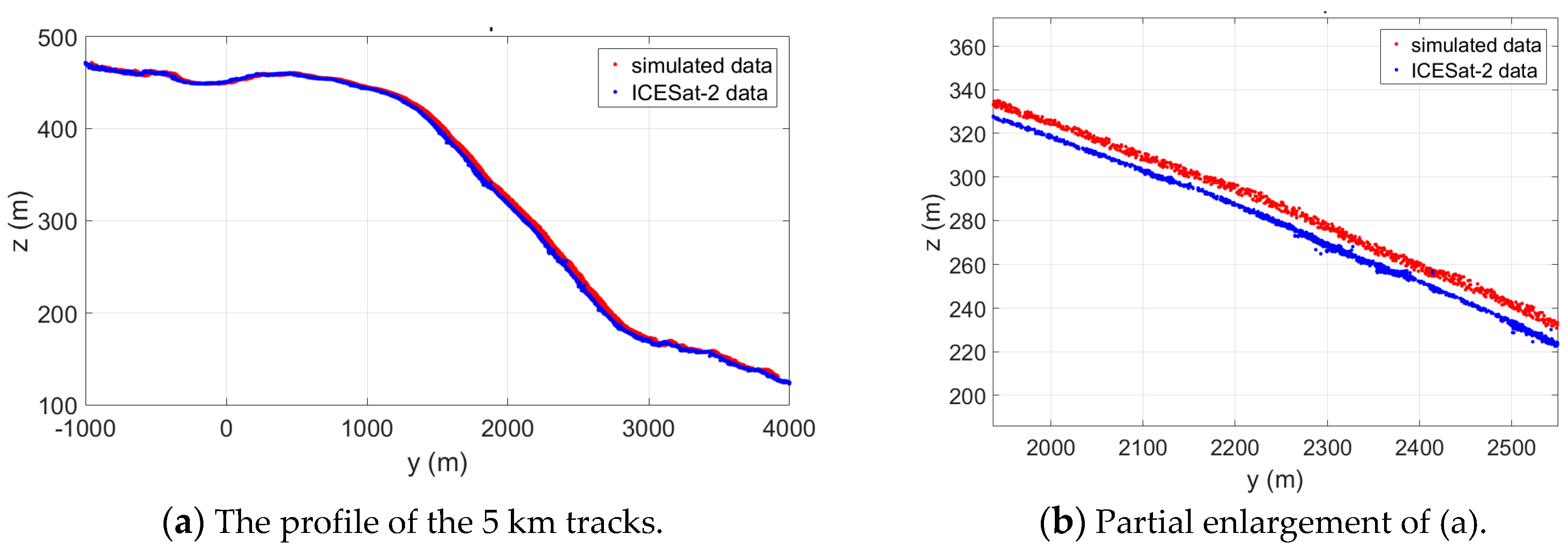
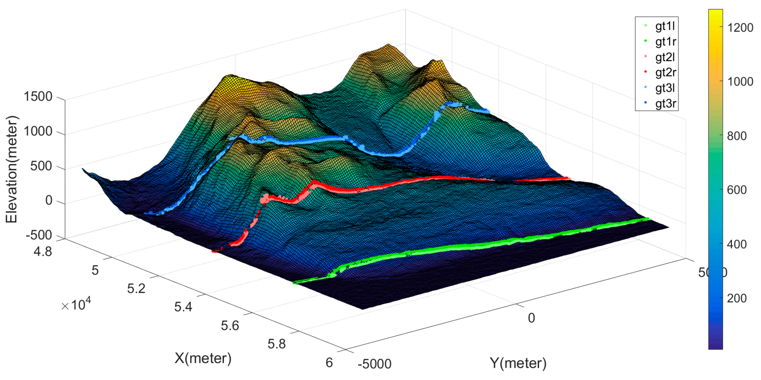
(3) The ICESat-2 data. The ICESat-2 data surveyed near McMurdo Dry Valleys on 2 November 2018 [34] were used in this paper. The Track ID is 534. The ground tracks of the data are shown in Figure 4, which contain three pairs of footprints. gt3r, gt2r and gt1r are the strong beams, whose energy is about four times that of the weak beams.

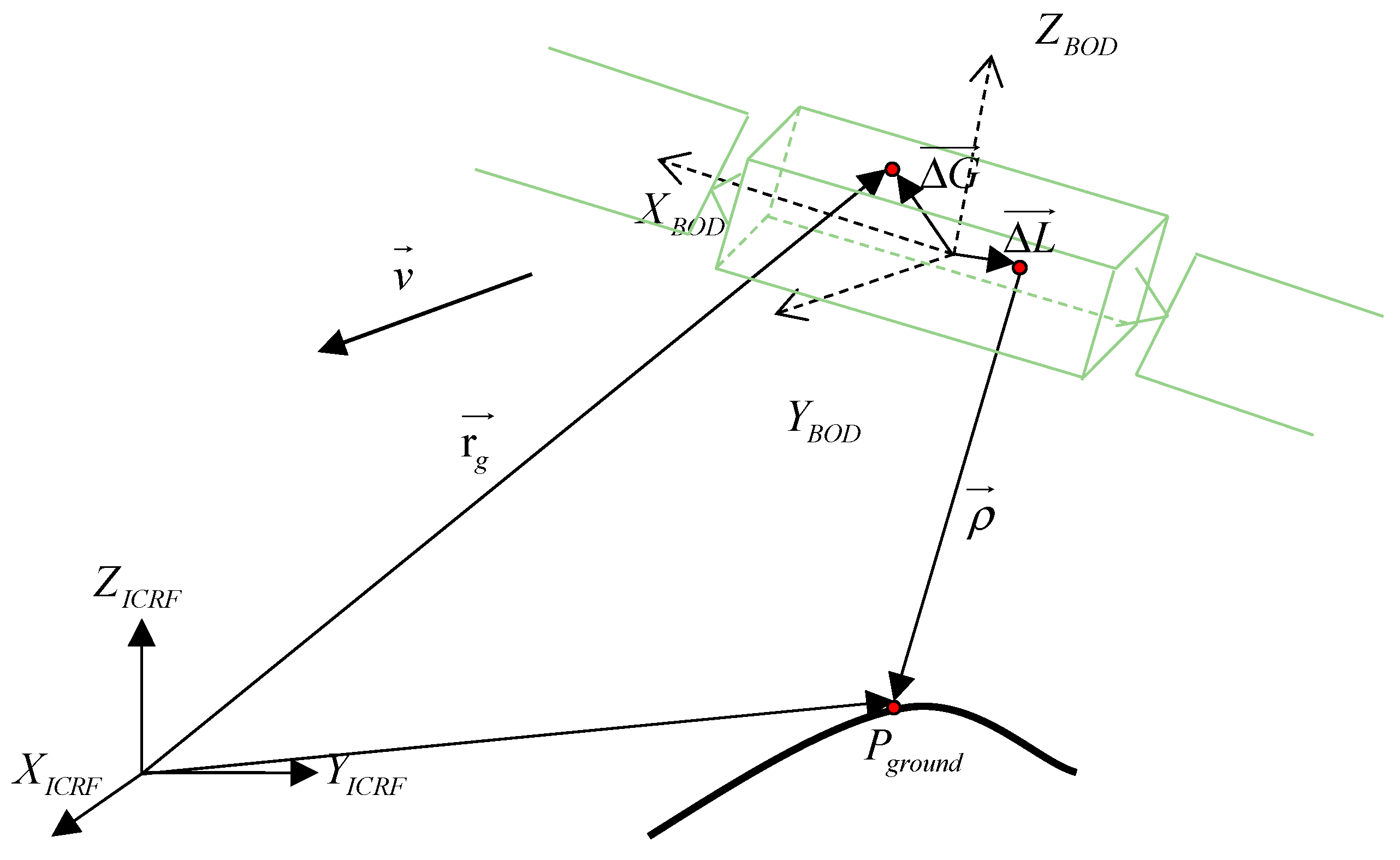
2.2. Pointing Angle Error Geometric Model

A geometric model of the spaceborne laser altimeter [25,35] is shown in Figure 5. Within this model,   ( O X Y Z ) B O D is the coordinate system of the satellite body, Δ G is the offset of the GPS antenna in the satellite body coordinate, Δ L is the laser fire point in the satellite coordinate, ( O X Y Z ) I C R F represents the international celestial reference frame (ICRF) coordinate system, r g is the position vector of the GPS antenna, v is the velocity direction and ρ 
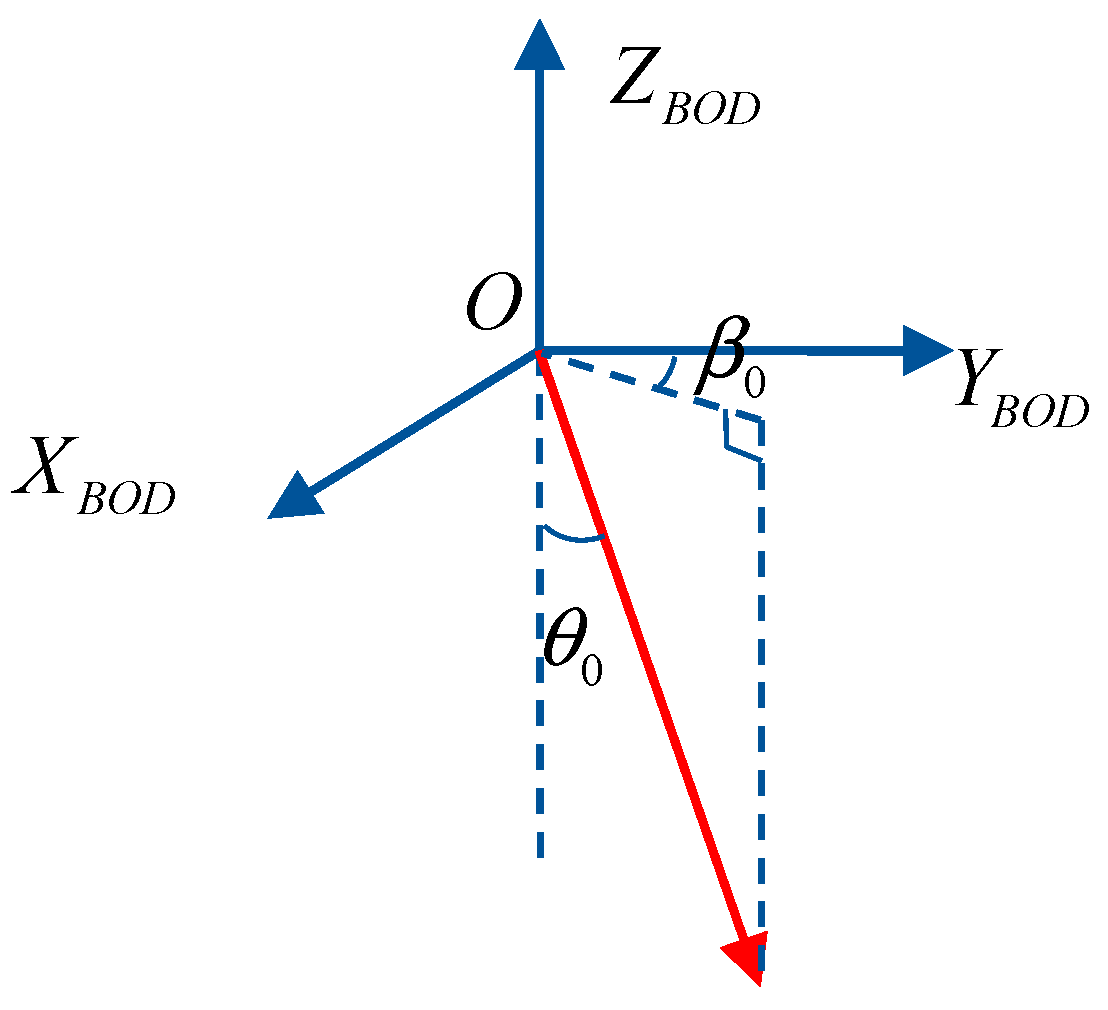
is the direction vector of the laser boresight. The relationship between the laser boresight and the satellite body coordinate system is defined in Figure 6, where θ 0 is the angle between the laser boresight and − Z B O D direction, and β 0 is the angle between the projection direction of the laser boresight on plane ( O X Y ) B O D and the Y B O D axis. ( X p , Y p , Z p ) T I T R F is the geolocation of the laser footprint in the international terrestrial reference frame (ITRF), which can be expressed by Formula (1).
[ X p Y p Z p ] I T R F = [ X s Y s Z s ] I T R F + R I C R F I T R F R B O D I C R F [ ( Δ X L Δ Y L Δ Z L ) B O D + ρ 0 ( t ) ( sin θ 0 sin β 0 sin θ 0 cos β 0 cos θ 0 ) B O D ]
where ( X s , Y s , Z s ) T I T R F is the satellite centroid coordinates in the ITRF coordinate, R B O D I C R F is the rotation matrix from the satellite coordinate system to the ICRF coordinate system, R I C R F I T R F is the conversion matrix from the ICRF coordinate system to the ITRF coordinate system, ( Δ X L , Δ Y L , Δ Z L ) T B O D is the position of the laser fire point in the satellite coordinate system. ρ 0 ( t ) is the range measured by the laser system and ( sin θ 0 sin β 0 , sin θ 0 cos β 0 , cos θ 0 ) B O D T is the laser boresight vector in the satellite coordinate.
Due to the existence of systemic errors, the estimated footprint geolocation ( X p , Y p , Z p ) T I T R F is expressed as Formula (2) [25].
[ X p Y p Z p ] I T R F = [ X s + Δ X s Y s + Δ Y s Z s + Δ Z s ] I T R F + R I C R F I T R F R B O D I C R F [ ( Δ X L Δ Y L Δ Z L ) B O D + [ ρ 0 ( t ) + ρ s y + ρ o t ] ( sin ( θ ) sin ( β ) sin ( θ ) cos ( β ) cos ( θ ) ) B O D ]
where ( Δ X s , Δ Y s , Δ Z s ) T I T R F are the position errors of the spacecraft; ρ s y is the system error including time synchronization, hardware measurement errors and other system errors; and ρ ot is the other error, which is mainly composed of atmospheric delay and tidal errors. ( θ , β ) is the estimated pointing angle with errors.
{ θ = θ 0 + Δ θ β = β 0 + Δ β
Because the spacecraft position errors [ Δ X s , Δ Y s , Δ Z s ] T can be calibrated through the ground observation station, the deviation of ( X p , Y p , Z p ) T I T R F from the actual position ( X P , Y P , Z P ) T I T R F can be calculated by Formula (4).
[ Δ X p Δ Y p Δ Z p ] I T R F = [ X p Y p Z p ] I T R F [ X p Y p Z p ] I T R F = R I C R F I T R F R B O D I C R F [ ( ρ 0 ( t ) + ρ s y + ρ o t ) [ ( sin θ sin β sin θ cos β cos θ ) ( sin θ 0 sin β 0 sin θ 0 cos β 0 cos θ 0 ) ] B O D ]
As can be seen from Formula (4), the pointing errors of θ and β will lead to a geolocation error of the footprints. To ensure the geolocation accuracy of footprints, ICESat requires a pointing accuracy of less than 1.5 arc-seconds, and ICESat-2 requires a pointing knowledge of less than 6.5 m (~2.6 arc-seconds).

2.3. Iterative Pointing Angle Calibration Method

The laser pointing angle calibration method based on terrain is used to obtain the actual pointing angles ( θ 0 , β 0 ) from the estimated angles ( θ , β ) through terrain matching. The proposed iterative least z-difference (I-LZD) algorithm is based on the least z-difference matching criterion and the least-squares matching theory [36,37]. The I-LZD algorithm is similar to the iterative method used in geomagnetic matching [38] and to the iterative calibration method used in the ICESat range and mounting bias estimation method based on a surface fitting strategy [23]. The principle of the I-LZD algorithm is described as follows.
Generally, the systematic errors ( Δ θ , Δ β ) are small, and the actual pointing angles ( θ 0 , β 0 ) can be approximately expressed by the estimated angles ( θ , β ) using Formula (5).
( ρ 0 ( t ) + Δ ρ ) ( sin θ 0 sin β 0 sin θ 0 cos β 0 cos θ 0 ) ( ρ 0 ( t ) + Δ ρ ) ( [ sin ( θ ) Δ θ cos ( θ ) + O 2 ] [ sin ( β ) Δ β cos ( β ) + O 2 ] [ sin ( θ ) Δ θ cos ( θ ) + O 2 ] [ cos ( β ) + Δ β sin ( β ) + O 2 ] cos ( θ ) Δ θ sin ( θ ) + O 2 )
where Δ ρ = ρ s y + ρ o t . After higher-order terms are ignored, we can obtain Formula (6).
( ρ 0 ( t ) + Δ ρ ) ( sin θ 0 sin β 0 sin θ 0 cos β 0 cos θ 0 ) ( ρ 0 ( t ) + Δ ρ ) [ ( sin ( θ ) sin ( β ) sin ( θ ) cos ( β ) cos ( θ ) ) + ( Δ β sin ( θ ) cos ( β ) Δ θ cos ( θ ) sin ( β ) Δ β sin ( θ ) sin ( β ) Δ θ cos ( θ ) cos ( β ) Δ θ sin ( θ ) ) ]
According to Formulas (4) and (6), the corresponding deviation between ( X p , Y p , Z p ) T I T R F and ( X p , Y p , Z p ) T I T R F can be expressed by Formula (7).
[ Δ X p Δ Y p Δ Z p ] I T R F = [ X p Y p Z p ] I T R F [ X p Y p Z p ] I T R F = R I C R F I T R F R B O D I C R F [ ( ρ 0 ( t ) + Δ ρ ) ( Δ β sin ( θ ) cos ( β ) + Δ θ cos ( θ ) sin ( β ) Δ β sin ( θ ) sin ( β ) + Δ θ cos ( θ ) cos ( β ) Δ θ sin ( θ ) ) B O D ]
On the other hand, for a given terrain, let h ( X p , Y p ) be the elevation of the horizontal coordinates ( X p , Y p ) , which corresponds to the laser footprint ( X p , Y p , Z p ) T I T R F . Similarly, let h ( X p , Y p ) be the elevation of coordinates ( X p , Y p ) . Based on the gradient information of the terrain, for a given ( Δ X p , Δ Y p ) , h ( X p , Y p ) can be approximated by h ( X p , Y p ) using Formula (8).
h ( X p , Y p ) h ( X p , Y p ) h x ( X p , Y p ) Δ X P h y ( X p , Y p ) Δ Y P
where h x ( X p , Y p ) and h y ( X p , Y p )  are the gradients in the x and y directions for point ( X p , Y p , h ( X p , Y p ) ) T I T R F in the terrain. According to Formulas (7) and (8), the z-difference between the actual footprints and their corresponding terrain can be derived from Formula (9).
Δ v = Z P h ( X p , Y p ) Z P Δ Z P h ( X p , Y p ) + h x ( X p , Y p ) Δ X P + h y ( X p , Y p ) Δ Y P
According to the least square theory, we can obtain the target Equation (10).
i = 1 N ( Δ v i ) 2 = m i n
Normally, let i = 1 N ( Δ v i ) 2 respectively take the partial derivatives of Δ θ , Δ β and Δ ρ , and the equation group can be obtained by setting these partial derivatives to zero. By solving for Δ θ , Δ β and Δ ρ , the one-step approximation to the actual angles ( θ 0 , β 0 ) from the known angles ( θ , β ) can be obtained. The pointing angles and ranging offsets can be precisely calibrated by several iterations. Considering the complexity of solving the above equation group, we decompose the above one iteration into two steps.
Step 1: Updating ( θ 0 , β 0 ) : Keeping Δ ρ constant, the updates of Δ θ and Δ β can be achieved by solving Equation group (11). Then, ( θ 0 , β 0 ) can be updated by Formula (3).
{ [ i = 1 N ( Δ v i ) 2 ] ( Δ θ ) = 0 [ i = 1 N ( Δ v i ) 2 ] ( Δ β ) = 0
Step 2: Updating ρ 0 : When the pointing angle ( θ 0 , β 0 ) is constant, Formula (9) becomes Δ v = Z P h ( X p , Y p ) . Then, the update of ρ 0 can be achieved by solving Equation (12).
[ i = 1 N ( Δ v i ) 2 ] ( Δ ρ ) = 0
The result of the above two steps is the formation of one-step corrections to the values of θ 0 , β 0 and ρ 0 . Due to the approximate errors in the calculations, iterations are required to obtain an accurate correction.

3. Results

We designed four experiments to verify the advantages and limitations of our method. The experimental objectives were as follows: (1) Comparison of the I-LZD and pyramid least z-difference algorithm (P-LZD) algorithms; (2) showing the effect of footprint length on the calibration results; (3) showing the off-nadir pointing’s impact on the calibration results; and (4) verifying the effectiveness of our method on the ICESat-2 data.

3.1. Comparison of Calibration Methods

In this experiment, simulated spaceborne photon-counting data with lengths of 1 km and 2.5 km were used to calibrate the pointing angles using our I-LZD method and the widely known pyramid least z-difference algorithm (P-LZD) [20,35], respectively. The P-LZD method adopts the coarse-to-fine search strategy. Let Δ θ and Δ β Δ β be the pointing angle errors. The P-LZD method finds these errors by traversing the possible parameter space of Δ θ and Δ β with different ranges and intervals. At the beginning, it searches the parameter space with a relatively large range and interval, and the offset possessing the least z-difference can be found. Then, based on the known offset, the P-LZD method re-searches the parameter space with a smaller range and interval. After several iterations, Δ θ and Δ β can be precisely found. The I-LZD method also searches for Δ θ and Δ β in the parameter space. The difference is that it has no fixed search range and interval; it iterates in the direction that makes the Z-difference smaller. The I-LZD method stops calculation if the number of iterations exceeds 30, or if the correction value in each iteration is less than 0.01 arc-seconds. Other simulation parameters are listed in Table 2.
The initial search range was set to be ± 64 for Δ θ and ± 512 for Δ β . The search interval of each layer was a quarter of the search range. The search range of the next layer is half of the previous one. The number of iterations is set to be 10, resulting in a resolution of 0.0625 for Δ θ and 0.5 for Δ β . Since the referenced P-LZD method only searches the parameter space of θ and β , here we compared the calibration results of the P-LZD method and our I-LZD method with no range error. The results are shown in Figure 7 and Figure 8.
As can be seen from Figure 7a, when 1 km length tracks are used, the calibration error of θ is ~0.3 arc-seconds for the I-LZD algorithm, corresponding to a geolocation error of ~0.7 m. Moreover, the calibration results change little with different initial errors of θ and β. For the P-LZD algorithm, most of the calibration errors are better than the I-LZD algorithm. However, its calibration errors vary greatly with the initial errors of θ and β. Figure 8 shows the result when 2.5 km length tracks are used. The calibration result of θ is below 0.05 arc-seconds for the I-LZD algorithm, corresponding to a geolocation error of ~0.1 m. At the same time, its calibration results maintain good consistency with different initial errors. For the P-LZD algorithm, the calibration errors are slightly lower than the result when 1 km length tracks were used. Meanwhile, its calibration errors still fluctuate with different initial errors.
For the calibration result of β, the errors of the I-LZD method and the P-LZD method are both large, and they are not effectively calibrated under the current experimental conditions. The main reason for this is that under the current experimental parameters ( θ 0 = 100 arc-seconds), angle β has little impact on the geolocation of footprints, which is mainly determined by the angle θ. In addition, the calibration time of the I-LZD method is only 1/5 to 1/8 of that of P-LZD, which can be seen in Figure 9.
Due to the influence of the atmosphere, the ranging delay correction is typically between −2.6 and −0.9 m, depending on the atmospheric state [10]. A total range error of 50 cm was assumed in our simulation, and the I-LZD method was used to calibrate the pointing angle and range error. The result is shown in Figure 10.
As can be seen from Figure 10, with an initial range error of 50 cm, the calibration error of the pointing angle is close to 1.5 arc-seconds, corresponding to ~3.6 m of position offset, if the range error is not corrected. When the ranging error is corrected, the calibration error can be reduced to about 0.35 arc-seconds, corresponding to ~0.8 m of position offset, which is comparable to the calibration result without ranging error in Figure 7. Meanwhile, the ranging error can be corrected to below 3.5 cm with an average of ~2 cm. The range errors are shown in Figure 11.
The experimental results of this section show that the I-LZD method has better calibration stability and shorter calibration time than the P-LZD method. At the same time, our method can also effectively calibrate the pointing angle when the range error exists. Meanwhile, simulation results using 1 km and 2.5 km lengths of track show that the I-LZD method is significantly affected by track length.

3.2. Influence of Track Length

In order to further determine the influence of track length, tracks with different lengths ranging from 20 to 5000 m are used for calibration. Detailed parameters are listed in Table 3.
The tracks with different lengths were derived from a track with a total length of 5 km, which is shown in Figure 12. All tracks have the same starting point but different ending points. A total of 18 segments of data were intercepted, ranging from 20 to 5000 m.
As can be seen from Figure 13, the calibration errors of β and θ decrease rapidly with the increase in track length. The calibration errors of θ can be reduced to less than 1 arc-second when a 100 m long track was used. When a 2500 m long track was used, the calibration error is close to 0.01 arc-seconds. For the β angle, although the calibration errors decrease with the increase in track length, there are still hundreds of arc-seconds of errors. Further methods should be applied to reduce its calibration errors.

3.3. Calibration with Off-Nadir Pointing

In order to further reduce the calibration error of β, we studied the influence of off-nadir pointing on the pointing angle calibration. The idea comes from the observation that when the pointing angle θ is small, β has little impact on the position of footprints, and this may limit the calibration accuracy of β. The off-nadir pointing could be either a specialized spacecraft maneuver or the planed off-track pointing in the ICESat-2 mission, in which ICESat-2 will be off-nadir pointed from the reference ground track to further improve the longitudinal spatial sampling. The experimental parameters are listed in Table 4.
As can be seen from Figure 14, with the increase in the off-nadir pointing angle, the calibration errors of β angle decrease rapidly, and when the off-nadir pointing angle is 5°, the calibration error is about 2 arc-seconds. However, the calibration errors of θ do not decrease significantly. The above phenomenon can be explained by the geometric model of measurement. The influence of β on footprint positioning is based on θ0. When θ0 is small, the total deviation is small so the influence of β on footprint geolocation can almost be ignored. When the off-nadir angle increases, the influence of β on footprint geolocation also increases. However, for the angle θ, its influence on footprint geolocation is almost the same when off-nadir angles are less than 5°. Figure 15 shows the total geolocation errors after calibration with different off-nadir pointing angles, and these errors are still dominated by the errors of θ.

3.4. ICESat-2 Data Experiment

ICESat-2 tracks consistent with previous data were selected to verify our I-LZD calibration method, which are shown in Figure 16. The gt2r track range from −1000 to 4000 m in Figure 16 was selected as our experimental data. Signal photons were obtained by a density statistics algorithm. Considering that the main purpose of pointing angle calibration is to improve the geolocation accuracy of footprints, and the fact that when there is a small error in the pointing angle, this error will cause the deviation of footprint positions in x, y and z directions, we indirectly verify the pointing angle calibration of the I-LZD method by correcting the positioning deviation of the footprint. The positions of the original ICESat-2 footprints are taken as the true values in the experiment. Furthermore, the positioning accuracy is considered to be within the required 6.5 m. Additional deviations in the x-axis, y-axis and z-axis were added in the ICESat-2 data to simulate the deviations due to pointing angle errors. We conducted two experiments (1) to analyze the influence of track length on calibration results and (2) to verify the I-LZD algorithm by using different datasets.
(1)
Calibration using different track lengths.
ICESat-2 data ranging from 20 to 5000 m in length were used for calibration. A total of 18 datasets with different lengths were intercepted. Here, the original ICESat-2 data are used as a baseline. The tracks with errors are obtained by adding 12 m offsets in the x and y directions, respectively, and a 0.5 m offset in the z-direction. The calibration results are shown in Figure 17.
The calibration results show that when the footprint length is greater than ~300 m, the horizontal deviation after calibration tends to be stable, at about 3 m, and the corresponding pointing angle deviation is about 1.2 arc-seconds. Although the calibration error is larger than the simulation results in Section 3.2, the footprint geolocation error still meets the design requirements of ICESat-2 (6.4 m).
(2)
Calibration using multiple datasets.
In order to verify the consistency of the I-LZD method, ICESat-2 data of 5 km long are divided into five equal segments, each of which is 1 km long. Furthermore, each segment is deviated by 12 m, 12 m and 0.5 m in the x-axis, y-axis and z-axis, respectively, to simulate the deviations due to pointing angle errors. Then, the I-LZD algorithm is used to calibrate the deviations. The calibration results are shown in Table 5.
The calibration results maintain a good consistency: the horizontal offset after calibration is approximately 3 m for each segment. The errors show good consistency, being much like systematic errors. However, as the real ground footprint location is not known, the cause of this error cannot be further determined at present.

4. Discussion

Pointing angle calibration is a basic problem in the spaceborne laser altimeter. Most of the current terrain matching-based pointing angle calibration methods are for large spot and full-waveform laser altimeters, such as GLAS, or laser altimeters without waveform recording ability, such as the laser altimeter on ZY3-02 [39]. A wide range of terrain is needed in these calibrations. Considering the new characteristics of the photon-counting laser altimeter, which was launched recently, our paper explored the feasibility of pointing angle calibration using a small range of terrain, and an efficient calibration algorithm was proposed. The following is a further discussion about the novelty of our method, some interesting experimental phenomena, limitations and so on.

4.1. Comparison with Other Methods

Since there is little research found in the literature on the calibration methods for photon-counting lidar based on terrain matching, we mainly compare our calibration method with the ones used for traditional laser altimeters. The photon-counting laser altimeter has distinct characteristics compared with the traditional ones. The traditional laser altimeters usually have large spots and low repetition frequency, e.g., GLAS has a footprint diameter of about 70 m and a footprint interval of about 170 m. Meanwhile, GLAS has full waveform recording ability, which means that a large number of echo photons can be obtained within one footprint, and the decomposition of these waveforms can help toward understanding the elevation distribution [40]. However, the ATLAS of ICESat-2 has a footprint of less than 17 m with an interval of 0.7 m. Although its footprint is small, there is only a small number of echo photons, and the random error of altitude deviation in rough terrain areas is large.
Regarding the calibration methods based on terrain matching, the traditional laser altimeter mainly has two kinds of methods, which are the terrain profile matching method and the waveform matching method [41]. However, the waveform matching method is a special method for full-waveform laser altimeters, which is not suitable for photon-counting laser altimeters with only a few echo photons. The terrain profile matching method calibrates the pointing angle based on the residual error between the measured elevation and the terrain. Our method falls into the latter category. In general, our terrain profile matching strategy for small footprint interval altimeters based on a small range of terrain is similar to the strategy for large footprint intervals based on a large range of terrain. However, the measurement accuracy of photon-counting lidar does not increase proportionally. On the contrary, the photon-counting altimeter receives less information and has larger error in single footprint measurement. Therefore, a calibration method based on a small range of terrain still needs to be studied, which is also an important intention of this paper. Furthermore, regarding the calibration methods based on terrain profile matching, the most direct method is to traverse the parameter space to find the location of the minimum elevation difference. The pyramid search method has been developed after the fact to speed up the search progress [20,
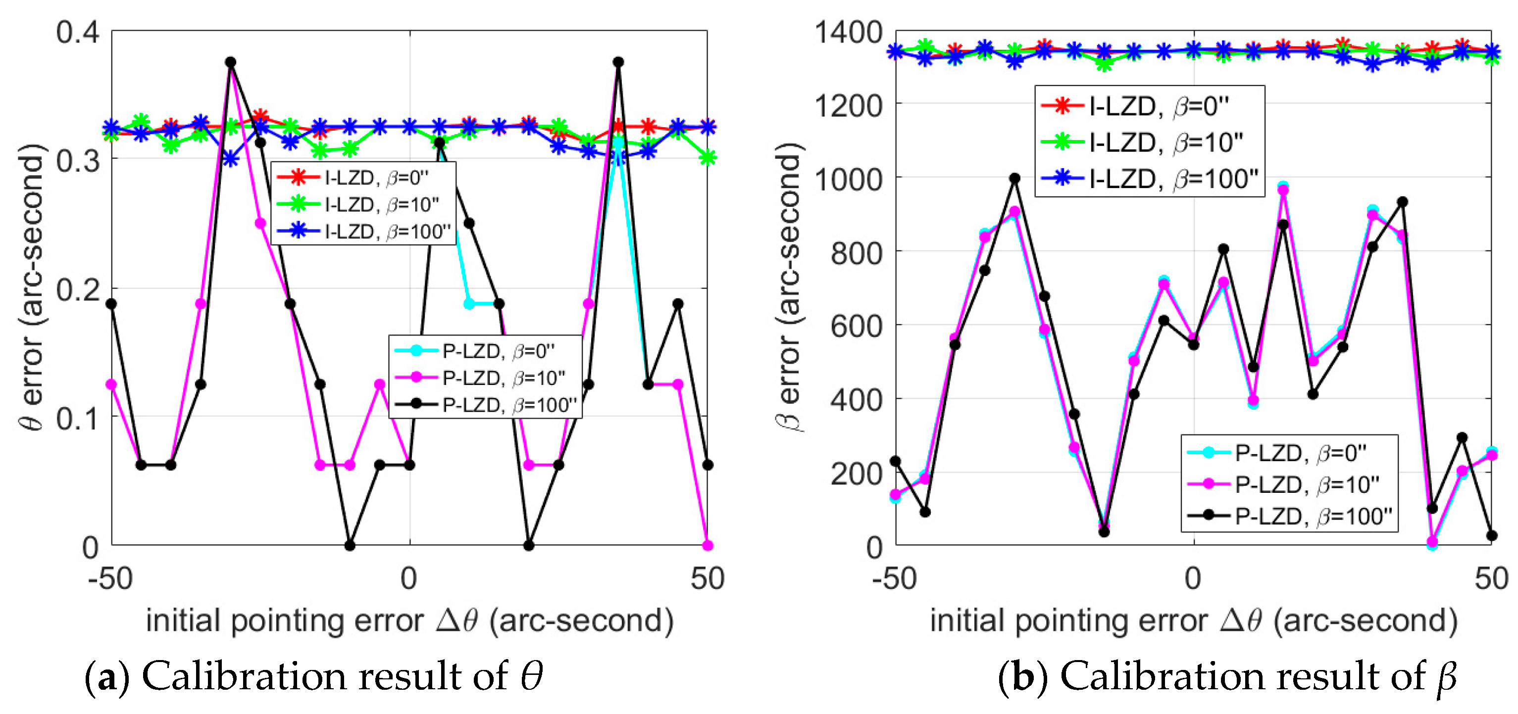
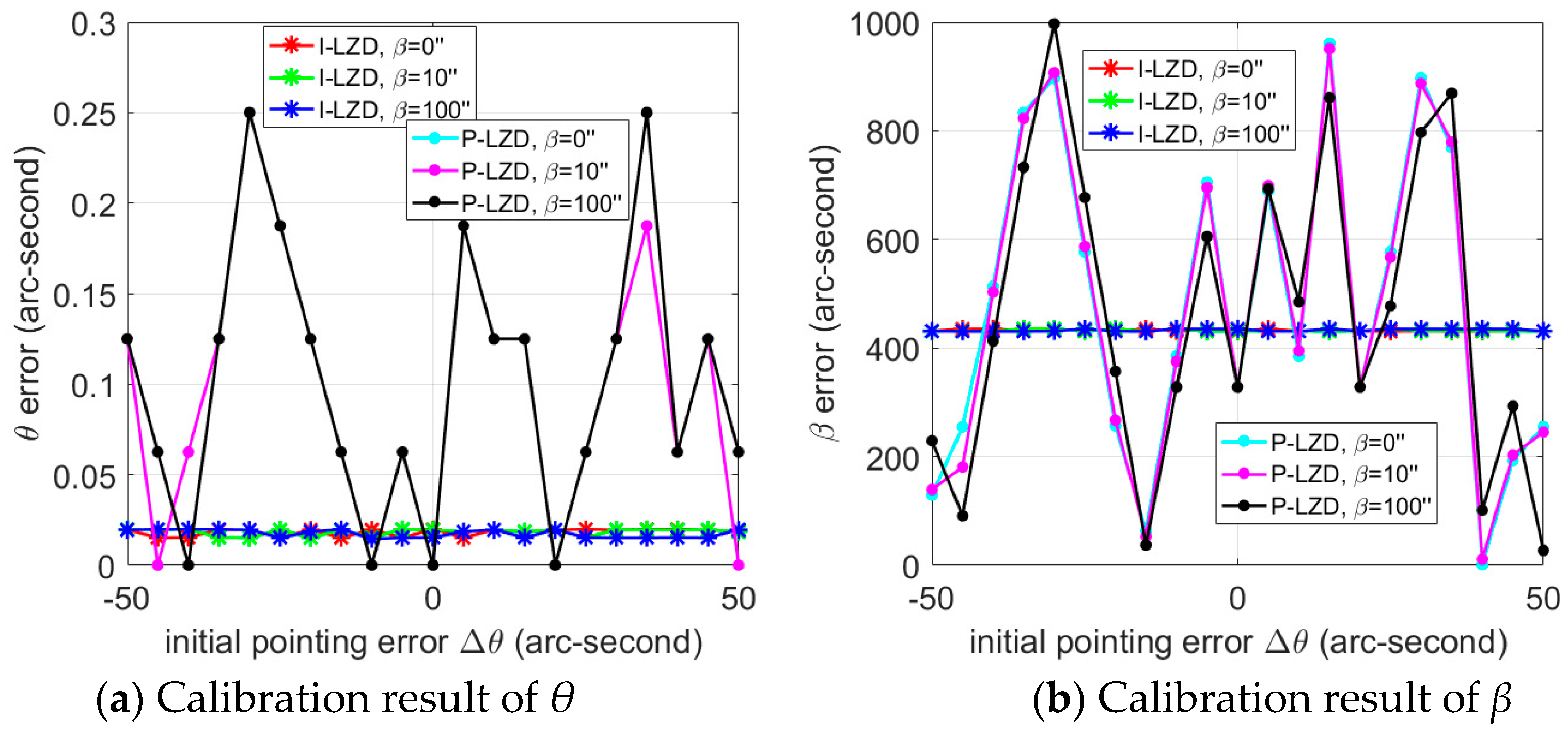
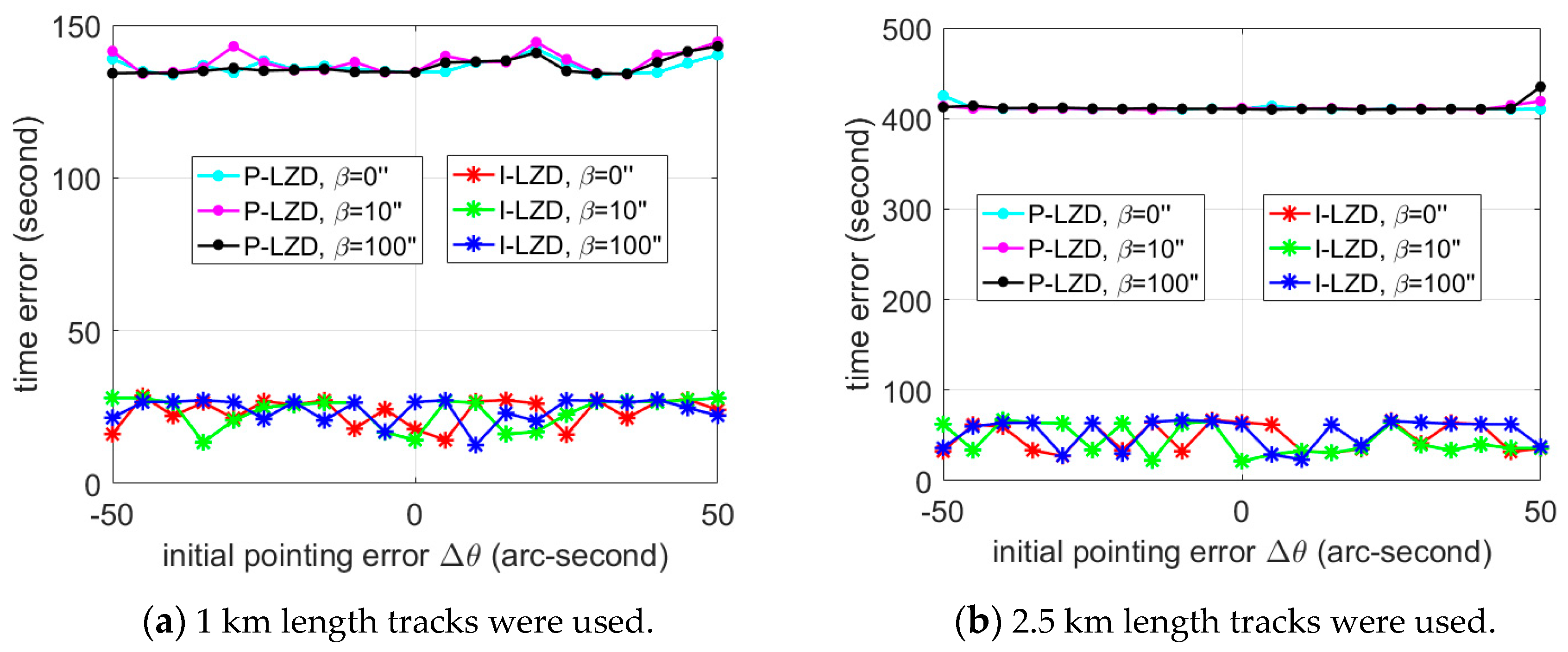
35], and it was compared in our research. Compared to our method, there are many problems in the pyramid method. Firstly, although the matching time can be greatly reduced by pyramid search compared with the direct search method, it is still relatively long compared with our iterative method, which searches along the gradient direction. Secondly, in our experimental parameter settings, the P-LZD method shows instability, as shown in Figure 7 and Figure 8. Theoretically, the P-LZD and I-LZD methods are based on the same LZD matching criteria; their final search results should be similar, and their main difference should be in their efficiency. In order to determine the different behaviors of the P-LZD and I-LZD algorithms, for the experimental data corresponding to Figure 7 and Figure 8, we traversed the parameter space of Δ θ and Δ β at an interval of 0.05 arc-seconds and 100 arc-seconds around θ 0 and β 0 . The result is shown in 
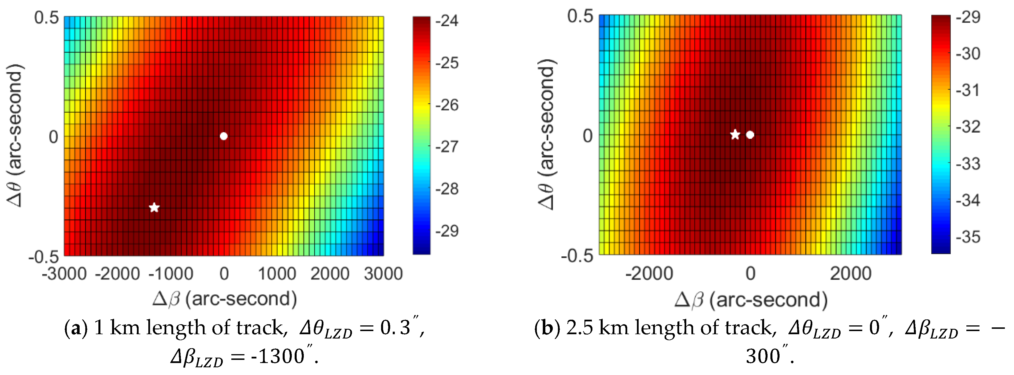
Figure 18 (the z-difference is displayed inversely).
It can be seen from Figure 18 that the least z-difference (LZD) position is ( 1300 , 0.3 ) for the 1 km long track. Meanwhile, for the 2.5 km long track, the LZD position is ( 300 , 0 ) . By comparison with the results in Figure 7 and Figure 8, the calibration results of the I-LZD method are closer to the actual position. For the P-LZD method, the actual LZD position of the 1 km long track is beyond its search range, and this may lead to the optimistic result in Figure 7. The actual LZD position of the 2.5 km track is within the search range of the P-LZD method; however, the result of the P-LZD method still shows the characteristic of fluctuation. Therefore, the search parameters of the P-LZD method need to be well estimated in advance to balance calculation time and effect. However, there is no need for prior parameter estimation in the I-LZD method.
In addition, a similar iterative terrain matching method was proposed in reference [41] for the calibration of full-waveform laser altimeters. However, this method required the calculation of the normal vector of terrain over the footprint region, being compulsory to carry out a local plane fitting of the terrain. On the contrary, our method is based on the gradient of the terrain, so no plane fitting is needed. At the same time, in the idea of algorithm modeling, the method in [41] focuses on building a functional relationship between laser ranging and pointing angles using terrain information, while our method focuses on establishing the approximate relationship between the error value and the truth-value.

4.2. Factors Influencing Calibration Accuracy

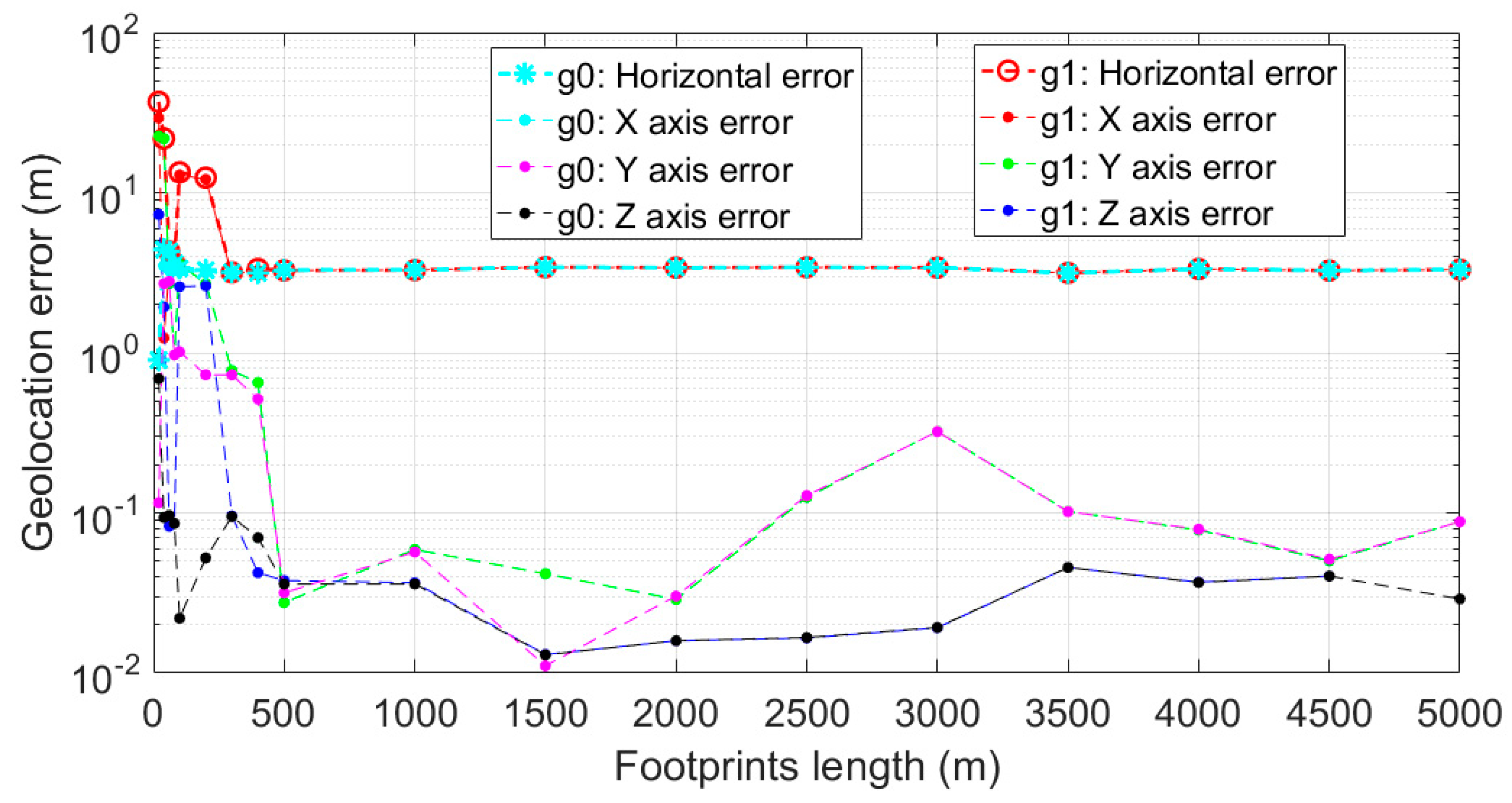
(1) The influence of footprint length.
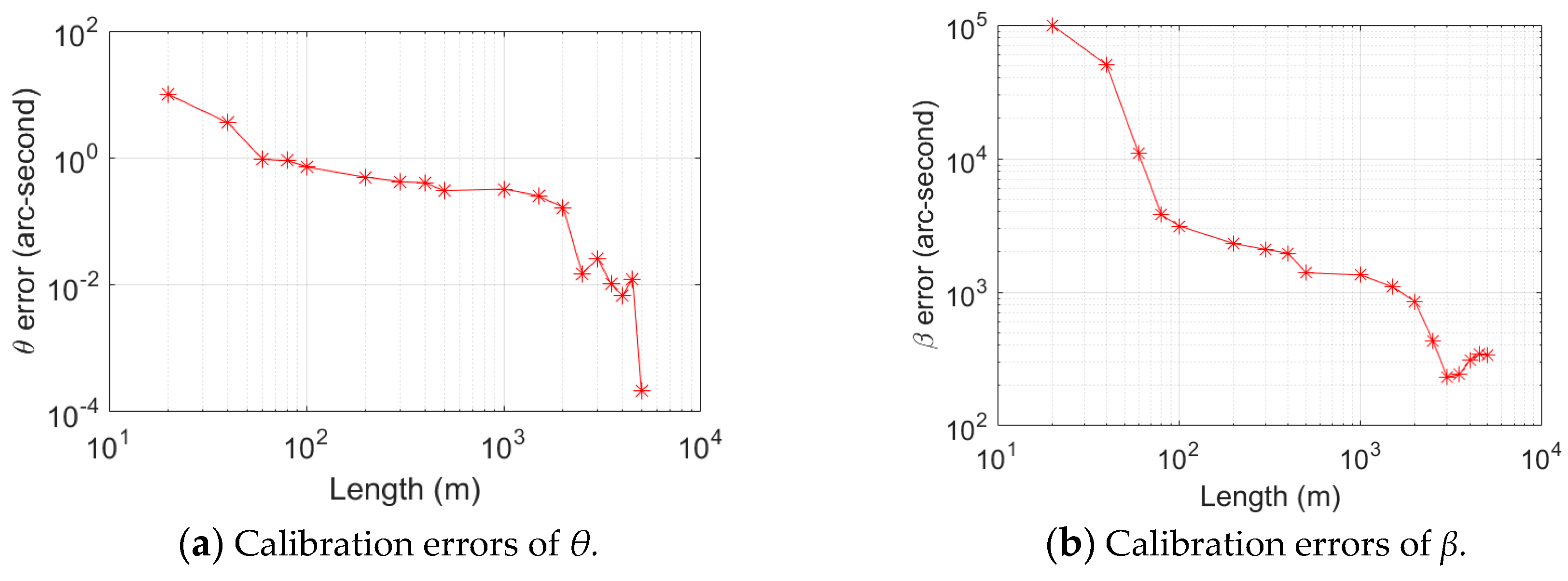
The results in Figure 7 and Figure 8 and Figure 13 and Figure 14 show that the calibration results are affected by the lengths of footprints. When the data length is less than 100 m, the calibration error is close to or greater than one arc-second. When the data length is more than 1 km, the calibration error can be reduced to less than one arc-second. Using shorter data lengths helps to expand the range of terrain options. However, when the data length is short, the influence of a single range error of the photon-counting lidar may increase. When a single measurement value is used to calibrate the pointing angle, Formula (13) can be used to estimate the influence of range error on the pointing angle [19]. For a 1° slope (S) and 500 km orbit (h), a range error of 0.5 m will cause a θ error of ~10 arc-seconds. However, increasing the number of equal precision measurements can usually improve the ranging precision.
σ θ = cos ( θ + S ) h tan ( θ + S ) σ ρ
As we can see from Figure 18, with the increase in data length, the actual LZD position is closer to the theoretical position. We can further analyze the factors that affect the precision of the calibration result by the error model. Formula (9) can be viewed as a function of Δ β and Δ θ as follows.
Δ v i = l i + Δ β k β i + Δ θ k θ i
where i is the footprint number and l i = Z p i h ( X p i , Y p i ) . li represents the matching error of laser footprints and terrain. Let σ 0 , σ β and σ θ be the precisions of l i , Δ β and Δ θ , respectively. Their relationship can be derived from the error theory as follows.
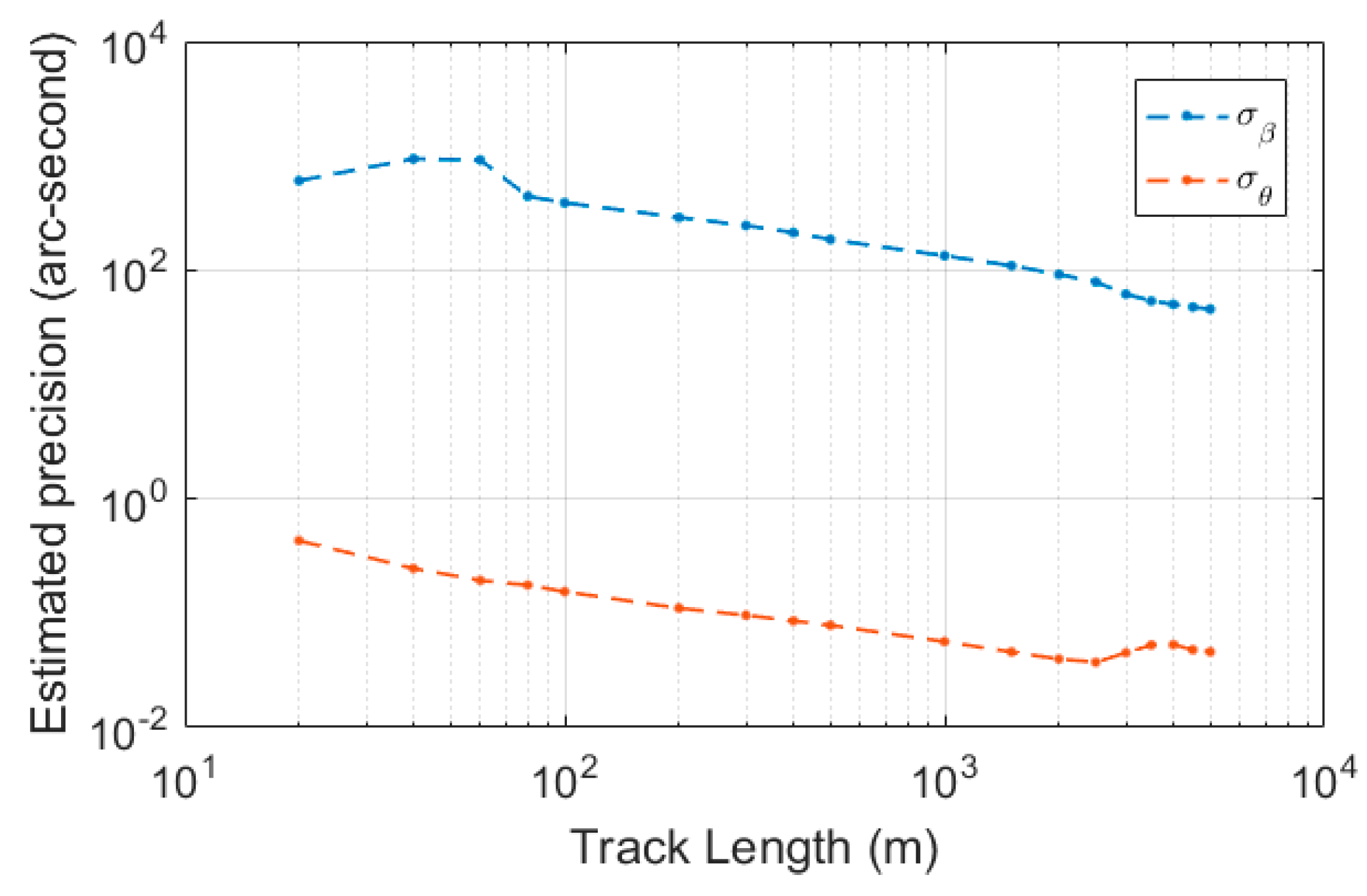
{ σ θ = λ i = 1 n k β i 2 σ 0 σ β = λ i = 1 n k θ i 2 σ 0 λ = 1 1 ( i = 1 n k θ i k β i ) 2 i = 1 n k θ i 2 i = 1 n k β i 2 ,
where
{ k β i = Δ v i Δ β k θ i = Δ v i Δ θ .
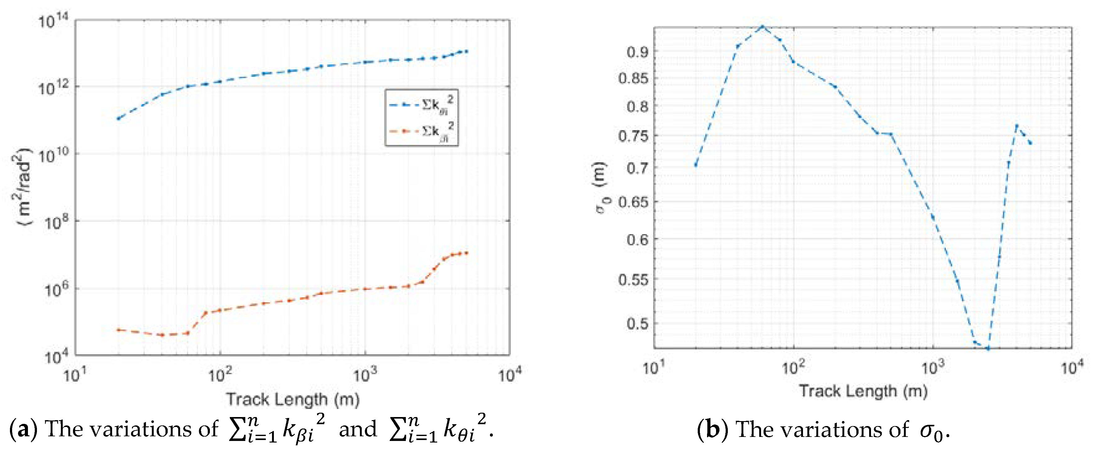
Figure 19 shows the estimated precisions based on the above error model under different track lengths; the terrain data and altimeter data from the experiment were used. In addition, Figure 20 shows the variation of i = 1 n k β i 2 , i = 1 n k θ i 2 and σ 0 with different track lengths.
Figure 19 and Figure 20 show the factors that influence the calibration. Because λ 1 in the experiment, it is not shown in the figure. Firstly, with the increase in track length, the estimated precision gradually decreases with the length. Secondly, the precision of β is about three orders of magnitude lower than that of θ . Thirdly, among all the factors, i = 1 n k β i 2 and i = 1 n k θ i 2 vary in a larger range, and their tendencies are consistent with the estimation precision. In the satellite coordinates, k β i and k θ i could be represented as follows.
{ k β i = h x i ρ i cos β sin θ h y i ρ i sin β sin θ k θ i = h x i ρ i sin β cos θ + h y i ρ i cos β cos θ ρ i sin θ
where ρ i is the laser range, and h x i and h y i are the gradients in x-direction and y-direction for footprint i. It can be seen that the terrain variations have a great impact on k β i and k θ i . When the terrain is flat, k β i   =   0 , and β cannot be calibrated by terrain matching. In general, i = 1 n k β i 2 and i = 1 n k θ i 2 will increase with the track length. However, their increased amplitudes also depend on the correlations among h x i , h y i and the pointing angles. This may lead to an optimal terrain selection problem.
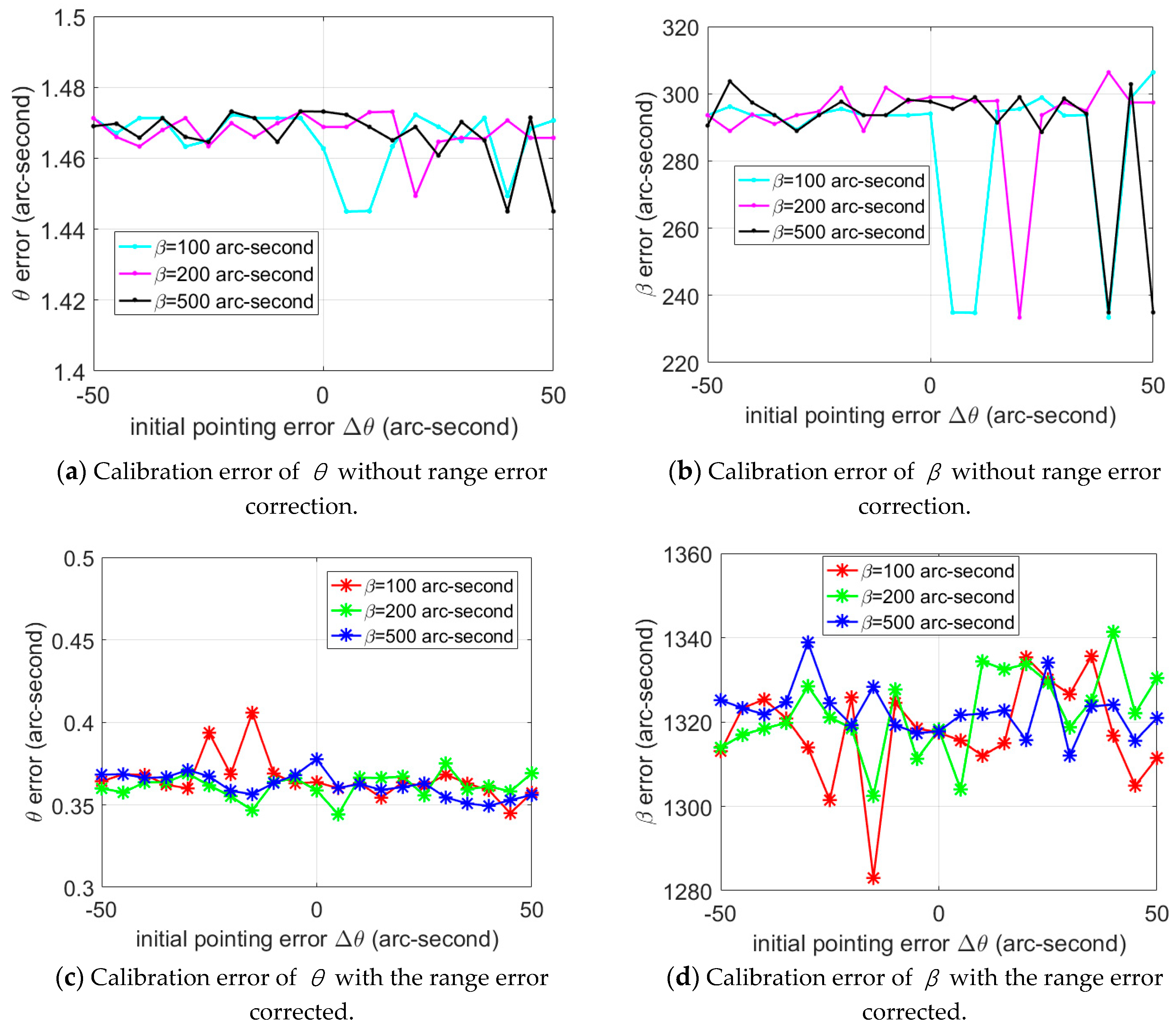
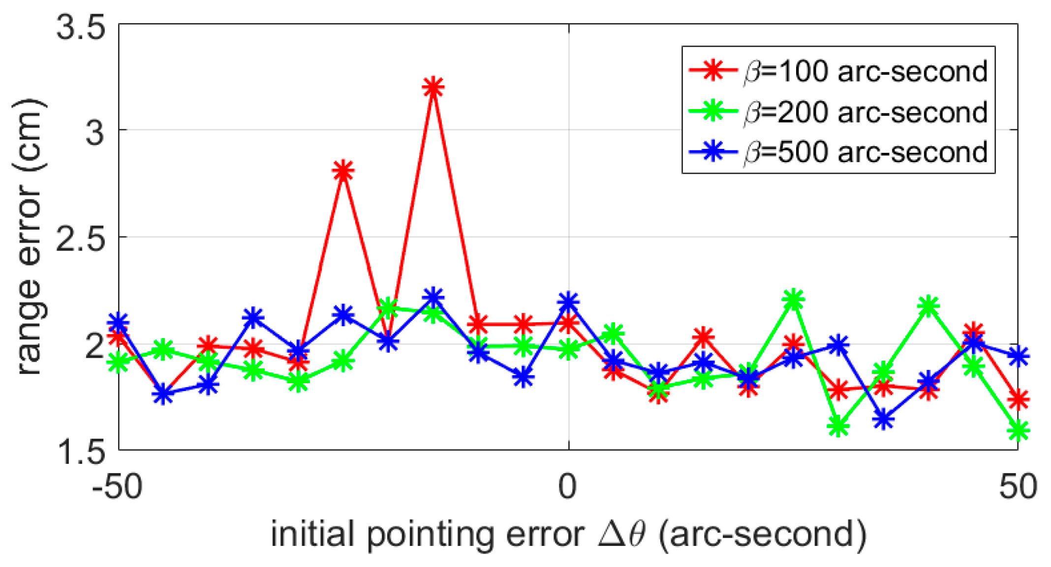
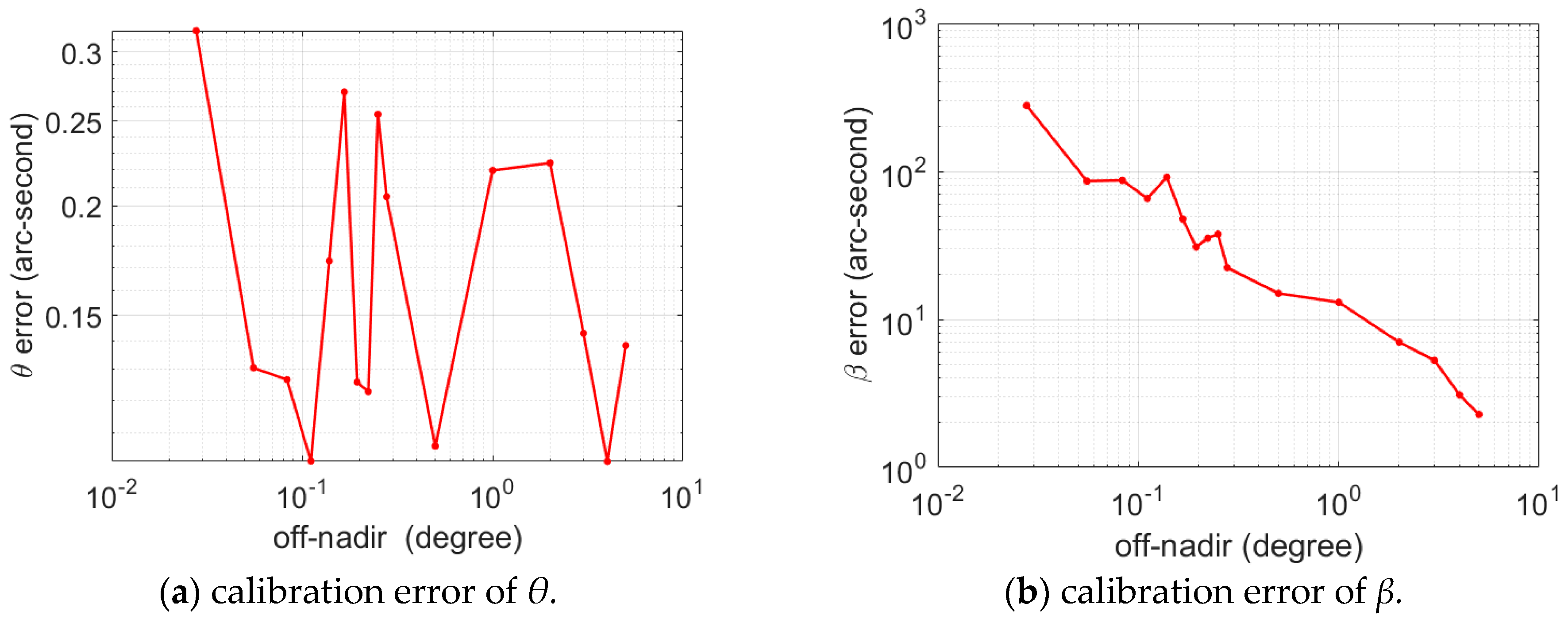
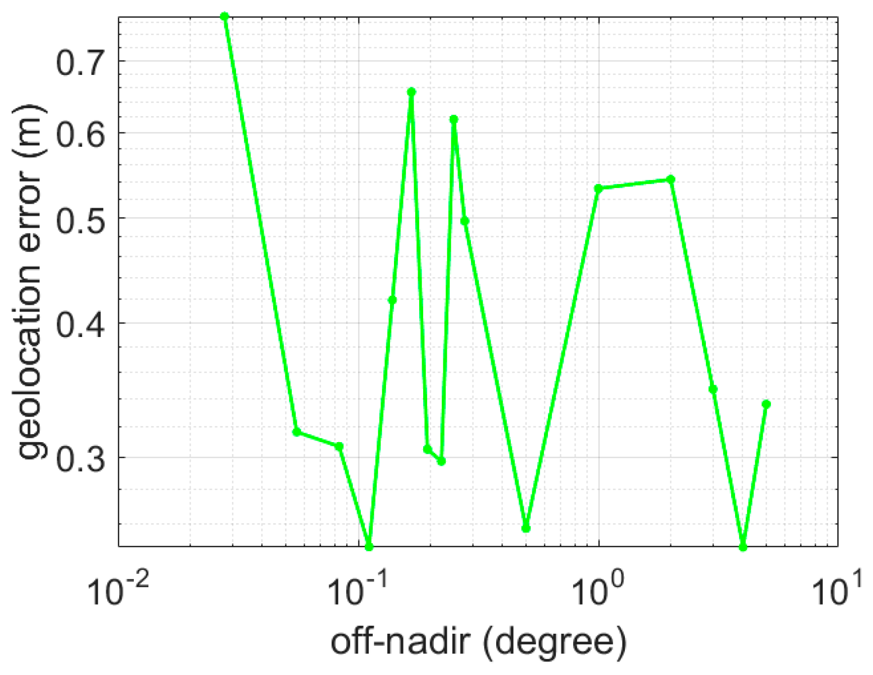
(2) The influence of off-nadir pointing.
The results of experiment 3.3 indicate that with the increase in the off-nadir pointing angle, the calibration accuracy of β increases rapidly, but the calibration accuracy of θ angle shows little change. According to the measurement geometry model, we can easily see that when the θ angle is small (such as 100 arc-seconds), the β angle has little influence on the position of footprints. However, with the increase in the off-nadir pointing angle, the influence of β angle on the footprint position also increases. Because we adopt the calibration criterion based on minimum elevation difference, the calibration accuracy of parameters depends largely on their influence on the elevation difference. This can explain why the calibration accuracy of β angle increases with the off-nadir angle.

4.3. Limitations of Our Calibration Method

Convergence to local optimality: Since our algorithm approximates to the local optimum in each iteration, it will face the problem of convergence to the local optimum. For this problem, we need to take measures to make the iteration process jump out of the local optimum. A coarse-to-fine strategy of a hierarchical representation of the terrain can be used to limit the sensitivity to local surface variations, and this method can enhance the rate of convergence [23]. In addition, for the case of large initial angle error, large-range DEM [16] data can be used as the matching terrain for a rough search. Meanwhile, correlation matching criteria can also be considered for its large pull-in range, which is often used in image matching [42]. The Monte Carlo method used in [23] can also be used to find the global optimal location.
The influence of spacecraft attitude error: In our algorithm, there is no special treatment for the attitude measurement error of the spacecraft. In fact, the attitude measurement error of the star sensor will be absorbed into the errors of θ and β. Therefore, their influence will be corrected indirectly.
The influence of topographic changes: The precondition of our method is the accurately measured terrain. Considering that the calibration may be carried out throughout the entire mission of the spaceborne altimeter, which may last for several years, the influence of the terrain modifications between airborne and spaceborne acquisitions needs further study. In addition to selecting almost constant areas as matching terrain, we can also improve the practical value of the algorithm in relation to two aspects. (1) Extracting the parts of the terrain that remain unchanged. For vegetation-covered areas, we can extract the ground through appropriate algorithms to obtain a relatively stable terrain from both airborne and spaceborne acquisitions; (2) Detecting the modifications. The terrain to be matched can be segmented, and the matched offset of each segment can be evaluated separately; then, the segments that may have changed can be removed by statistical methods. At the same time, because our algorithm only needs a short track, some man-made structures with little change, such as a region where buildings are relatively constant in the city, can also be used as a candidate for matching terrain. Calibration methods based on these terrains still need to be further validated.

4.4. Experimental Limitations

In our experiment, there are still some limitations: (1) Although there was a random deviation of several meters between the simulation footprints and the actual elevation, the real photon-counting lidar measurement results also contain a large amount of background noise, and noise filtering is still a big challenge [43,44,45]. (2) In addition, in our simulation, the change in target reflectivity within the footprint is not considered. The basic assumption of the simulation algorithm is that the detection probability of the echo signal in the footprint is the same, or the detection probability of each position in all the footprints is the same. However, when the track is short, the reflectivity may be non-uniform or deviate in a certain direction, which will affect our simulation method. (3) The point cloud density of airborne lidar used in our experiment was not high enough. The point cloud density and its uniformity will also affect the randomness of the footprint simulation. In the case of off-nadir pointing, the effect of refraction needs to be considered. Atmospheric refraction is assumed to delay the roundtrip measurement with no effect on the laser spot location. This effect is expected to be small for the nadir-looking but may be significant for off-nadir operations.

4.5. Applications

Comparing our method with the orbital maneuver calibration methods on the ocean surface far from the poles, our proposed method is a promising direction to calibrate the pointing angle of a photon-counting laser altimeter by high-precision local terrain obtained by airborne lidar. Our simulation results verify the feasibility of using short-range topographic data to quickly calibrate the pointing angle of the photon-counting laser altimeter; this means that more terrains can be used as calibration areas and increases the flexibility of calibration. Compared with the traditional calibration methods, which take tens of minutes or even hours, our proposed iterative calibration method based on a small range of terrain can realize almost real-time calibration. This may be useful for applications that require rapid and accurate measurements, such as the monitoring of natural disasters.

5. Conclusions

The photon-counting laser altimeter represents a new generation of earth observation equipment. In contrast to the calibration methods of traditional laser altimeters based on wide-range and low-precision open terrain, this paper explored a pointing angle calibration method based on small-range and well-surveyed terrain. A new kind of iterative pointing angle calibration method was proposed based on the least elevation difference matching criterion. The experimental results showed that when only a 1 km long track of spaceborne laser altimeter was used, the average pointing angle error after calibration could be reduced to ~0.3 arc-seconds in the simulation. The pointing error could be reduced to less than 0.1 arc-seconds when a 2.5 km long track was used. The results verified the calibration ability of the photon-counting laser altimeter using small-range terrain data. Meanwhile, even without further optimization, the proposed iterative calibration method can complete the calibration in as short a timeframe as tens of seconds, which is about 1/5 of that of the pyramid search method in our comparison experiment. Meanwhile, the I-LZD method does not need well-designed parameters, which are important in the P-LZD method to balance calculation time and calibration result. Our research is expected to facilitate the on-orbit calibration and validation of photon-counting laser altimeters.

Author Contributions

Conceptualization, Y.N. and Z.F.; methodology, Y.N.; software, Y.N.; validation, Y.N. and Z.F; formal analysis, Y.N. and Z.F.; writing—original draft preparation, Y.N.; writing—review and editing, Y.N. and Z.F; supervision, E.L. and B.L. All authors read the manuscript, contributed to the discussion and gave valuable suggestions to improve the manuscript.

Funding

This research received no external funding

Acknowledgments

This work was based on data services provided by the OpenTopography Facility with support from the National Science Foundation under NSF Award Numbers 1557484, 1557319, and 1557330. We thank the 2014–2015 lidar survey of the McMurdo Dry Valleys, Antarctica dataset, which was made possible by the National Science Foundation (NSF) through the Antarctic Integrated Systems Science award ANT-1246342 granted to Andrew G. Fountain, Department of Geology, Portland State University. The data were collected and processed by the NSF National Center for Airborne Laser Mapping (NCALM) and made available through the OpenTopography Facility. Lidar data funding for NCALM was provided by the NASA ROSES UAS-Enabled Earth Science grant #10-UAS10-0021 awarded to Glen, Egger and Ippolito.

Conflicts of Interest

The authors declare no conflict of interest.

References

  1. Chi, H.; Sun, G.; Huang, J.; Li, R.; Ren, X.; Ni, W.; Fu, A. Estimation of Forest Aboveground Biomass in Changbai Mountain Region Using ICESat/GLAS and Landsat/TM Data. Remote Sens. 2017, 9, 707. [Google Scholar] [CrossRef]
  2. Qi, W.L.; Lee, Se.; Hancock, S.; Luthcke, S.; Tang, H.; Armston, J.; Dubayah, R. Improved forest height estimation by fusion of simulated GEDI Lidar data and TanDEM-X InSAR data. Remote Sens. Environ. 2019, 221, 621–634. [Google Scholar] [CrossRef]
  3. Narine, L.L.; Popescu, S.; Neuenschwander, A.; Zhou, T.; Srinivasan, S.; Harbeck, K. Estimating aboveground biomass and forest canopy cover with simulated ICESat-2 data. Remote Sens. Environ. 2019, 224, 1–11. [Google Scholar] [CrossRef]
  4. Ma, Y.; Zhang, W.; Sun, J.; Li, G.; Wang, X.H.; Li, S.; Xu, N. Photon-Counting Lidar: An Adaptive Signal Detection Method for Different Land Cover Types in Coastal Areas. Remote Sens. 2019, 11, 471. [Google Scholar] [CrossRef]
  5. Neuenschwander, A.L.; Magruder, L.A. The Potential Impact of Vertical Sampling Uncertainty on ICESat-2/ATLAS Terrain and Canopy Height Retrievals for Multiple Ecosystems. Remote Sens. 2016, 8, 1039. [Google Scholar] [CrossRef]
  6. Nie, S.; Wang, C.; Xi, X.; Luo, S.; Li, G.; Tian, J.; Wang, H. Estimating the vegetation canopy height using micro-pulse photon-counting LiDAR data. Opt. Express 2018, 26, A520–A540. [Google Scholar] [CrossRef] [PubMed]
  7. Schutz, B.E.; Zwally, H.J.; Shuman, C.A.; Hancock, D.; DiMarzio, J.P. Overview of the ICESat Mission. Geophys. Res. Lett. 2005, 32, 4. [Google Scholar] [CrossRef]
  8. Seidleck, M. The ice, cloud, and land elevation satellite-2—Overview, science, and applications. In Proceedings of the 2018 IEEE Aerospace Conference, Big Sky, MT, USA, 3–10 March 2018; pp. 1–8. [Google Scholar]
  9. Abdalati, W.; Zwally, H.J.; Bindschadler, R.; Csatho, B.; Farrell, S.L.; Fricker, H.A.; Harding, D.; Kwok, R.; Lefsky, M.; Markus, T.; et al. The ICESat-2 Laser Altimetry Mission. Proc. IEEE 2010, 98, 735–751. [Google Scholar] [CrossRef]
  10. Markus, T.; Neumann, T.; Martino, A.; Abdalati, W.; Brunt, K.; Csatho, B.; Farrell, S.; Fricker, H.; Gardner, A.; Harding, D.; et al. The Ice, Cloud, and land Elevation Satellite-2 (ICESat-2): Science requirements, concept, and implementation. Remote Sens. Environ. 2017, 190, 260–273. [Google Scholar] [CrossRef]
  11. Zhang, J.; Kerekes, J.P. First-Principle Simulation of Spaceborne Micropulse Photon-Counting Lidar Performance on Complex Surfaces. IEEE Trans. Geosci. Remote Sens. 2014, 52, 6488–6496. [Google Scholar] [CrossRef]
  12. Degnan, J.J. Photon-counting multikilohertz microlaser altimeters for airborne and spaceborne topographic measurements. J. Geodyn. 2002, 34, 503–549. [Google Scholar] [CrossRef] [Green Version]
  13. Bae, S.; Smith, N.; Schutz, B.E. The GLAS Algorithm Theoretical Basis Document for Precision Attitude Determination (PAD); NASA Center for AeroSpace Information: Greenbelt, MD, USA, 2013. [Google Scholar]
  14. Tang, X.; Yuan, L.G.; Gao, X.; Chen, Ji. The Rigorous Geometric Model of Satellite Laser Altimeter and Preliminarily Accurcy Validation. Acta Geod. Cartogr. Sin. 2016. [Google Scholar] [CrossRef]
  15. Brunt, K.M.; Neumann, T.A.; Walsh, K.M.; Markus, T. Determination of Local Slope on the Greenland Ice Sheet Using a Multibeam Photon-Counting Lidar in Preparation for the ICESat-2 Mission. IEEE Geosci. Remote Sens. Lett. 2014, 11, 935–939. [Google Scholar] [CrossRef]
  16. Li, G.Y.; Tang, X.; Gao, X.; Huang, J.P.; Chen, J.; Lu, J. Pointing Angle Calibration of ZY3-02 Satellite Laser Altimeter using Terrain Matching. In Proceedings of the Isprs Hannover Workshop: Hrigi 17—Cmrt 17—Isa 17—Eurocow 17, Hannover, Germany, 6–9 June 2017; Heipke, C., Ed.; Copernicus GMbh: Gottingen, Germany, 2017; pp. 205–210. [Google Scholar]
  17. Sirota, J.M.; Bae, S.; Millar, P.; Mostofi, D.; Webb, C.; Schutz, B.; Luthcke, S. The transmitter pointing determination in the Geoscience Laser Altimeter System. Geophys. Res. Lett. 2005, 32, 32. [Google Scholar] [CrossRef]
  18. Rowlands, D.D.; Carabajal, C.C.; Luthcke, S.B.; Harding, D.J.; Sauber, J.M.; Bufton, J.L. Satellite Laser Altimetry. On-Orbit Calibration Techniques for Precise Geolocation. Rev. Laser Eng. 2000, 28, 796–803. [Google Scholar] [CrossRef]
  19. Luthcke, S.B.; Rowlands, D.D.; McCarthy, J.J.; Pavlis, D.E.; Stoneking, E. Spaceborne Laser-Altimeter-Pointing Bias Calibration from Range Residual Analysis. J. Spacecr. Rocket. 2000, 37, 374–384. [Google Scholar] [CrossRef]
  20. Xie, J.; Mo, F.; Feng, W.; Liu, R. The on-Orbit Calibration Method Based on Terrain Matching with Pyramid-Search for the Spaceborne Laser Altimeter. In Proceedings of the Igarss 2018—2018 IEEE International Geoscience and Remote Sensing Symposium, Valencia, Spain, 22–27 July 2018; pp. 1978–1981. [Google Scholar]
  21. Brunt, K.M.; Neumann, T.A.; Larsen, C.F. Assessment of altimetry using ground-based GPS data from the 88S Traverse, Antarctica, in support of ICESat-2. Cryosphere 2019, 13, 579–590. [Google Scholar] [CrossRef] [Green Version]
  22. Siegfried, M.R.; Hawley, R.L.; Burkhart, J.F. High-Resolution Ground-Based GPS Measurements Show Intercampaign Bias in ICESat Elevation Data Near Summit, Greenland. IEEE Trans. Geosci. Remote Sens. 2011, 49, 3393–3400. [Google Scholar] [CrossRef]
  23. Filin, S. Calibration of spaceborne laser altimeters—An algorithm and the site selection problem. IEEE Trans. Geosci. Remote Sens. 2006, 44, 1484–1492. [Google Scholar] [CrossRef]
  24. Lisano, M.E.; Schutz, B.E. Arcsecond-level pointing calibration for ICESat laser altimetry of ice sheets. J. Geod. 2001, 75, 99–108. [Google Scholar] [CrossRef]
  25. Xie, J.F.; Tang, X.; Mo, F.; Tang, H.; Wang, Z.; Wang, X.; Liu, Y.; Tian, S.; Liu, R.; Xia, X. In-orbit geometric calibration and experimental verification of the ZY3-02 laser altimeter. Photogramm. Rec. 2018, 33, 341–362. [Google Scholar] [CrossRef]
  26. Magruder, L.; Silverberg, E.; Webb, C.; Schütz, B. In situ timing and pointing verification of the ICESat altimeter using a ground-based system. Geophys. Res. Lett. 2005, 32, 32. [Google Scholar] [CrossRef]
  27. Yue, M.; Song, L.; Xiushan, L.; Hong, Y.; Hui, Z.; Tingwei, C.; Ma, Y.; Li, S.; Lu, X.; Yi, H.; et al. The Weight Matrix Determination of Systematic Bias Calibration for a Laser Altimeter. Photogramm. Eng. Remote Sens. 2016, 82, 847–852. [Google Scholar] [CrossRef]
  28. Zhao, L. An algorithm for terrain-aided inertial navigation based on nonlinear optimal filtering. Sci. China Phys. Mech. Astron. 2011, 54, 1083. [Google Scholar] [CrossRef]
  29. Kim, T.; Jeong, J. DEM matching for bias compensation of rigorous pushbroom sensor models. ISPRS J. Photogramm. Remote Sens. 2011, 66, 692–699. [Google Scholar] [CrossRef]
  30. Jeong, J.; Kim, T. The Use of Existing global elevation dataset for absolute orientation of high resolution image without gcps. In Proceedings of the XXII Isprs Congress: Technical Commission IV, Melbourne, Australia, 25 August–1 September 2012; Shortis, M., Madden, M., Eds.; Copernicus GMbh: Gottingen, Germany, 2012; pp. 287–290. [Google Scholar]
  31. Brunt, K.M.; Hawley, R.L.; Lutz, E.R.; Studinger, M.; Sonntag, J.G.; Hofton, M.A.; Andrews, L.C.; Neumann, A.T. Assessment of NASA airborne laser altimetry data using groundbased GPS data near Summit Station, Greenland. Cryosphere 2016, 11, 681–692. [Google Scholar] [CrossRef]
  32. Fountain, A.G.; Fernandez-Diaz, J.C.; Obryk, M.; Levy, J.; Gooseff, M.; van Horn, D.J.; Morin, P.; Shrestha, R. High-resolution elevation mapping of the McMurdo Dry Valleys, Antarctica, and surrounding regions. Earth Syst. Sci. Data 2017, 9, 435–443. [Google Scholar] [CrossRef] [Green Version]
  33. OpenTopography High-Resolution Topography Data and Tools. Available online: https://opentopography.org/ (accessed on 24 April 2019).
  34. Neumann, T.A.; Brenner, A.; Hancock, D.; Robbins, J.; Luthcke, S.B.; Harbeck, K.; Lee, J.; Gibbons, A.; Saba, J.; Brunt, K. ATLAS/ICESat-2 L2A Global Geolocated Photon Data, 1st ed.; National Snow and Ice Data Center (NSIDC): Boulder, CO, USA, 2018. [Google Scholar]
  35. Tang, X.; Xie, J.; Gao, X.; Mo, F.; Feng, W.; Liu, R. The In-Orbit Calibration Method Based on Terrain Matching With Pyramid-Search for the Spaceborne Laser Altimeter. IEEE J. Sel. Top. Appl. Earth Obs. Remote Sens. 2019, 12, 1053–1062. [Google Scholar] [CrossRef]
  36. Ackermann, F. Digital Image Correlation: Performance and potential application in photogrammetry. Photogramm. Rec. 1984, 11, 429–439. [Google Scholar] [CrossRef]
  37. Hattori, S.; Seki, A.; Gyoji, S.; Okamoto, A. Interactive precise measurement of relative orientation points using least squares correlation. Syst. Comput. Jpn. 1997, 28, 34–42. [Google Scholar] [CrossRef]
  38. Xie, W.-N.; Li, Q.-H.; Xi, B.-Q.; Huang, L.-P. Geomagnetic contour matching algorithm based on iterative method. J. Chin. Inert. Technol. 2015, 23, 631–635. [Google Scholar]
  39. Xie, J.; Tang, X.; Mo, F.; Li, G.; Zhu, G.; Wang, Z.; Fu, X.; Gao, X.; Dou, X. ZY3-02 Laser Altimeter Footprint Geolocation Prediction. Sensors 2017, 17, 2165. [Google Scholar] [CrossRef]
  40. Zhou, T.; Popescu, S.C.; Krause, K.; Sheridan, R.D.; Putman, E. Gold—A novel deconvolution algorithm with optimization for waveform LiDAR processing. ISPRS J. Photogramm. Remote Sens. 2017, 129, 131–150. [Google Scholar] [CrossRef]
  41. Martin, C.F.; Thomas, R.H.; Krabill, W.B.; Manizade, S.S. ICESat range and mounting bias estimation over precisely-surveyed terrain. Geophys. Res. Lett. 2005, 32, 4. [Google Scholar] [CrossRef]
  42. Zhang, Z.-X.; Zhang, J.-Q. Theoretical accuracy of correlation coefficient matching. Acta Geod. Cartogr. Sin. 1987, 16, 112–120. [Google Scholar]
  43. Zhu, X.; Nie, S.; Wang, C.; Xi, X.; Hu, Z. A Ground Elevation and Vegetation Height Retrieval Algorithm Using Micro-Pulse Photon-Counting Lidar Data. Remote Sens. 2018, 10, 1962. [Google Scholar] [CrossRef]
  44. Scarth, P.; Armston, J.; Lucas, R.; Bunting, P. A Structural Classification of Australian Vegetation Using ICESat/GLAS, ALOS PALSAR, and Landsat Sensor Data. Remote Sens. 2019, 11, 147. [Google Scholar] [CrossRef]
  45. Zhou, T.; Popescu, S.; Malambo, L.; Zhao, K.; Krause, K. From LiDAR Waveforms to Hyper Point Clouds: A Novel Data Product to Characterize Vegetation Structure. Remote Sens. 2018, 10, 1949. [Google Scholar] [CrossRef]
Figure 1. Ice, Cloud and Land Elevation Satellite-2’s (ICESat-2) beam pattern on the ground. The pattern has six beams organized in a 2 × 3 array. By slightly yawing the spacecraft, this will create three pairs of beams on the ground. Each pair contains a strong beam and a weak beam, with an energy ratio of 4:1. The separation for each pair is 90 m, and this can be changed by changing the yaw angle.
Remotesensing 11 02158 g001
Figure 2. The experimental area in McMurdo Dry Valleys.
Remotesensing 11 02158 g002
Figure 3. Simulation process of the spaceborne photon count laser altimeter data.
Remotesensing 11 02158 g003
Figure 4. The tracks of the ICESat-2 data. There are three pairs of beams; gt1r, gt2r and gt3r are strong beams; and gt1l, gt2l and gt3l are weak beams.
Remotesensing 11 02158 g004
Figure 5. The geometrics of the spaceborne laser altimeter.
Remotesensing 11 02158 g005
Figure 6. The relationship between the laser boresight vector and the coordinate system of the satellite. θ 0 is the intersection angle between the laser emission direction and − Z B O D direction, β 0 is the intersection angle between the projection direction of the laser boresight on plane ( O X Y ) B O D and the + Y B O D axis.
Remotesensing 11 02158 g006
Figure 7. Calibration results of the pyramid least z-difference algorithm (P-LZD) method and the iterative least z-difference (I-LZD) method based on different initial errors of θ and β; 1 km length tracks were used. The range error Δ ρ was set to be zero.
Remotesensing 11 02158 g007
Figure 8. The calibration results of the P-LZD method and the I-LZD method based on different initial errors of θ and β; 2.5 km length tracks were used. The range error Δ ρ was set to be 0.
Remotesensing 11 02158 g008
Figure 9. The calibration time taken by the P-LZD and I-LZD algorithms with different initial errors of θ and β.
Remotesensing 11 02158 g009
Figure 10. The influence of range error on the calibration results of θ and β. (a) and (b) show the calibration errors of θ and β without range error correction; (c) and (d) show the calibration errors of θ and β when the range error is corrected. In addition, 1 km length tracks were used.
Remotesensing 11 02158 g010
Figure 11. The result of range error calibration with an initial error of 50 cm.
Remotesensing 11 02158 g011
Figure 12. The simulated spaceborne photon-counting track (red) and the corresponding ICESat-2 track (blue). (a) is the profile of the 5 km data and (b) is a partial enlargement of (a).
Remotesensing 11 02158 g012
Figure 13. Calibration errors of θ and β with different track lengths. The curves are plotted in logarithmic coordinates.
Remotesensing 11 02158 g013
Figure 14. Calibration errors of θ and β with different off-nadir pointing angles. The curves are plotted in logarithmic coordinates.
Remotesensing 11 02158 g014
Figure 15. Total geolocation errors after calibration with different off-nadir pointing angles.
Remotesensing 11 02158 g015
Figure 16. The ground tracks of ICESat-2 data. There are three pairs of beams; the red beam (gt2r) was selected as our experimental data. The gt2r track was used in the experiment.
Remotesensing 11 02158 g016
Figure 17. Calibration results with different track lengths. Group “g0” is the calibration result with no additional offsets added in the ICESat-2 data, and group “g1” is the calibration result when additional offsets of 12 m, 12 m and 0.5 m were added in the x-axis, y-axis, and z-axis of each point, respectively, in the geographic coordinate system. The horizontal errors are calculated by e x 2 + e y 2 , where ex and ey are the errors in the x-axis and y-axis, respectively.
Remotesensing 11 02158 g017
Figure 18. Z-difference variation with different Δθ and Δβ. The mark “★” corresponds to the actual least z-difference position. The mark “●” corresponds to the theoretical least z-difference position. (The unit of the color bar is meters, and the z-differences are shown in negative for display purposes).
Remotesensing 11 02158 g018
Figure 19. The estimated precision under different track lengths.
Remotesensing 11 02158 g019
Figure 20. The variations of i = 1 n k β i 2 , i = 1 n k θ i 2 and σ 0 under different track lengths.
Remotesensing 11 02158 g020
Table 1. Key Ice, Cloud and Land Elevation Satellite-2 (ICESat-2)/Advanced Topographic Laser Altimeter System (ATLAS) performance specifications.
ParameterValue
Pointing control45 m
Pointing knowledge6.5 m
Altitude~500 km
radial orbit accuracy2 cm
Footprint diameter<17.5 m
Pulse repetition frequency10 kHz (~0.7 m along-track spacing)
Table 2. Simulation parameters.
ParameterValue
laser pointing angle θ 0 100 arc-seconds
laser pointing angle β 0 β 0 45°
orbital altitude500 km
footprint diameter~17 m
initial pointing error Δ θ −50 to 50 arc-seconds with 5 arc-second interval
initial pointing error Δ β 0, 10, and 100 arc-seconds
length of the footprints1 km and 2.5 km
range error Δ ρ 0 cm and 50 cm
Table 3. Experimental parameters.
ParameterValue
laser pointing angle θ 0 100 arc-seconds
laser pointing angle β 0 45°
orbital altitude500 km
spot diameter~17 m
initial pointing error θ50 arc-seconds
initial pointing error β50 arc-seconds
length of the footprints20 to 5000 m
Table 4. Experimental parameters.
ParameterValue
off-nadir pointing angles100 arc-seconds to 5°
laser pointing angle β 0 90°
initial pointing error θ50 arc-seconds
initial pointing error β50 arc-seconds
length of the footprints2.5 km
Table 5. Geolocation errors relative to the ICESat-2 data with multiple datasets (unit: meters).
SegmentsNo Offset(12 m, 12 m, 0.5 m) Offset(−12 m, −12 m, −0.5 m) Offset
ΔxΔyΔzΔxΔyΔzΔxΔyΔz
Segment 1–3.30 0.04–0.03–3.30 0.04 –0.03 –3.30 0.04 –0.03
Segment 2–3.23 –0.410.01–3.23 –0.42 0.01 –3.23 –0.42 0.01
Segment 3–3.52 –0.33–0.04–3.51 –0.33 –0.04 –3.53 –0.34 –0.04
Segment 4–3.56 0.84–0.25 –3.64 0.80 –0.26 –3.59 0.84 –0.26
Segment 5–2.45 0.150.05 –2.45 0.16 0.05 –2.52 0.01 0.06
Average–3.21 0.06 –0.05 –3.23 0.05 –0.05 –3.23 0.03–0.05
Standard deviation0.45 0.50 0.12 0.46 0.49 0.12 0.43 0.50 0.12

