K-Matrix: A Novel Change-Pattern Mining Method for SAR Image Time Series


1
School of Electronic Information, Wuhan University, Wuhan 430072, China
2
School of Information Science and Technology, Southwest Jiaotong University, Chengdu 610031, China
*
Author to whom correspondence should be addressed.
Remote Sens. 2019, 11(18), 2161; https://0-doi-org.brum.beds.ac.uk/10.3390/rs11182161
Submission received: 22 July 2019
/
Revised: 4 September 2019
/
Accepted: 13 September 2019
/
Published: 17 September 2019
(This article belongs to the Special Issue Time Series Analysis Based on SAR Images)
Abstract
:In this paper, we present a novel method for change-pattern mining in Synthetic Aperture Radar (SAR) image time series based on a distance matrix clustering algorithm, called K-Matrix. As it is different from the state-of-the-art methods, which analyze the SAR image time series based on the change detection matrix (CDM), here, we directly use the distance matrix to determine changed pixels and extract change patterns. The proposed scheme involves two steps: change detection in SAR image time series and change-pattern discovery. First, these distance matrices are constructed for each spatial position over the time series by a dissimilarity measurement. The changed pixels are detected by using a thresholding algorithm on the energy feature map of all distance matrices. Then, according to the change detection results in SAR image time series, the changed areas for pattern mining are determined. Finally, the proposed K-Matrix algorithm which clusters distance matrices by the matrix cross-correlation similarity is used to group all changed pixels into different change patterns. Experimental results on two datasets of TerraSAR-X image time series illustrate the effectiveness of the proposed method.
1. Introduction
The success of launching Earth Observation satellites has provided a powerful tool to map Earth’s surface and acquire information about targets on the ground. Change detection (CD) has become an important application of remote sensing images [1], such as environmental monitoring [2,3,4], the observation of natural disasters [5], risk management [6], and the change analysis of human activity [7,8]. Compared with optical sensors, synthetic aperture radar (SAR) sensors have many advantages. Crucially, SAR is an active microwave imaging sensor and it can image in all-time and any weather conditions [9,10]. After years of development, SAR sensors can acquire many high-quality image data of the same target area. So that remotely sensed multitemporal images are usually used to analyze the changes taking place between two or more images acquired over the same area at different time [11].
In the literature, a great number of change detection methods have been proposed for SAR image time series. Generally, these change detection methods can be grouped into two main categories: (i) analysis methods based on bi-date change detection; (ii) time series analysis methods. For bi-date change detection task, existing methods can be either supervised or unsupervised. However, it is difficult for supervised methods to identify classes in SAR images on account of unavailable ground truth and unsupervised change detection is more popular because no ground truth is needed [12]. Usually, these change detection methods consist of three steps [13]:
- (1)
- preprocessing of SAR images;
- (2)
- comparison between two images;
- (3)
- thresholding of the image change indicator.
The preprocessing step includes geometric correction, image registration, and SAR image denoising. In this paper, we study the change detection method under the condition that the SAR images have been corrected and co-registered. For SAR images, regions with homogeneous radar properties display strong fluctuations due to speckle. The common model of speckle is multiplicative noise model and the corresponding speckle statistics departs from the additive Gaussian noise model widely used for optical images. Many speckle reduction methods have been proposed in the recent reviews [14,15]. To reduce the influence of speckle and improve the efficiency of using SAR images, we apply multi-channel logarithm with Gaussian denoising (MuLoG) to process all SAR images [16]. In the comparison step, a suitable dissimilarity measure is used to compute the distance of two images. The most intuitive operator is the difference operator [17]. However, the difference operator is susceptible to noise, then the classical Log-Ratio operator is proposed to detect changed pixels between two co-registered SAR images of the same scene [18]. The Generalized Likelihood Ratio Test (GLRT) is proposed as the extension of the Log-Ratio [19]. According to information theory, the Kullback–Leibler (KL) divergence, a statistical dissimilarity measure is often used to measure the distance in the task of SAR image change detection [20]. Based on local distribution model, the Jensen-Shannon (JS) divergence is proposed to measure the dissimilarity of two probability density functions (PDFs) [21]. In the last step, a thresholding algorithm is used to obtain the results of change detection. There are already many algorithms proposed to segment the image into binary image. For instance, the Otsu is most commonly used binarization algorithm [22]. The Kittler-Illingworth (KI) [23] is another popular thresholding algorithm by using the generalized Gaussian to model the statistical distributions of changed and unchanged classes [24]. The generalized Kittler and Illingworth minimum-error thresholding algorithm (GKI) is proposed to take into account the non-Gaussian distribution of the amplitude values of SAR images [25]. After above three steps, the change results, named change map, are obtained and the change map is usually a binary matrix containing only 0 and 1 where 0 represents unchanged pixel and 1 represents changed pixel. Generally, all change maps are integrated to analyze the change information in time series. For example, the activity areas are mapped by summing all binary change maps, called IndexMap. The IndexMap contains the frequency of each change area over the time series [26].
Direct conversion of SAR image time series into time series is another effective analysis method [27]. That is to say that each time series is constructed by extracting the feature of pixel at the same spatial position over all SAR images. Then the time series is analyzed one by one. In [28], a spatio-temporal change detection framework is proposed, and the results are obtained by using a matrix of cross-dissimilarities. The method for generalized means ordered series analysis (MIMOSA) compares only two different means between the amplitude SAR images in time series to analyze the change patterns [29]. Another most common method is change analysis of SAR image time series based on the change detection matrix (CDM). These matrices are constructed for each spatial position over the time series by implementing similarity cross tests [30]. The CDM is a binary matrix containing 0 and 1 where 0 represents for no change and 1 represents for change in certain characteristics of the pixel. A likelihood ratio test-based method of change detection and classification, namely NORmalized Cut on chAnge criterion MAtrix (NORCAMA), is proposed to extract different change patterns such as step change, impulse change, and cycle change in [31]. This method classifies change types by analyzing all clustering results after a normalized cut algorithm being used on change criterion matrix (CCM). However, the change detection matrix ignores a lot of information when CDM can index the change information in pixel time series. In this paper, the distance matrix (DM) is constructed directly to detect changes in SAR image time series. Then, inspired by K-Shape algorithm [32], a novel clustering algorithm that measures the distance between two DMs by matrix cross-correlation is proposed to cluster distance matrices and discover the change patterns by clustering results.
The main contributions of the proposed method are as follows:
- (1)
- A novel two-step framework to mine the change patterns of SAR image time series.
- (2)
- An efficient change detection approach based on the distance matrix for SAR image time series.
- (3)
- An unsupervised clustering algorithm, called K-Matrix, for the distance matrix to extract the change patterns.
The method has been tested on two real data sets of SAR image time series acquired by the TerraSAR-X over two different areas in Shanghai city, China. Experimental results confirm the effectiveness of the proposed method. The remainder of this paper is organized as follows. Section 2 describes in detail the proposed change detection method for SAR time series and the proposed K-Matrix clustering algorithm in turn. Next, experimental results are given in Section 3, and capabilities and limitations are discussed in Section 4. Finally, the conclusions are drawn in Section 5.
2. Methodology
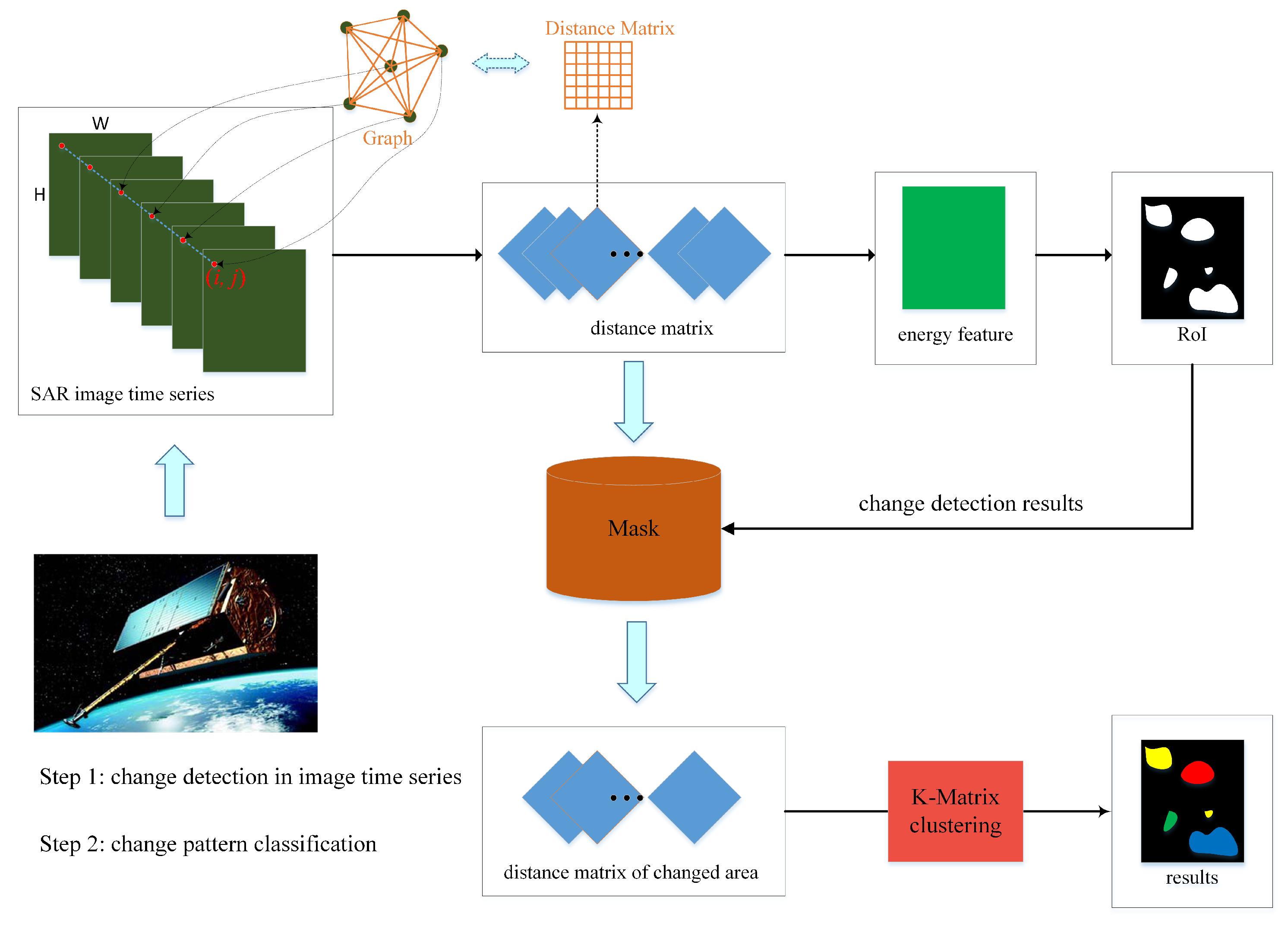
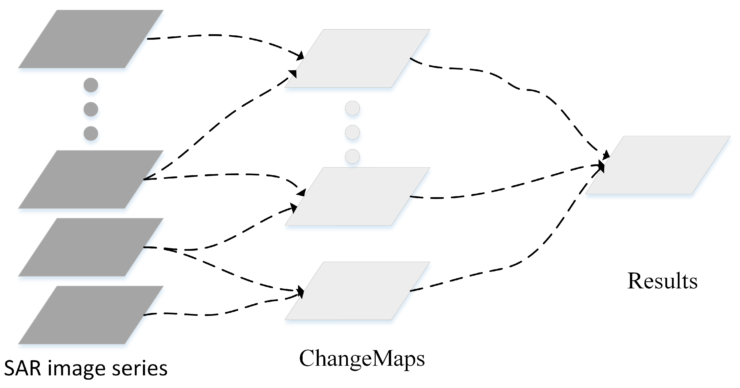
Figure 1 shows the scheme of the proposed method that consists of two main steps: (1) change detection in SAR image time series; (2) change-pattern clustering. First, the detected region of interest (RoI) separates changed from unchanged pixels in SAR image time series. Afterward, the method focuses on the changed pixels only. A novel clustering algorithm is used to mine different change patterns on the RoI in SAR image time series. Finally, the different kinds of change patterns are grouped and visualized by analyzing clustering results.
2.1. Change Detection in SAR Image Time Series
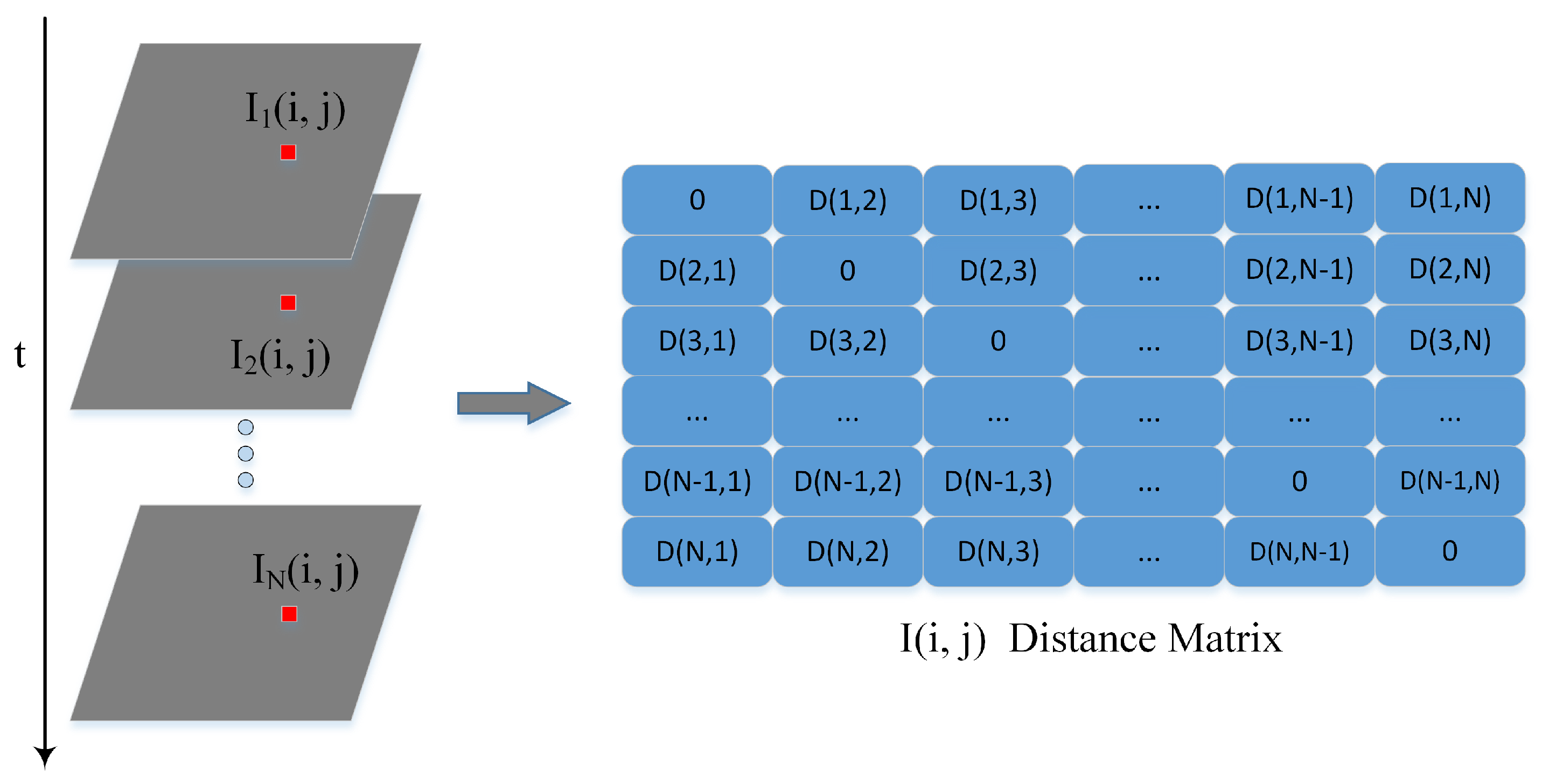
To detect the pixels that have been changed in SAR image time series, we construct a distance matrix containing of the information on responses of distance between each pair of pixels from different dates. Considering an N-length co-registered SAR image time series , where is the SAR image acquired at time t. At the position , we obtain a pixel set , named pixel time series, and represents the amplitude value of SAR image located in . As shown in Figure 2, the distance matrix is computed by:
where the dissimilarity is computed between each two dates using small sliding window to suppress the influence of noise in SAR images. For example, the dissimilarity measurement can be obtained by the Log-Ratio (LR) operator or other measure that can be used in SAR images. This matrix contains all information of dissimilarity which is relevant to the degree of change corresponding to each reference date.
After that, our purpose is to analyze each pixel time series using the corresponding distance matrix. For a pixel time series, we assume that these pixels form a physical system. In physics, it is well known that the lower the energy the more stable for a system. Here, we define similarly the stability of the pixel system, i.e., it is stable if there is no change in terms of feature value of pixels while the degree of instability is corresponding to the changing degree of the pixel. Moreover, the distance matrix records the dissimilarity between any two pixels in time series, so that we redefine the energy value of the pixel system just like the definition of energy in gray-level co-occurrence matrix (GLCM):
Theoretically, only when , the system is completely stable. However, in fact, even after radiation correction, the amplitude value of the pixels in SAR image time series still have some fluctuations. To decide whether there is the stable pixel system or not, the value of energy e is compared to a threshold . The stability information, i.e., change information, is then defined as:
where R is a binary matrix mask with the size of containing 0 and 1 values, in which 0 represents “unchanged” and 1 represents “changed”. In this paper, we consider the changed region as region of interest (RoI), where this region is the main study area in our change-pattern mining experiments.
2.2. K-Matrix Clustering Algorithm
In this section, we propose a novel centroid-based clustering algorithm, called K-Matrix that can preserve the feature shapes of time series using distance matrix. Specifically, we first present our distance measure, called the matrix cross-correlation, which is inspired by the cross-correlation measure for time-lagged signal in [32]. Based on this distance measure, we propose a method to compute the barycenter, i.e., the centroid of matrix clusters. Finally, we describe our K-Matrix clustering algorithm, which relies on an iterative refinement procedure.
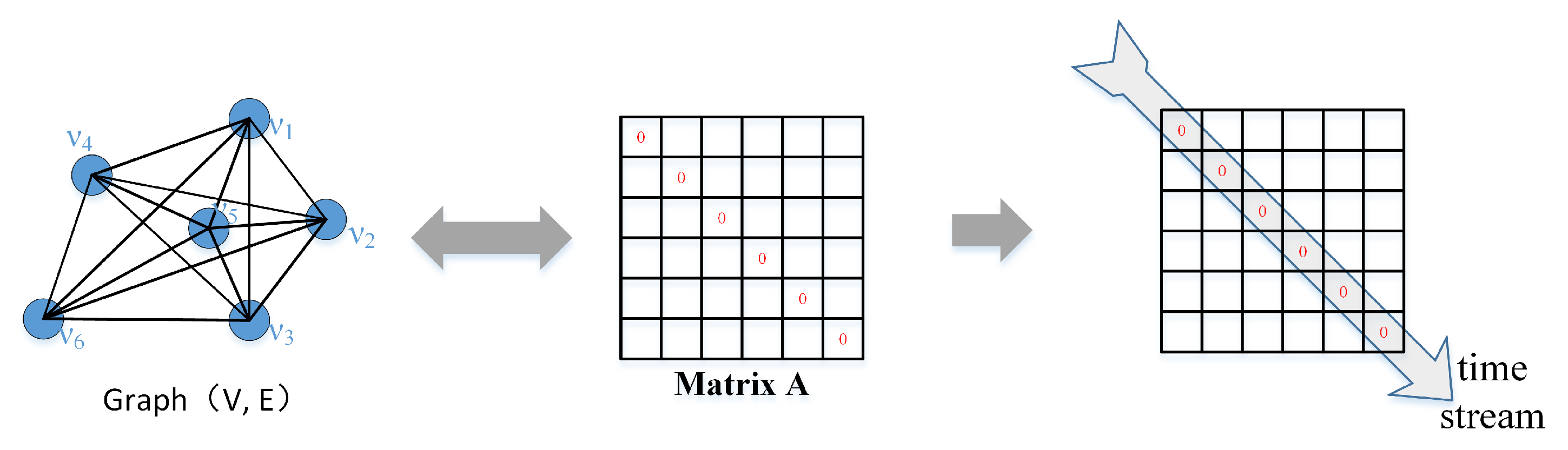
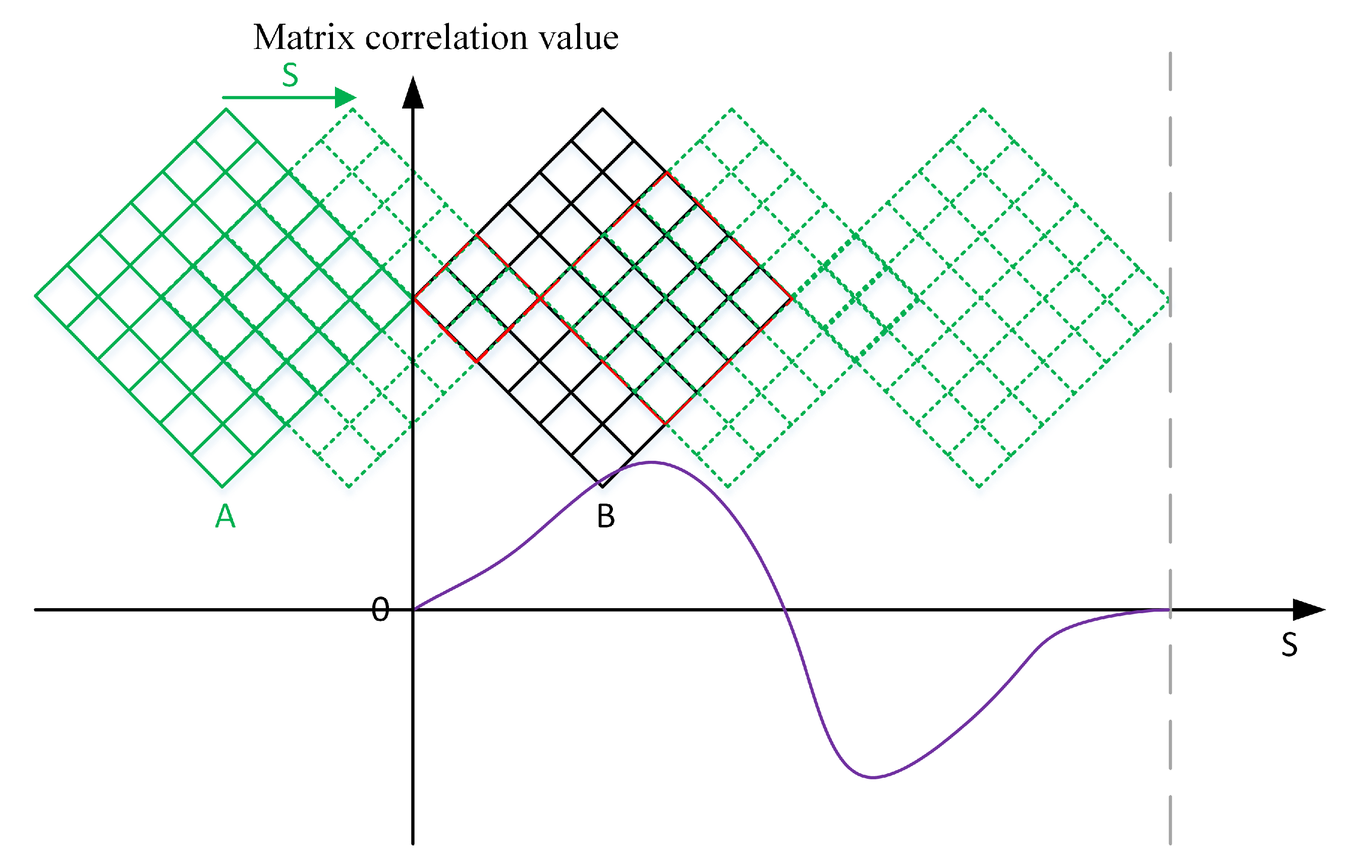
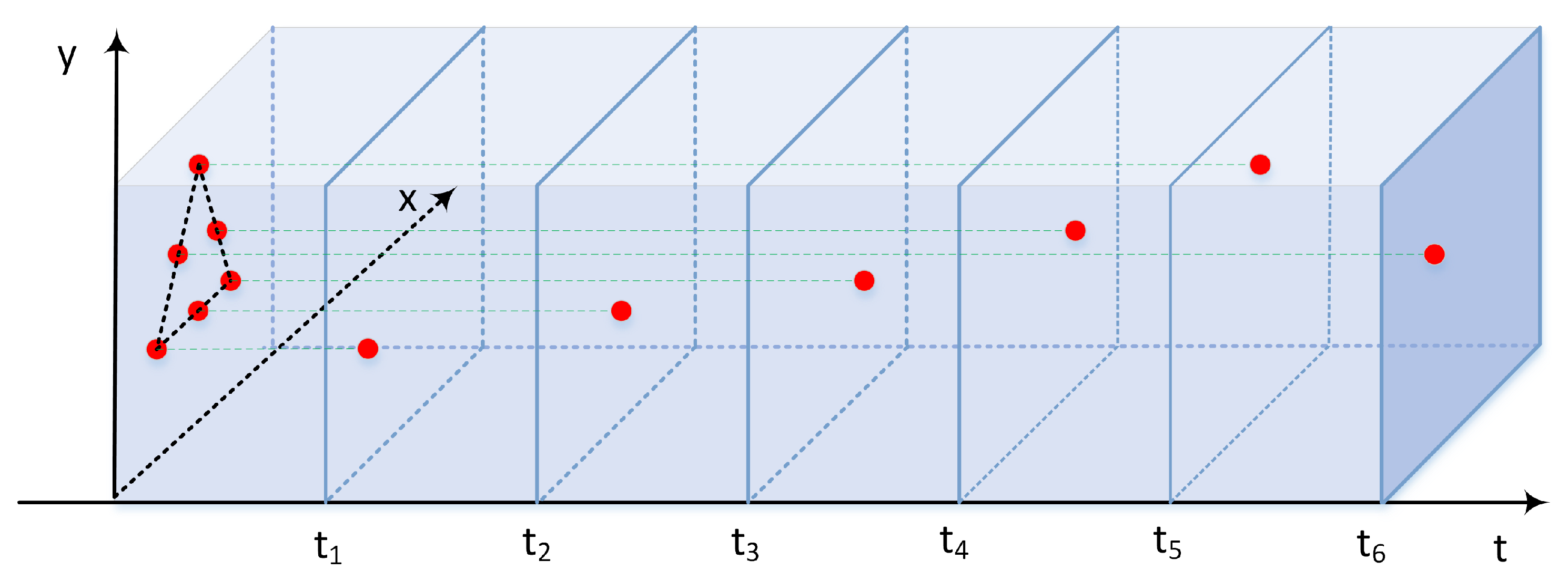
Originally, cross-correlation is a statistical measure with which we can determine the similarity of two time series. Here, this measurement is used to measure the similarity between two distance matrices. For each distance matrix, there is a corresponding graph in the feature space. As shown in Figure 3, in the graph , the vertex represents the feature point extracted from . We define the pixel time series at the spatial position as a pixel system and define the corresponding Graph in its feature space, i.e., vertex represents the feature of the pixel in the feature space and the distance between features of pixel and pixel is defined as edge . All elements of their distance matrix are set to 0 for the diagonal and the time flow information is hidden in the diagonal direction as shown in Figure 3. Considering two distance matrices, A and B, to achieve shift-invariance, we keep B static and slide diagonally A over B to compute their inner product for each shift matrix of A. We denote the time shift of a matrix by a shift variable s:
When all possible shifts are considered, with , there is a matrix cross-correlation sequence (MCC), with length , defined as follows:
Then, we need to determine the position q at which is maximized. In addition, based on this value of q, we can find the optimal time shift of matrix A corresponding to the matrix B. The computational procedure of the matrix cross-correlation sequences is illustrated in Figure 4. Specifically, we define the maximum of the matrix cross-correlation as the similarity between two distance matrices, named matrix cross-correlation similarity ():
For many clustering tasks, it is a challenging step to extract the meaningful centroid according to the proposed distance measurement. Although there are many clustering criteria that have been proposed to capture homogeneity and separation [33], the minimum within-class sum of squared distances is the most commonly used. For example, there is a set including n samples , where , then the goal is to group X into k clusters , and the objective loss function is:
However, if we replace the distance with the similarity measurement, the above formulas can be rewritten as:
In this task of distance matrix clustering, assuming that there is a matrix set in which all elements belong to the same group , where n is the number of elements in , and is one of the cluster center set P. Now we have:
It is difficult to solve this optimization problem directly because it is nonlinear. As mentioned earlier, we can obtain the aligned matrix when the matrix cross-correlation is the maximum. So that we can use these aligned matrix set to substitute . For simplicity, we will express this equation with vector. The distance matrix is symmetrical matrix and it can be written as:
where U and L are an upper triangular matrix and a lower triangular matrix, respectively. Here, the non-zero elements of the matrix U are sequentially taken to compose a vector . Similarly, vector is corresponding to the center matrix . Then Equation (9) is rewritten as (please see Appendix A for more details):
Now, this problem has been converted to a well-known problem named maximization of Rayleigh Quotient [34]. The solution is the eigenvector corresponding to the largest eigenvalue of matrix M. After that, we can restore the center matrix by vector .
It should be noted that the K-Matrix clustering algorithm is based on the iterative refinement procedure just like the one used in K-means. At first, we choose randomly K matrices as centroid to initialize the algorithm. Then, in every iteration, K-Matrix includes two steps: assignment and refinement. In the assignment step, we update the cluster memberships by assigning each matrix to the closest cluster (Equation (6)). In the refinement step, we use the cluster memberships assigned in previous step to update the centroid (Equation (A3)). This algorithm repeats above two steps until the assignment is unchanged or the default maximum number of iterations is reached.
3. Experiment
3.1. Description of Datasets
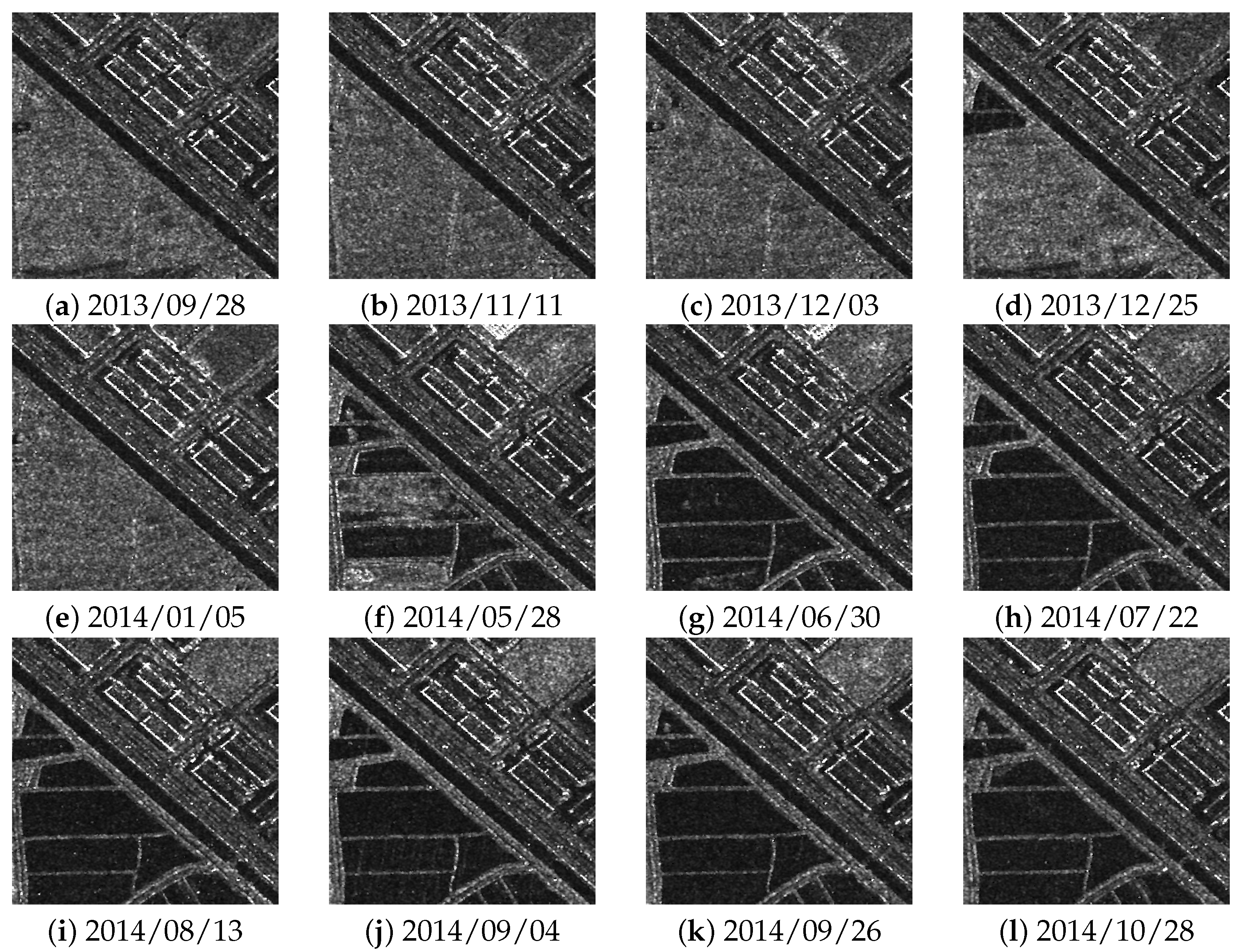
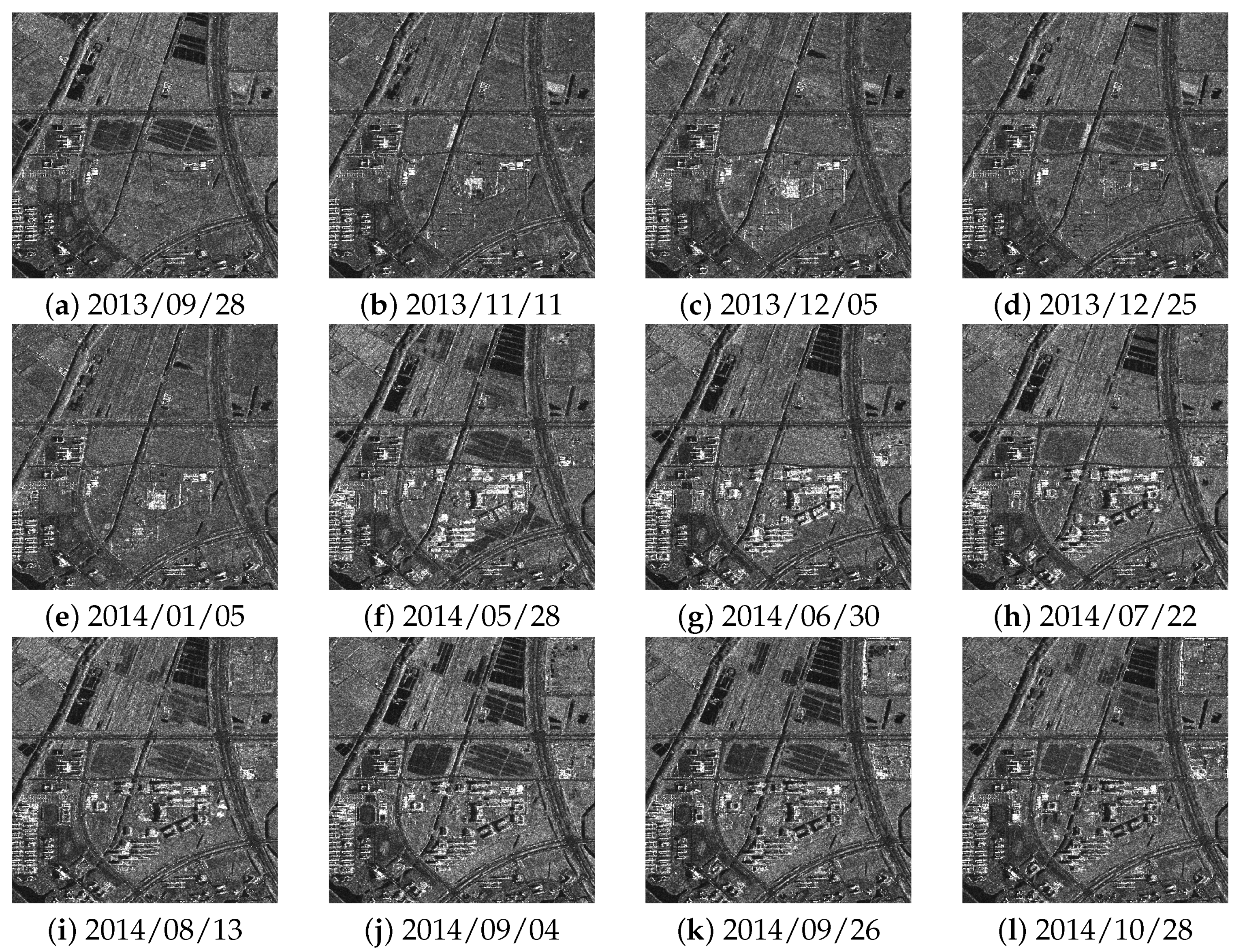
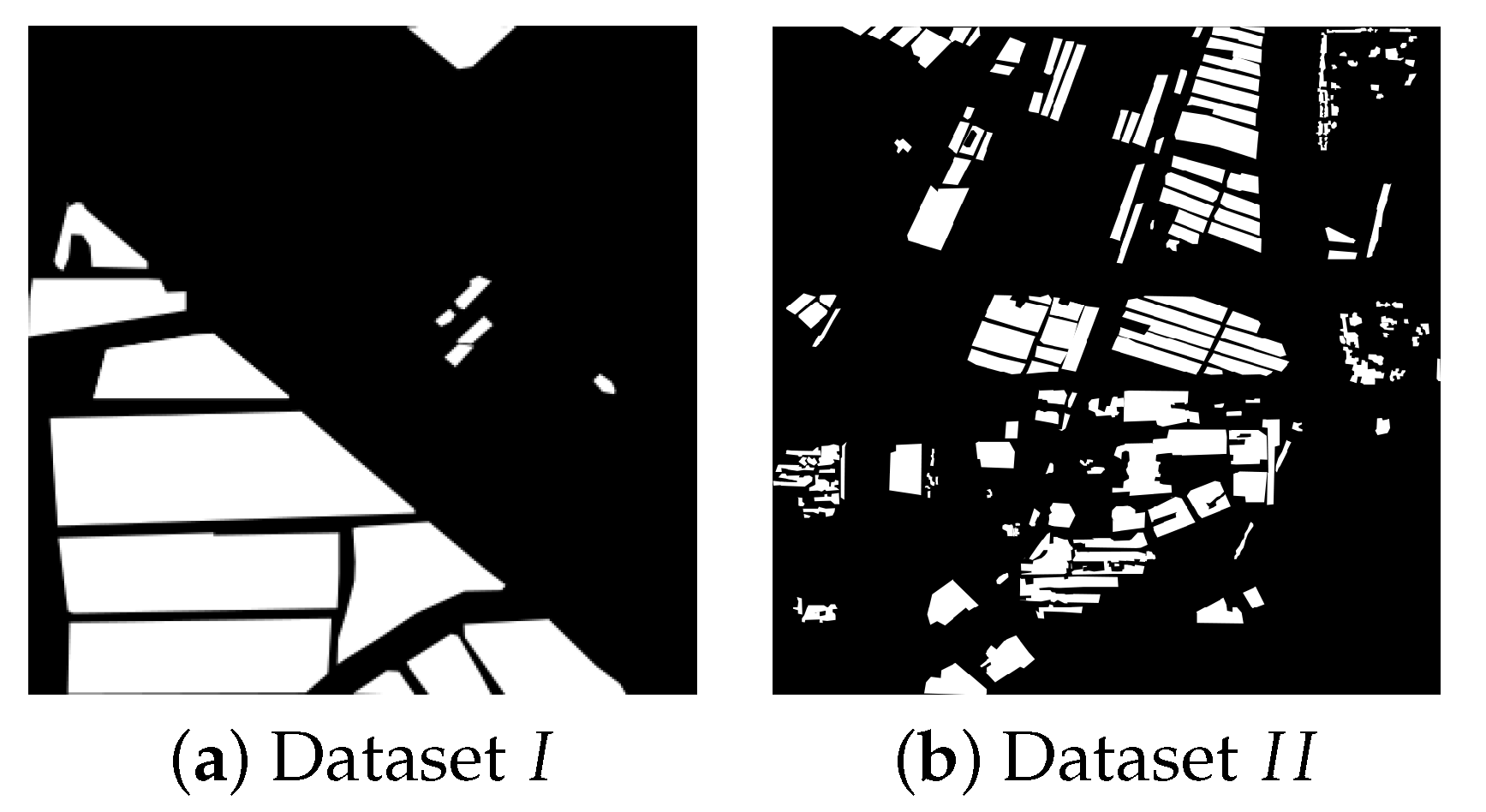
There are two real datasets of SAR image time series used to test the proposed method. These images are acquired with TerraSAR-X sensor over Shanghai, China. The product type is single look complex (SLC) and the imaging mode is StripMap (SM). Both dataset I and dataset contain the co-registered 12 SAR images. They have the same spatial resolution of 3 m × 3 m. The size of each image in dataset I is pixels and the size of each image in dataset is pixels. These SAR images are obtained from 28 September 2013 to 18 October 2014. There are more details shown in Figure 5 and Figure 6. All SAR images have been denoised by MuLoG + BM3D before change detection and pattern mining [16]. The two ground truth maps of change detection are shown in Figure 7, i.e., as long as the change occurs in pixel time series, the corresponding spatial position is set to 1.
3.2. Change Detection in SAR Image Time Series
In this section, our goal is to find the area where the change has occurred. At first, the distance matrix set must be constructed effectively. In this experiment, Log-Ratio (LR) operator and GLRT are selected as the dissimilarity measurements to compute the distance between two pixels for simplicity. Those distance measures based on statistical distribution usually have high computational complexity, such as KL divergence. Moreover, a sliding window is used to suppress the influence of noise when the distance is calculated. Here, the size of the sliding window is set as . The Log-Ratio operator is defined as follows:
where is the mean operator, indexes the spatial position of the pixel in the image. According to [35], the similarity of the generalized likelihood ratio is written as:
where is the pixel in patch and is the (equivalent) number of looks of . Then, the distance can be denoted as:
The distance matrix is obtained after computing distance of all pixel pairs. In this way, we have the distance matrix set . Here, we chose a commonly used time series change detection framework for comparison [36]. As shown in Figure 8, the results are obtained by summing the ChangeMaps of all adjacent two dates.
For our change detection experiments, we use the following four indicators to evaluate these methods: Overall Accuracy (OA), the detection precision of changed pixels (Pc), the recall of changed pixels (Rc) and Kappa coefficient. They are defined as follows:
where TP means the number of true detected changed pixels, TN means the number of true detected no changed pixels, FP means the number of false detected changed pixels and FN means the number of false detected no changed pixels. Moreover, is defined as:
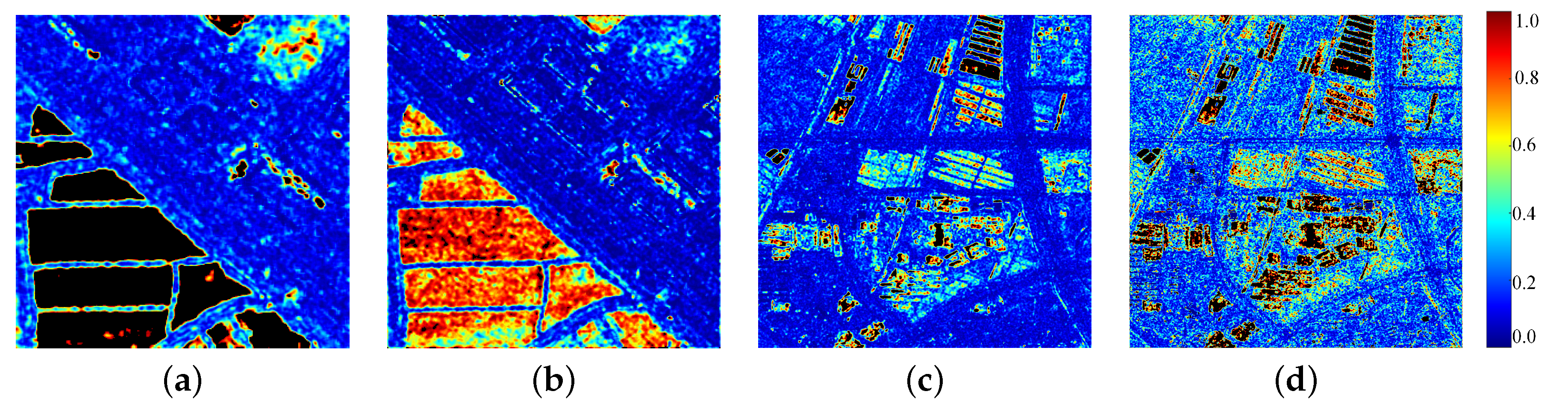
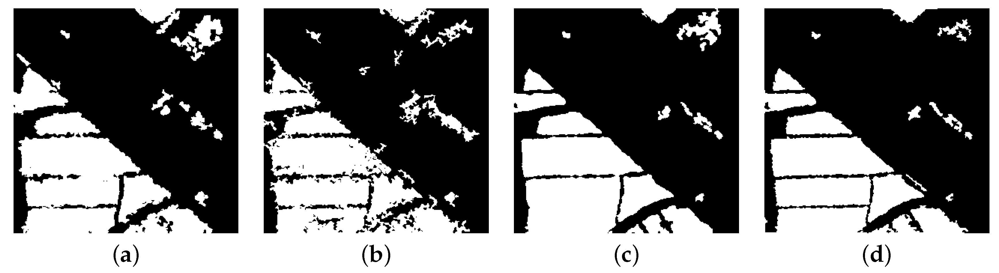
For the dataset I, the value of N is 12. The values of m and n both are 300. According to the Formula (2), the energy value e can be computed and the feature maps are shown in Figure 9a,b. The feature map can are considered to be the activity map that the greater the value, the bigger the change. As shown in Figure 9, the Log-Ratio operator is sensitive to the change of the water area. Furthermore, to determine the changed area, i.e., region of interest (RoI), the thresholding algorithm is used to generate the binary map that the zeros represent the unchanged pixels and the ones represent the changed pixels. Here, the GKI algorithm is applied to separate the changed pixels from the unchanged pixels. The change detection results are shown in Figure 10. In Table 1, the performance of the proposed method is clearly better than the traditional one. The GLRT method has the highest overall accuracy (OA = 96.27%), detection precision of changed pixels (Pc = 91.94%), recall (Rc = 95.03%) and the best classification result (Kappa = 0.91).
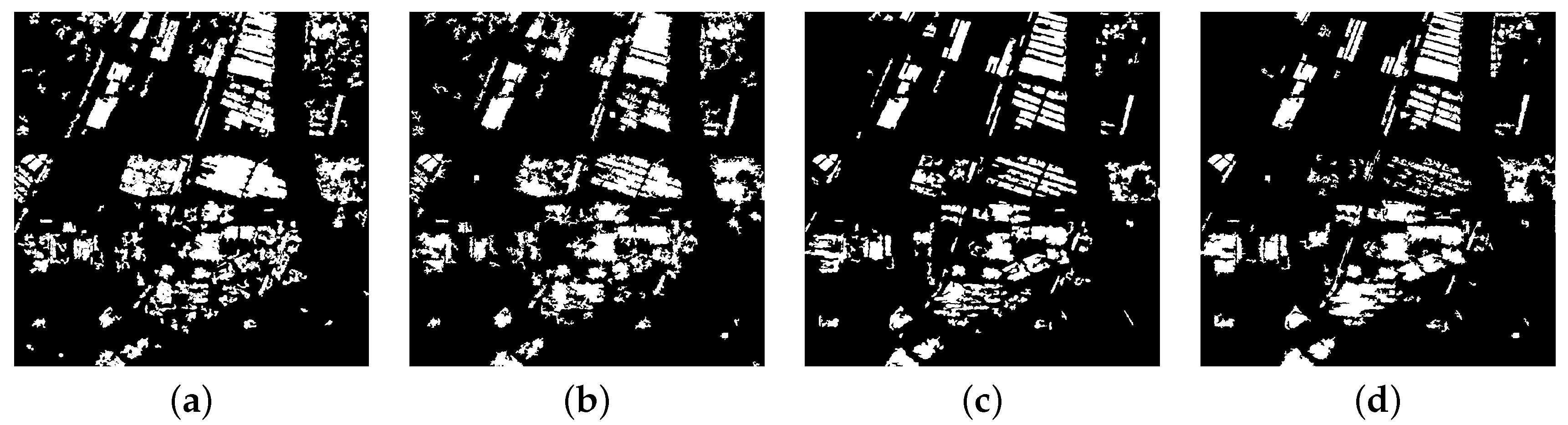
For the dataset , the value of N is 12. The values of m and n both are 800. The distance matrix set is obtained by calculating the each distance matrix at the spatial position . Based the LR operator and GLRT, the distance matrix sets are obtained. Then, the feature maps are computed and shown in Figure 9c,d. Figure 11 shows the change detection results obtained by using the GKI algorithm. It is obvious that the LR operator method and GLRT method in our scheme have better performance of change detection. The quantitative analysis results are listed in Table 2. Please note that all the evaluation indicators of change detection are lower than these in dataset I because there are more complex scene in the dataset . However, our scheme with GLRT method still has the satisfactory performance with Pc 75.89%, Rc 73.78%, OA 92.84% and Kappa 0.70.
3.3. Change-Pattern Mining
After detecting changes in SAR image time series, our next goal is to discover these different change patterns. In Section 3.2, the distance matrix set has been obtained and results with the best performance are defined as change map. In this section, the above change detection results are considered to be the study area. The change map is an m-by-n matrix containing only 0 and 1. Then, we denote a new distance matrix set :
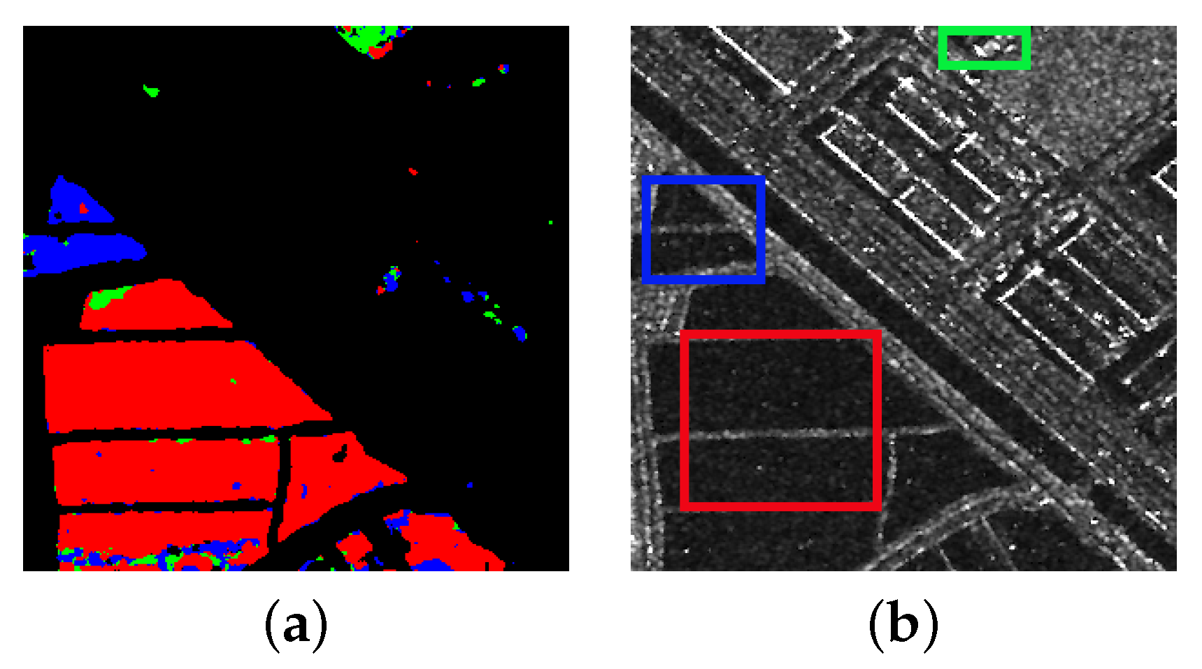
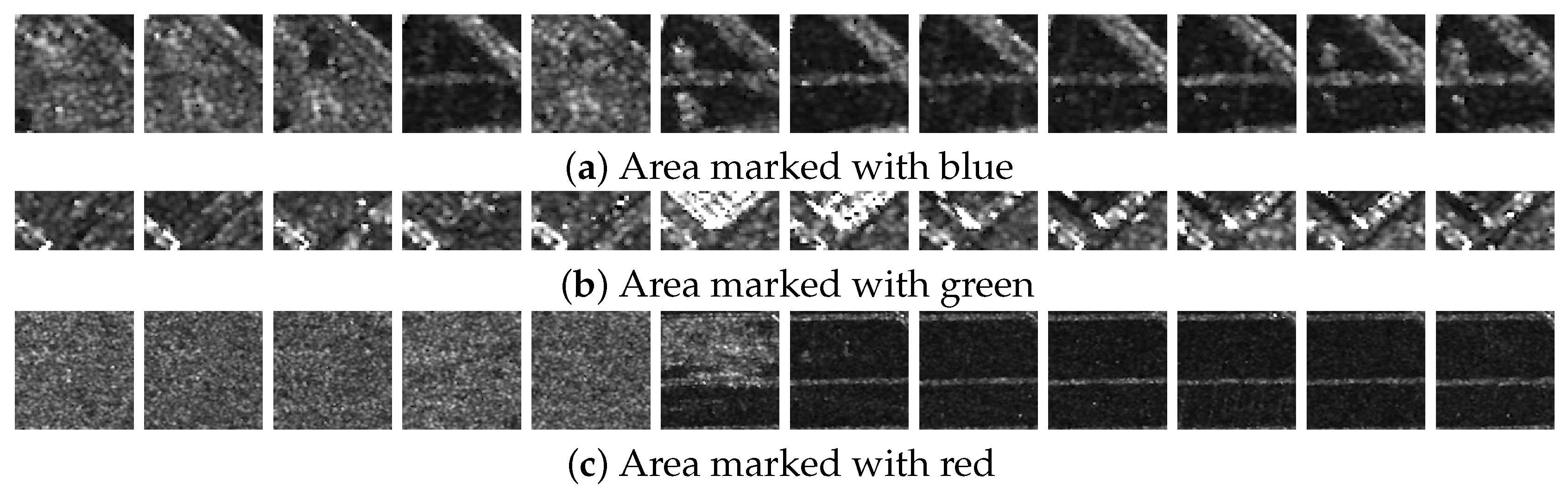
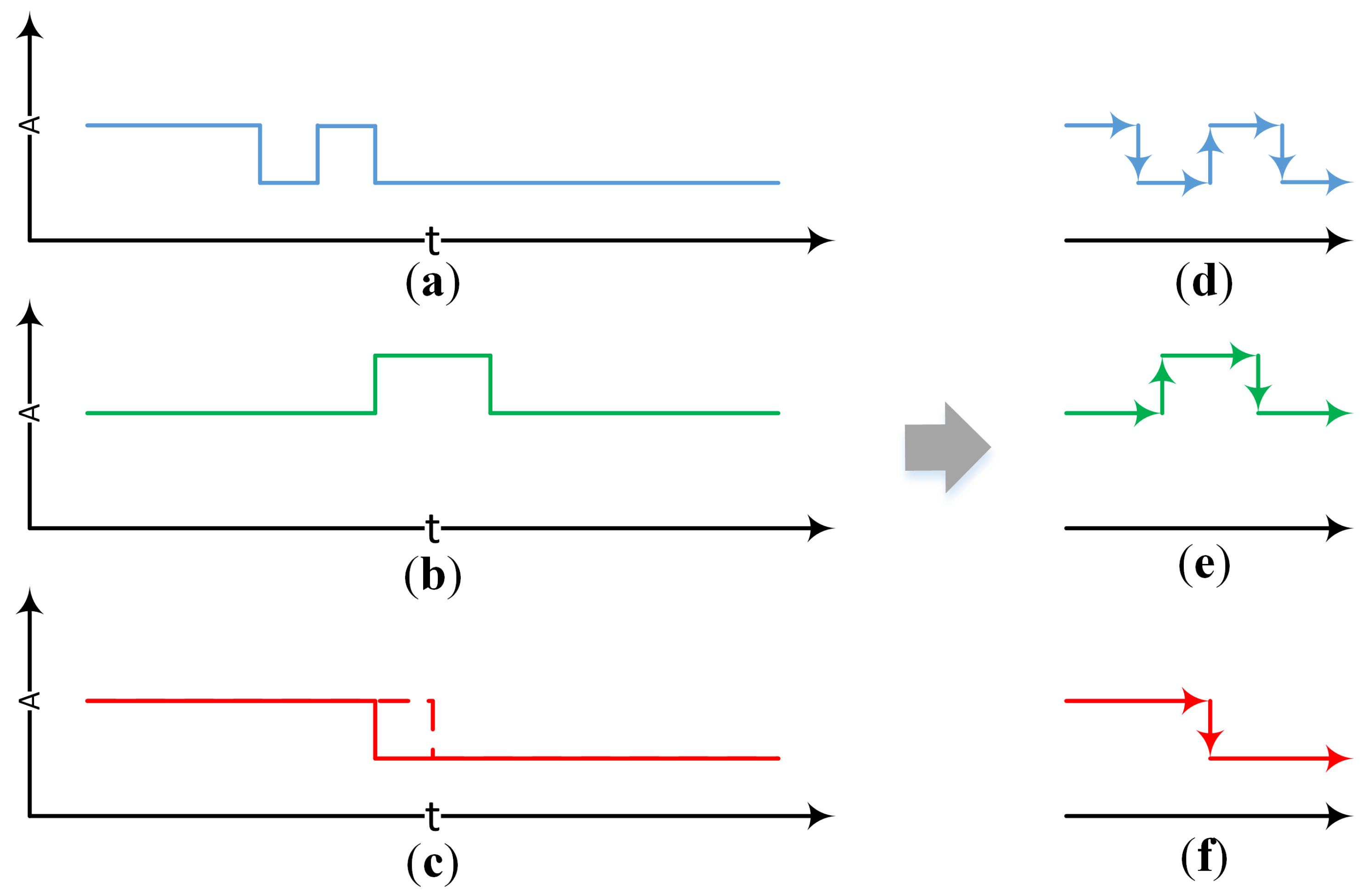
Each element in is a distance matrix of the changed pixel. We apply the proposed K-Matrix clustering algorithm to two time series datasets. In this experiment, we only use the amplitude information of SAR images. For dataset I, we randomly choose three distance matrices to initialize K-Matrix algorithm from a practical point of view. The clustering results of change patterns are shown in Figure 12. Three areas with different change patterns are marked in red, green, and blue, respectively. In Figure 12b, three typical change-pattern areas are marked with three different color rectangles. We crop these areas and show them in Figure 13. It is obvious that the area marked with green represents the change of buildings (Figure 13b). Figure 13a,c both represent the change in the water areas, but they belong to different change patterns. Figure 14 shows a better visualization. Figure 14a–c represent three different changes of the amplitude along time and the corresponding change patterns are shown in Figure 14d–f. Remarkably, the solid line and the dotted line in Figure 14c represent two kinds of changes corresponding to Figure 13c, where the two-step changes occur in different time but they both belong to the same change pattern shown in Figure 14f.
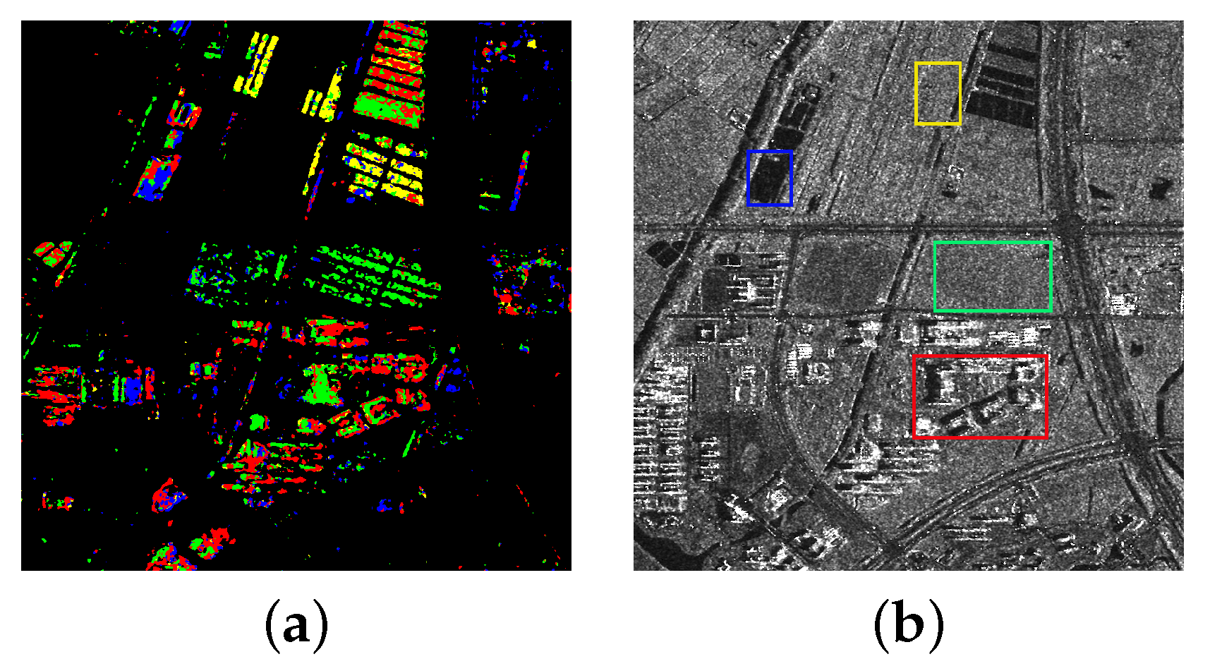
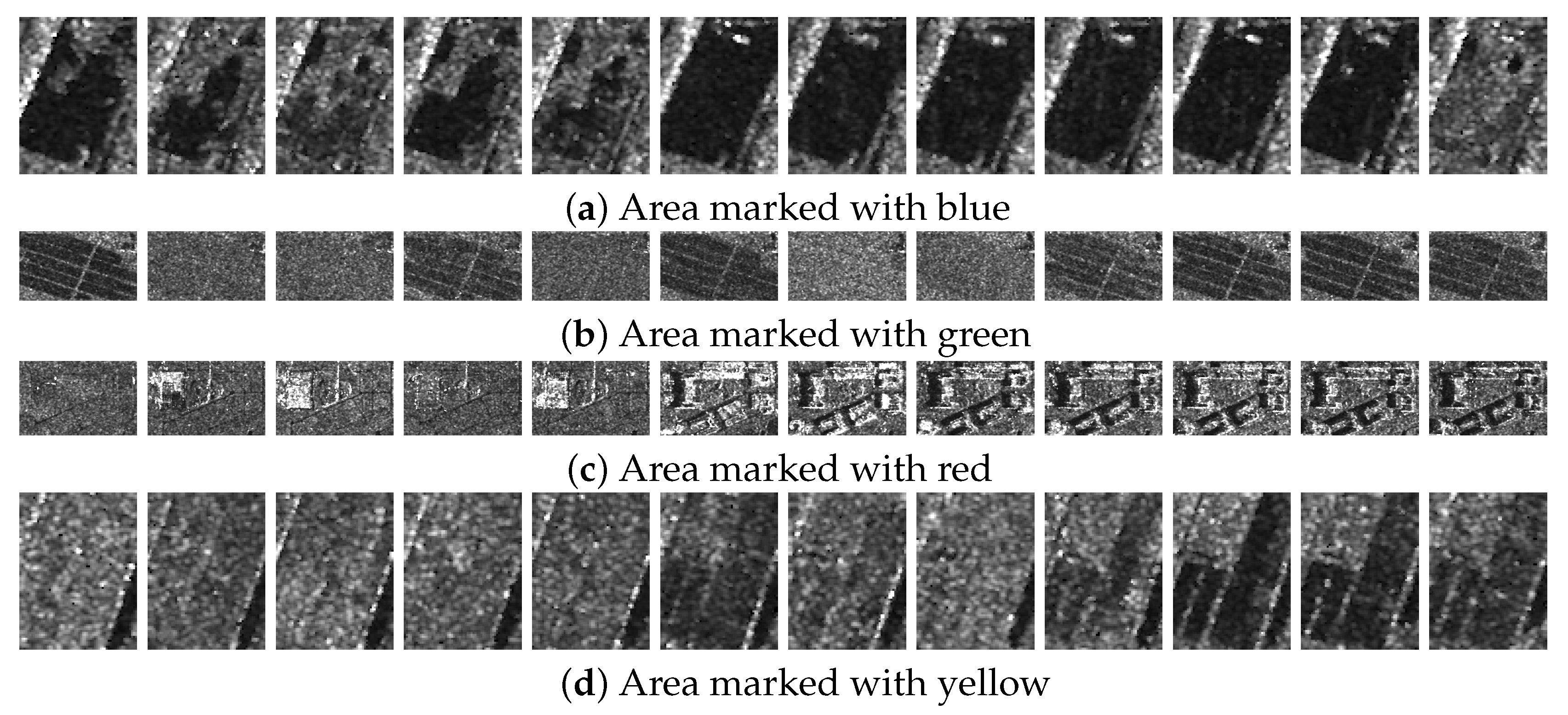
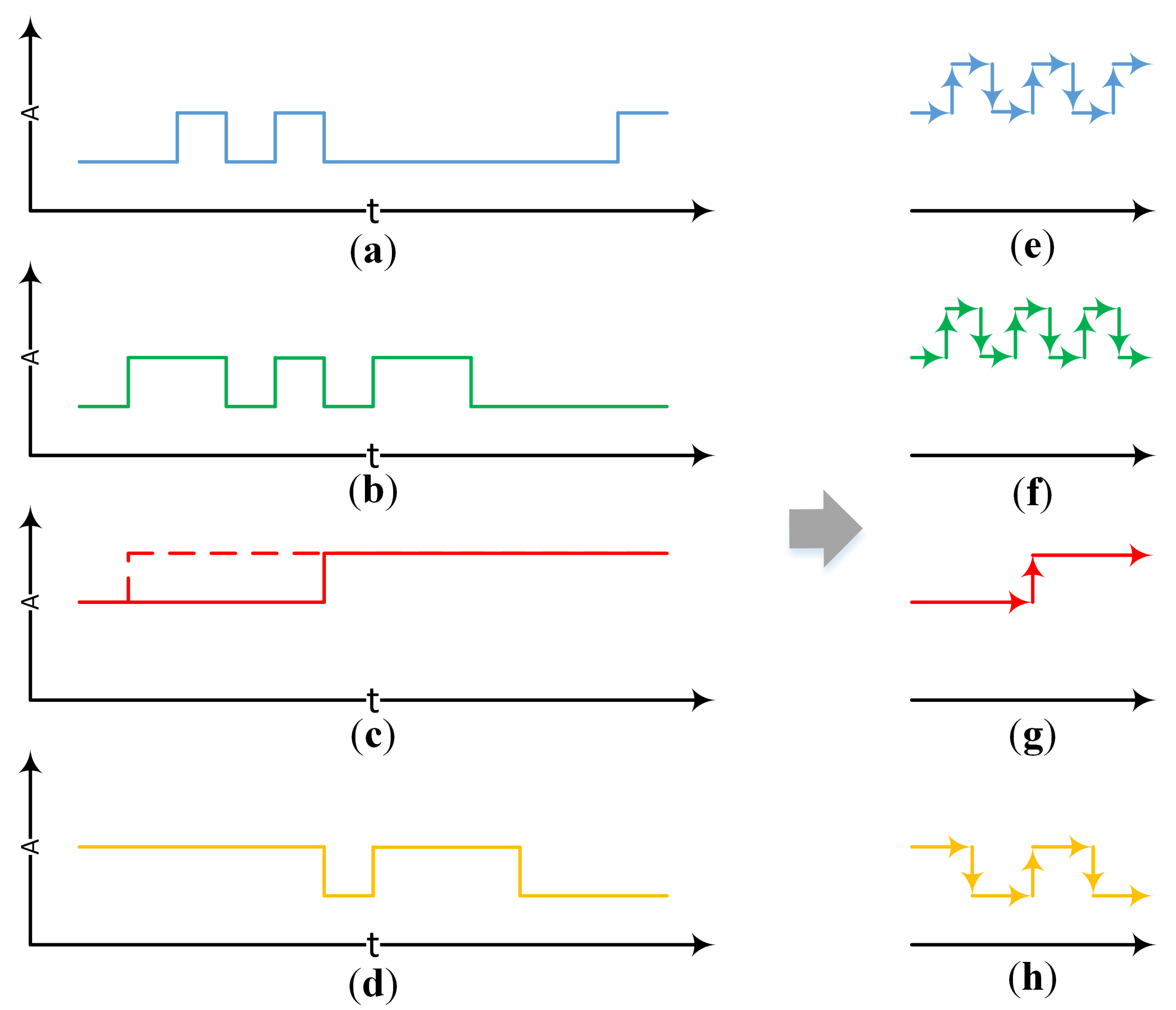
For dataset , these SAR images have larger sizes and more complex change patterns. The clustering algorithm starts with the number of patterns being set to 4. The clustering results shown in Figure 15a are painted in four colors: red, green, blue, and yellow. In Figure 16c, the area marked by red rectangle is mainly the change of buildings. Due to the overlap and multiple scattering of high buildings, the clustering results have multiple change patterns mixed together. In Figure 16b, the area marked by green rectangle is likely to be a periodic wetland change pattern. The regions marked by blue and yellow rectangles represent two water areas with different change periods such as the areas shown in Figure 16a,d. More results are displayed in Figure 17. Figure 17a–d indicate four different fluctuations and their corresponding change patterns are extracted in Figure 17e–h. For example, the red solid line and dotted line both belong to the change patterns of buildings since they are constructed in different dates.
4. Discussion
Change detection and change-pattern analysis of SAR image time series play a great role in Earth monitoring. It is a huge challenge to handle large amounts of remote sensing data while the area that changes is usually only a small part. The proposed change detection method is only used to detect whether a time series has changed and cannot detect where the change occurred. For a distance matrix, if the pixels of corresponding time series have not changed, the value of each element in the distance matrix is very small. if the pixel in the ith position changes, the values of the elements of the ith row and the ith column are larger than the values of other elements. Each time series with a different change pattern has a distance matrix corresponding to it.
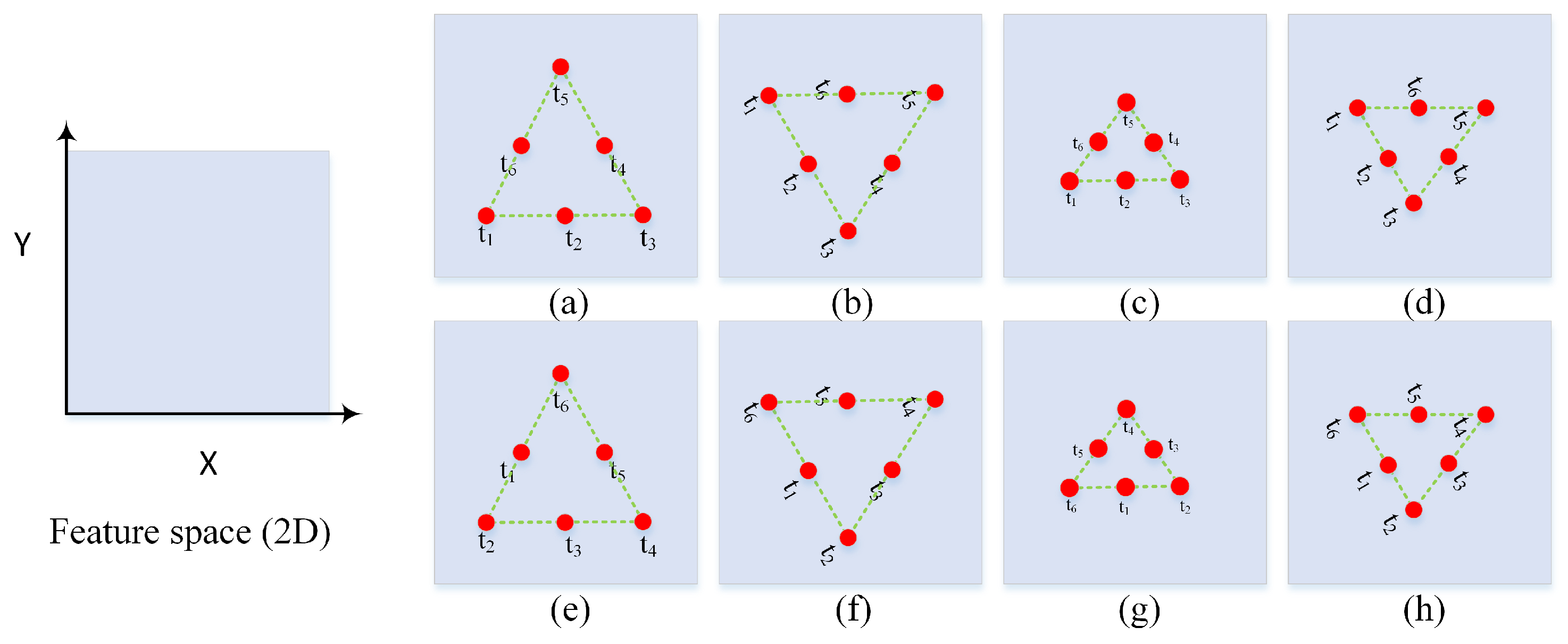
To discover change patterns from the changed area, we propose a clustering algorithm based on distance matrices, called K-Matrix. Inspired by cross-correlation, the matrix cross-correlation is defined, and we expect that this method can cluster pixels with the same change trend into a group. As shown in Figure 14c and Figure 17c, the solid line and dotted line are grouped the same cluster. In our experiment, only the amplitude characteristics of the pixels are used. From a theoretical point of view, the K-Matrix can be used to cluster the change patterns in multidimensional feature space. Figure 18 and Figure 19 show the possible results of this method in 2-dimensional feature space of pixel time series. However, when we use multidimensional features, the final clustering results are difficult to visualize and whether the discovered patterns have obvious physical meaning is not clear. As an exploration in change-pattern mining of SAR time series, although our method achieves desirable results on two real datasets, there still exist certain limitations. For example, because the two-step scheme relies on the distance matrix, how to compute the distance between two pixels effectively is a problem worth thinking about. Moreover, the numerical complexity of distance matrix construction and the K-Matrix algorithm are and , respectively, where m and n are the sizes of SAR images, N is the number of images. With the length of SAR image time series increasing, the computation cost and storage space of distance matrices will be very high. In the future, we will study the correspondence between the distance matrices of changed pixels and different change patterns and some more efficient algorithms to discover patterns with special physical meanings will be investigated.
5. Conclusions
In this paper, a new framework for the change-pattern mining of SAR image time series has been proposed. The method is based on the distance matrix which records the dissimilarity of two pixels at the same spatial position in time series. A novel method is proposed to detect the changes in the SAR image time series. The proposed K-Matrix is used to cluster the distance matrix into different groups. Based on our framework, the Log-Ratio operator and GLRT are used in change detection of SAR image time series. The accuracy and Kappa are used to evaluate the performance of the proposed method. Finally, we use the proposed K-Matrix to discover the change patterns based on the change detection results. Experimental results on two datasets of TerraSAR-X image time series illustrate the effectiveness of the proposed method.
Author Contributions
D.P. and W.Y. provided the original idea for the study, supervised the research and contributed to the article’s organization. T.P. and H.-C.L. contributed to the discussion of the design. D.P. drafted the manuscript, which was revised by all authors. All authors read and approved the final manuscript.
Funding
The research was partially supported by the National Natural Science Foundation of China (NSFC) under Grant 61771351 and Grant 61871335, the CETC key laboratory of aerospace information applications under Grant SXX18629T022, and the project for innovative research groups of the natural science foundation of Hubei Province (No. 2018CFA006).
Acknowledgments
Sincere thanks are given to the anonymous reviewers and members of the editorial team for their comments and valuable contributions.
Conflicts of Interest
The authors declare no conflict of interest.
Appendix A
Here, Equation (9) is rewritten as:
Considering the high time complexity of sum operation, we convert it into a matrix multiplication:
where . Moreover, we set to obtain the z-normalized , where I is the identify matrix, and O is a matrix with all ones [32]. Finally, by dividing to make unit norm, we obtain:
where .
References
- Lu, D.; Mausel, P.; Moran, E.F. Change detection techniques. Int. J. Remote Sens. 2004, 25, 2365–2407. [Google Scholar] [CrossRef]
- Quegan, S.; Toan, T.L.; Yu, J.J.; Ribbes, F.; Floury, N. Multitemporal ERS SAR analysis applied to forest mapping. IEEE Trans. Geosci. Remote Sens. 2000, 38, 741–753. [Google Scholar] [CrossRef]
- Muro, J.; Canty, M.J.; Conradsen, K.; Huttich, C.; Nielsen, A.A.; Skriver, H.; Remy, F.; Strauch, A.; Thonfeld, F.; Menz, G. Short-Term Change Detection in Wetlands Using Sentinel-1 Time Series. Remote Sens. 2016, 8, 795. [Google Scholar] [CrossRef]
- Chen, F.; Lasaponara, R.; Masini, N. An overview of satellite synthetic aperture radar remote sensing in archaeology: From site detection to monitring. J. Cult. Herit. 2017, 23, 5–11. [Google Scholar] [CrossRef]
- Brunner, D.; Bruzzone, L.; Lemoine, G. Change detection for earthquake damage assessment in built-up areas using very high resolution optical and SAR imagery. IEEE Int. Geosci. Remote Sens. Symp. 2010, 1, 3210–3213. [Google Scholar]
- Bovolo, F.; Bruzzone, L. A Split-Based Approach to Unsupervised Change Detection in Large-Size Multitemporal Images: Application to Tsunami-Damage Assessment. IEEE Trans. Geosci. Remote Sens. 2007, 45, 1658–1670. [Google Scholar] [CrossRef]
- Gamba, P.; Dellacqua, F.; Lisini, G. Change Detection of Multitemporal SAR Data in Urban Areas Combining Feature-Based and Pixel-Based Techniques. IEEE Trans. Geosci. Remote Sens. 2006, 44, 2820–2827. [Google Scholar] [CrossRef]
- Heine, I.; Jagdhuber, T.; Itzerott, S. Classification and Monitoring of Reed Belts Using Dual-Polarimetric TerraSAR-X Time Series. Remote Sens. 2016, 8, 552. [Google Scholar] [CrossRef]
- Brown, W.M. Synthetic Aperture Radar. IEEE Trans. Aerosp. Electron. Syst. 1967, 2, 217–229. [Google Scholar] [CrossRef]
- Yang, W.; Zhong, N.; Yan, T.; Yang, X. Classification of Polarimetric SAR Images Based on the Riemannian Manifold. J. Radars 2017, 6, 43-3-441. [Google Scholar]
- Bruzzone, L.; Bovolo, F. A Novel Framework for the Design of Change-Detection Systems for Very-High-Resolution Remote Sensing Images. Proc. IEEE 2013, 101, 609–630. [Google Scholar] [CrossRef]
- Gao, F.; Liu, X.; Dong, J.; Zhong, G.; Jian, M. Change Detection in SAR Images Based on Deep Semi-NMF and SVD Networks. Remote Sens. 2017, 9, 435. [Google Scholar] [CrossRef]
- Hu, H.; Ban, Y. Unsupervised Change Detection in Multitemporal SAR Images Over Large Urban Areas. IEEE J. Sel. Top. Appl. Earth Obs. Remote Sens. 2014, 7, 3248–3261. [Google Scholar] [CrossRef]
- Argenti, F.; Lapini, A.; Bianchi, T.; Alparone, L. A Tutorial on Speckle Reduction in Synthetic Aperture Radar Images. IEEE Geosci. Remote Sens. Mag. 2013, 1, 6–35. [Google Scholar] [CrossRef] [Green Version]
- Deledalle, C.; Denis, L.; Poggi, G.; Tupin, F.; Verdoliva, L. Exploiting Patch Similarity for SAR Image Processing: The nonlocal paradigm. IEEE Signal Process. Mag. 2014, 31, 69–78. [Google Scholar] [CrossRef]
- Deledalle, C.; Denis, L.; Tabti, S.; Tupin, F. MuLoG, or How to Apply Gaussian Denoisers to Multi-Channel SAR Speckle Reduction? IEEE Trans. Image Process. 2017, 26, 4389–4403. [Google Scholar] [CrossRef] [Green Version]
- Singh, A. Digital change detection techniques using remotely sensed data. Int. J. Remote Sens. 1989, 10, 989–1003. [Google Scholar] [CrossRef]
- Rignot, E.; Van Zyl, J.J. Change detection techniques for ERS-1 SAR data. IEEE Trans. Geosci. Remote Sens. 1993, 31, 896–906. [Google Scholar] [CrossRef] [Green Version]
- Lombardo, P.; Oliver, C.J. Maximum likelihood approach to the detection of changes between multitemporal SAR images. IEE Proc.-Radar Sonar Navig. 2001, 148, 200–210. [Google Scholar] [CrossRef]
- Inglada, J.; Mercier, G. A New Statistical Similarity Measure for Change Detection in Multitemporal SAR Images and Its Extension to Multiscale Change Analysis. IEEE Trans. Geosci. Remote Sens. 2011, 45, 1432–1445. [Google Scholar] [CrossRef]
- Yang, W.; Song, H.; Huang, X.; Xu, X.; Liao, M. Change Detection in High-Resolution SAR Images Based on Jensen–Shannon Divergence and Hierarchical Markov Model. IEEE J. Sel. Top. Appl. Earth Obs. Remote Sens. 2014, 7, 3318–3327. [Google Scholar] [CrossRef]
- Ostu, N. A threshold selection method from gray-level histograms. IEEE Trans. Syst. Man Cybern. 1978, 9, 62–66. [Google Scholar]
- Kittler, J.; Illingworth, J. Minimum error thresholding. Pattern Recognit. 1986, 19, 41–47. [Google Scholar] [CrossRef]
- Bazi, Y.; Bruzzone, L.; Melgani, F. An unsupervised approach based on the generalized Gaussian model to automatic change detection in multitemporal SAR images. IEEE Trans. Geosci. Remote Sens. 2005, 43, 874–887. [Google Scholar] [CrossRef] [Green Version]
- Moser, G.; Serpico, S.B. Generalized minimum-error thresholding for unsupervised change detection from SAR amplitude imagery. IEEE Trans. Geosci. Remote Sens. 2006, 44, 2972–2982. [Google Scholar] [CrossRef]
- Schulz, K. Change detection in time series of high resolution SAR satellite images. Proc. SPIE Int. Soc. Opt. Eng. 2012, 8538, 06. [Google Scholar]
- Yuan, J.; Lv, X.; Dou, F.; Yao, J. Change Analysis in Urban Areas Based on Statistical Features and Temporal Clustering Using TerraSAR-X Time-Series Images. Remote Sens. 2019, 11, 926. [Google Scholar] [CrossRef]
- Atto, A.M.; Trouve, E.; Berthoumieu, Y.; Mercier, G. Multidate Divergence Matrices for the Analysis of SAR Image Time Series. IEEE Trans. Geosci. Remote Sens. 2013, 51, 1922–1938. [Google Scholar] [CrossRef]
- Quin, G.; Pinel-Puyssegur, B.; Nicolas, J.; Loreaux, P. MIMOSA: An Automatic Change Detection Method for SAR Time Series. IEEE Trans. Geosci. Remote Sens. 2014, 52, 5349–5363. [Google Scholar] [CrossRef]
- Lê, T.T.; Atto, A.M.; Trouvé, E.; Solikhin, A.; Pinel, V. Change detection matrix for multitemporal filtering and change analysis of SAR and PolSAR image time series. ISPRS J. Photogramm. Remote Sens. 2015, 107, 64–76. [Google Scholar] [CrossRef]
- Su, X.; Deledalle, C.; Tupin, F.; Sun, H. NORCAMA: Change analysis in SAR time series by likelihood ratio change matrix clustering. ISPRS J. Photogramm. Remote Sens. 2015, 101, 247–261. [Google Scholar] [CrossRef] [Green Version]
- Paparrizos, J.; Gravano, L. k-Shape: Efficient and Accurate Clustering of Time Series. Int. Conf. Manag. Data 2015, 45, 1855–1870. [Google Scholar]
- Hansen, P.; Jaumard, B. Cluster analysis and mathematical programming. Math. Program. 1997, 79, 191–215. [Google Scholar] [CrossRef] [Green Version]
- Golub, G.H.; Van, L.; Charles, F. Matrix Computations, 3rd ed.; JHU Press: Baltimore, MD, USA, 1996. [Google Scholar]
- Su, X.; Deledalle, C.A.; Tupin, F.; Sun, H. SAR image change detection by likelihood ratio test in multitemporal time series. In Proceedings of the IGARSS 2013, Melbourne, VIC, Australia, 21–26 July 2013. [Google Scholar]
- Boldt, M.; Schulz, K. Change detection in high resolution SAR images: Amplitude based activity map compared with CoVAmCoh analysis. In Proceedings of the IEEE Geoscience and Remote Sensing Symposium, Munich, Germany, 22–27 July 2012; pp. 3803–3806. [Google Scholar]
Figure 1.
Framework of the proposed method.

Figure 2.
The strategy to build a distance matrix.

Figure 3.
Graph and Distance Matrix.

Figure 4.
The cross-correlation between two matrices.

Figure 5.
Dataset I of SAR image time series.

Figure 6.
Dataset of SAR image series.

Figure 7.
Ground truth for SAR image time series.

Figure 8.
The baseline framework of change detection in SAR image time series.

Figure 9.
Feature map. Dataset I: (a) LR, (b) GLRT. Dataset : (c) LR, (d) GLRT.

Figure 10.
Change map, dataset I. (a) Baseline (LR), (b) Baseline (GLRT), (c) Ours (LR), (d) Ours (GLRT).
Figure 10.
Change map, dataset I. (a) Baseline (LR), (b) Baseline (GLRT), (c) Ours (LR), (d) Ours (GLRT).

Figure 11.
Change map, dataset . (a) Baseline (LR), (b) Baseline (GLRT), (c) Ours (LR), (d) Ours (GLRT).
Figure 11.
Change map, dataset . (a) Baseline (LR), (b) Baseline (GLRT), (c) Ours (LR), (d) Ours (GLRT).

Figure 12.
Clustering results, dataset I. (a) Change-pattern mining results, (b) Three typical change-pattern areas marked with three different color rectangles.
Figure 12.
Clustering results, dataset I. (a) Change-pattern mining results, (b) Three typical change-pattern areas marked with three different color rectangles.

Figure 13.
Three different change patterns.

Figure 14.
Change patterns.

Figure 15.
Clustering results, dataset II. (a) Change-pattern mining results, (b) Four typical change-pattern areas marked with four different color rectangles.
Figure 15.
Clustering results, dataset II. (a) Change-pattern mining results, (b) Four typical change-pattern areas marked with four different color rectangles.

Figure 16.
Four different change patterns.

Figure 17.
Change patterns.

Figure 18.
The 2-dimensional feature in time series.

Figure 19.
The different changes of the same change-pattern. Left: the 2-dimensional feature space. Right: (a)–(h) different changes with different orders and scales.
Figure 19.
The different changes of the same change-pattern. Left: the 2-dimensional feature space. Right: (a)–(h) different changes with different orders and scales.


© 2019 by the authors. Licensee MDPI, Basel, Switzerland. This article is an open access article distributed under the terms and conditions of the Creative Commons Attribution (CC BY) license (http://creativecommons.org/licenses/by/4.0/).
Share and Cite
MDPI and ACS Style
Peng, D.; Pan, T.; Yang, W.; Li, H.-C. K-Matrix: A Novel Change-Pattern Mining Method for SAR Image Time Series. Remote Sens. 2019, 11, 2161. https://0-doi-org.brum.beds.ac.uk/10.3390/rs11182161
AMA Style
Peng D, Pan T, Yang W, Li H-C. K-Matrix: A Novel Change-Pattern Mining Method for SAR Image Time Series. Remote Sensing. 2019; 11(18):2161. https://0-doi-org.brum.beds.ac.uk/10.3390/rs11182161
Chicago/Turabian StylePeng, Dong, Ting Pan, Wen Yang, and Heng-Chao Li. 2019. "K-Matrix: A Novel Change-Pattern Mining Method for SAR Image Time Series" Remote Sensing 11, no. 18: 2161. https://0-doi-org.brum.beds.ac.uk/10.3390/rs11182161
Note that from the first issue of 2016, this journal uses article numbers instead of page numbers. See further details here.