Ship Detection Using a Fully Convolutional Network with Compact Polarimetric SAR Images

 , , and
Abstract
:1. Introduction
2. Materials and Methods
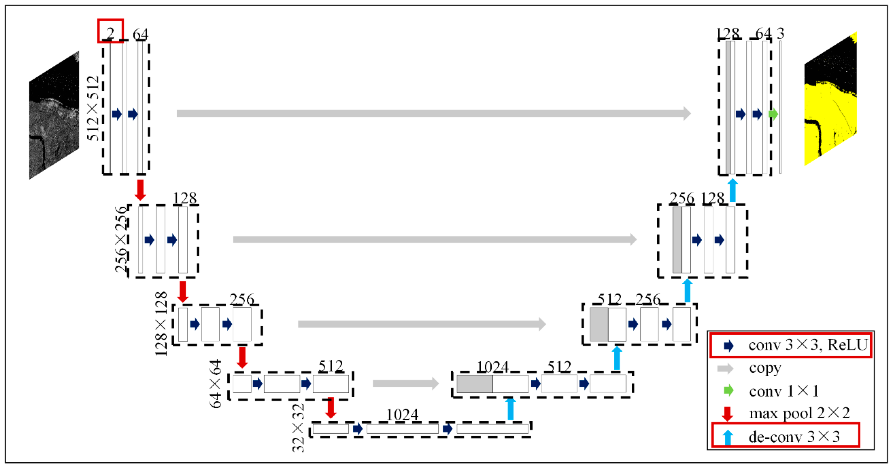
2.1. Architecture of U-Net
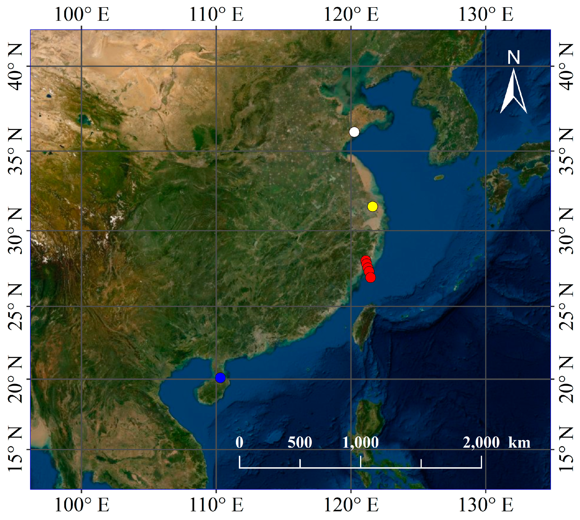
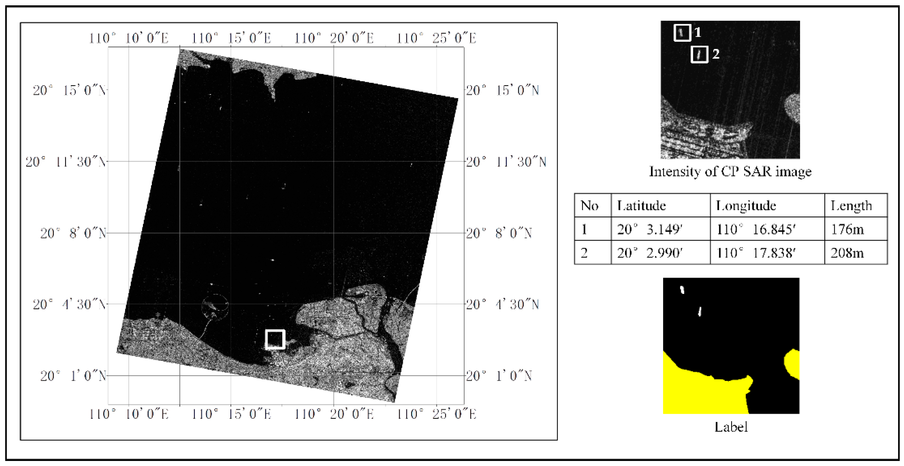
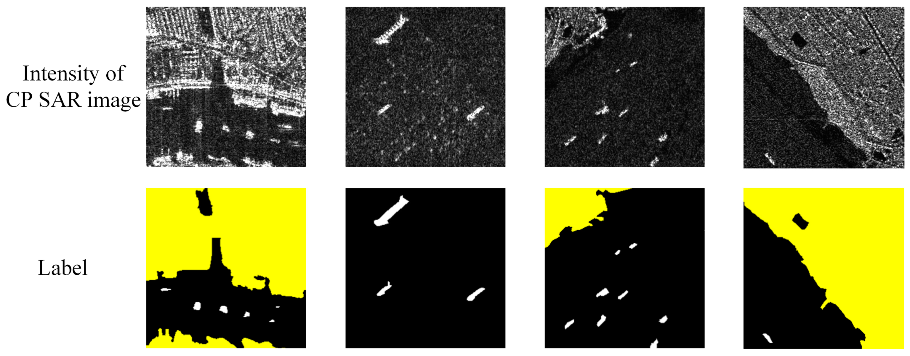
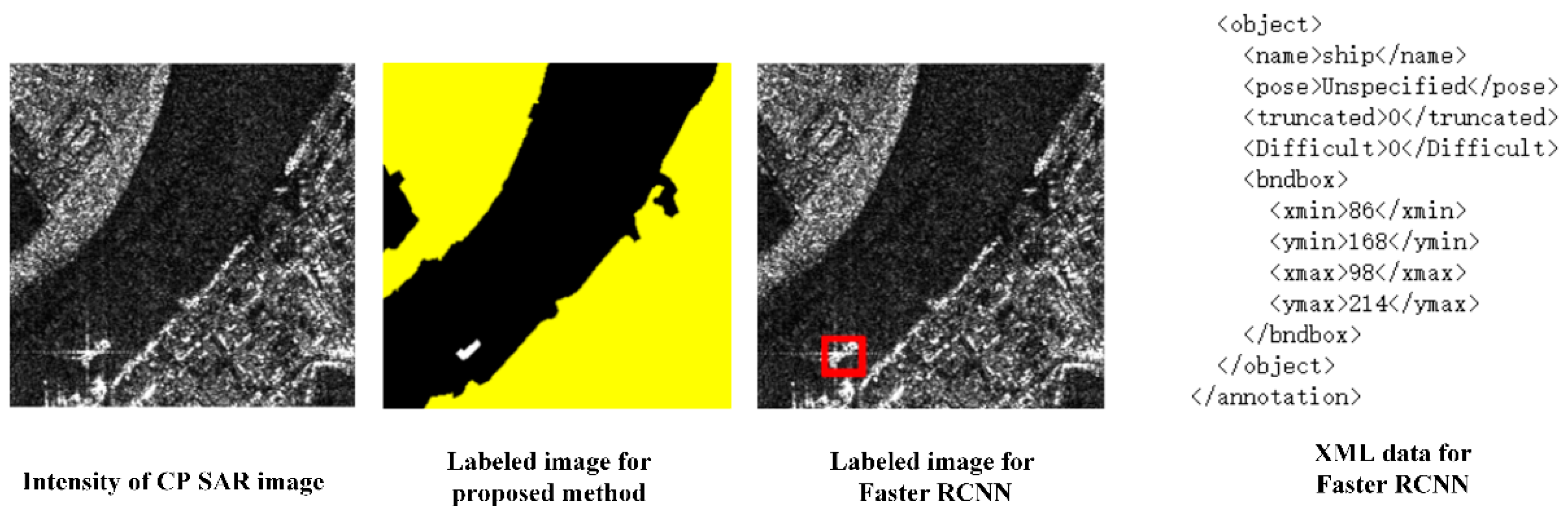
2.2. Data
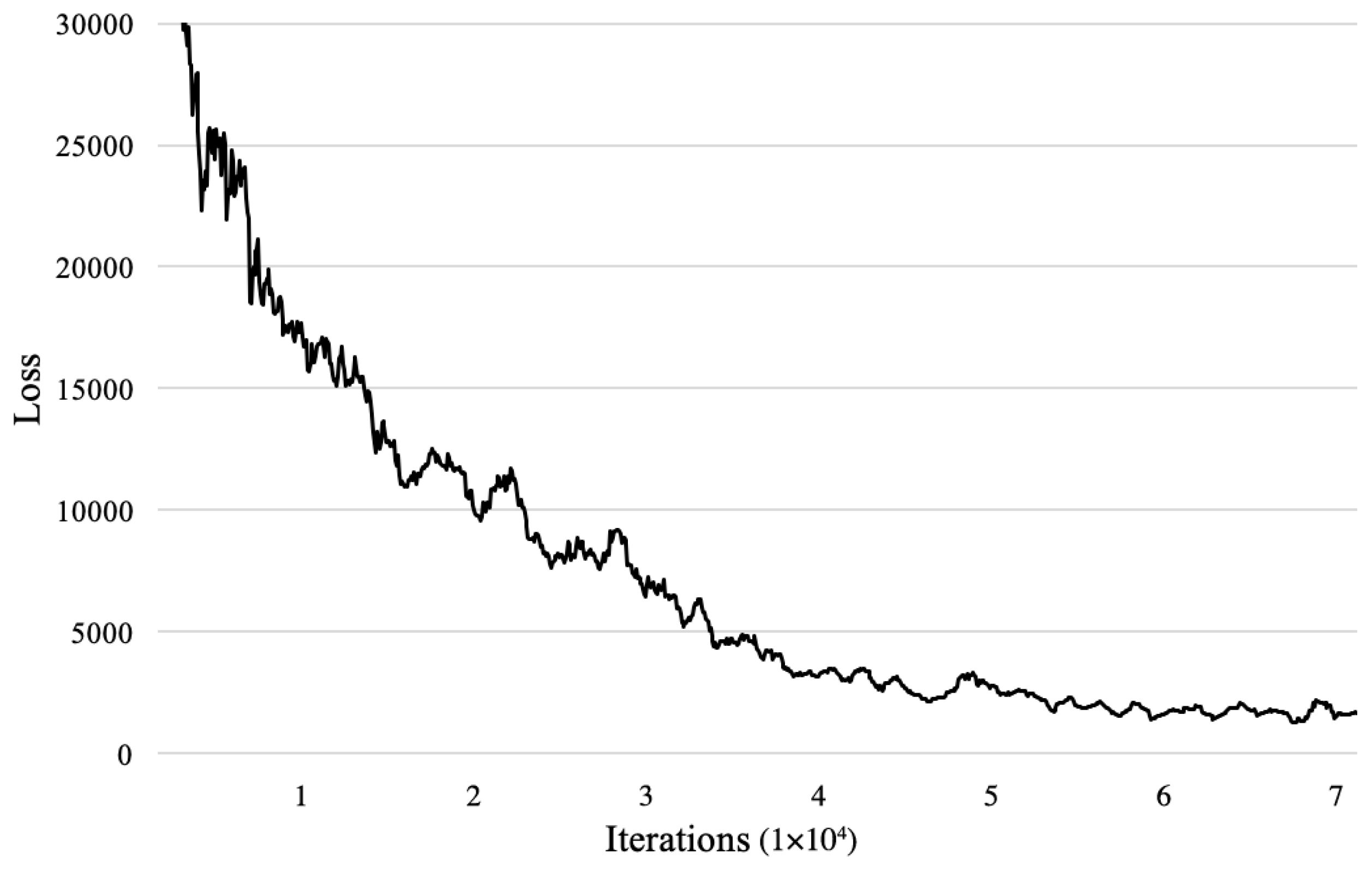
2.3. Training
2.4. Validation
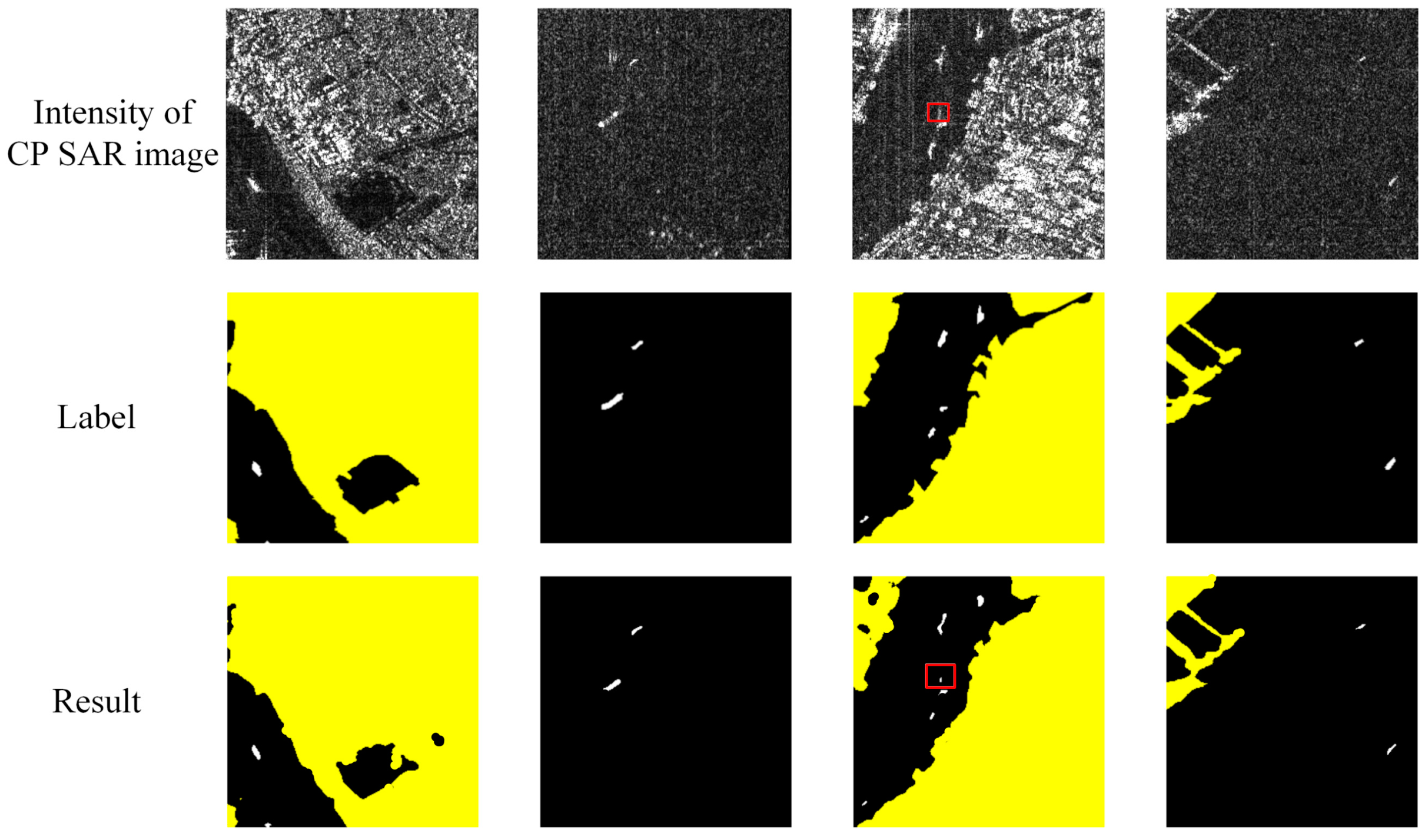
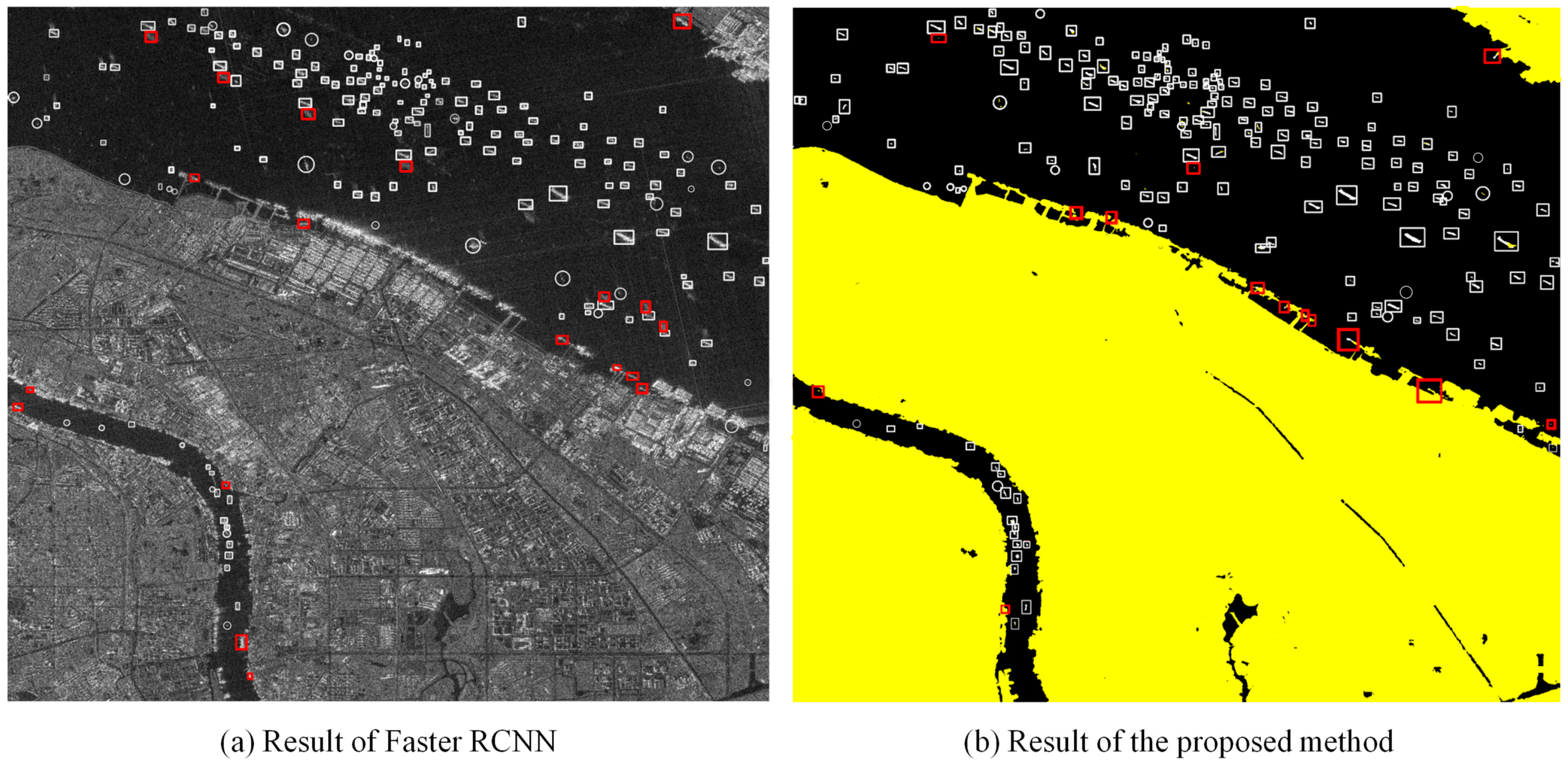
3. Results
4. Discussion
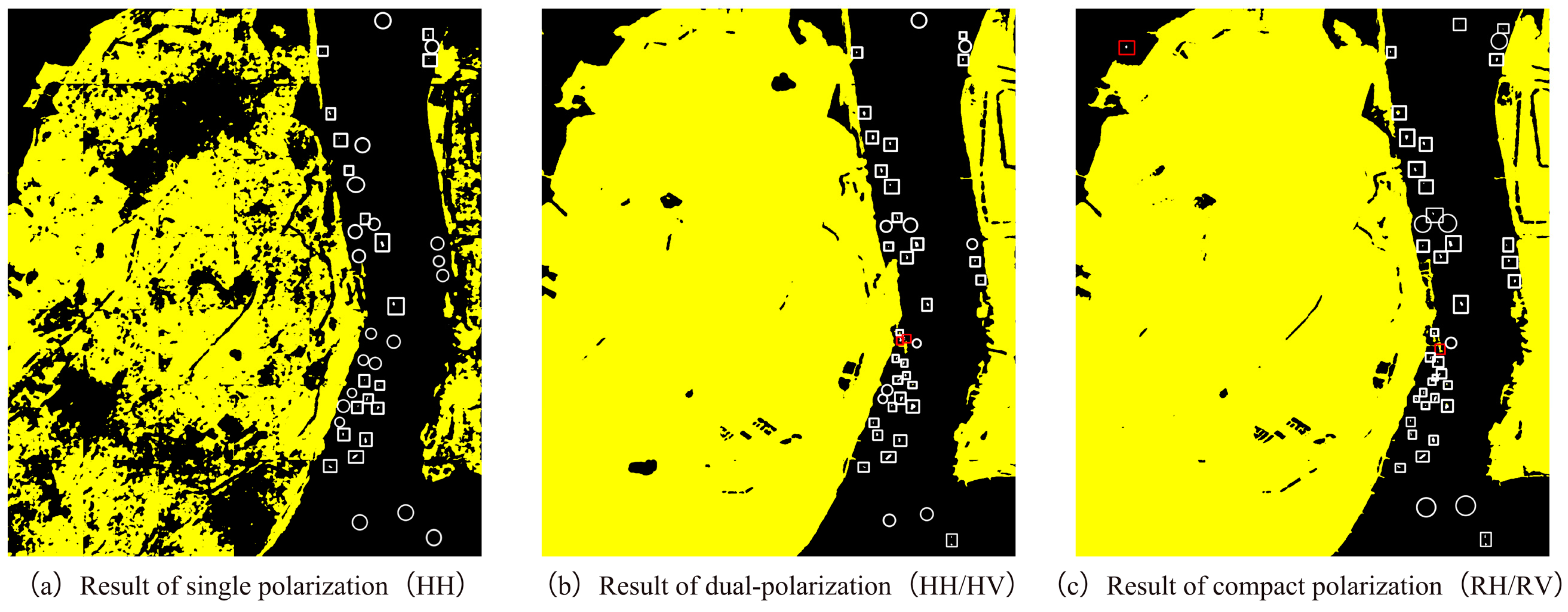
4.1. Comparison among Different Polarization Modes
4.2. Comparison among Different Networks based on U-Net
4.3. Validation
5. Conclusions
Author Contributions
Acknowledgments
Conflicts of Interest
References
- Charbonneau, F.; Brisco, B.; Raney, R. Compact polarimetry overview and applications assessment. Can. J. Remote Sens. 2010, 36, 298–315. [Google Scholar] [CrossRef]
- Zhang, B.; Li, X.; Perrie, W.; Garcia-Pineda, O. Compact polarimetric synthetic aperture radar for marine oil platform and slick detection. IEEE Trans. Geosci. Remote Sens. 2017, 55, 1407–1423. [Google Scholar] [CrossRef]
- Souyris, J.C.; Mingot, S. Polarimetry based on one transmitting and two receiving polarizations: The pi/4 mode. In Proceedings of the IEEE IGARSS, Toronto, ON, Canada, 24–28 June 2002; pp. 629–631. [Google Scholar]
- Stacy, N.; Preiss, M. Compact polarimetric analysis of X-band SAR data. In Proceedings of the EUSAR, Dresden, Germany, 16–18 May 2006. [Google Scholar]
- Raney, R. Comments on hybrid-polarity SAR architecture. In Proceedings of the IEEE IGARSS, Barcelona, Spain, 23–27 July 2007; pp. 2229–2231. [Google Scholar]
- Chin, G.; Brylow, S.; Foote, M.; Garvin, J.; Kasper, J.; Keller, J.; Litvak, M.; Mitrofanov, I.; Paige, D.; Raney, K.; et al. Lunar Reconnaissance Orbiter overview: The instrument suite and mission. Space Sci. Rev. 2007, 129, 391–419. [Google Scholar] [CrossRef]
- Goswami, J.; Annadurai, M. Chandrayaan-1: India’s first planetary science mission to the moon. Curr. Sci. India 2009, 96, 486–490. [Google Scholar]
- Atteia Allah, G. On the Use of Hybrid Compact Polarimetric SAR for Ship Detection. Ph.D. Thesis, University of Calgary, Calgary, AB, Canada, 5 December 2014; p. 170. [Google Scholar] [CrossRef]
- Souyris, J.; Imbo, P.; Fjortoft, R. Compact polarimetry based on symmetry properties of geophysical media: The π/4 mode. IEEE Trans. Geosci. Remote Sens. 2005, 43, 634–646. [Google Scholar] [CrossRef]
- Collins, M.; Denbina, M.; Atteia, G. On the reconstruction of quad-pol SAR data from compact polarimetry data for ocean target detection. IEEE Trans. Geosci. Remote Sens. 2013, 51, 591–600. [Google Scholar] [CrossRef]
- Nord, M.; Ainsworth, T. Comparison of compact polarimetric synthetic aperture radar modes. IEEE Trans. Geosci. Remote Sens. 2009, 47, 174–188. [Google Scholar] [CrossRef]
- Yin, J.; Yang, J.; Zhang, X. On the ship detection performance with compact polarimetry. In Proceedings of the IEEE RADAR, Chengdu, China, 24–27 October 2011; pp. 675–680. [Google Scholar]
- Xu, L.; Zhang, H.; Wang, C. Compact polarimetric SAR ship detection with m-δ decomposition using visual attention model. Remote Sens. 2016, 8, 751. [Google Scholar] [CrossRef]
- Shirvany, R.; Chabert, M.; Tourneret, J. Ship and oils-pill detection using the degree of polarization in linear and hybrid/compact dual-pol SAR. IEEE J. Sel. Top. Appl. Earth Observ. Remote Sens. 2012, 5, 885–892. [Google Scholar] [CrossRef]
- Li, H.; Perrie, W.; He, Y.; Lehner, S.; Brusch, S. Target detection on the ocean with the relative phase of compact polarimetry SAR. IEEE Trans. Geosci. Remote Sens. 2013, 51, 3299–3305. [Google Scholar] [CrossRef]
- Fan, Q.; Chen, F.; Cheng, M.; Wang, C.; Li, J. A modified framework for ship detection from compact polarization SAR image. In Proceedings of the IEEE IGARSS, Valencia, Spain, 22–27 July 2018; pp. 3539–3542. [Google Scholar]
- Liu, C.; Vachon, P.W.; English, R.A.; Sandirasegaram, N. Ship Detection Using RADARSAT-2 Fine Quad Mode and Simulated Compact Polarimetry Data; Defence R&D Canada: Ottawa, ON, Canada, 2009; Tech. Rep. DRDC-O-TM-2009-285.
- Atteia, G.; Collins, M. On the use of compact polarimetric SAR for ship detection. ISPRS J. Photogramm. Remote Sens. 2013, 80, 1–9. [Google Scholar] [CrossRef]
- Denbina, M.; Collins, M.J. Iceberg detection using compact polarimetric synthetic aperture radar. Atmos. Ocean. 2012, 50, 437–446. [Google Scholar] [CrossRef]
- Yin, J.; Yang, J.; Zhou, Z.; Song, J. The extended Bragg scattering model-based method for ship and oil-spill observation using compact polarimetric SAR. IEEE J. Sel. Top. Appl. Earth Observ. Remote Sens. 2014, 8, 3760–3772. [Google Scholar] [CrossRef]
- Gao, G.; Gao, S.; He, J.; Li, G. Ship detection using compact polarimetric SAR based on the notch filter. IEEE Trans. Geosci. Remote Sens. 2018, 56, 5380–5393. [Google Scholar] [CrossRef]
- Chang, Y.L.; Anagaw, A.; Chang, L.; Wang, Y.C.; Hsiao, C.; Lee, W. Ship detection based on YOLOv2 for SAR imagery. Remote Sens. 2019, 11, 786. [Google Scholar] [CrossRef]
- Kang, M.; Ji, K.; Leng, X.; Lin, Z. Contextual region-based convolutional neural network with multilayer fusion for SAR ship detection. Remote Sens. 2017, 9, 860. [Google Scholar] [CrossRef]
- Wang, Y.; Wang, C.; Zhang, H. Combining a single shot multibox detector with transfer learning for ship detection using sentinel-1 SAR images. Remote Sens. Lett. 2018, 9, 780–788. [Google Scholar] [CrossRef]
- Crisp, D.J. The State-of-the-Art in Ship Detection in Synthetic Aperture Radar Imagery; Defence Science and Technology Organisation Salisbury (Australia) Info Sciences Lab: Edinburgh, Australia, 2004. [Google Scholar]
- Iervolino, P.; Guida, R. A novel ship detector based on the generalized-likelihood ratio test for SAR imagery. IEEE J. Sel. Top. Appl. Earth Observ. Remote Sens. 2017, 10, 3616–3630. [Google Scholar] [CrossRef]
- Leng, X.; Ji, K.; Yang, K.; Zou, H. A bilateral CFAR algorithm for ship detection in SAR images. IEEE Geosci. Sens. Lett. 2015, 12, 1536–1540. [Google Scholar] [CrossRef]
- Greidanus, H.; Alvarez, M.; Santamaria, C.; Thoorens, F.; Kourti, N.; Argentieri, P. The SUMO ship detector algorithm for satellite radar images. Remote Sens. 2017, 9, 246. [Google Scholar] [CrossRef]
- Touzi, R. On the use of polarimetric SAR data for ship detection. In Proceedings of the IEEE IGARSS, Hamburg, Germany, 28 June–2 July 1999; pp. 812–814. [Google Scholar]
- Liu, C.; Vachon, P.W.; Geling, G.W. Improved ship detection using polarimetric SAR data. In Proceedings of the IEEE IGARSS, Anchorage, AK, USA, 20–24 September 2004; pp. 1800–1803. [Google Scholar]
- Nunziata, F.; Migliaccio, M.; Brown, C.E. Reflection symmetry for polarimetric observation of manmade metallic targets at sea. IEEE J. Oceanic Eng. 2012, 37, 384–394. [Google Scholar] [CrossRef]
- Marino, A. A notch filter for ship detection with polarimetric SAR data. IEEE J. Sel. Top. Appl. Earth Observ. Remote Sens. 2013, 6, 1219–1232. [Google Scholar] [CrossRef]
- Long, J.; Shelhamer, E.; Darrell, T. Fully convolutional networks for semantic segmentation. In Proceedings of the CVPR, Boston, MA, USA, 7–13 June 2015; pp. 8–10. [Google Scholar]
- Kampffmeyer, M.; Salberg, A.B.; Jenssen, R. Semantic segmentation of small objects and modeling of uncertainty in urban remote sensing images using deep convolutional neural networks. In Proceedings of the CVPRW, Las Vegas, NV, USA, 27–30 June 2016; pp. 680–688. [Google Scholar]
- Vijay, B.; Kendall, A.; Cipolla, R. SegNet: A deep convolutional encoder-decoder architecture for image segmentation. arXiv 2015, arXiv:1511.00561. [Google Scholar]
- Ronneberger, O.; Fischer, P.; Brox, T. U-net: Convolutional networks for biomedical image segmentation. In Proceedings of the MICCAI, Munich, Germany, 5–9 October 2015; pp. 234–241. [Google Scholar]
- Wei, S.; Zhang, H.; Wang, C.; Wang, Y.; Xu, L. Multi-temporal SAR data large-scale crop mapping based on U-Net model. Remote Sens. 2019, 11, 68. [Google Scholar] [CrossRef]
- Zhang, Z.; Liu, Q.; Wang, Y. Road extraction by deep residual u-net. IEEE Geosci. Remote Sens. Lett. 2018, 15, 749–753. [Google Scholar] [CrossRef]
- Huang, J.; Rathod, V.; Sun, C.; Zhu, M.; Korattikara, A.; Fathi, A.; Fischer, I.; Wojna, Z.; Song, Y.; Guadarrama, S.; et al. Speed/accuracy trade-offs for modern convolutional object detectors. In Proceedings of the CVPR, Hawaii, HI, USA, 21–26 July 2017; pp. 7310–7311. [Google Scholar]
- Shelhamer, E.; Long, J.; Darrell, T. Fully convolutional networks for semantic segmentation. IEEE Trans. Pattern Anal. Mach. Intell. 2017, 39, 640–651. [Google Scholar] [CrossRef] [PubMed]
- Sun, J.; Yu, W.; Deng, Y. The SAR payload design and performance for the GF-3 mission. Sensors 2017, 17, 2419. [Google Scholar] [CrossRef]
- Kang, W.; Xiang, Y.; Wang, F.; Wan, L.; You, H. Flood detection in Gaofen-3 SAR images via fully convolutional networks. Sensors 2018, 18, 2915. [Google Scholar] [CrossRef]
- An, Q.; Pan, Z.; You, H. Ship detection in Gaofen-3 SAR images based on sea clutter distribution analysis and deep convolutional neural network. Sensors 2018, 18, 334. [Google Scholar] [CrossRef]
- Chang, Y.; Li, P.; Yang, J.; Zhao, J.; Zhao, L.; Shi, L. Polarimetric calibration and quality assessment of the GF-3 satellite images. Sensors 2018, 18, 403. [Google Scholar] [CrossRef]
- Liu, J.; Qiu, X.; Hong, W. Automated ortho-rectified SAR image of GF-3 satellite using Reverse-Range-Doppler method. In Proceedings of the IEEE IGARSS, Beijing, China, 10–15 July 2016; pp. 4445–4448. [Google Scholar]
- Zhang, Q. System Design and Key Technologies of the GF-3 Satellite. Acta Geod. Cartogr. Sin. 2017, 46. [Google Scholar] [CrossRef]
- Wang, Y.; Wang, C.; Zhang, H.; Dong, Y.; Wei, S. A SAR dataset of ship detection for deep learning under complex backgrounds. Remote Sens. 2019, 11, 765. [Google Scholar] [CrossRef]
- Li, J.; Qu, C.; Shao, J. Ship detection in SAR images based on an improved faster R-CNN. In Proceedings of the 2017 BIGSARDATA, Beijing, China, 13–14 November 2017; pp. 1–6. [Google Scholar]
- Huang, X.; Yang, W.; Zhang, H.; Xia, G.S. Automatic ship detection in SAR images using multi-scale heterogeneities and an a Contrario decision. Remote Sens. 2015, 7, 7695–7711. [Google Scholar] [CrossRef]
- Abadi, M.; Agarwal, A.; Barham, P.; Brevdo, E.; Chen, Z.; Citro, C.; Corrado, G.S.; Davis, A.; Dean, J.; Devin, M.; et al. Tensorflow: Large-scale machine learning on heterogeneous distributed systems. arXiv 2016, arXiv:1603.04467. [Google Scholar]
- Kingma, D.P.; Ba, J. Adam: A method for stochastic optimization. arXiv 2014, arXiv:1412.6980. [Google Scholar]
- Faster RCNN. Available online: https://github.com/smallcorgi/Faster-RCNN_TF (accessed on 18 April 2018).
- Simonyan, K.; Zisserman, A. Very deep convolutional networks for large-scale image recognition. In Proceedings of the ICLR, San Diego, CA, USA, 7–9 May 2015. [Google Scholar]
- Everingham, M.; Gool, L.V.; Williams, C.K.I.; Winn, J.; Zisserman, A. The pascal visual object classes (VOC) challenge. Int. J. Comput. Vis. 2010, 88, 303–338. [Google Scholar] [CrossRef]
- LabelImg. Available online: https://github.com/tzutalin/labelImg (accessed on 18 April 2018).
- He, K.; Zhang, X.; Ren, S.; Sun, J. Deep residual learning for image recognition. In Proceedings of the CVPR, Las Vegas, NV, USA, 27–30 June 2016; pp. 770–778. [Google Scholar]
- Wang, P.; Chen, P.; Yuan, Y.; Liu, D.; Huang, Z.; Hou, X.; Cottrell, G. Understanding convolution for semantic segmentation. In Proceedings of the 2018 IEEE WACV, Lake Tahoe, NV, USA, 12–15 March 2018; pp. 1451–1460. [Google Scholar]
- Vachon, P.W.; Campbell, J.; Bjerkelund, C.; Dobson, F.; Rey, M. Ship detection by the RADARSAT SAR: Validation of detection model predictions. Can. J. Remote Sens. 1997, 23, 48–59. [Google Scholar] [CrossRef]
- Vachon, P.W.; Thomas, S.J.; Cranton, J.; Edel, H.R.; Henschel, M.D. Validation of ship detection by the RADARSAT Synthetic Aperture Radar and the Ocean Monitoring Workstation. Can. J. Remote Sens. 2000, 26, 200–212. [Google Scholar] [CrossRef]
- Vachon, P.W.; English, R.A.; Wolfe, J. Validation of RADARSAT-1 vessel signatures with AISLive data. Can. J. Remote Sens. 2007, 33, 20–26. [Google Scholar] [CrossRef]
- Vachon, P.W.; Kabatoff, C.; Quinn, R. Operational ship detection in Canada using RADARSAT. In Proceedings of the IEEE IGARSS, Quebec City, QC, Canada, 13–18 July 2014; pp. 998–1001. [Google Scholar]


| No | Type 1 | Input 2 | Filters | Size/Stride | Output 2 |
|---|---|---|---|---|---|
| 1 | conv | 512 × 512 × 2 | 64 | 3 × 3/1 | 512 × 512 × 64 |
| 2 | conv | 512 × 512 × 64 | 64 | 3 × 3/1 | 512 × 512 × 64 |
| 3 | max | 512 × 512 × 64 | 2 × 2/2 | 256 × 256 × 64 | |
| 4 | conv | 256 × 256 × 64 | 128 | 3 × 3/1 | 256 × 256 × 128 |
| 5 | conv | 256 × 256 × 128 | 128 | 3 × 3/1 | 256 × 256 × 128 |
| 6 | max | 256 × 256 × 128 | 2 × 2/2 | 128 × 128 × 128 | |
| 7 | conv | 128 × 128 × 128 | 256 | 3 × 3/1 | 128 × 128 × 256 |
| 8 | conv | 128 × 128 × 256 | 256 | 3 × 3/1 | 128 × 128 × 256 |
| 9 | max | 128 × 128 × 256 | 2 × 2/2 | 64 × 64 × 256 | |
| 10 | conv | 64 × 64 × 256 | 512 | 3 × 3/1 | 64 × 64 × 512 |
| 11 | conv | 64 × 64 × 512 | 512 | 3 × 3/1 | 64 × 64 × 512 |
| 12 | max | 64 × 64 × 512 | 2 × 2/2 | 32 × 32 × 512 | |
| 13 | conv | 32 × 32 × 512 | 1024 | 3 × 3/1 | 32 × 32 × 1024 |
| 14 | conv | 32 × 32 × 1024 | 1024 | 3 × 3/1 | 32 × 32 × 1024 |
| 15 | de_conv | 32 × 32 × 1024 | 512 | 3 × 3/2 | 64 × 64 × 512 |
| 16 | concat | 64 × 64 × 512 | 64 × 64 × 1024 | ||
| 17 | conv | 64 × 64 × 1024 | 512 | 3 × 3/1 | 64 × 64 × 512 |
| 18 | conv | 64 × 64 × 512 | 512 | 3 × 3/1 | 64 × 64 × 512 |
| 19 | de_conv | 64 × 64 × 512 | 256 | 3 × 3/2 | 128 × 128 × 256 |
| 20 | concat | 128 × 128 × 256 | 128 × 128 × 512 | ||
| 21 | conv | 128 × 128 × 512 | 256 | 3 × 3/1 | 128 × 128 × 256 |
| 22 | conv | 128 × 128 × 256 | 256 | 3 × 3/1 | 128 × 128 × 256 |
| 23 | de_conv | 128 × 128 × 256 | 128 | 3 × 3/2 | 256 × 256 × 128 |
| 24 | concat | 256 × 256 × 128 | 256 × 256 × 256 | ||
| 25 | conv | 256 × 256 × 256 | 128 | 3 × 3/1 | 256 × 256 × 128 |
| 26 | conv | 256 × 256 × 128 | 128 | 3 × 3/1 | 256 × 256 × 128 |
| 27 | de_conv | 256 × 256 × 128 | 64 | 3 × 3/2 | 512 × 512 × 64 |
| 28 | concat | 512 × 512 × 64 | 512 × 512 × 128 | ||
| 29 | conv | 512 × 512 × 128 | 64 | 3 × 3/1 | 512 × 512 × 64 |
| 30 | conv | 512 × 512 × 64 | 64 | 3 × 3/1 | 512 × 512 × 64 |
| 31 | conv | 512 × 512 × 64 | 3 | 1 × 1/1 | 512 × 512 × 3 |
| Image Number | Region | Nominal Resolution (m) | Acquisition Mode | Acquired Time (yyyy-mm-dd) | Incidence Angle (NearRange/FarRange) (degree) | Pixel Spacing (Rng/Az) # (m) |
|---|---|---|---|---|---|---|
| 1 | Taizhou Area | 8 | Ascending | 2016-12-26 | 33.6833/35.6152 | 2.2484/5.1995 |
| 2 | Taizhou Area | 8 | Ascending | 2016-12-26 | 33.6830/35.6150 | 2.2484/5.1994 |
| 3 | Taizhou Area | 8 | Ascending | 2016-12-26 | 33.6828/35.6147 | 2.2484/5.2000 |
| 4 | Taizhou Area | 8 | Ascending | 2016-12-26 | 33.6827/35.6144 | 2.2484/5.1998 |
| 5 | Taizhou Area | 8 | Ascending | 2016-12-26 | 33.6836/35.6156 | 2.2484/5.1997 |
| 6 | Shanghai Area | 8 | Ascending | 2016-12-31 | 28.3065/30.6847 | 2.2484/4.7303 |
| 7 | Qingdao Area | 8 | Ascending | 2017-10-12 | 36.7626/38.1709 | 2.2484/5.2981 |
| 8 | Haikou Area | 8 | Descending | 2017-09-27 | 36.7564/38.1533 | 2.2484/4.7219 |
| Method | TP | FP | FN | Pf (%) | Precision (%) | Recall (%) | F1 Score |
|---|---|---|---|---|---|---|---|
| Standard CFAR | 609 | 307 | 74 | 33.52 | 66.48 | 89.17 | 0.762 |
| Faster RCNN | 565 | 95 | 124 | 14.39 | 85.61 | 82.00 | 0.838 |
| U-Net | 622 | 53 | 67 | 7.85 | 92.15 | 90.28 | 0.912 |
| Combination Modes | Channels | Pf (%) | Precision (%) | Recall (%) | F1 score | mIoU |
|---|---|---|---|---|---|---|
| Single polarization | HH | 6.86 | 93.14 | 49.87 | 0.650 | 0.601 |
| Linear dual-polarization | HH+HV | 8.22 | 91.88 | 81.37 | 0.863 | 0.734 |
| Compact polarization | RH+RV | 7.85 | 92.15 | 90.28 | 0.912 | 0.817 |
| Methods | Pf (%) | Precision (%) | Recall (%) | F1 Score | mIoU |
|---|---|---|---|---|---|
| Proposed (10 layers) | 7.85 | 92.15 | 90.28 | 0.912 | 0.817 |
| U-Net+Res-Block (32 layers) | 7.63 | 92.37 | 91.36 | 0.919 | 0.826 |
| U-Net+Dilated Convolutional Kernel | 12.11 | 87.89 | 89.21 | 0.885 | 0.802 |
© 2019 by the authors. Licensee MDPI, Basel, Switzerland. This article is an open access article distributed under the terms and conditions of the Creative Commons Attribution (CC BY) license (http://creativecommons.org/licenses/by/4.0/).
Share and Cite
Fan, Q.; Chen, F.; Cheng, M.; Lou, S.; Xiao, R.; Zhang, B.; Wang, C.; Li, J. Ship Detection Using a Fully Convolutional Network with Compact Polarimetric SAR Images. Remote Sens. 2019, 11, 2171. https://0-doi-org.brum.beds.ac.uk/10.3390/rs11182171
Fan Q, Chen F, Cheng M, Lou S, Xiao R, Zhang B, Wang C, Li J. Ship Detection Using a Fully Convolutional Network with Compact Polarimetric SAR Images. Remote Sensing. 2019; 11(18):2171. https://0-doi-org.brum.beds.ac.uk/10.3390/rs11182171
Chicago/Turabian StyleFan, Qiancong, Feng Chen, Ming Cheng, Shenlong Lou, Rulin Xiao, Biao Zhang, Cheng Wang, and Jonathan Li. 2019. "Ship Detection Using a Fully Convolutional Network with Compact Polarimetric SAR Images" Remote Sensing 11, no. 18: 2171. https://0-doi-org.brum.beds.ac.uk/10.3390/rs11182171