Structural 3D Reconstruction of Indoor Space for 5G Signal Simulation with Mobile Laser Scanning Point Clouds


1
Shenzhen Key Laboratory of Spatial Smart Sensing and Services & The Key Laboratory for Geo-Environment Monitoring of Coastal Zone of the National Administration of Surveying, Mapping and GeoInformation & College of Information Engineering, Shenzhen University, Nanhai Road 3688, Shenzhen 518060, China
2
State Key Laboratory of Information Engineering in Surveying, Mapping and Remote Sensing, Wuhan University, Wuhan 430079, China
*
Author to whom correspondence should be addressed.
Remote Sens. 2019, 11(19), 2262; https://0-doi-org.brum.beds.ac.uk/10.3390/rs11192262
Submission received: 2 September 2019
/
Revised: 23 September 2019
/
Accepted: 23 September 2019
/
Published: 27 September 2019
(This article belongs to the Special Issue Remote Sensing based Building Extraction)
Abstract
:3D modelling of indoor environment is essential in smart city applications such as building information modelling (BIM), spatial location application, energy consumption estimation, and signal simulation, etc. Fast and stable reconstruction of 3D models from point clouds has already attracted considerable research interest. However, in the complex indoor environment, automated reconstruction of detailed 3D models still remains a serious challenge. To address these issues, this paper presents a novel method that couples linear structures with three-dimensional geometric surfaces to automatically reconstruct 3D models using point cloud data from mobile laser scanning. In our proposed approach, a fully automatic room segmentation is performed on the unstructured point clouds via multi-label graph cuts with semantic constraints, which can overcome the over-segmentation in the long corridor. Then, the horizontal slices of point clouds with individual room are projected onto the plane to form a binary image, which is followed by line extraction and regularization to generate floorplan lines. The 3D structured models are reconstructed by multi-label graph cuts, which is designed to combine segmented room, line and surface elements as semantic constraints. Finally, this paper proposed a novel application that 5G signal simulation based on the output structural model to aim at determining the optimal location of 5G small base station in a large-scale indoor scene for the future. Four datasets collected using handheld and backpack laser scanning systems in different locations were used to evaluate the proposed method. The results indicate our proposed methodology provides an accurate and efficient reconstruction of detailed structured models from complex indoor scenes.
1. Introduction
Three-dimensional (3D) reconstruction of the indoor environment has received significant attention due to the development of smart cities. However, the automation of generating high-quality models remains to be a challenging issue due to the complexities of the indoor environment. The industry foundation classes (IFC) defines building information modelling (BIM) as having rich semantic information, 3D structural information, spatial relationships, and interoperable geometry [1]. BIM has been used in a number of applications, such as indoor navigation [2,3], space management [4,5], energy simulation [6] and real-time emergency response [7,8]. Primary indoor locations utilizing BIM include indoor offices, parking lots, and commercial establishments, which are commonly comprised of basic elements, such as the ceilings, floors, walls, windows, doors, and pillars, and not objects, such as furniture. 3D Indoor models are often generated manually by creating geometric representations using point cloud data and commercial software. This often requires significant investment in time and in training personnel [9]. To accelerate the efficiency of data acquisition and improve the automation of reconstructed models, various laser scanning technologies and automated modelling methods have been developed. Over the past few years, terrestrial laser scanning (TLS) has been used to obtain high-quality data in the indoor scene, but often suffers from low mapping efficiency due to laborious scan station resetting, protracted registration procedures, and high costs. Thus, its application has excluded large-scale indoor data acquisition. RGBD panorama is acquired by a camera and a depth sensor [10], with added advantages of affordability and convenience of use. However, the image distorted and noisy that lead to difficultly build accurate models in large scale scenes. With the development of the simultaneous localization and mapping (SLAM), various types of mobile laser scanning (MLS) devices have been used for data acquisition, such as handheld, backpack, push-cart and robot mobile laser scanners. MLS systems can obtain point clouds by moving from different spaces and measure from different locations. The easy-to-use and affordable indoor MLS systems are mostly used for data acquisition of large indoor scenes [11]. While MLS ensures good coverage for indoor environment mapping, the data can be affected by a number of factors (e.g., moving objects, multiple reflections, and dynamic occlusions) resulting in quality losses, which present serious challenges in model reconstruction.
Recently, numerous studies have focused on modelling the indoor environment. For example, some research [10,12,13,14,15,16,17,18,19,20,21,22] segmented the unstructured points clouds into individual rooms to provide a prior knowledge in building the indoor model. The over-segmentation often occurs in the spatial partition of long corridors [13,14], creating a substantial challenge when segmenting long corridors. Neoteric methods [9,15,22,23,24,25,26,27,28,29,30,31] have focused on extracting piecewise planar surfaces to construct the model. Although the results of room segmentation have been satisfactory, indoor models still are difficult to accurately reconstruct because of high levels of occlusion and noisy point cloud data, while still requiring interaction [22]. Large scale scene modelling based on surface elements has significant computational challenges. In order to increase computational efficiency, many line-based reconstructed methods have been proposed [32,33,34,35,36,37,38,39,40]. Their results have shown that line-based methods are efficient and effective, which can produce accurate and complete line segments. However, the reconstructed models are only represented in vector line structure without room semantic information, even when these elements are unconnected. Furthermore, a satisfactory solution for indoor interior reconstruction has not been developed due to the complexity of the indoor environment and unfiltered data noise.
In this study, a novel method is developed that combines line structures and 3D surface geometry to automatically build a 3D indoor model with detailed structural and semantic information using MLS point clouds. A fully automatic room segmentation was performed on unstructured point clouds via multi-label graph cuts, which can solve the over-segmentation in long corridors. Point cloud slices of individual rooms are transformed as a binary image, from which extraction, and regularization of line elements, aimed at improving the computational efficiency and structural accuracy. 3D structured models were reconstructed using multi-label graph cuts, and room segmentation and lines were used as semantic and structural constraints of 2D floorplan, with surfaces providing 3D geometric information. Finally, an innovative approach was employed using 5G signal simulation based on the reconstructed model, where the basic structural elements (e.g., windows, doors, pillars, walls, ceilings, and floors) have a critical effect on the signal transmission.
This study offers two major contributions. First, room segmentation was employed to semantically label the unstructured point clouds using multi-label graph cuts with semantic constraints of openings that can overcome the over-segmentation in corridors. Point cloud slices of individual rooms are transformed into images, which are then extracted and regularized into the floorplan lines. This innovation contributes to improving the efficiency and precision of extracting structural elements. Second, 3D structured models were reconstructed using multi-label graph cuts with room segmentation and 2D floorplan lines, and with 3D surfaces used as constraints. The resulting structured models provided room adjacency relationship, geometric characteristics, and semantic information, which are then applied to the signal simulation to provide the optimal location of the 5G small base station in indoor environment for future.
2. Related Work
In the last decade, various approaches designed for indoor modelling using 3D laser scanning have been developed, which mostly consisted of three fundamental steps: (1) room segmentation, (2) reconstruction of indoor space, and (3) indoor model application.
2.1. Room Segmentation
Room segmentation is key semantic information used in model reconstruction. Ikehata et al. [10] proposed the segmentation method of rooms, which repeated k-medoids algorithm to cluster sub-sampled pixels, the distance metric for clustering is based on a binary visibility vector of scanning center. Mura et al. [12] presented an approach that established a global affinity measure between cells by diffusion maps, and partitioned rooms by clustering 2D cells iteratively. Ochmann et al. [13] proposed a method that segmented indoor point clouds into individual rooms by the visibility-based and class-conditional probabilities, which based on initial knowledge of scans and scan positions; however, the over-segmentation occurs in long corridors. Turner et al. [14] proposed an approach that triangulated a 2D sampling of wall positions and separated these triangles into interior and exterior domains. The room segmentation can be obtained by Graph-cut in the triangulated map. However, these methods of room partition are limited to depend on TLS the scanning position, but not for MLS point clouds. Wang et al. [17] employed the hierarchical clustering method for partitioning rooms, which established diffusion maps to merge the over-segmented spaces. The method uses scan trajectories instead of scanner positions. Díaz-Vilariño et al. [18] proposed a method that used the timestamp information to determine the visible point clouds of each trajectory point and constructed the energy minimization function for global spatial optimization to complete individual room segmentation. Their method relies heavily on data quality and integrity and has been shown effective in simple scenarios. Li et al. [19] proposed a comprehensive segmentation method that is created by a morphological erosion and connectivity analysis methods on the floor space, which overcomes over-segmentation in long corridors. Similarly, Ochmann et al. [22] proposed a fully automatic room segmentation that performed visibility tests by the ray casting between point patches on surfaces to build visibility graph, and then the nodes of this graph are clustered by the Markov Clustering method [21].
2.2. Reconstruction of Indoor Space
Current methods for the reconstruction of indoor spaces are mainly based on the extraction of surfaces [9,15,22,23,24,25,26,27,28,29,30,31] and lines [32,33,34,35,36,37,38,39,40].
(1) Surface-Based Reconstruction
The accuracy of reconstruction models mostly depends on the extraction of surfaces. Bassier and Vergauwen [9] proposed an innovative approach to segment walls using the Conditional Random Field and concluded that the generated wall clusters were better than traditional region growing. Other researchers have also extracted unconnected planes from 3D point clouds [23,24], but only enabled visualization and excluded the spatial topological relationship. Monszpart et al. [25] proposed an effective approach to extract Regular Arrangements of Planes (RAP) from unstructured point clouds in rebuilding man-made scenes. However, the method requires long computing time for the reconstruction of large scenes. Awrangjeb et al. [26] proposed a novel 3D roof reconstruction technique that constructs an adjacency matrix to define the topological relationships among the detected roof planes, in addition, used the generated building models to detect 3D change in buildings. Xiao and Furukawa [27] employed constructive solid geometry (CSG) operations to generate volumetric wall model, which focused on the large-scale reconstruction without semantic information. To overcome this deficiency, Ochmann et al. [15] extracted the piece planar surfaces by the RANSAC approach [28], constructed partitions based on the wall surfaces, utilized the global optimization to reconstruct wall elements, and then finally built the volumetric model of single room by extruding the walls. However, the thickness of model walls was assigned a fixed threshold that led to significant errors. Mura et al. [29] extracted the permanent components used in constructing adjacent relations and partitions of 3D polyhedral cells. The final general three-dimensional interior model was reconstructed using multi-label to optimize cell selection; however, this method was only applied to small-scale scenes. Ochmann et al. [22] extracted wall candidates and formulated the optimization method to arrange volumetric wall entities to build the structural model. Reconstructing the model presents latent difficulties due to occlusion and clutter point clouds in the indoor environment. While this approach can reshape the model manually, its main limitation includes slanted walls, ceilings and floors, and detailed pillar reconstruction.
(2) Line-Based Reconstruction
Many researchers have also studied indoor reconstruction based on lines. Lin et al. [32] proposed a method where line segments can accurately be extracted from unorganized point clouds. However, the line elements remained completely isolated and devoid of information about topological relations. Similarly, Xia and Wang [33], Lu et al. [34] extracted unstructured line elements from point clouds. Liu et al. [35] proposed the FloorNet where a deep neural architecture can automatically reconstruct the floorplan from RGBD videos with camera poses. Extracting initial line structures from labeled points, Wang et al. [37] proposed a conditional Generative Adversarial Nets (cGAN) deep learning method to optimize the detected lines to rebuild line frameworks with structural representation in the cluttered indoor environment. Bauchet et al. [38] proposed an approach that extract flexibility on polygon shape, which better recover geometric patterns but still lacks topological information. Sui et al. [39] introduced an automatic method for extracting floorplans from slices that correct both normal vector and position to obtain accurate boundaries, which are then used in propagating to the other floors. However, the reconstructed models are only applicable for visualization and cannot be used for geometric manipulation. For the underground infrastructure, Novakovic et al. [40] extracted the 2D profile from the point cloud data of tunnel, built the spatial parameter model and simulated cargo tunnel pass.
2.3. Indoor Model Application
Previous studies have investigated the various applications of the BIM model. Díaz-Vilariño et al. [3] proposed an approach based on the BIM model that determined the optimal scan positions in planning the shortest route for an automatic robot visit. Boyes et al. [4] proposed the combined use of BIM and GIS for spatial data management (e.g., location queries). Tomasi et al. [5] introduced the use of the BIM model in computing for the optimal coverage of Wireless sensor networks (WSNs). Rafiee et al. [6] applied the methods transforming BIM model with geometric and semantic information into geo-referenced vector model for view and shadow analyses, which are useful in urban spatial planning. Tang and Kim [7] introduced a dynamic fire simulation based on the Fire Dynamics Simulator (FDS) and BIM model, which included simulation control, fire and smoke modelling, and occupant evacuation in the indoor environment. Boguslawski et al. [8] introduced that the route planning of indoor fire emergency based on BIM model. Thus, the indoor model reconstruction has become extremely valuable in urban development.
2.4. Summary
These surface-based reconstruction methods [9,15,22,23,24,25,26,27,28,29,30,31] mostly depend on the accuracy of surface extraction. In complex indoor scenes, the efficiency of surface extraction is low and contains excessive noise. Line-based reconstruction methods [32,33,34,35,36,37,38,39,40] can be used to completely represent the geometric information; however, these do not contain semantic information and adjacency relationship of rooms, leaving the reconstructed models to be useful only for visualization. In order to address the above shortcomings, we propose an innovative approach combining the rich structure of 2D lines with 3D geometry of surfaces to automatically build 3D structured models using MLS point cloud data. The output structural model presents novel applications in signal simulation, including the capability of providing optimal locations for 5G small base stations in the future.
3. Methodology
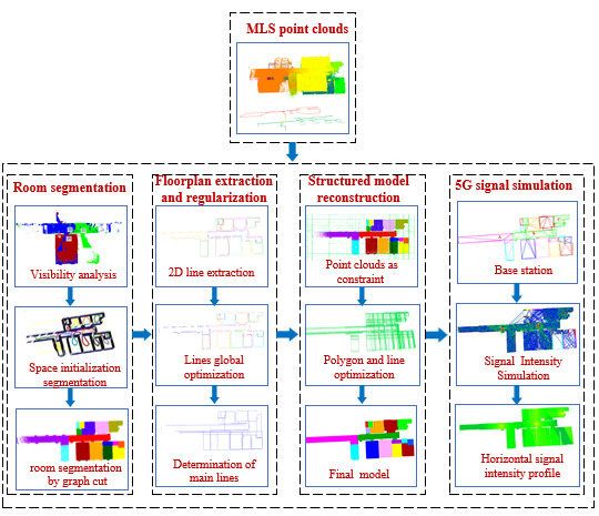
The complete flowchart is illustrated in Figure 1, showing the four key steps in the proposed methodology: room segmentation, floorplan extraction and regularization, structural model reconstruction, and 5G signal simulation. For the room segmentation, the door position and the simulated visible point clouds of sample trajectories are used to establish the initial space, while the global optimization of the indoor space is solved by the energy minimization function via multi-label graph cuts. For the floor extraction and regularization, the line elements are processed, which included the following steps: (1) the 3D point cloud slices are transformed into a binary image, and the line elements are extracted from the image; (2) the correction of line elements are based on global optimization; and, (3) similar lines are clustered to remove redundant line elements. The three-dimensional structural models are reconstructed via multi-label graph cuts, with room segmentation, 2D line elements, and 3D surfaces as semantic constraints. Finally, the signal intensity of 5G small base station is simulated using the structural models in the indoor environment.
3.1. Room Segmentation
The input of our approach, consists of unstructured point clouds and trajectories acquired from the mobile laser scanner system. In the indoor scene, every room has at least one door, representing a transition from one indoor space to another. For room segmentation, the position of detected doors and the simulated visible point clouds of sample trajectories are used to establish the initial space, while the global optimization of the indoor space is solved using the energy minimization function via multi-label graph cuts.
3.1.1. Detection of Openings
Since openings are generally attached to wall surfaces and as holes in the point clouds of wall surfaces, the extraction of doors and windows is based on the hierarchical relationship of plane-contour. The surfaces are first extracted based on the previous plane segmentation [31] (see wall surfaces illustrated in Figure 2a). The 3D point clouds of wall surfaces are projected into a 2D plane using the following conversion:
where are normal vectors of 3D plane; are vectors of the 3D plane coordinate axis that constituted the transformation matrix ; are coordinates of 3D plane; are the 2D coordinates of the transformed plane; and, is depth.
The 2D projected points are converted into a binary image, as shown in Figure 2b. For every binary image, morphological corrosion transformation is used to remove noise. The find-contour method [41] is then applied during the extraction of plane outline to get sets of contour points, such that every contour is independent. Afterward, the bounding boxes of contours are calculated. Based on the size of the bounding box, the contours are categorized into doors, windows, invalid. The invalid consists of holes resulting from occlusion and undetected openings. In our study, the template match method, which is implemented in the OpenCV library [42], is applied to extract undetected openings. (In Figure 2c, an extracted opening as the template that encircled in red; in Figure 2d, the identified doors are shaded in green). Compared with the previous method [31], the extracted opening boundaries are visually more defined. As for the extraction of pillars, the technique is similar to extracting openings.
3.1.2. Room-Space Segmentation
The segmentation of rooms is accomplished by first simulating the visible point clouds from the MLS trajectory based on the line-of-sight. The position of doors is then used to limit the range of visible point clouds and to partition the trajectory segments in establishing the initial space. Finally, similar visible points between scanning trajectories are automatically clustering using global optimization based on multi-label graph cuts.
Inspired by the previous room segmentation [31], the visibility analysis is that simulating the visible point clouds along sample trajectory of the MLS and the grid cells’ center point based on the line-of-sight. Instead of being dependent on segmented planes, the original point clouds are divided into uniform grids and the sampled point is one of every 200 trajectory points from the original trajectories. Figure 3 shows the flowchart, which illustrates the intersections between rays and all the other cells found along the line-of-sight. The points in the target cell are only visible if the point number of the cell where the ray passes through is within the threshold. Figure 4a shows the simulated visible point clouds of the three sample trajectories, some points are collected by different rooms due to the openings. Thus, the position of doors can be used to separate different spaces by limiting the range of visible points, as shown in Figure 4b.
The location of doors plays an important role in room segmentation. In our proposed methodology, the location of doors is used to subdivide the trajectories into initialized subspaces. Figure 5b illustrates how the trajectories are segmented by each door. Each trajectory segment corresponds to only one room, but not all rooms are depicted by a single segment. Trajectories in the same space have similar visible point clouds, so the individual room can be segmented, which regard as automatic clustering of similar visible point clouds by the global optimized method.
The global optimization of indoor spaces is performed by solving an energy minimization function via multi-label graph cuts. The optimization function consists of a unary and smooth term, which is expressed as Equation (2), where weight parameters are used in balancing the data term and the smooth term in the energy function. The initial trajectory is first segmented using the doors as positional constraints, then, its corresponding clustering spaces are determined by minimizing a predefined energy function.
Data term. is the sum of unary functions; and, is the difference in visual area between trajectory and every trajectory segment , which is expressed in Equation (3):
where is the label for the trajectory belonging to trajectory segment ; is the ideal value for the label ; is the ratio of the overlapping area between trajectory and each trajectory segment ; is the visual area of trajectory , and is the visual area of trajectory segment ; are the set of initial trajectory segments, where , . Lower values mean less penalty when assigning the sample trajectory point to the trajectory segment . The overlap between the visible area of two trajectory points is calculated using the number of the same index for visible cells.
Smoothness term. is the sum of binary functions and is used to regularize label by penalizing the assignment of different labels to adjacent trajectories, as defined by Equation (4):
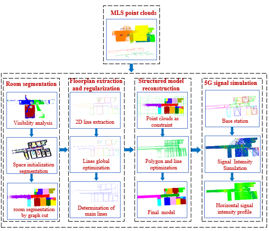
where is the sampled trajectory point; and let be as center point and get its k-nearest neighbor (KNN) trajectory points, ; are visible area of trajectory points and , respectively; is the distance between trajectory points and , is the overlapping ratio of visual area of trajectory points and ; is a distance threshold. The smoothness term indicates the penalty between adjacent trajectory points. If a pair of neighboring trajectory points belong to the same space, the smooth cost between them is 0; otherwise, this value is closer to 1 as the overlapping ratio is greater and the distance of the adjacent trajectory points is smaller. The smooth term can reduce the number of redundant spaces, thus solving the over-segmentation problem in long corridors for complex indoor environment. Again, the global optimization of the indoor space is solved by an energy minimization function via multi-label graph cuts [43,44,45] to automatically cluster similar visible point clouds. The room segmentation results are shown in Figure 6b.
3.2. Floorplan Extraction and Regularization
These methods [15,22,27,29] extracted mainly the piecewise planar surfaces to reconstruct indoor models. However, due to the complexity of the indoor environment, the quality of point clouds can suffer significantly from a number of factors such as moving objects, multiple reflections, and occlusions. Building high-accuracy indoor model automatically becomes complex, which may require interaction. Since lines are commonly used in expressing key information in modelling, line-based reconstruction ensures the efficiency and precision of the model. In this study, our method combines lines and surfaces in building the 3D structured model of the indoor scene. The extraction and regularization of lines are conducted prior to the reconstruction of the vector model with more detailed features.
3.2.1. Floorplan Line Extraction
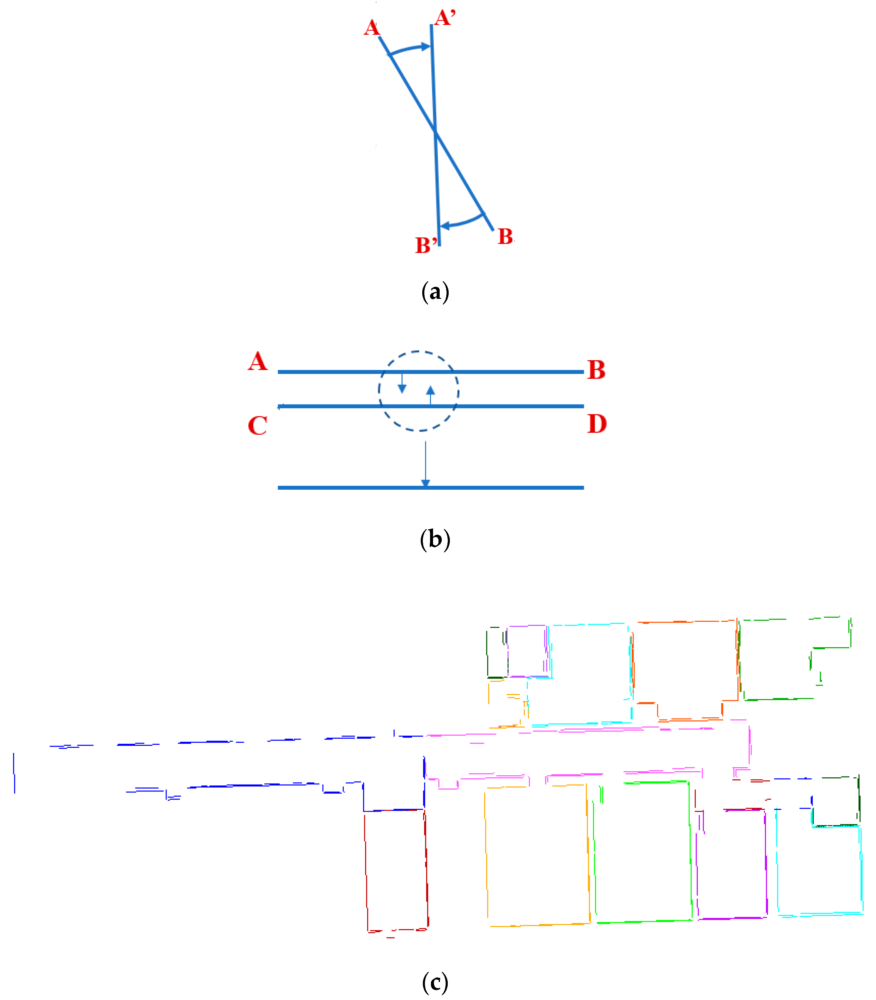
The horizontal slices of the point clouds with individual room are determined based on certain heights from the ceiling. Connectivity analysis is performed to filter outliers from the point cloud slicing (results are shown in Figure 7a). Line segments are then extracted based on the image gradient, which recovers detailed structural features and greatly improves computational efficiency. The point clouds of horizontal slices are converted into a binary image, as shown in Figure 7b, with a pixel size of 5 cm. We use the Line-Segment-Detector (LSD) [46] method to extract lines from the binary image, which region-growing method is applied to the image gradient clustering. The larger gradient is used as the seed point, while the given angle threshold is used as the growing condition. The line extraction results are shown in Figure 7c with the line elements of different rooms presented in varying colors.
3.2.2. Line Global Optimization
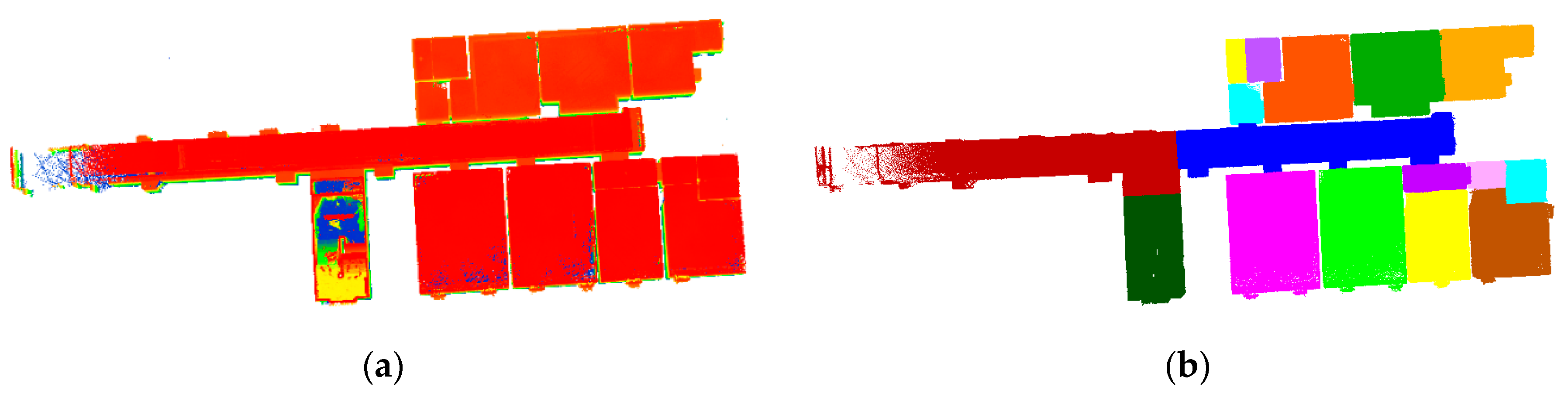
Figure 7c shows that the extracted initial lines are able to preserve detailed features. However, due to laser point clouds with information loss, holes, noise, etc., the extracted results mainly have four kinds of errors: angle deviation, distance deviation, excessive redundancy, and incomplete boundaries. Inspired the method [38], the angle and distance deviations of the line-segments are corrected by global optimization, as shown in Figure 8a,b. The problem is expressed as an energy function, as shown in Equation (5), which is minimized by g2o that called a general framework for graph optimization [47]. The weight parameter is used for balancing the different terms.
For angle correction, the data term is used to correct the angle deviations corresponding to the initial orientation, as expressed by:
where the correction value can be added to the initial orientation of the line with respect to its center; clockwise direction indicates positive value; is the angle threshold adjustable based on the quality of point clouds; and is the number of extracted initial lines.
The smooth term is used to correct the geometric relationship of the adjacent lines, as expressed by:
where is the angle between adjacent lines (such that ). The adjacent lines are encouraged which are nearly-parallel or nearly-orthogonal or nearly-themselves. The angle is adjusted to close to the coordinate axis, as expressed by Equation (8). In addition, the following conditions are satisfied: if , , otherwise . is the number of lines adjacent to line ; which can be obtained that is as the center and search its KNN from all other lines. The distance correction is similar to the angle, as expressed by:
where is added on the line along its normal direction; and, is the distance between adjacent parallel lines . If , then , otherwise . The global optimization results for the lines are shown in Figure 8c, which contains the correct geometric information.
3.2.3. Clustering Similar Lines
After optimization, the whole scene consists of a set of small lines with different labels requiring further refinement. Inspired by [46], the following region growing algorithm incrementally merges adjacent basic units with similar features into a set of main lines. The number of line similar with each line is estimated, which is qualified to meet the user-defined angle and distance thresholds between lines. Seed lines with more similar line number are tested first as they are more likely to belong to the mainline. Each line region starts primarily with just a seed line. The orientation and distance of other lines from the seed line are estimated whether they meet the certain threshold, given by:
where are the seed line parameters, is its normal vector; is the midpoint coordinate of other line, is its normal vector. The lines that meet the threshold are then added to the seed line.
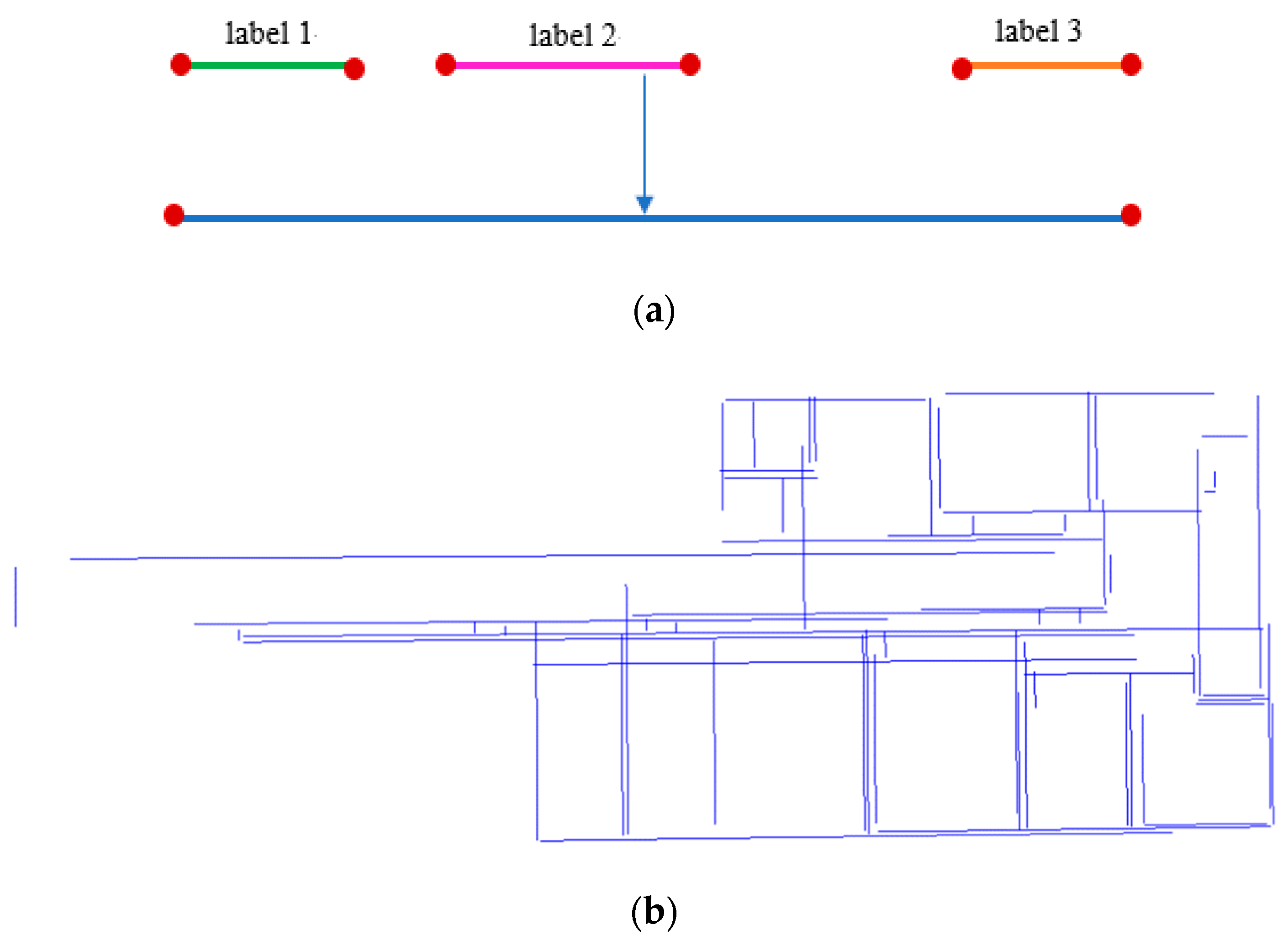
Lastly, the main lines consist of line groups. A mainline is determined at least by a starting point, an endpoint, an offset, and a normal vector. The normal vector of the seed line and the mean offset serve as the final parameters for the mainline. The line groups with different labels are then projected onto the mainline to find the endpoints and create the bounding boxes (see Figure 9a). The final main lines are presented in Figure 9b.
3.3. Structured Model Reconstruction
3.3.1. Model Reconstruction
Figure 9b shows the line segments are incomplete due to missing point clouds. The lines are extended to form the enclosed floorplans (shown in green lines in Figure 10). Lines in the enclosed floorplans have topology and the point clouds in the segmented rooms have semantic information. Thus, the line segments and point clouds with individual rooms are can be used as constraint conditions in building the two-dimensional floorplan using multi-label graph cuts. The labelled Point clouds are projected on the 2D polygon floorplan is shown in Figure 10. Each cell is assigned a label from set , which includes one label for each room plus an additional label for the outer space. Each line cell is assigned a label from the initial . The labelled line segments are used to segregate cells from adjacent region, of which cell labels should be different. Our approach differs from Ochmann’s work [15,22] such that the line segments are projected directly on the floorplan and divided into 2D line cells to improve the accuracy and efficiency of the model. With the approach expressed as an energy minimization function [31], the 2D polygons and lines are globally optimized to build the floorplan model, which are then extended to the estimated the floor and ceiling heights from segmented surfaces to build 3D room models. Figure 11 shows that the reconstructed model can better retain the details of indoor scene.
3.3.2. Room Structured Connection
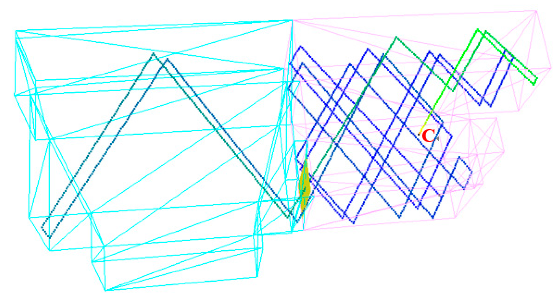
The above reconstructed models are expressing room semantic and geometric information, but still lacks room topological connection types. In the last step, the room’s structural connection is recreated. For indoor scenes, the space created by a door is a type of connection space. Thus, the door’s position is used to analyze the room connection types. In this study, the doors were extracted based on the segmented surfaces, and the model reconstruction is based on the horizontal slice of the segmented rooms. To correct some distance errors introduced during reconstruction, the detected door are attached to the walls if the following conditions must be satisfied: (a) the door must be parallel to a wall; (b) the distance along the normal should be less than the threshold of 0.2 m; and, (c) the door completely overlaps with the walls. The door connecting adjacent rooms is a subspace with thickness. Figure 12 shows the structured model with the reconstituted doors.
Every room is associated with geometry elements that ceiling, floor, walls, doors and windows. In our work, openings between neighboring rooms are detected to obtain a room connectivity graph, in addition, for each wall of the room, we search a matching, approximately parallel surface with opposing normal orientation within user-defined distance and angle thresholds. Each matching pair of wall surfaces forms adjacent rooms. According to these rules, a building’s room topology graph is constructed. If a space that is connected to more than three rooms and has many doors that is labeled a corridor. The rooms with topological relationship are shown in Figure 13, which can be applied to a service application in an indoor environment.
3.3.3. G Signal Intensity Simulation
In the 5G era, 5G devices have design features that support higher signal frequency and the shorter wavelength to generate faster transmission speed; however, this leads to diminished capability of penetrating through walls [48]. With 80% of today’s businesses occurring indoors, setting up large-scale small base stations to increase signal intensity has become a common occurrence. However, due to the complexities of the indoor environment (e.g., occlusion problems), network construction has become a challenging undertaking.
In this study, the output structured models have three properties: semantic, geometric, and connection types. These models are made up of basic building elements, such as the ceilings, floors, walls, windows, doors and pillars, which have direct effect on signal propagation in the real world. Thus, the structured model can become an important tool in analyzing 5G signal simulation.
According to the standard of 3GPP [49], the non-line-of-sight signal propagation loss model of indoor space is expressed:
where is the propagation loss; is the max propagation distance ; and, is frequency of the electromagnetic wave . The formula suggests that greater propagation loss occurs with larger wave frequency or with longer propagation distance. In an ideal indoor environment (no attenuation losses), when the frequency remains constant, the propagation loss increases with increasing distance, which then decreases the power received by the receiver.
The indoor environment is comprised of open cubicles, walled offices, open areas, corridors, etc. In this study, the 5G base stations were assumed to be located at the height of 2 m, near the ceilings. The ray-tracing solution is adopted to provide a detailed multipath and accurately simulate the spatial variation. Figure 14 illustrates the principle of single signal propagation, where the intensity multipath results from the reflection of walls and transmission of openings.
In our experiment, the signal propagation intensity was simulated in the structured model. Three base stations were mounted at the corridor and a room, as shown in Figure 15a. Every base station was assumed to be at the center of a sphere, randomly launching 150 rays. Using a frequency of 100 GHz, the intensity was calculated within a range of 100 m using the signal propagation loss model (see Figure 15b). The profile provided an effective means of measuring the changes of signal intensity and became a useful tool in visualization and inspection of 3D interpolation results. Therefore, the interpolation method of Inverse Distance Weight method (IDW) used in simulating the intensity profile can be calculated with:
where the intensity value of the interpolation point is defined as the weighted average value of known point intensity value ; is the Euclidean distance from interpolation point to its nearest sampling point; and, is the power exponent. Finally, the profile result is shown in Figure 15c.
4. Experiment
4.1. Datasets
The proposed method was tested on four datasets acquired by MLS in different indoor scenes, as shown in Figure 16. Table 1 lists the technical specifications of system, and the Table 2 details the specifications of the point clouds. The first dataset, the ISPRS Benchmark Data [50], was captured using a handheld scanner, Zeb-Revo, in one of the buildings at the Technical University of Braunschweig, Germany. The data were acquired from across two floors connected via a staircase. The point clouds and trajectories are shown in Figure 16a. The walls had different thicknesses, the ceilings were of different heights, and the level of point cloud quality was high. The second dataset was captured in the 14th floor of the Technology Building of Shenzhen University, using our own developed backpack laser scanning (BLS), which contains a 16-beam 3D laser scanner. The location was in a corridor with glass walls and contains a number of moving objects; the collected point clouds had a high level of noise, as shown in Figure 16b. The third and fourth datasets were acquired on a corridor and a parking lot by the backpack mapping system of Xiamen University (shown in Figure 16c,d). This laser scanning system [37] contains two 16-beam laser scanners and can obtain higher quality 3D point cloud data.
4.2. Parameters
The parameters of the proposed indoor structural model method for four datasets are listed in Table 3. Based on preliminary findings from the experiments, proposed methods showed robustness, and most of the parameters were insensitive to point cloud data in various indoor scenes and did not require manual modification. For opening extraction, the point clouds were transform into 2D image, where is the pixel size, and are the width and height of the regularized door; and, and are the width and height of the regularized window. For room segmentation, the point clouds were transformed into 3D grids, where is the size of 3D grid; and, are weight parameters used for balancing importance between data term and smooth term in the energy function. For the line global optimization, the and were used to correct the angle and distance value of line; is the nearest neighbor number of every line; and, is weight parameter used for balancing different terms in the energy function. For clustering similar lines, and were the angle and distance threshold. In 5G signal intensity simulation, is the signal propagation distance, is the frequency of the electromagnetic wave, and is the power exponent by IDW interpolation method. These parameters can be depended on the point cloud data from different indoor scenes with similar characteristics.
4.3. Results
The algorithm was implemented in C++, edited by Microsoft Visual Studio 2017. All experiments were performed with a Window 10, 64-bit operating system with an Alienware Intel (R) Core (TM) i7-7700HQ CPU @ 2.80 GHz and a 16GB RAM.
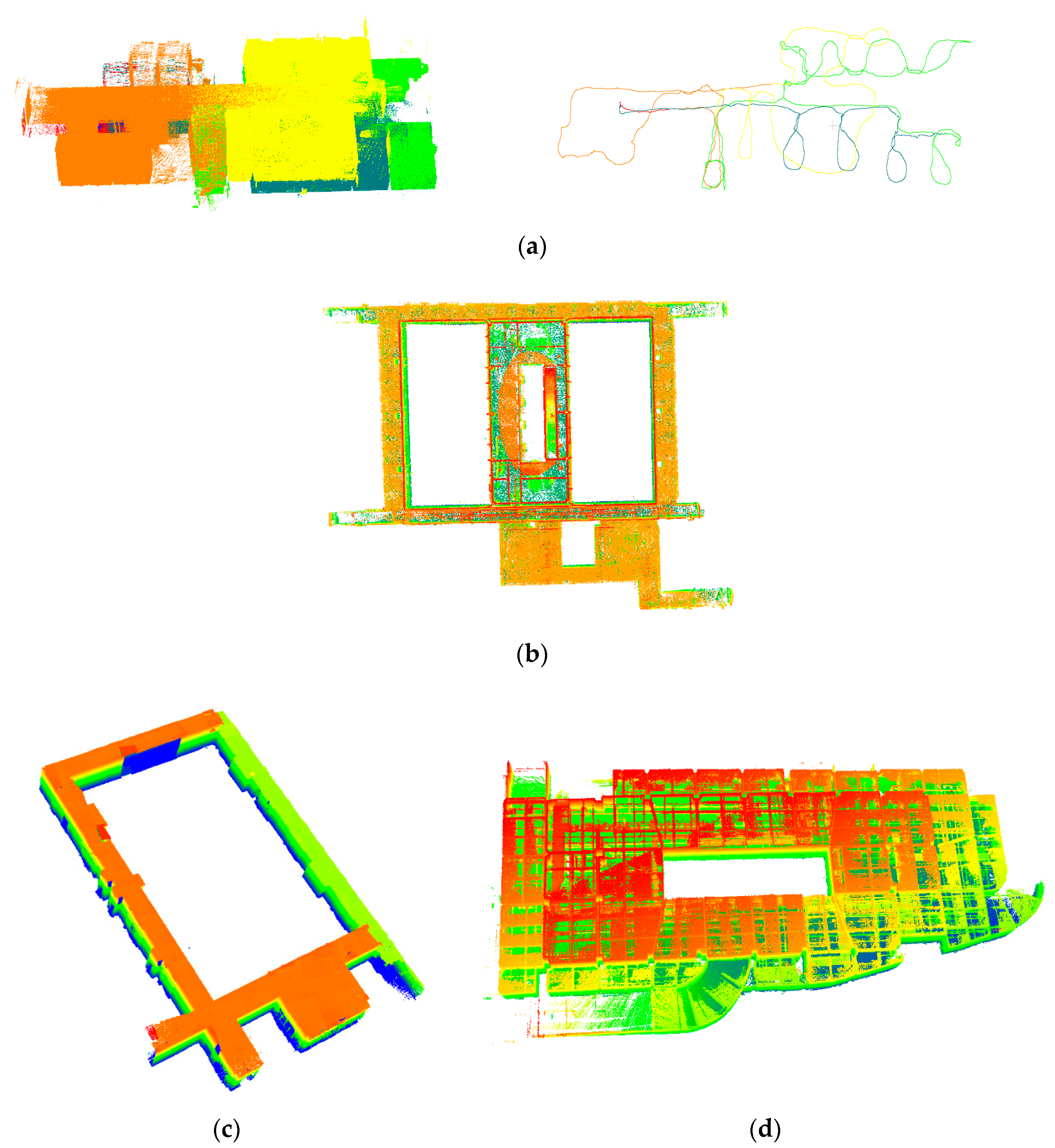
Preliminary visual results of the structured model showed correctness and completeness of the model. For the benchmark data (shown in Figure 17a), the width and length of the extracted doors (green) and windows (yellow) were close to the true value. The room segmentation results of the first and second floors (as shown in Figure 17b) showed that the unstructured point clouds were correctly partitioned based on the multi-label graph cuts. In order to ensure the model accuracy, the structural model was reconstructed using visible point clouds, which eliminated the error from wall thickness estimation. Figure 17c,d show the reconstructed models to have detailed wall information. The doors (yellow) and windows (red) were correctly positioned and completely embedded within the walls, and the adjacent rooms had different heights. The structured model and original point clouds were well-matched, as shown in Figure 17e.
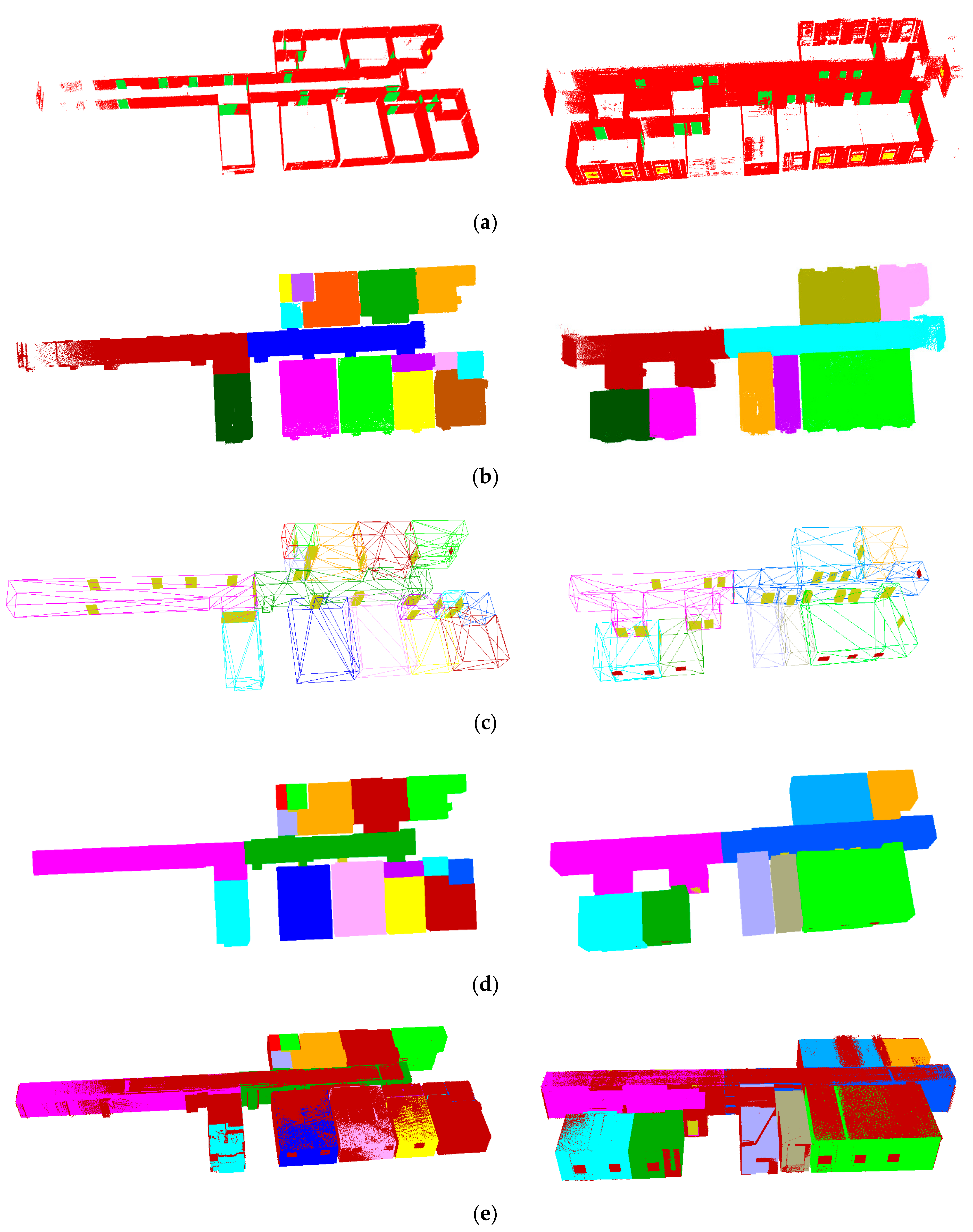
For the corridor data of Shenzhen University, the acquired point clouds suffered from multiple reflections and refraction due to the glass walls, which resulted in the dramatic challenges during model reconstruction. Figure 18a shows the structured models, while Figure 18b shows that the detailed vector models of walls, pillars, the doors (green). The closed-loop polyhedron was created using the constrained Delaunay triangulation [51], which the detected closed polygons are as boundary rings. Figure 18c,d illustrate that the reconstructed models and point clouds are well matched. For the Xiamen University corridor, a high accuracy indoor structured model was obtained. Figure 19a,b show the structural models and the wall models, which are presented with detailed regularization information and accurate room representation with uneven ceiling heights. The doors (green) and windows (red) were correctly detected and completely embedded within the walls. The point clouds and the reconstructed model are well-matched, as presented in Figure 19c,d.
For the parking lot in Xiamen University, the point clouds showed an excessively high level of noise. However, our proposed framework is still well-built even with incomplete data caused by severe occlusion (see Figure 20a,b). Our approach can auto-complete and generate closed-loop polyhedrons, and also correctly reconstruct the slant ceiling, floor, vertical walls, and regularized pillars. However, some curved walls are represented by many small polygons. The reconstructed models matched well with the original point clouds, as shown in Figure 20c,d.
More details of the results are displayed in Figure 21, despite the presence of noises and incomplete in the point clouds, our reconstructed models are of high correctness and well fit to the original point clouds.
For 5G signal intensity simulation, we tested our method on the structural model reconstructed from the benchmark data, as shown in Figure 22. The signal intensity is shown to drastically decrease from the base stations when three were mounted on the first floor, as illustrated by the changing colors of intensity (red to blue) in Figure 22a. In order to visualize the trend of signal intensity loss, a horizontal intensity profile was generated using the IDW interpolation method and is shown in Figure 22b. Similarly, the results from the multipath signal propagation and horizontal profile from the second floor are shown in Figure 22c,d. In Figure 22e, the received energy value is shown to significantly decrease with increasing distance under the path loss model.
5. Evaluation and Discussion
Four real-world datasets captured using MLS were used to test our proposed methodology. Field experiments were used to analyze the visualization results and correctness of the semantic information and the spatial and topological relations of reconstructed models, as shown in Figure 17, Figure 18, Figure 19, Figure 20 and Figure 21. The quantitative evaluation of the model included basic element extraction, running time, and geometric errors, as shown in Table 4, Table 5 and Table 6 and Figure 23.
5.1. Quantitative Evaluation
Table 4 and Table 5 enumerate key properties of the reconstructed model, including the number of points, actual and extracted basic elements, and runtime. For the statistical analysis of geometric errors, the reconstructed results with real data did not contain ground-truth data, so we used the distance from each original point cloud to its corresponding model plane as geometric error. The summary is presented in Table 6 and Figure 23.
In Table 4, for the benchmark data, 42 doors and 8 windows were correctly detected: 20 doors and 1 window on the first floor and 22 doors and 7 windows on the second floor. The closed doors cannot be detected. The detection failure for the other windows was due to high sparsity and noise in the wall point clouds. However, all rooms and corridors were correctly segmented and had no under-segmentation or over-segmentation. The Shenzhen corridor dataset had high levels of noise and sparsity due to multiple reflections of moving objects and refraction from the glass wall. However, the structured information of pillars and doors were accurately extracted. For the Xiamen corridor dataset with high-quality point clouds, all openings were correctly detected. For the Xiamen parking lot dataset, 18 pillars were correctly detected. In terms of time efficiency, the reconstruction of the four real-world datasets required little runtime (see Table 5), with only the room segmentation taking relatively more processing time. The results indicate our proposed methodology has high modelling efficiency with wide-ranging applications in different indoor scenes.
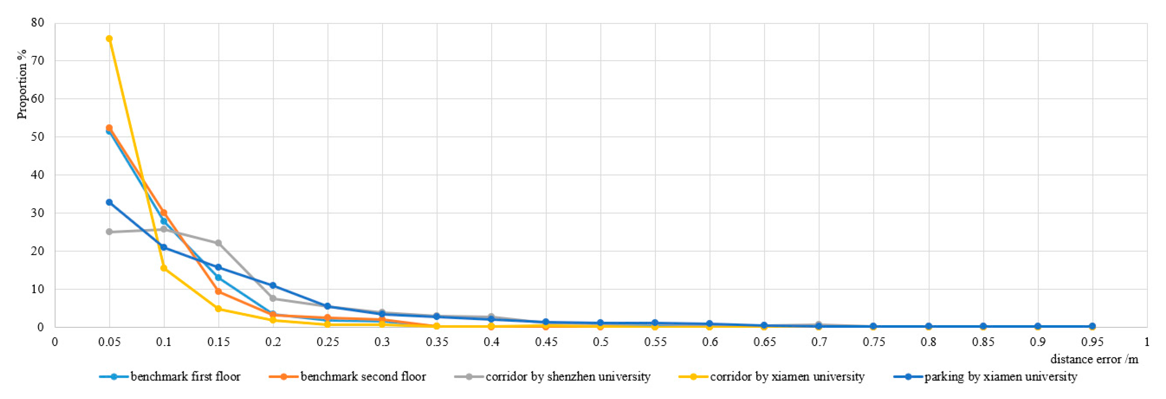
The summary of Euclidean distance deviation and diagram are shown in Table 6 and Figure 23. The reconstruction accuracy from the Xiamen corridor was highest, having 75.83% of point distance deviation within the 0.05 m range. The two floors from the benchmark showed comparable results with 51.50% (1st floor) and 52.31% (2nd floor) of deviations coming from the 0.05 m range. For the Shenzhen Corridor and Xiamen parking lot, the percentage of deviation within 0.05 m reached 25.10% and 32.82% respectively. This indicates that when using our approach, the reconstruction quality is heavily dependent on the quality of point clouds. Nevertheless, our method shows it can provide reliable and accurate reconstruction of indoor scenes within the 0.10 m range without the need for manual intervention.
5.2. Limitations
A major technical limitation of our method is that the detection of openings are highly dependent on the geometric quality of point clouds, which for indoor scenes with high amount of noise, could be very problematic. Also, the curved walls are represented with many small polygons, indicating that irregular structures could not be expressed as meshes. Then, the output results in this study are surface models; however, BIM standard models are often represented as volumetric building entities with walls, floors, ceilings, and topological information, thus, the surface models will lead to limit the expression of model thickness in practice. Lastly, in 5G signal simulation, the type of wall materials, which could create varying degrees of signal loss, was ignored for simplification, which results in some errors with actual situation.
6. Conclusions and Outlook
The current bottleneck in 3D indoor reconstruction is the low level of automation and accuracy in the reconstruction of the complex indoor environment. To address this problem, we proposed a novel method that combines the rich structures of lines and 3D geometric information of surfaces to automatically build a three-dimensional structured model from MLS point clouds. First, a fully automatic room segmentation is performed on the unstructured point clouds via multi-label graph cuts to overcome over-segmentation problems. The floorplan lines are then extracted and regularized from the image to obtain detail structural information. Finally, the segmented room, line, and surface elements are used as semantic information, and the 3D structured models are reconstructed by multi-label graph cuts. We showed how our proposed approach is able to accurately reconstruct real-world datasets without requiring manual operation. Also, the signal intensity simulation for 5G small base station was conducted using the results of our 3D model, which showed how our proposed technique can be very useful in such an application.
We tested our method on four real-world datasets acquired using the MLS. In analyzing the results, we included the assessment of the geometric elements, time-efficiency, and geometric errors in the evaluation. Experimental results show that the reconstructed structured models, including ceilings, floors, walls, doors, windows, and pillars, etc. The Combination of linear structures with 3D geometric surfaces to reconstruct structured models, which improve the computational efficiency and structural accuracy. The resulting models show that the geometric error of is within 0.1m for different indoor scenes. The detection of geometric elements is highly dependent on the geometric quality of point clouds. For our future endeavors, we will try to combine image and point clouds to further enrich the model results, which could help improve opening detection and compensate for poor point cloud quality. We will also reconstruct the full volumetric models using the extracted geometric elements, and further close to the requirements for Building Information Modeling. Finally, we will be investigating further the use of our approach in optimal location for 5G small base stations and other similar technologies, as well as considering other applications that may benefit from our approach.
Author Contributions
Conceptualization, Y.C., Q.L.; methodology, Y.C., Q.L. and Z.D.; software, Y.C. and Z.D.; validation, Y.C. and Q.L.; formal analysis, Y.C. and Z.D.; investigation, Y.C. and Z.D., resources, Q.L.; writing—original draft preparation, Y.C., Q.L. and Z.D.; writing—review and editing, Y.C., Q.L. and Z.D.; visualization, Y.C. and Z.D.; supervision, Q.L. and Z.D.; project administration, Q.L. and Z.D.
Funding
This research was funded by the Key Program of the National Natural Science Foundation of China (No. 41531177), the National Science Fund for Distinguished Young Scholars of China (No. 41725005), the Technical Cooperation Agreement between Wuhan University and Huawei Space Information Technology Innovation Laboratory (No. YBN2018095106), the National Natural Science Foundation of China (No. 41901403), the National Key Research and Development Program of China (No. 2016YFB0502203).
Acknowledgments
We would like to thank the ISPRS Commission WG IV/5 for provision of the data. In addition, we also thank to Key Laboratory of Sensing and Computing for Smart City and the School of Information Science and Engineering, Xiamen University for providing the corridor and parking lot datasets, and special thanks to the professional English editing service from EditX to improve the language.
Conflicts of Interest
The authors declare no conflict of interest.
References
- Becker, S.; Peter, M.; Fritsch, D. Grammar-Supported 3d Indoor Reconstruction from Point Clouds for As-Built Bim. ISPRS Int. Arch. Photogramm. Remote Sens. Spat. Inf. Sci. 2015, II-3/W4, 17–24. [Google Scholar] [CrossRef]
- Vilariño, L.D.; Boguslawski, P.; Khoshelham, K.; Lorenzo, H.; Mahdjoubi, L. Indoor Navigation from Point Clouds: 3d Modelling and Obstacle Detection. ISPRS Int. Arch. Photogramm. Remote Sens. Spatial Inf. Sci. 2016, XLI-B4, 275–281. [Google Scholar]
- Vilariño, L.D.; Frias, E.; Balado, J.; Gonzalezjorge, H. Scan planning and route optimization for control of execution of as-designed BIM. ISPRS Int. Arch. Photogramm. Remote Sens. Spatial Inf. Sci. 2018, XLII-4, 143–148. [Google Scholar]
- Boyes, G.; Ellul, C.; Irwin, D. Exploring bim for operational integrated asset management-a preliminary study utilising real-world infrastructure data. ISPRS Int. Arch. Photogramm. Remote Sens. Spatial Inf. Sci. 2017, IV-4/W5, 49–56. [Google Scholar] [CrossRef]
- Tomasi, R.; Sottile, F.; Pastrone, C.; Mozumdar, M.M.R.; Osello, A.; Lavagno, L. Leveraging bim interoperability for uwb-based wsn planning. IEEE Sens. J. 2015, 15, 5988–5996. [Google Scholar] [CrossRef]
- Rafiee, A.; Dias, E.; Fruijtier, S.; Rafiee, A.; Dias, E.; Fruijtier, S.; Scholten, H. From bim to geo-analysis: View coverage and shadow analysis by bim/gis integration. Procedia Environ. Sci. 2014, 22, 397–402. [Google Scholar] [CrossRef]
- Tang, D.; Kim, J. Simulation support for sustainable design of buildings. In Proceedings of the CTBUH International Conference, Shanghai, China, 16–19 September 2014. [Google Scholar]
- Boguslawski, P.; Mahdjoubi, L.; Zverovich, V.E.; Fadli, F. Two-graph building interior representation for emergency response applications. ISPRS Int. Arch. Photogramm. Remote Sens. Spatial Inf. Sci. 2016, III-2, 9–14. [Google Scholar]
- Bassier, M.; Vergauwen, M. Clustering of Wall Geometry from Unstructured Point Clouds Using Conditional Random Fields. Remote Sens. 2019, 11, 1586. [Google Scholar] [CrossRef]
- Ikehata, S.; Yang, H.; Furukawa, Y. Structured Indoor Modeling. In Proceedings of the IEEE International Conference on Computer Vision, Santiago, Chile, 7–13 December 2015. [Google Scholar]
- Wang, J.; Xu, K.; Liu, L.; Cao, J.; Liu, S.; Yu, Z.; Gu, X. Consolidation of low-quality point clouds from outdoor scenes. Comput. Graph. Forum. 2013, 32, 207–216. [Google Scholar] [CrossRef]
- Mura, C.; Mattausch, O.; Villanueva, A.J.; Gobbetti, E.; Pajarola, R. Automatic room detection and reconstruction in cluttered indoor environments with complex room layouts. Comput. Graph. 2014, 44, 20–32. [Google Scholar] [CrossRef] [Green Version]
- Ochmann, S.; Vock, R.; Wessel, R.; Tamke, M.; Klein, R. Automatic generation of structural building descriptions from 3D point cloud scans. In Proceedings of the International Conference on Computer Graphics Theory and Applications, Lisbon, Portugal, 5–8 January 2014. [Google Scholar]
- Turner, E.; Cheng, P.; Zakhor, A. Fast, Automated, Scalable Generation of Textured 3D Models of Indoor Environments. IEEE J. Sel. Top. Signal. Process. 2015, 9, 409–421. [Google Scholar] [CrossRef]
- Ochmann, S.; Vock, R.; Wessel, R.; Klein, R. Automatic reconstruction of parametric building models from indoor point clouds. Comput. Graph. 2016, 54, 94–103. [Google Scholar] [CrossRef] [Green Version]
- Ambrus, R.; Claici, S.; Wendt, A. Automatic Room Segmentation from Unstructured 3-D Data of Indoor Environments. In Proceedings of the International Conference on Robotics and Automation, Singapore, 29 May–3 June 2017. [Google Scholar]
- Wang, R.; Xie, L.; Chen, D. Modeling Indoor Spaces Using Decomposition and Reconstruction of Structural Elements. Photogramm. Eng. Remote Sens. 2017, 83, 827–841. [Google Scholar] [CrossRef]
- Vilariño, L.D.; Verbree, E.; Zlatanova, S.; Diakité, A. Indoor Modelling from Slam-Based Laser Scanner: Door Detection to Envelope Reconstruction. ISPRS Int. Arch. Photogramm. Remote Sens. 2017, XLII-2/W7, 345–352. [Google Scholar]
- Li, L.; Su, F.; Yang, F.; Zhu, H.; Li, D.; Zuo, X.; Li, F.; Liu, Y.; Ying, S. Reconstruction of Three—Dimensional (3D) Indoor Interiors with Multiple Floors via Comprehensive Segmentation. Remote Sens. 2018, 10, 1281. [Google Scholar] [CrossRef]
- Yang, F.; Li, L.; Su, F.; Li, D.L.; Zhu, H.H.; Ying, S.; Zuo, X.K.; Tang, L. Semantic decomposition and recognition of indoor spaces with structural constraints for 3D indoor modelling. Automat. Constrn. 2019, 106, 102913. [Google Scholar] [CrossRef]
- Stichting, C.; Centrum, M.; Dongen, S.V. A Cluster Algorithm for Graphs; CWI: Amsterdam, The Netherlands, 2000; pp. 1–40. [Google Scholar]
- Ochmann, S.; Vock, R.; Klein, R. Automatic reconstruction of fully volumetric 3D building models from oriented point clouds. ISPRS J. Photogramm. Remote Sens. 2019, 151, 251–262. [Google Scholar] [CrossRef] [Green Version]
- Sanchez, V.; Zakhor, A. Planar 3D modeling of building interiors from point cloud data. In Proceedings of the IEEE International Conference on Image Processing, Orlando, FL, USA, 30 September–3 October 2012. [Google Scholar]
- Lafarge, F.; Alliez, P. Surface Reconstruction through Point Set Structuring. Comput. Graph. Forum. 2013, 32, 225–234. [Google Scholar] [CrossRef] [Green Version]
- Monszpart, A.; Mellado, N.; Brostow, G.; Mitra, N. RAPter: Rebuilding man-made scenes with regular arrangements of planes. Acm Trans. Graph. 2015, 34, 103. [Google Scholar] [CrossRef]
- Awrangjeb, M.; Gilani, S.A.; Siddiqui, F.U. An Effective Data-Driven Method for 3-D Building Roof Reconstruction and Robust Change Detection. Remote Sens. 2018, 10, 1512. [Google Scholar] [CrossRef]
- Xiao, J.; Furukawa, Y. Reconstructing the world’s museums. In Proceedings of the European Conference on Computer Vision, Florence, Italy, 7–13 October 2012. [Google Scholar]
- Schnabel, R.; Wahl, R.; Klein, R. Efficient RANSAC for point-cloud shape detection. Comput. Graph. Forum 2007, 26, 214–226. [Google Scholar] [CrossRef]
- Mura, C.; Mattausch, O.; Pajarola, R. Piecewise-planar Reconstruction of Multi-room Interiors with Arbitrary Wall Arrangements. Comput. Graph. Forum 2016, 35, 179–188. [Google Scholar] [CrossRef]
- Boulch, A.; Gorce, M.D.L.; Marlet, R. Piecewise-Planar 3D Reconstruction with Edge and Corner Regularization. Comput. Graph. Forum. 2014, 33, 55–64. [Google Scholar] [CrossRef] [Green Version]
- Cui, Y.; Li, Q.; Yang, B.; Xiao, W.; Chen, C.; Dong, Z. Automatic 3-D Reconstruction of Indoor Environment with Mobile Laser Scanning Point Clouds. IEEE J. Sel. Top. Appl. Earth Observ. Remote Sens. 2019, 99, 1–14. [Google Scholar] [CrossRef]
- Lin, Y.; Wang, C.; Chen, B.L.; Zai, D.W.; Li, J. Facet Segmentation-Based Line Segment Extraction for Large-Scale Point Clouds. IEEE Trans. Geosci. Remote Sens. 2017, 55, 4839–4854. [Google Scholar] [CrossRef]
- Xia, S.; Wang, R. Façade Separation in Ground-Based LiDAR Point Clouds Based on Edges and Windows. IEEE J. Sel. Top. Appl. Earth Observ. Remote Sens. 2019, 12, 1041–1052. [Google Scholar] [CrossRef]
- Lu, X.; Liu, Y.; Li, K. Fast 3D Line Segment Detection from Unorganized Point Cloud. In Proceedings of the IEEE Conference on Computer Vision Pattern Recognition, Long Beach UA, CA, USA, 15–21 June 2019. [Google Scholar]
- Liu, C.; Wu, J.; Furukawa, Y. FloorNet: A Unified Framework for Floorplan Reconstruction from 3D Scans. In Proceedings of the European Conference on Computer Vision, Munich, Germany, 8–14 September 2018. [Google Scholar]
- Oesau, S.; Lafarge, F.; Alliez, P. Indoor scene reconstruction using feature sensitive primitive extraction and graph-cut. ISPRS J. Photogramm. Remote Sens. 2014, 90, 68–82. [Google Scholar] [CrossRef] [Green Version]
- Wang, C.; Hou, S.; Wen, C.; Gong, Z.; Li, Q.; Sun, X.; Li, J. Semantic line framework-based indoor building modeling using backpacked laser scanning point cloud. ISPRS J. Photogramm. Remote Sens. 2018, 143, 150–166. [Google Scholar] [CrossRef]
- Bauchet, J.; Lafarge, F. KIPPI: KInetic Polygonal Partitioning of Images. In Proceedings of the IEEE Conference on Computer Vision Pattern Recognition, Salt Lake City, UT, USA, 18–22 June 2018. [Google Scholar]
- Sui, W.; Wang, L.; Fan, B.; Xiao, H.; Wu, H.; Pan, C. Layer-Wise Floorplan Extraction for Automatic Urban Building Reconstruction. IEEE Trans. Vis. Comput. Graph. 2016, 22, 1261–1277. [Google Scholar] [CrossRef]
- Novakovic, G.; Lazar, A.; Kovacic, S.; Vulic, M. The Usability of Terrestrial 3D Laser Scanning Technology for Tunnel Clearance Analysis Application. Appl. Mech. Mater. 2014, 683, 219–224. [Google Scholar] [CrossRef]
- Suzuki, S.; Be, K. Topological structural analysis of digitized binary images by border following. Comput. Vis. Graph. Image Process. 1985, 30, 32–46. [Google Scholar] [CrossRef]
- OpenCV. Available online: https://opencv.org/ (accessed on 2 April 2019).
- Boykov, Y.; Kolmogorov, V. An experimental comparison of min-cut/max-flow algorithms for energy minimization in vision. IEEE Trans. Pattern Anal. Mach. Intell. 2004, 26, 1124–1137. [Google Scholar] [CrossRef] [PubMed]
- Boykov, Y.; Veksler, O.; Zabih, R. Fast approximate energy minimization via graph cuts. IEEE Trans. Pattern Anal. Mach. Intell. 2001, 23, 1222–1239. [Google Scholar] [CrossRef]
- Kolmogorov, V.; Zabin, R. What energy functions can be minimized via graphcuts? IEEE Trans. Pattern Anal. Mach. Intell. 2002, 26, 147–159. [Google Scholar] [CrossRef] [PubMed]
- Von Gioi, R.G.V.; Jakubowicz, J.; Morel, J.M.; Randall, G. LSD: A Fast Line Segment Detector with a False Detection Control. IEEE Trans. Pattern Anal. Mach. Intell. 2010, 32, 722–732. [Google Scholar] [CrossRef] [PubMed]
- Kümmerle, R.; Grisetti, G.; Strasdat, H.; Konolige, K.; Burgard, W. G 2 o: A general framework for graph Optimization. In Proceedings of the IEEE International Conference on Robotics and Automation, Shanghai, China, 9–13 May 2011. [Google Scholar]
- Yang, G.; Chen, J. Research on Propagation Model for 5G Mobile Communication Systems. Mob. Commun. 2018, 42, 28–33. [Google Scholar]
- 5G. Study on Channel Model for Frequencies from 0.5 to 100 GHZ (3GPP TR 38.901 version 14.0.0 release 14). Available online: http://www.etsi.org/standards-search (accessed on 5 May 2017).
- Khoshelham, K.; Vilariño, L.D.; Peter, M.; Kang, Z.; Acharya, D. The ISPRS benchmark on indoor modelling. Int. Arch. Photogramme. Remote Sens. Spat. Inf. Sci. 2017, XLII-2/W7, 367–372. [Google Scholar] [CrossRef]
- Chew, L.P. Constrained Delaunay triangulations. Algorithmica 1989, 4, 97–108. [Google Scholar] [CrossRef]
Figure 1.
Flowchart of the proposed method.

Figure 2.
Detection of openings. (a) Extracted wall surfaces. (b) Wall surfaces converted into binary image. (c) Template match. (d) Detected doors.
Figure 2.
Detection of openings. (a) Extracted wall surfaces. (b) Wall surfaces converted into binary image. (c) Template match. (d) Detected doors.

Figure 3.
The diagram of visible point clouds of simulated trajectory points. (a) Original point clouds. (b) Original point clouds divided into uniform grids. (c) Sample trajectory points. (d) Visibility analysis based on line-of-sight.
Figure 3.
The diagram of visible point clouds of simulated trajectory points. (a) Original point clouds. (b) Original point clouds divided into uniform grids. (c) Sample trajectory points. (d) Visibility analysis based on line-of-sight.

Figure 4.
Simulating visible point clouds of sample trajectories. (a) The visible points of the three trajectory points 26, 30, and 33. (b) Visible points limited by door.
Figure 4.
Simulating visible point clouds of sample trajectories. (a) The visible points of the three trajectory points 26, 30, and 33. (b) Visible points limited by door.

Figure 5.
Position of doors subdivide trajectory segments. (a) Sample trajectory points. (b) Partition of trajectory segments.
Figure 5.
Position of doors subdivide trajectory segments. (a) Sample trajectory points. (b) Partition of trajectory segments.

Figure 6.
Point clouds before and after space labeling. (a) Original point clouds. (b) Point clouds after space labeling.
Figure 6.
Point clouds before and after space labeling. (a) Original point clouds. (b) Point clouds after space labeling.

Figure 7.
Floorplan Line extraction. (a) Split labeled point clouds from given height. (b) The conversion of projected points into a binary image. (c) Extraction of line elements with label information.
Figure 7.
Floorplan Line extraction. (a) Split labeled point clouds from given height. (b) The conversion of projected points into a binary image. (c) Extraction of line elements with label information.

Figure 8.
Global optimization of lines. (a) Correction of angle. (b) Correction of distance. (c) The global optimization results.
Figure 8.
Global optimization of lines. (a) Correction of angle. (b) Correction of distance. (c) The global optimization results.

Figure 9.
Clustering similar lines. (a) The line groups project onto the cluster line. (b) The final main lines.
Figure 9.
Clustering similar lines. (a) The line groups project onto the cluster line. (b) The final main lines.

Figure 10.
Line segments and point clouds as constraint conditions.

Figure 11.
The reconstructed room models.

Figure 12.
The structured model with openings.

Figure 13.
The rooms with topological relationship (the solid lines are connected by the doors, and the dotted lines are the connected by adjacent walls).
Figure 13.
The rooms with topological relationship (the solid lines are connected by the doors, and the dotted lines are the connected by adjacent walls).

Figure 14.
Principle of signal propagation (the signal intensity changes from strong to weak that corresponds to color from red to blue).
Figure 14.
Principle of signal propagation (the signal intensity changes from strong to weak that corresponds to color from red to blue).

Figure 15.
Signal intensity simulation. (a) Setting three base stations. (b) Multipath signal propagation. (c) Horizontal profile of signal intensity.
Figure 15.
Signal intensity simulation. (a) Setting three base stations. (b) Multipath signal propagation. (c) Horizontal profile of signal intensity.

Figure 16.
The experiment data. (a) Benchmark point clouds and trajectories acquired by handheld laser scanning (HLS), ZEB-REVO. (b) Point clouds acquired by Shenzhen University (BLS) system of Shenzhen University. (c) A closed-loop corridor by BLS system of Xiamen University. (d) Parking lot by BLS system of Xiamen University.

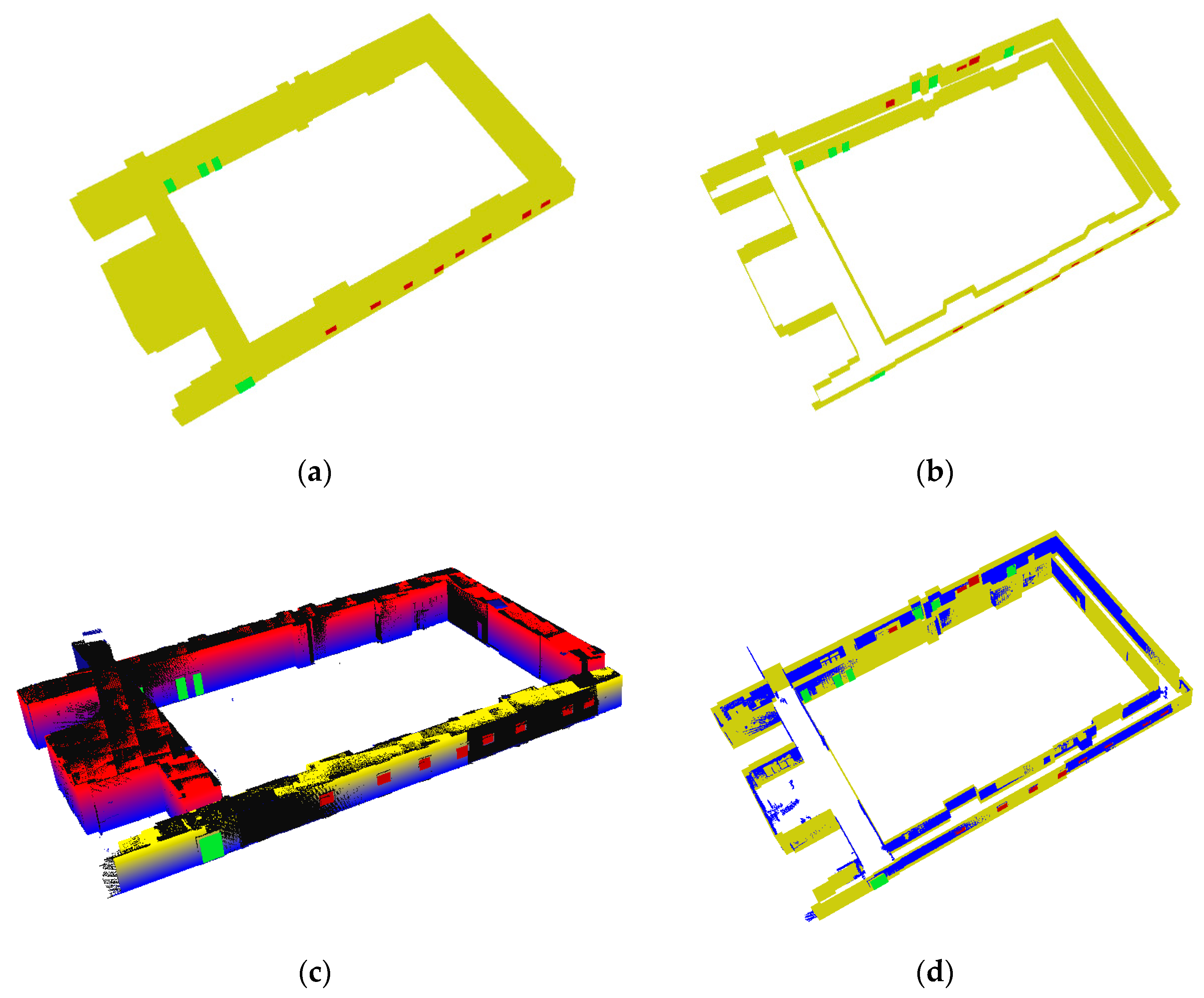
Figure 17.
Opening extraction, room segmentation, structural model and wireframe model results with the benchmark point clouds. (a) Doors (green) and windows (yellow) of the first and the second floors. (b) Segmented rooms of the first and second floors. (c) The structural models with doors and windows of the first and the second floors. (d) The wireframe models with doors and windows of the first and second floors. (e) Matching between the point clouds and the structured models on the first and second floors.

Figure 18.
Structural model results of the corridor at the Shenzhen University. (a) The structural model. (b) Vector model of walls and pillars. (c) Matching between point clouds and the structural model. (d) Matching between point clouds and vector model of walls and pillars.
Figure 18.
Structural model results of the corridor at the Shenzhen University. (a) The structural model. (b) Vector model of walls and pillars. (c) Matching between point clouds and the structural model. (d) Matching between point clouds and vector model of walls and pillars.

Figure 19.
Structural model results of the corridor at the Xiamen University. (a) The structural model. (b) Vector model of walls. (c) Matching between point clouds and structured model. (d) Matching between.
Figure 19.
Structural model results of the corridor at the Xiamen University. (a) The structural model. (b) Vector model of walls. (c) Matching between point clouds and structured model. (d) Matching between.

Figure 20.
Structural model results of the parking lot at the Xiamen university (a) The structural model with slant floor and ceiling. (b) Vector model of walls and pillars. (c) Matching between point clouds and structured model. (d) Matching between point clouds and the vector model of walls and pillars.

Figure 21.
Close-up views of selected details. (a) Benchmark point clouds and reconstructed model. (b) The point clouds and reconstructed model of the corridor at the Shenzhen University. (c) The point clouds and reconstructed model of the corridor at Xiamen University. (d) The point clouds and reconstructed model of the parking lot at Xiamen University.

Figure 22.
5G signal intensity simulation based on the structural model by benchmark data. (a) The multipath signal propagation on the first floor. (b) Horizontal profile of signal intensity on the first floor. (c) The multipath signal propagation on the second floor. (d) Horizontal profile of signal intensity on the second floor. (e) Received energy value.

Figure 23.
Euclidean distance deviation distribution map.


Table 1.
Technical specifications of the laser scanning system.
| Sensor | ZEB REVO | BLS (Shenzhen University) | BLS (Xiamen University) |
|---|---|---|---|
| Max range | 30 m | 100 m | 100 m |
| Speed (points/sec) | 43 × 103 | 300 × 103 | 300 × 103 |
| Horizontal Angular Resolution | 0.625° | 0.1–0.4° | 0.1–0.4° |
| Vertical Angular Resolution | 1.8° | 2.0° | 2.0° |
| Angular FOV | 270 × 360° | 30 × 360° | 2 × 30 × 360° |
Table 2.
Specifications of point clouds.
| Dataset | Benchmark Data | Corridor (Shenzhen University) | Corridor (Xiamen University) | Parking lot (Xiamen University) |
|---|---|---|---|---|
| Number of points | 21.560.263 | 1.980.911 | 2.098.634 | 7.683.766 |
| Clutter | Low | High | Low | High |
Table 3.
Parameters of the proposed indoor structural model method.
| Parameters | Values | Descriptions |
|---|---|---|
| Extracting Openings | ||
| The size of the pixel (point clouds transform into image) | ||
| The width and height of regularized door | ||
| The width and height of the regularized window | ||
| Segmentation of Rooms | ||
| The size of the 3D grid (point clouds transform into 3D grid) | ||
| Parameters of data term and smooth term of the energy function | ||
| Line Global Optimization | ||
| Angle correction of lines | ||
| Distance correction of lines | ||
| k-nearest of lines | ||
| The weight parameter of line global optimization | ||
| Cluster Similar Lines | ||
| Angle threshold of merging similar lines | ||
| Distance threshold of merging similar lines | ||
| 5G Signal Intensity Simulation | ||
| The signal propagation distance | ||
| The frequency of the electromagnetic wave | ||
| The power exponent by IDW interpolation | ||
Table 4.
Results of basic element extraction.
| Description | Number of Points | Actual/Detected Doors | Actual/Detected Windows | Actual/Detected Rooms | Actual/Detected Pillars |
|---|---|---|---|---|---|
| Benchmark data | 11,628,186 | 51/42 | 21/8 | 25/25 | 0/0 |
| Corridor (Shenzhen University) | 1,980,911 | 4/4 | 0/0 | 1/1 | 6/6 |
| Corridor (Xiamen University) | 7,683,766 | 8/8 | 11/11 | 1/1 | 0/0 |
| Parking Lot (Xiamen University) | 2,098,634 | 0/0 | 0/0 | 1/1 | 23/18 |
Table 5.
Running time for different scenes.
| Description | Surface Extraction (s) | Opening Detection (s) | Room Segmentation (s) | Line Regularization and Model Reconstruction (s) | Total Time (s) |
|---|---|---|---|---|---|
| Benchmark data | 80 | 19 | 287 | 49 | 435 |
| Corridor (Shenzhen University) | 9 | 4 | 0 | 24 | 37 |
| Corridor (Xiamen University) | 7 | 6 | 0 | 20 | 33 |
| Parking Lot (Xiamen University) | 28 | 0 | 0 | 32 | 60 |
Table 6.
Euclidean distance deviation for different scenes.
| Error/m | 0.05 | 0.10 | 0.15 | 0.20 | 0.25 | 0.30 | 0.35 | 0.40 | 0.45 | 0.50 | 0.55 | 0.60 | 0.65 | 0.70 | 0.75 | 0.80 | 0.85 | 0.90 | 0.95 |
| Benchmark first floor (%) | 51.50 | 27.68 | 12.92 | 3.26 | 1.73 | 1.61 | 0.28 | 0.21 | 0.20 | 0.11 | 0.10 | 0.09 | 0.07 | 0.07 | 0.08 | 0.05 | 0.02 | 0.01 | 0.01 |
| Benchmark second floor (%) | 52.31 | 30.09 | 9.36 | 3.20 | 2.41 | 2.11 | 0.31 | 0.07 | 0.01 | 0.02 | 0.02 | 0.01 | 0.01 | 0.02 | 0.01 | 0.01 | 0.01 | 0.01 | 0.01 |
| Corridor, Shenzhen University (%) | 25.10 | 25.81 | 22.02 | 7.45 | 5.51 | 3.81 | 3.02 | 2.55 | 1.10 | 0.81 | 0.82 | 0.40 | 0.51 | 0.50 | 0.14 | 0.12 | 0.21 | 0.01 | 0.11 |
| Corridor, Xiamen University (%) | 75.83 | 15.49 | 4.81 | 1.75 | 0.62 | 0.60 | 0.11 | 0.11 | 0.41 | 0.10 | 0.02 | 0.01 | 0.02 | 0.05 | 0.02 | 0.02 | 0.01 | 0.01 | 0.01 |
| Parking lot, Xiamen University (%) | 32.82 | 20.87 | 15.71 | 10.92 | 5.38 | 3.30 | 2.62 | 2.01 | 1.37 | 1.23 | 1.06 | 0.91 | 0.44 | 0.26 | 0.27 | 0.23 | 0.20 | 0.25 | 0.15 |
© 2019 by the authors. Licensee MDPI, Basel, Switzerland. This article is an open access article distributed under the terms and conditions of the Creative Commons Attribution (CC BY) license (http://creativecommons.org/licenses/by/4.0/).
Share and Cite
MDPI and ACS Style
Cui, Y.; Li, Q.; Dong, Z. Structural 3D Reconstruction of Indoor Space for 5G Signal Simulation with Mobile Laser Scanning Point Clouds. Remote Sens. 2019, 11, 2262. https://0-doi-org.brum.beds.ac.uk/10.3390/rs11192262
AMA Style
Cui Y, Li Q, Dong Z. Structural 3D Reconstruction of Indoor Space for 5G Signal Simulation with Mobile Laser Scanning Point Clouds. Remote Sensing. 2019; 11(19):2262. https://0-doi-org.brum.beds.ac.uk/10.3390/rs11192262
Chicago/Turabian StyleCui, Yang, Qingquan Li, and Zhen Dong. 2019. "Structural 3D Reconstruction of Indoor Space for 5G Signal Simulation with Mobile Laser Scanning Point Clouds" Remote Sensing 11, no. 19: 2262. https://0-doi-org.brum.beds.ac.uk/10.3390/rs11192262
Note that from the first issue of 2016, this journal uses article numbers instead of page numbers. See further details here.