Leafing Patterns and Drivers across Seasonally Dry Tropical Communities

Abstract

Investigating the timing of key phenological events across environments with variable seasonality is crucial to understand the drivers of ecosystem dynamics. Leaf production in the tropics is mainly constrained by water and light availability. Identifying the factors regulating leaf phenology patterns allows efficiently forecasting of climate change impacts. We conducted a novel phenological monitoring study across four Neotropical vegetation sites using leaf phenology time series obtained from digital repeated photographs (phenocameras). Seasonality differed among sites, from very seasonally dry climate in the caatinga dry scrubland with an eight-month long dry season to the less restrictive Cerrado vegetation with a six-month dry season. To unravel the main drivers of leaf phenology and understand how they influence seasonal dynamics (represented by the green color channel (Gcc) vegetation index), we applied Generalized Additive Mixed Models (GAMMs) to estimate the growing seasons, using water deficit and day length as covariates. Our results indicated that plant-water relationships are more important in the caatinga, while light (measured as day-length) was more relevant in explaining leafing patterns in Cerrado communities. Leafing behaviors and predictor-response relationships (distinct smooth functions) were more variable at the less seasonal Cerrado sites, suggesting that different life-forms (grasses, herbs, shrubs, and trees) are capable of overcoming drought through specific phenological strategies and associated functional traits, such as deep root systems in trees.

1. Introduction

Temporal patterns of leaf replacement, or leaf exchange phenology, are of major importance in understanding ecosystem processes such as carbon, water, and energy exchanges, controlling seasonal cycles of photosynthetic activity [1,2,3]. A high heterogeneity of leafing patterns has been observed for the tropics, as climate seasonality varies widely in the intensity and length of the dry season [1,4]. Identifying the main factors that regulate leaf phenology in the tropics is thus crucial to understand ecosystem dynamics and to efficiently forecast climate change impacts on these increasingly threatened environments.

Water and light availability are considered the main abiotic cues regulating the timing and periodicity of leaf production in tropical vegetations [4,5,6,7,8,9]. For instance, water availability regulates the length of the growing season and the phenological synchrony among cerrado species [4]. Seasonal communities with longer dry seasons exhibit limited photosynthetic activity and a marked annual periodicity of leaf flushing and senescence patterns, favoring a larger proportion of deciduous species [1,10,11,12]. In fact, within seasonally dry tropical forests, nearly all plant individuals lose leaves in a synchronic deciduous behavior during the dry season [1,13,14,15]. In areas with less pronounced dry seasons and elevated total annual rainfall, species and individuals may display different degrees of deciduousness, establishing communities with a wide range of leafing behaviors that may change according to soil moisture conditions, topography [8,16], and the intensity of the dry season ([4] and references therein).

In the tropics, variation in day-length, and consequently in available light, has major impacts towards higher latitudes, triggering the input of new leaves [6,7,8]. In tropical seasonal environments such as semi-deciduous forests and savannas day-length triggers early leaf flushing, anticipating the onset of the rainy season [4,8,17,18,19]. Plant lifeforms also have direct implications in determining species adaptations to water and light availability, and thereby on leafing phenology [19,20,21]. Trees can produce new leaves during the dry season due to their capacity to reach accumulated groundwater sources (deeper rooting systems), allowing plant growth when photosynthetically active radiation is at its maximum [4,20,22,23]. Contrarily, given their shallow root system and architectural constraints, grasses are highly dependent on precipitation and rapidly respond to rainfall events [20,24].

Large scale studies (e.g., [12,25]) have contributed to the understanding of ecosystem productivity constraints worldwide and land surface phenology has been an important tool to determine seasonality of leaf reflectance. Nonetheless, these studies consider general vegetation cover types at broader spatial scales and use summarized data sets (monthly temporal scales) and often overlook the need for ground validation and the pursue of processes and mechanisms underlying phenology at finer spatial and temporal scales [26,27].

Long-term phenological time series in the tropics are scarce, stimulating the search for reliable plant monitoring methods [28,29]. Imagery based on digital cameras, or “phenocams” has been considered an alternative method to successfully and continuously monitor plant greening across landscapes [30,31]. Phenocams can track temporal changes in leafing patterns across tropical seasonal environments [32,33], while reducing human labor, increasing accuracy by eliminating observer subjectivity, improving temporal resolution to an hourly/daily basis, and improved spatial resolution, which allow simultaneous multiple-sites monitoring [30,33,34,35].

Here, we conducted a novel phenological multi-site near-surface monitoring study using digital cameras to describe community leafing patterns in four Neotropical seasonally dry environments that differ in their degree of seasonality and vegetation structure: a seasonally dry tropical forest (SDTF), locally known as caatinga, and three different Cerrado (Neotropical savanna) vegetation types—two woody savannas (cerrado and dense cerrado) and a grassy shrubland savanna (cerrado shrubland). We combined time series of leaf phenology obtained by phenocams and local environmental variables observed at a fine temporal scales (daily) to describe the patterns of leaf flushing and senescence and to evaluate the constraints imposed by water, light, and temperature in all four vegetation types. Specifically, we investigated: (i) whether the timing and length of the growing season differs across the four seasonally dry tropical communities and what are the drivers of phenological transitions in each environment; and (ii) whether the growing season varies according to the vegetation structure (woody versus grassy) and degree of seasonality, determined by the water deficit observed during the dry season. We expected the growing season to differ between Cerrado and caatinga sites, with the leafing season responding to rainfall events in the caatinga, while Cerrado communities should be influenced by daylength (light availability) due to the milder and shorter dry season. We also expected leafing patterns of Cerrado communities to differ between woody and grassy vegetation types according to the temporal niche separation hypothesis [36], while the leafing pattern for the caatinga community should be restricted to the onset of the rainy season.

2. Material and Methods

2.1. Study Sites

Sites were geographically distributed across two main vegetation domains [37] or biomes [38]: the Caatinga, or xeric shrubland, and the Cerrado, which includes grasslands, savannas, and shrublands (Figure 1). We studied four different sites: one from the caatinga and three different Cerrado vegetation types. Vegetation communities differ in their seasonality: the caatinga site has a very constraint climate with an 8-month dry season, while the Cerrado sites show less restricted water conditions, with a 6-month dry season. Sites also differed in regard to vegetation structure, from a dominant herbaceous component with scattered shrubs (caatinga and cerrado shrubland) to woody formations of cerrado sensu stricto (woody cerrado and dense cerrado). To easily identify the four study sites and vegetation types, we will hereafter refer to them as follows: caatinga, cerrado shrubland, woody cerrado, and dense cerrado. Our study sites can be sorted, according to their degree of seasonality and woody cover, from caatinga to cerrado shrubland to woody cerrado to dense cerrado (

Table 1. Description of the study sites, including general vegetation (name), site designation and coordinates, location in Brazil (city, state, and region), vegetation type, study period (phenocam monitoring), mean annual total precipitation, and length of the dry season in months.

Name	Study Site Designation Lat/Long.	Location	Vegetation Type	Phenocam Monitoring	Mean Annual Total Precipitation	Length of Dry Season (months)
caatinga	Embrapa Semiárido—9°02′47.5″S/40°19′ W	Petrolina, PE, northeast Brazil	xeric shrubland (Caatinga)	10/May/2013 to 31/Dec/2015	510 mm	8
cerrado shrubland	Itirapina Ecological Station—22°13′23″S/47°53′02.67″W	Itirapina, SP, southeastern Brazil	grasslands, savannas and shrublands (Cerrado campo sujo)	28/Mar/2013 to 28/May/2015	1524 mm	6
woody cerrado	Botelho Farm—22°10′49.18″S/47°52′16.54″W	Itirapina, SP, southeastern Brazil	grasslands, savannas and shrublands (Cerrado sensu stricto)	02/Sept/2011 to 03/Feb/2015	1524 mm	6
dense cerrado	Pé de Gigante—21°37′9″S/47°37′58″W	Santa Rita do Passa Quatro, SP, southeastern Brazil	grasslands, savannas and shrublands (Cerrado sensu stricto denso)	26/Aug/2013 to 31/Dec/2015	1499 mm	6

).

2.1.1. Caatinga

Our first site represents a xeric, sclerophyllous, seasonally dry vegetation located in the semi-arid region in northeast Brazil (Figure 1). It may be denominated as a “xeric shrubland biome” [38] or considered as part of the largest continuous seasonally dry tropical forest (STDF) region in the Americas but is locally known as caatinga [39]. The study area comprises approximately 600 ha, 390 m a.s.l, and belong to the Reserva Legal da Embrapa Semiárido, northeast Brazil [40]. The climate is classified as semiarid [41], with mean annual temperature of 26.2 °C (according to the experimental station of Bebedouro, 10 km from the site). Based on climatic data from 1970 to 2014, total mean annual precipitation is 510 mm, distributed mainly from January to April. However, during our three-year study, mean annual precipitation was circa 260 mm and mean annual temperature was 27 °C (Figure 2b,c) characterizing a particularly dry period. Local vegetation was composed of xerophilous trees and shrubs and a herbaceous layer of species adapted to xeric conditions. The most common families were Fabaceae, Euphorbiaceae, Poaceae, and Cactaceae, and the discontinuous canopy reaches a height of circa 5 m [40].

2.1.2. Cerrado

The other three sites are considered part of the Cerrado biome/domain, or Cerrado sensu lato [42], and also included in the Grassland, Savanna, and Shrubland biome as proposed by [38] (Figure 1). All three sites are located in São Paulo, southeastern Brazil: two in the municipality of Itirapina and one in Santa Rita do Passa Quatro (Figure 1). The three sites are under the same climatic regime, classified as humid subtropical, with a cool dry winter and a hot wet summer [41], with a 6 month dry season from April to September (mean monthly rainfall below 60 mm [5,7]) and wet season from October to March (

Table 2. Day of the year (DOY) for each phenological transition (SOS—start of growing season, POS—peak of growing season, and EOS—end of growing season) and total number of days of the growing season (LOS). Metrics were obtained from the green color channel (Gcc) time series for the caatinga and cerrado vegetation types. NS = non-significant results.

SITE/YEAR	SOS	POS	EOS	LOS
caatinga
2013/2014	296	6	183	252
2014/2015	282	360	214	297
2015/2016	310	364	NS	NS
cerrado shrubland
2013/2014	NS	NS	230	NS
2014/2015	239	317	219	345
2015/2016	228	309	NS	NS
woody cerrado
2011/2012	NS	NS	170	NS
2012/2013	185	284	134	314
2013/2014	158	254	135	342
2014/2015	147	240	NS	NS
dense cerrado
2013/2014	NS	290	204	NS
2014/2015	213	279	223	345
2015/2016	229	298	NS	NS

).

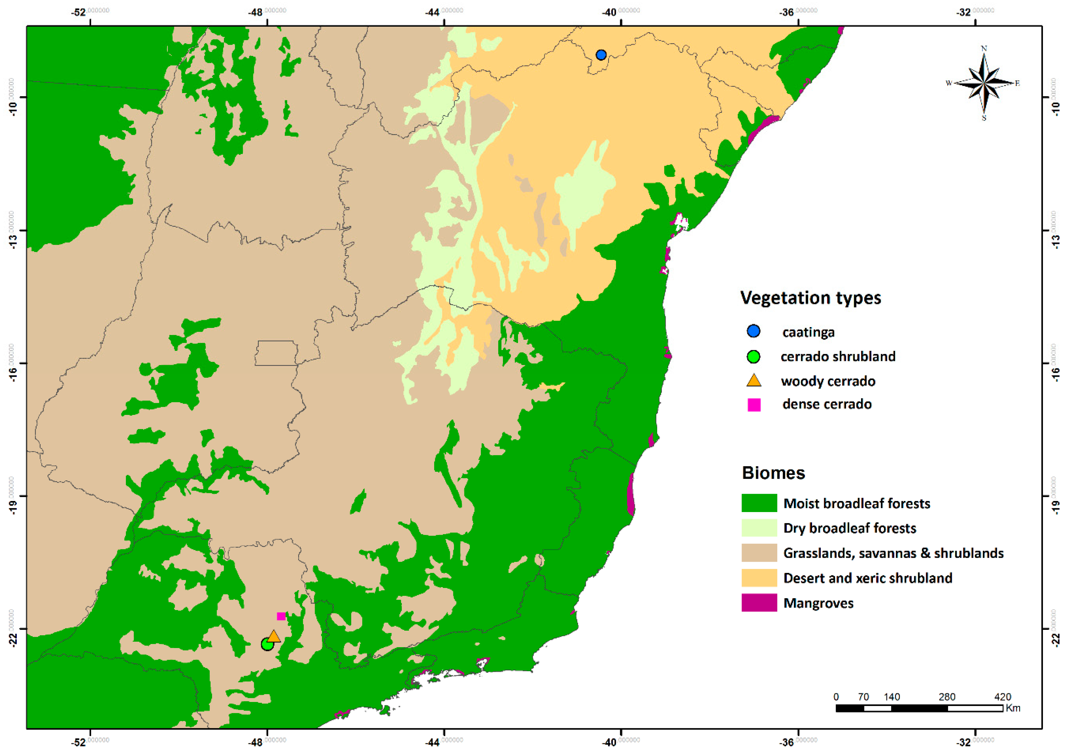
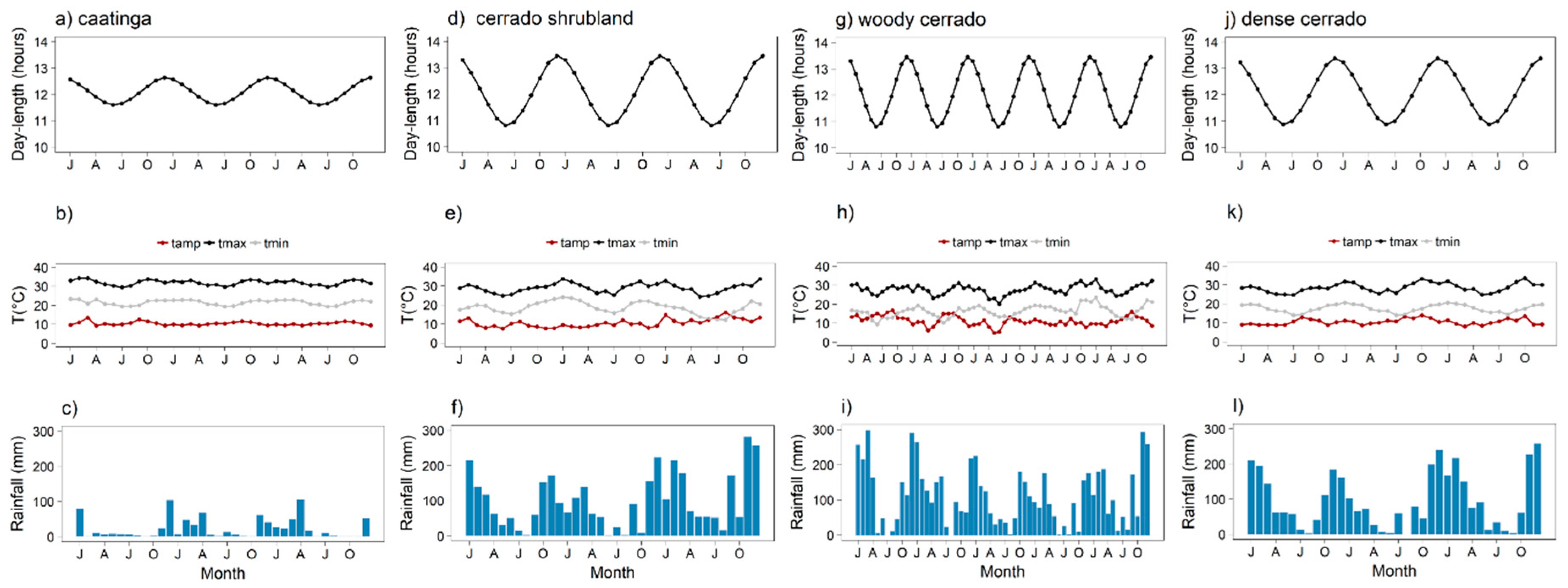
• Cerrado shrubland—the cerrado shrubland (campo sujo) is characterized by a dominant grassy herbaceous layer with scattered shrubs and small trees [24,42]. This site is part of the Itirapina Ecological Station, with an area of 2300 ha and an altitude of 700 m. Previous vegetation surveys found that 79% of the species from the herbaceous-shrubland layer belong to Asteraceae, Fabaceae, Poaceae, and Cyperaceae, and 21% of the small tree species were mainly from Fabaceae, Myrtaceae, and Melastomataceae [43]. As reported by [44], local historic climatic data show a total mean annual precipitation of 1524 mm and mean temperature of 20.7 °C. During the three years we monitored the area, the mean annual precipitation was 1272 mm and a mean annual temperature 23.5 °C (Figure 2e,f). Historic climatic information was made available by the Centro de Recursos Hídricos e Estudos Ambientais (CRHEA-EESC/USP), located about 15 km from the study sites.
• Woody cerrado—this site is located in a private area of 260 hectares and 700 m a.s.l. adjacent to the cerrado shrubland site. This woody cerrado is a remnant of the original Cerrado that once covered the entire region, and therefore, faces the same climatic regime as the cerrado shrubland site. The vegetation is a cerrado sensu stricto, which is characterized by a dominant woody layer (trees and shrubs ranging from 3 to 12 m in height) with discontinuous crown cover and a scattered herbaceous layer [44]. According to local meteorological data (2011–2015), mean annual total precipitation was 1478 mm and mean annual temperature 22.9 °C (Figure 2h,i). The most common plant families are Myrtaceae, Fabaceae, and Malpighiaceae [44], and the vegetation has been classified as semi-deciduous based on long-term leaf exchange strategies [4].
• Dense cerrado—this site is a dense woody cerrado that belongs to the Reserva Ecológica Pé-de-Gigante (PEG), located within the Parque Estadual do Vassununga, in Santa Rita do Passa Quatro, SP. The PEG reserve comprises a continuous area of 1060 ha and 649 m a.s.l. covered by a heterogeneous landscape of Cerrado vegetation types, from open grasslands to dense woody cerrado. As reported by Batalha et al. [24], local climatic data (1986–1995) presented a total mean annual rainfall of 1499 mm and mean annual temperature of 21.5 °C. Our local climatic data (2013 to 2015) showed a total mean annual precipitation of 1150 mm and a mean annual temperature of 22.5 °C (Figure 2k,l). The study site is a transition from woody cerrado to cerradão [42], which we classified as dense cerrado; it is characterized by a less discontinuous top canopy, nearly no herbaceous layer, and a high density of shrubs and trees [45]. Dominant woody layer reaches 10 to 15 m height is composed mainly of Ptedoron pubecens, Copaifera langsdofii, and Anadenanthera peregrina var. falcata (all Fabaceae) [46].

2.2. Near-Surface Phenology Monitoring

For each study site, a digital hemispherical Mobotix Q 24 lens camera (Mobotix AG—Germany) was placed in a tower attached to an extension arm facing northeast (east for the caatinga site) at a mean vertical distance of 10 m (6 m for the caatinga site) from the top of the canopy. At the caatinga and dense cerrado study sites, the local flux towers measure 16 and 26 m, respectively; the phenological tower at woody cerrado measures 18 m. At the cerrado shrubland, the camera system was placed at 4 m from the vegetation in a landscape standing point (see [33]). The cameras were supplied by a 12 V battery that was charged by solar panels. Cameras were set to automatically take a sequence of five JPEG images (at 1280 × 960 pixels of resolution) in the first 10 min of each h, from 6:00 to 18:00 h (UC−3; Universal Time Coordinated), on a daily basis, as described in Alberton et al. [32]. The camera systems were installed at different times during the monitored years (see Table 1), so we analyzed the period ranging from 2013 to 2015 for all sites except the woody cerrado, where the time series started in 2011 (Table 1). Due to several environment-related energy supply issues throughout the monitoring years for the woody cerrado site, we developed an algorithm to fill in gaps of more than seven days with no recorded images, using the R programming language [47] (see Supplementary material for more details).

Raw images were initially screened visually to remove photographs where canopy view was obstructed. The remaining images were analyzed as described by Richardson et al. [48], Ahrends et al. [49], and Alberton et al. [32]. We carried out field expeditions to identify plant species and compile a list of the main species captured by the field of view of each camera (see Supplementary material). We then matched the identified individuals with the crowns observed in the images. This information, associated with visual image inspections, was essential to properly classify the individual crowns into plant functional groups based on leaf exchange strategies and to confirm the phenological transition dates.

Regions of interest (ROIs) were defined in the images of each site to capture the community as well as separate deciduous species (for cerrado areas only; based on [4]), and grass versus woody cover (for cerrado shrubland only). The community ROIs refer to the entire community present in the image (ROI = entire image excluding the tower and bare soil patches); deciduous ROIs refer to all deciduous crowns observed in the image (cerrado shrubland = 16.16%; woody cerrado = 5.44%; dense cerrado = 21.5%); grass ROIs refer to the herbaceous cover observed in the cerrado shrubland (23.70%). The proportion of deciduous species and grass cover was determined by the percentage of pixels in relation to the total pixels from the community ROI.

We analyzed all ROIs in terms of the contribution of the relative brightness of red, green, and blue color channels (RGB chromatic coordinates; [50]). The normalized RGB chromatic coordinate (RGB_cc) index is the most suitable index to detect leaf color changes, such as leaf development and photosynthetic dynamics, and the most efficient index to suppress light variations [32,48,49,50,51,52,53,54,55]. We thus calculated the normalized index of the green color channel (Gcc) according to the formulas:

Total_avg = (Red_avg + Green_avg + Blue_avg)

(1)

Gcc = (Green_avg)/Total_avg

(2)

The Gcc index was calculated separately for each of the five hourly images taken each day. One single measurement was then extracted by taking the 90th percentile of all values observed every three days, to minimize interferences related to lighting changes caused by weather, season, and time of day [55].

2.3. Defining the Growing Season

We extracted phenological metrics to define the growing season and to detect phenological transitions [56]. Time series of tropical communities are often more difficult to characterize temporally, as they are mostly rain-green systems [56]. To overcome problems related to the detection of green-up responses coupled with precipitation events, which result in noisier observations, we propose, for the first time, the use confidence intervals of curve derivatives to identify changes in phenology. To do so, we first fitted Generalized Additive Mixed Models (GAMM) to the Gcc community time series (see [4]). Time (sequence of days) was used as an independent smoother variable. Assuming that errors are not independent, a condition inherent to the structure of time series, we assumed an auto-regressive moving average (ARMA) correlation to our model residuals. We then generated 10,000 independent simulations of fitted curve and calculated the derivative of each simulated curve at each time step, thus building confidence intervals for the rate of changes (derivatives significantly different from zero) along the curve. A significance level of 10% was chosen due to the high variability associated with daily phenocam observation. From the derivatives, we were able to extract phenological metrics, or phenological transitions, that corresponded to significant periods of increases in greenness values, followed by a short period of no change, and then a significant period of decrease in greenness. Based on previous classifications of land surface phenology time series [57,58] and according to the traditional classification of directly observed phenological variables [7], we defined the phenological metrics as:

Start of growing season (SOS)—represents the beginning of the growing season and is measured as the first day detected by a significant derivative from the total seasonal amplitude on the left side of the curve.

End of growing season (EOS)—represents the end of the growing season and is measured as the last day detected by a significant derivative from the total seasonal amplitude on the right side of the curve.

Length of growing season (LOS)—represents the duration of the growing season and is calculated as the difference between SOS and EOS.

Peak of growing season (POS)—represents the highest greenness percentage, generally associated to the highest percentage of species flushing new leaves. It is measured as the highest value of the seasonal curve.

2.4. Environmental Cues of Leafing Phenology

Photoperiod, temperature, water availability, and water-energy interactions [59] were chosen as the potential environmental factors to characterize leafing phenological patterns across sites. The set of explanatory variables was selected based on a priori assumptions and on information extracted from the literature.

At the caatinga and dense cerrado study sites, environmental data was measured with sensors installed in the local flux towers where phenocams were set up. A CR1000 datalogger (Campbell Scientific Inc.) was used to calculate averages of 30-s measurements at each 30-min interval between May 2013 and December 2015 for the caatinga site and between August 2013 and December 2015 in the dense cerrado site. For the other locations, a U30-Hobo meteorological station, installed in the phenological tower located at each site, collected all environmental variables.

Maximum and minimum daily temperatures were used to calculate the temperature amplitude along the year:

Tamp = Tmax − Tmin

(3)

Rainfall effects were tested using the following variables: cumulative precipitation, from the last 30 days (Rainfall_cum_30), and lagged rainfall events from the last seven (Rainfall_Lag7) and 30 (Rainfall_Lag30) days.

Water and energy interactions were calculated to evaluate the effects of the dry season intensity using the cumulative water deficit (cwd) according to James et al. [60]:

cwdn = (cwd_(n − 1)) + (Pn − (ETn))

(4)

where cwdn is the computed cumulative water deficit for a given time (n), Pn is the precipitation of the day (mm), and ETn is the evapotranspiration of the day (mm day⁻¹). When a positive value of (P − ET) is identified, zero is used to set a starting point. Every time cwdn ≥ 0, then cdwn is set to zero again (more details in [59,60,61]). Interactions between evapotranspiration demand, which is induced by the amount of energy in the system (able to heat and/or stress the plant), and water availability in the soil are explained by the climatic water balance (see [59]). When evaporative demand is higher than the amount of water available, a deficit occurs, which explains the cwd (a measure of absolute drought) [59,60,61]. Evapotranspiration was calculated by the eddy covariance method in the caatinga and dense cerrado sites. For cerrado shrubland and woody cerrado, we used the evapotranspiration value of the CRHEA-EESC/USP meteorological station (located 10 km away from the sites).

Day-length (the number of sunlight hours) was chosen to represent photoperiod seasonality and was calculated using the latitude of each location (geosphere package in R). The environmental variables were aggregated into three-day windows using the same percentile approach applied to the greenness series [55].

2.5. Data Analysis

Phenological metrics were extracted from the community Gcc time series and compared among vegetation types. To investigate the relationship between leafing phenology and environmental cues, we fitted separate Generalized Additive Mixed Models (GAMMs) using the community Gcc time series, leaf exchange strategy, and dominant life-forms as dependent variables (Y) and the abiotic environmental data as explanatory variables (X). We used GAMM as they are able to capture nonlinear relationships across multiple covariates, reliably handle structural time series in ecological studies and vegetation modeling [62,63,64].

The general formula of a GAM is:

g(μ) = ∑f(X)

(5)

Where g is a specified link function, (μ) the expected mean response, and ∑f(X) are smooth functions of the covariates (X) [65]. Basically, GAMs aim to maximize the quality of the prediction (μ) by estimating non-parametric functions of the predictor variables (X) through connections with the dependent variable that are established by a link function (g) [63,66]. The Generalized Additive Mixed Model (GAMM) approach adds a random factor into the general GAM formula. Since we are dealing with time series (Gcc) and assuming that errors are not independent, an auto-regressive moving average (ARMA) correlation structure was nested into the models.

Initially, scatterplots among covariates were verified to identify linear and non-linear relationships. After running multicollinearity inspection, we used a full model for each dependent variable where we entered all chosen explanatory variables. Variable selection, which means a smooth component selection when working with GAMMs, was carried using a shrinkage approach, denominated double penalty, which relies on the fact that the space of the smoother (a spline basis) can be decomposed into components: range space and null space [66]. The method penalizes both components shrinking them to zero. By introducing a penalty in the null space, the GAMM smoothing estimator can select the most significant terms from the model (for more details about the method, see [66]). By analyzing the approximate smooth estimators from the model, we can identify terms that are not statistically significant (significance with p values < 0.001) and remove them altogether. Finally, to understand how each term is interacting with the response variable, we interpreted plots of the partial fits of each smoother parameter and evaluated F-tests of model outcomes.

3. Results

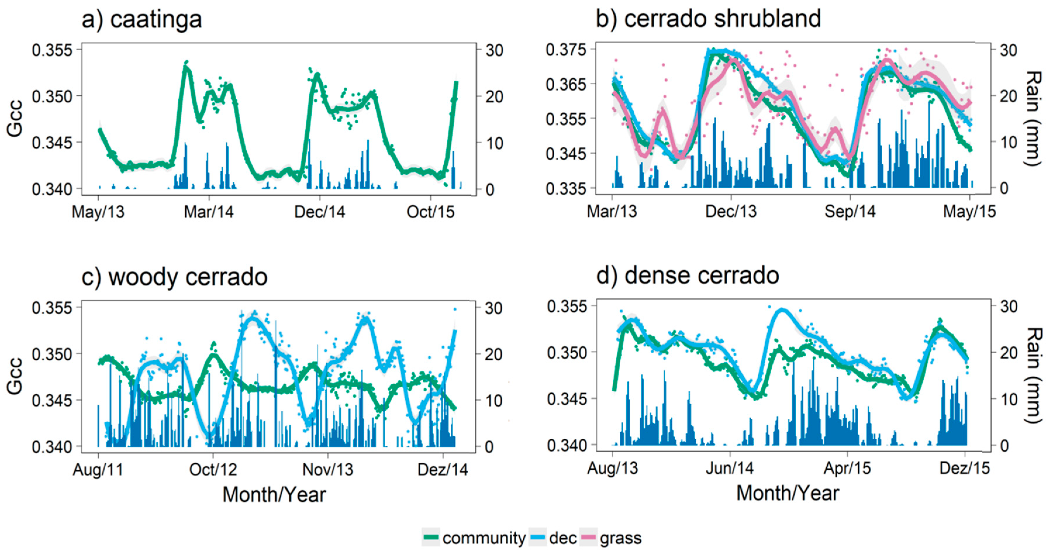
3.1. Detecting Growing Seasons Across Sites

The Gcc index calculated for the community time series tracked the seasonality of leafing patterns in all sites (Figure 3). Using the derivatives, we were able to find the timing of leafing phenological transitions for all annual cycles (Table 2). In general, growing seasons differed among vegetation types mainly in relation to the start and end dates, season length, and shape of the seasonal curves, which are related to the characteristic leafing response of each community.

The start of the growing season (SOS) occurred earlier for cerrado vegetation types in comparison to the caatinga, and ranged from day of the year (DOY) 147 to DOY 239 (Table 2). The woody cerrado had the earliest SOS (mean DOY = 163), occurring mid-June (mid-dry season). SOS in the dense cerrado and cerrado shrubland were similar and occurred in August (mean DOY 221 and 233, respectively). SOS in the caatinga occurred by the end of October (mean DOY 296), after the first rainfall events. All communities reached the peak of their growing season (POS) about 78 days after their SOS. Caatinga and dense cerrado were the first to reach their POS (69 and 67 days, respectively), while the cerrado shrubland and the woody cerrado reached their POS later (80 to 96 days, respectively). For the two wooded cerrado vegetation types, POS occurred during the dry-to-rainy season transition, contrary to the caatinga and cerrado shrubland, where POS dates occurred within the rainy season.

The end of the growing season (EOS) occurred faster and earlier in the caatinga vegetation, and the difference between the first (2013/2014 = 183) and the second (2014/2015 = 214) cycles was of about a month (31 days; Table 2, Figure 3). The length of the growing season (LOS) was also the shortest in the caatinga, with a mean LOS of 274 days. Additionally, green-down was more abrupt and EOS occurred immediately after the end of the rainy season (Figure 3a). Conversely, cerrado vegetation types showed a slower transition and extended green-down curve, reaching the lowest values from the mid to the end of the dry season (Figure 3b–d). The woody cerrado showed different EOS across years, ranging from mid-May (DOY 134 in 2012/21013) to mid-June (DOY 170 in 2011/2012), and LOS also varied from 314 to 342 days. Only one LOS was recorded for the cerrado shrubland and the dense cerrado sites (a single complete cycle), and both sites had the longest LOS, with 345 days.

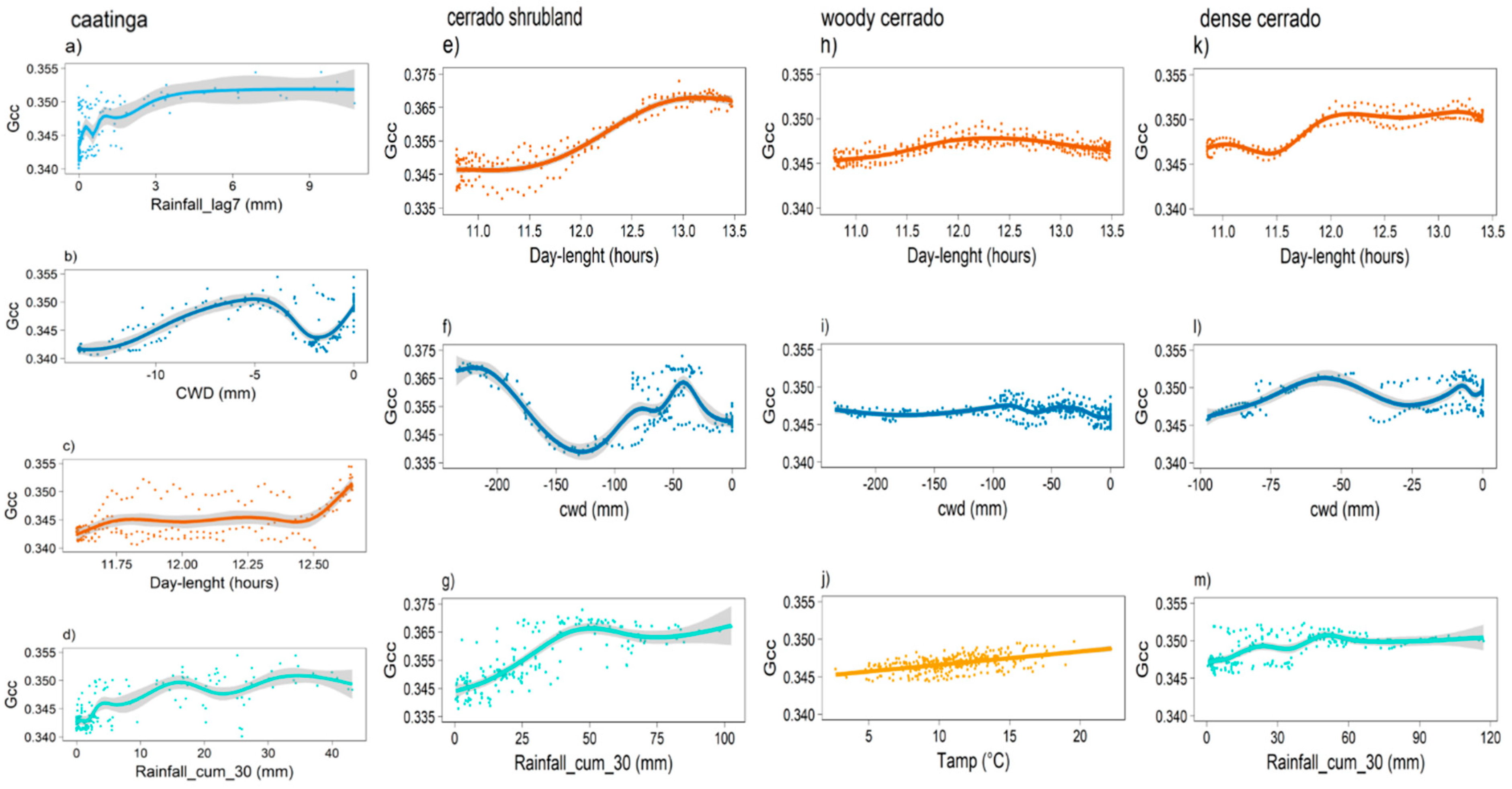
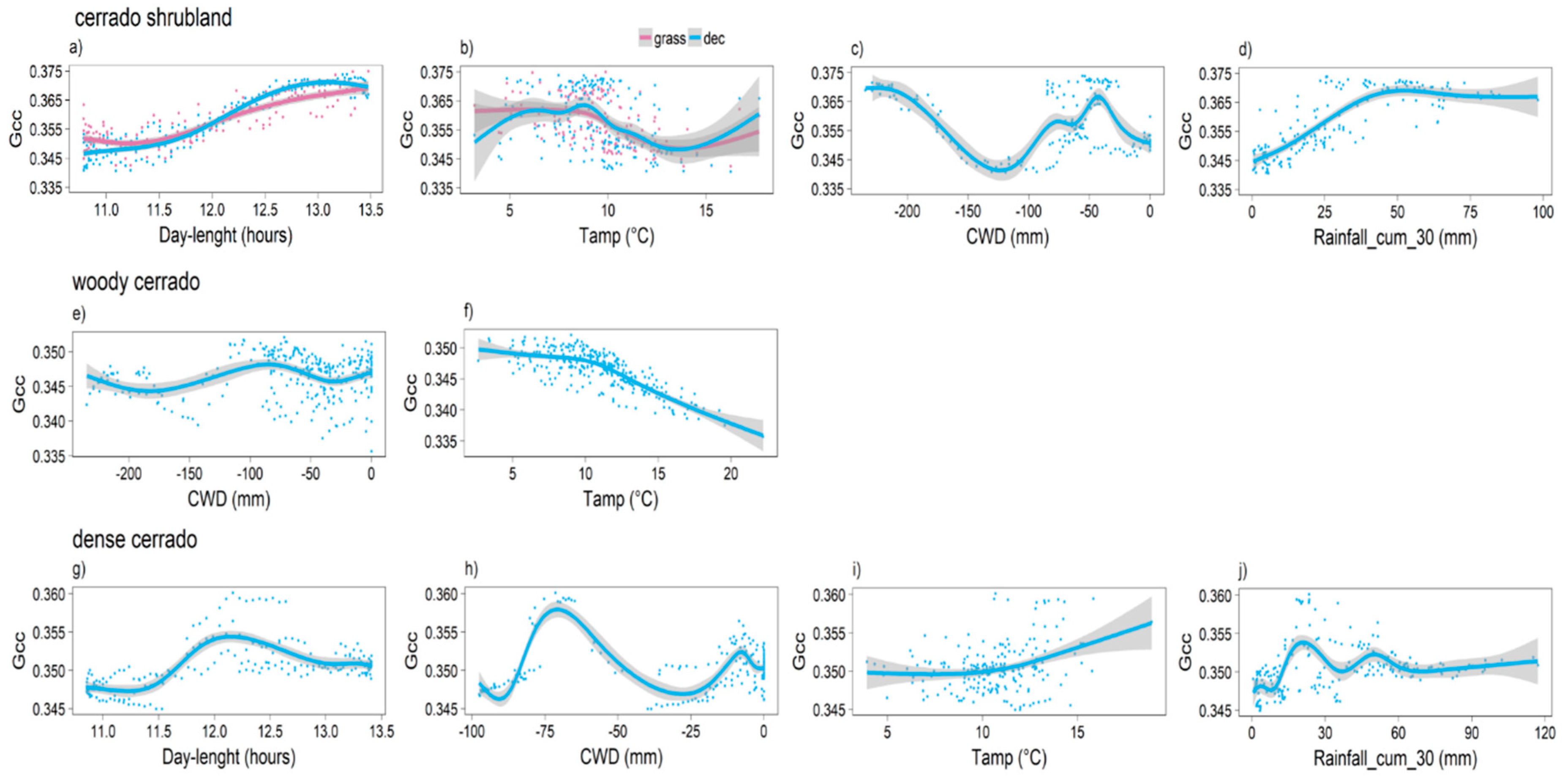
3.2. Model Predictions

Predictor variables were selected as smooth terms in most of the models. Two of the explanatory variables had linear relationships when modeled against the ROI data: Rainfall_lag7 in the caatinga and Tamp in the woody cerrado. In general, the GAMMs produced models with medium to high explanation power (R² from 0.29 to 0.88). Day-length and cwd were the most recurrent predictors, with the highest statistical significance values across all vegetation types (

Table 3. Approximate significance of the smooth terms used in the GAMMs. Effective degrees of freedom (edf) and F-test values are given for each of the following variables: day-length, cumulative water deficit (cwd), precipitation lagged seven days (Raifall_lag7), cumulative precipitation from the last 30 days (Rainfall_cum_30), and thermal amplitude (Tamp). The coefficient of determination (R²) of each model is also shown. All variables were significant, with p values < 0.001. comu = community; dec = deciduous; grass = grassy layer. ROI: region of interest.

Site Location	ROI	Day-Length (Hours)		cwd (mm)		Rainfall_ lag7days (mm)		Rainfall_Cum_30days (mm)		Tamp(oC)		R2
		edf	F-Test	edf	F-Test	edf	F-Test	edf	F-Test	edf	F-Test
Caatinga	comu	7.83	12.324	8.559	28.565	1.0	36.02	6.91	16.36	N. S	N. S	0.86
Cerrado shrubland	comu	5.726	39.535	6.678	13.189	N. S	N. S	3.907	4.617	N. S	N. S	0.88
	grass	2.114	9.535	N. S	N. S	N. S	N. S	N. S	N. S	1.00	19.531	0.56
Woody cerrado	comu	7.773	36.383	7.94	8.317	N. S	N. S	6.745	3.156	N. S	N. S	0.79
	dec	7.144	30.9	8.264	28.548	2.719	6.734	5.884	3.857	1.00	6.772	0.82
Dense cerrado	comu	5.218	22.436	7.097	8.484	N. S	N. S	N. S	N. S	3.558	17.051	0.51
	dec	N. S	N. S	7.665	5.904	N. S	N. S	N. S	N. S	3.663	25.488	0.42

). However, other variables were also significant in explaining leaf phenology according to the GAMMs (Figure 3 and Figure 4). The most important relationships are described in more detail below.

For caatinga, the variables that best explained community greening (Gcc) were cwd and rainfall (lag7 and cum30) (Figure 4a,b). The partial fit between predictors and Gcc demonstrated that vegetation was sensitive to low values of precipitation and to cwd values between −10 and −5, which caused an increase in Gcc values (Figure 4b). Day-length, also included in the model as a significant variable (Table 3), started to affect the community Gcc after 12.5 h of sunlight.

For the three cerrado vegetation sites, day-length was the variable that best explained community Gcc patterns (Table 3). The same values, ranging from 11.5 to 12.0 h, were observed as a sensitive threshold for phenological transitions across all vegetation types (Figure 4e,h,k). Cwd resulted in different smooth functions among cerrado sites, where cerrado shrubland and dense cerrado were strongly sensitive to cwd with green-down values between −150 and −100 (Figure 4f,l), while woody cerrado was less sensitive (Figure 4i).

Cumulative rainfall (Rainfall_cum_30) was significant for both cerrado shrubland and dense cerrado (Table 3), indicating that changes in Gcc can occur in both vegetation types when values of accumulated precipitaton rates are between 25 to 30 mm (Figure 4g,m). The Gcc time series from the woody cerrado community was the only one that interacted with thermal amplitude (Tamp—3.558, 17.05, P < 0.001, Table 3). There was a positive linear relationship between the covariates, where Gcc values increased as Tamp increased (Figure 4j).

The ROIs separating deciduous leaf exchange strategies and life forms (grassy layer) interacted with different variables across vegetation types. We compared the deciduous ROIs among sites, but since the overall caatinga community displays a deciduous behavior, we used the community ROI for the caatinga (and not the deciduous ROI) to carry out such comparisons. The relationship between the community Gcc patterns and precipitation events were higher in the caatinga, followed by the cerrado shrubland, woody cerrado, and, finally, dense cerrado (Figure 5). Particularly, the caatinga vegetation showed a pattern of fast response to water availability, with pulses of green-up following rainfall events (Figure 5a). Among the cerrado vegetation types, the Gcc curve of the cerrado shrubland was better linked to precipitation in comparison to curves from the woody and dense cerrados, mainly when considering the Gcc curve oscillations (Figure 5b–d).

The deciduous ROI curves from the cerrado sites showed variable patterns. The deciduous shrub layer from the cerrado shrubland followed a pattern similar to the community pattern, with an overlap of green-up and green-down periods (Figure 5b). Conversely, the deciduous ROI curve from the woody cerrado showed green-up within the rainy season, with high values of Gcc still during the dry season (Figure 5c). In the dense cerrado, green-up occurred during the dry season before the first rainfall events, reaching its peak in the transition between the dry and rainy seasons (Figure 5d). The grass ROIs had green-up curves similar to the community and to the deciduous species but peaked during the rainy season. The grassy component also showed marked fluctuations within the rainy season, apparently following individual rainfall events, even though we observed the highest peak during the dry season (Figure 5b).

Among the cerrado vegetation types, we observed that leafing strategy interacted with different environmental variables. In the cerrado shrubland, cwd and cumulative rainfall (Rainfall_Cum_30) interacted exclusively with the green-up pattern of the deciduous ROI (Figure 6c,d). Cwd values between −100 and −150 mm led to green-down events, and green-up events only began after cwd values over −100 mm. The variables day-length and Tamp also significantly affected the green-up and green-down patterns. Tamp between 5 and 10 °C increased Gcc, which decreased after a Tamp over 10 °C. (Figure 6a,b). In the woody cerrado, the variables cwd and Tamp significantly affected the deciduous ROI model, with green-up being positively affected by the decrease in water defict (below −100 mm) and negatively affected by Tamp over 10 °C (Figure 6e,f). In the dense cerrado, the curve inflection of deciduous ROI was sensitive to day-lengths between 12.0 to 12.5 h (Figure 6g). Cumulative rainfall (Rainfall_Cum_30) and cwd showed peaks of increasing green-up when values ranged from 15 to 30 mm and −75 to −50 mm, respectively (Figure 6h,j).

The grass layer from the cerrado shrubland was significantly related to day-length, where a positive linear relationship was established with day-lenth over 11.5 h, while with Tamp the curve showed an inverse sigmoid relationship (Figure 6a,b).

4. Discussion

4.1. Communities Leafing Patterns

The Gcc index extracted from the digital images allowed us to track leafing seasonality in the studied tropical seasonal communities and determine the growing season using phenological metrics detected from the derivatives of fitted generalized additive mixed models. As expected, Gcc curves coincided with the rainy season, leading to differences in growing season and phenological transitions among vegetations, especially between the caatinga and the cerrado vegetation types. For the woody and dense cerrado, the beginning of the growing season (SOS) and their peak (POS) occurred during the dry season, while for the caatinga and the cerrado shrubland, leaf flushing began with the first rainfall events and reached its peak within the rainy season. According to our results, environmental responses of community leafing patterns change gradually across these vegetation types, with the caatinga as the most water-responsive vegetation, followed by the cerrado shrubland, which shows important day-length and water-related responses, and finally both wooded cerrado communities, where day-length was the main variable affecting the onset of the growing season.

The shape of growing season curves differed among vegetation types and were clearly influenced by water availability throughout the year, leading to a variation in the length of the growing season (LOS): much shorter in the caatinga in comparison to the cerrado sites. Green-up and green-down curves were more abrupt for the caatinga, which may be explained by the predominance and synchronicity of seasonally deciduous species that occur in these environments [10,65]. Conversely, the mild dry season observed for the Cerrado favors a different proportion of deciduous, semi-deciduous, and evergreen species. Green cover in Cerrado is maintained even during the dry season and Gcc curves change throughout the rainy season. Our findings support the direct observations of leaf exchange patterns that have been previously determined at the woody cerrado site and the classification of the Cerrado vegetation as a semi-deciduous vegetation [4,67]. Community green-down patterns for the shrubland and woody cerrado sites started at the end of the rainy season (represented by the last Gcc oscillation before the descending pattern of the terminal derivative), while in the dense cerrado green-down occurred from the second Gcc oscillation after the peak. Such decreasing values of Gcc (from the peak date until the beginning of senescence) correspond to the period of leaf maturation. Thus, Gcc index is sensitive to leaf color changes [68] and there is a gradual color change with the ageing of community leaves (see Methods).

The interannual variation in SOS and EOS dates was higher in the caatinga (SOS differed 28 days between years and EOS differed 31 days) and in the woody cerrado (SOS differed 38 days between years and EOS differed 36 days). For the caatinga, the Atlantic Dipole phenomenon (a temperature variation of the Atlantic Ocean) causes high interannual variability in precipitation rates [69], which would lead to shifts in seasonality dynamics of the growing season among years. According to our models and given that plant species from the caatinga are influenced mainly by water availability, there is an immediate response in both reproductive and vegetative phenology after rainfall events, given these events determine the onset of the rainy season [70,71]. Regarding the woody cerrado, studies usually report that leaf flushing (SOS) begins at the end of the dry season or during the dry-to-rainy season transition [4,11,72,73,74]. Among woody cerrado species, our results indicate two main leaf flushing strategies: species either respond to the first rains that occur during the dry-to-rainy season transition or leaf flushing begins still during the dry season (see [4] for further discussions). Similarly, leaf flushing of shrubland cerrado species began during the dry season; however, their POS dates differed from the woody cerrado community as it occurred during the rainy season, probably due to the dominant grass layer.

Our model predicted non-linear relationships between phenology and the recurrent significant variables: day-length and cwd. The skewness pattern of greening in the caatinga indicates there is a link between time and duration of the irregular leafing cycles, which are restricted to the rainy season and follow the precipitation pulses that occur in the system. Thresholds in plant-water relationships indicate that Gcc changes are stimulated by low rates of accumulated precipitation, which explains the fast response of leaf flushing observed for caatinga species.

Day-length was the most common variable explaining Gcc patterns for cerrado communities. Increasing day-length (longer days) triggers leaf flushing of most cerrado species in the communities studied, starting early in the dry season. Photoperiod has been reported to trigger leaf flushing in seasonal dry tropical vegetation [8,19,75,76,77], but studies in the Brazilian caatinga are still lacking [78].

The community leaf flushing peak occurring before the onset of the rainy season supports the hypothesis that cerrado woody species have access to underground water, due to deep root systems, or are able to rehydrate themselves by using water from leaves of the previous cycle [79,80]. Consistent photoperiod signals have been suggested to trigger and synchronize leaf flushing in the tropics, even though species show different leaf exchange strategies [4,8,76,81] even in non-seasonal systems [7]. Community leaf flushing before the rainy season would also avoid the higher herbivory rates that occur during the rainy season and the leaching-induced nutrient loss during leaf development, given nutrient uptake would take place before the rains [4,82,83].

The cwd relationships also explained the seasonality of leaf production in all four seasonally dry tropical communities investigated in this study. Its relationship with the Gcc time series in the caatinga was subtle when compared to the relationships observed in the cerrado sites, which corroborates that caatinga species are sensitive to the slightest increase in water availability. Cwd showed similar patterns across the three cerrado sites, with green-down occurring when water deficits were high (−150 mm to −100 mm) and green-up with cwd around −50 mm. Cumulative water deficits are essential in understanding plant physiological responses given that it integrates water and energy interactions [59]. Additionally, cwd is related to drought stress experienced during the dry period [60,61]. Global scale studies have proposed a threshold of 2000 mm of annual rainfall in tropical forests in order to sustain water demands and keep the evergreen state of species throughout the year [12,84]. In Cerrado species, the dry season has been stated as a key factor triggering vegetative phenological transitions, affecting leaf abscission and leaf emergence [85].

The 30-day cumulative rainfall (Rainfall_cum_30), which was present in all models, explained the community leafing patterns in all sites except for the woody cerrado. In comparison with the caatinga, the cerrado sites needed twice as much cumulative rainfall to stimulate increases in Gcc. These results indicate the role water availability plays in leafing patterns of cerrado species, where day-length acts as a first trigger, stimulating leaf unfolding, and rainfall intensity acts as a driver of leaf expansion, thus avoiding drought limitations during drier periods [86,87]. Contrarily, in the woody cerrado, thermal amplitude (Tamp) was the variable that best explained the community Gcc. Tamp was also positively correlated with rates of green-up and senescence in plant communities across a snow-free mountain, which included grasslands and cerrado areas [88]. At the woody cerrado site, Tamp reached 20 °C during the dry-to-wet season transition and was also related to earlier patterns of leaf flushing.

Anticipating leaf flushing may provide major carbon gains, since species with early leaf emergence increase carbon assimilation rates once the rainy season begins [85,89,90], resulting in a longer and more productive growing season.

4.2. Deciduous Leaf Exchange Strategies and Life Forms

The deciduous component showed different patterns across the four communities: in the caatinga, all species were deciduous, while the cerrado shrubland was composed of a deciduous woody component and a grassy layer and, in the two wooded cerrado sites, the deciduous component decreased—deciduous ROI cover was around 6% at the woody cerrado and 20% at the dense cerrado. The proportion of deciduousness is reflected in the degree of seasonality of the community Gcc time series across sites, from the marked seasonal caatinga, followed by the cerrado shrubland with a deciduous woody component to the woody cerrado. The factors affecting the proportion of the deciduous component coincide with the results found for the entire community, where woody cerrado species are less water-dependent in comparison with caatinga and cerrado shrubland species.

The caatinga was the most synchronous plant community, with all deciduous species responding simultaneously to cumulative rainfall. Such high synchronicity suggests that a common climatic factor triggers leaf phenological transitions, which could be explained by the strong water-response relationship. Opportunistic drought deciduous species (ODDS) are mainly driven by water availability with leaf flushing following the first rainfall events [91]. Seasonally harsh climatic conditions, characteristic of the caatinga, suggests a dominance of ODDS, with synchronic leaf flushing occurring after the first rainfall events at the end of the dry season [10,11,16,91]. The interannual variation of rainfall amount and distribution likely determines community leaf flushing and its intensity [92].

However, plant species from relatively more moderate environments, such as the cerrado, may be able to cope with water limitations and produce new leaves still during the dry season [93]. For instance, the deciduous leafing behavior from the woody cerrado was more affected by day-length than water availability. Cerrado trees use deep roots to exploit deeper soil water sources, which enables them to flush new leaves before the rainy season [23,76,94]. Schedule drought deciduous species (SDDS) are those able to endure drought conditions by maximizing their carbon gain without experiencing stress and are mainly driven by photoperiod, with high synchronicity and low interannual variability [4,22,91,95]. The persistent greening during the dry season indicates a longer resistance to drought limitations and a dominance of SDDS, even though the main drivers for deciduousness in the woody cerrado were cwd and Tamp.

In the cerrado shrubland, leaf phenology of the grassy layer was not predicted by water relationships, contradicting our expectations regarding the temporal niche separation hypothesis [36] and the water constraints imposed on phenological responses among grass species [43,96]. The grass ROI model was partially (50%) explained by day-length and Tamp. The reponse suggests the influence of invasive African grasses, particularly Melinis minutiflora and Urochloa brizantha, which are extremely abundant in the area [43,97]. The isolated greening event that occurred during the dry season, observed in both yearly cycles, could be an indication of the effect invasive species had on our results. The anticipated green-up event may have caused the low correlation with rainfall covariates from the model, as leafing of invasive species began before the rainy season and, thus, before native graminoids. The anticipation suggests the priority effects hypothesis, which states that an earlier establishment in the growing season benefits invasive species as they will use resources first [98], and explains the phenological behavior of such species [98]. Additionally, the rapid evolution of phenology may be a widespread and essential process during the expansion of many invasive species [99]. However, studies comparing the phenological behavior of invasive and native grasses are still lacking, hindering adequate management actions.

Our results demonstrated that phenological leaf exchange dynamics in seasonally constrained environments tend to be more synchronic, since caatinga and grass species are adapted to flush during a limited but favorable period for plant development (rainy season). As the environment becomes less constrained by climate (mild dry season), leaf exchange patterns become less restricted to the rainy season [100], allowing leaf flushing to begin in the dry season.

5. Conclusions

We found that water and light are the most important predictors for leaf phenological patterns across seasonally dry environments (caatinga and cerrado). For caatinga, short cumulative seven-day rainfall events were able to initiate the growing season and leaf flushing. Day-length and cwd were the most influential factors across cerrado sites, regardless of leaf exchange strategies. Degree of seasonality, which is related to the length and intensity of the dry season, reflected on community leafing patterns and on what drives the deciduous component of these communities. While deciduous species from the xeric caatinga were responsive to cumulative water availability, the woody deciduous species of cerrado were responsive to day-length. The absence of rainfall covariates in the grass model suggests the interference of invasive grasses. Understanding leaf phenology mechanisms are essential to effectively forecast future Earth systems. The results reported here contribute to detect leaf flushing and senescence transitions, their main drivers, and the thresholds affecting them. Thus, our findings contribute to understand the dynamics of tropical seasonal communities across areas with varying water dependence. The effects of anthropogenic climate changes in the tropics are predicted to result in longer and more intense dry seasons [89,90]. The increase of aridity during the dry season has been reported to cause greater impacts over productivity than the excess of water, seasonally or annually, could cause [61,101]. The impact of more intense dry seasons would be bigger in deciduous species as they are more sensitive to seasonal climatic variations. A major impact is expected for the deciduous caatinga species given the strong water-dependence. Cerrado species, triggered by day-length, would continue to flush new leaves in the dry season; however, dryness could affect the full development of leaves and shorten the growing season, which would anticipate senescence. Non-deciduous species, a significant part of cerrado communities [4], would also be affected since the increase of aridity reduces C gain, affecting productivity [61,83,101].

References

1. Reich, P.B. Phenology of tropical forests: Patterns, causes, and consequences. Can. J. Bot. 1995, 73, 164–174. [Google Scholar] [CrossRef]
2. Rötzer, T.; Grote, R.; Pretzsch, H. The timing of bud burst and its effect on tree growth. Int. J. Biometeorol. 2004, 48, 109–118. [Google Scholar] [CrossRef]
3. Richardson, A.D.; Keenan, T.F.; Migliavacca, M.; Ryu, Y.; Sonnentag, O.; Toomey, M. Climate change, phenology, and phenological control of vegetation feedbacks to the climate system. Agric. For. Meteorol. 2013, 169, 156–173. [Google Scholar] [CrossRef]
4. Camargo, M.G.G.; Carvalho, G.H.; Alberton, B.C.; Reys, P.; Morellato, L.P.C. Leafing patterns and leaf exchange strategies of a cerrado woody community. Biotropica 2018, 50, 442–454. [Google Scholar] [CrossRef]
5. Van Schaik, C.P.; Terborgh, J.W.; Wright, S.J. The Phenology of Tropical Forests—Adaptive Significance and Consequences for Primary Consumers. Annu. Rev. Ecol. Syst. 1993, 24, 353–377. [Google Scholar] [CrossRef]
6. Wright, S.J.; van Schaik, C.P. Light and the Phenology of Tropical Trees. Am. Nat. 1994, 143, 192–199. [Google Scholar] [CrossRef]
7. Morellato, L.P.C.; Talora, D.C.; Takahasi, A.; Bencke, C.C.; Romera, E.C.; Ziparro, V.B. Phenology of Atlantic Rain Forest Trees: A Comparative Study. Biotropica 2000, 32, 811–823. [Google Scholar] [CrossRef]
8. Rivera, G.; Elliott, S.; Caldas, L.S.; Nicolossi, G.; Coradin, V.T.; Borchert, R. Increasing day-length induces spring flushing of tropical dry forest trees in the absence of rain. Trees 2002, 16, 445–456. [Google Scholar] [CrossRef]
9. Borchert, R.; Calle, Z.; Strahler, A.H.; Baertschi, A.; Magill, R.E.; Broadhead, J.S.; Kamau, J.; Njoroge, J.; Muthuri, C. Insolation and photoperiodic control of tree development near the equator. New Phytol. 2015, 205, 7–13. [Google Scholar] [CrossRef]
10. Murphy, P.G.; Lugo, A.E. Ecology of Tropical Dry Forest. Rev. Ecol. Syst. 1986, 17, 67–88. [Google Scholar] [CrossRef]
11. Williams, R.J.; Myers, B.A.; Muller, W.J.; Duff, G.A.; Eamus, D. Leaf phenology of woody species in a north Australian tropical savanna. Ecology 1997, 78, 2542–2558. [Google Scholar] [CrossRef]
12. Guan, K.; Pan, M.; Li, H.; Wolf, A.; Wu, J.; Medvigy, D.; Caylor, K.K.; Sheffield, J.; Wood, E.F.; Malhi, Y.; et al. Photosynthetic seasonality of global tropical forests constrained by hydroclimate. Nat. Geosci. 2015, 8, 284–289. [Google Scholar] [CrossRef]
13. Reich, P.B.; Borchert, R. Water Stress and Tree Phenology in a Tropical Dry Forest in the Lowlands of Costa Rica. J. Ecol. 1984, 72, 61–74. [Google Scholar] [CrossRef]
14. Quesada, M.; Sanchez-Azofeifa, G.A.; Alvarez-Añorve, M.; Stoner, K.E.; Avila-Cabadilla, L.; Calvo-Alvarado, J.; Castillo, A.; Espírito-Santo, M.M.; Fagundes, M.; Fernandes, G.W.; et al. Succession and management of tropical dry forests in the Americas: Review and new perspectives. For. Ecol. Manag. 2009, 258, 1014–1024. [Google Scholar] [CrossRef]
15. Singh, K.; Singh, D.V. Effect of rates and sources of nitrogen application on yield and nutrient uptake of Citronella Java (Cymbopogon winterianus Jowitt). Fertil. Res. 1992, 33, 187–191. [Google Scholar] [CrossRef]
16. Borchert, R. Soil and stem water storage determine phenology and distribution of tropical dry forest trees. Ecology 1994, 75, 1437–1449. [Google Scholar] [CrossRef]
17. Morellato, L.P.C.; Rodriguez, R.R.; Leitão-Filho, H.F.; Joly, C.A. Estudo comparativo da fenologia de espécies arbóreas de floresta de altitude e floresta mesófila semidecídua na Serra do Japi, Jundiaí, São Paulo. Rev. Bras. De Botânica 1989, 12, 85–98. [Google Scholar]
18. Singh, K.P.; Kushwaha, C.P. Emerging paradigms of tree phenology in dry tropics. Curr. Sci. 2005, 89, 964–975. [Google Scholar]
19. Higgins, S.I.; Delgado-Cartay, M.D.; February, E.C.; Combrink, H.J. Is there a temporal niche separation in the leaf phenology of savanna trees and grasses? J. Biogeogr. 2011, 38, 2165–2175. [Google Scholar] [CrossRef]
20. Archibald, S.; Scholes, R.J. Leaf green-up in a semi-arid African savanna –separating tree and grass responses to environmental cues. J. Veg. Sci. 2007, 18, 583–594. [Google Scholar] [CrossRef]
21. Whitecross, M.A.; Witkowski, E.T.F.; Archibald, S. Savanna tree-grass interactions: A phenological investigation of green-up in relation to water availability over three seasons. S. Afr. J. Bot. 2017, 108, 29–40. [Google Scholar] [CrossRef]
22. Elliott, S.; Baker, P.J.; Borchert, R. Leaf flushing during the dry season: The paradox of Asian monsoon forests. Glob. Ecol. Biogeogr. 2006, 15, 248–257. [Google Scholar] [CrossRef]
23. Eamus, D. Ecophysiological traits of deciduous and evergreen woody species in the seasonally dry tropics. Trends Ecol. Evol. 1999, 14, 11–16. [Google Scholar] [CrossRef] [Green Version]
24. Batalha, M.A.; Mantovani, W. Reproducive Phenological Patterns of Cerrado Plant Species at the Pé-De-Gigante Reserve (Santa Rita Do Passa Quatro, Sp, Brazil): A Comparision Between the Herbaceous and Woody Floras. Rev. Bras. Biol. 2000, 60, 129–145. [Google Scholar] [CrossRef] [PubMed]
25. Caldararu, S.; Purves, D.W.; Palmer, P.I. Phenology as a strategy for carbon optimality: A global model. Biogeosciences 2014, 11, 763–778. [Google Scholar] [CrossRef]
26. Smith, P.; House, J.I.; Bustamante, M.; Sobocká, J.; Harper, R.; Pan, G.; West, P.; Clark, J.; Adhya, T.; Rumpel, C.; et al. Global change pressures on soils from land use and management. Glob. Chang. Biol. 2016, 22, 1008–1028. [Google Scholar] [CrossRef] [PubMed]
27. Chavana-Bryant, C.; Malhi, Y.; Wu, J.; Asner, G.P.; Anastasiou, A.; Enquist, B.J.; Caravasi, E.G.C.; Doughty, C.E.; Saleska, S.R.; Martin, R.E.; et al. Leaf aging of Amazonian canopy trees as revealed by spectral and physiochemical measurements. New Phytol. 2017, 214, 1049–1063. [Google Scholar] [CrossRef] [PubMed]
28. Morellato, L.P.C.; Alberton, B.; Alvarado, S.T.; Borges, B.; Buisson, E.; Camargo, M.G.G.; Cancian, L.F.; Carstensen, D.W.; Escobar, D.F.F.; Leite, P.T.P.; et al. Linking plant phenology to conservation biology. Biol. Conserv. 2016, 195, 60–72. [Google Scholar] [CrossRef] [Green Version]
29. Abernethy, K.; Busch, E.R.; Forget, P.M.; Mendoza, I.; Morellato, L.P.C. Current issues in tropical phenology: A synthesis. Biotropica 2018, 50, 477–482. [Google Scholar] [CrossRef]
30. Richardson, A.D.; Jenkins, J.P.; Braswell, B.H.; Hollinger, D.Y.; Ollinger, S.V.; Smith, M.L. Use of digital webcam images to track spring green-up in a deciduous broadleaf forest. Oecologia 2007, 152, 323–334. [Google Scholar] [CrossRef]
31. Morisette, J.T.; Richardson, A.D.; Knapp, A.K.; Fisher, J.I.; Graham, E.A.; Abatzoglou, J.; Wilson, B.E.; Breshears, D.D.; Henebry, G.M.; Hanes, J.M.; et al. Tracking the rhythm of the seasons in the face of global change: Phenological research in the 21st century. Front. Ecol. Environ. 2009, 7, 253–260. [Google Scholar] [CrossRef]
32. Alberton, B.; Almeida, J.; Helm, R.; Torres, R.S.; Menzel, A.; Morellato, L.P.C. Using phenological cameras to track the green up in a cerrado savanna and its on-the-ground validation. Ecol. Inform. 2014, 19, 62–70. [Google Scholar] [CrossRef]
33. Alberton, B.; Torres, R.S.; Cancian, L.F.; Borges, B.D.; Almeida, J.; Mariano, G.C.; Santos, J.; Morellato, L.P.C. Introducing digital cameras to monitor plant phenology in the tropics: Applications for conservation. Perspect. Ecol. Conserv. 2017, 15, 82–90. [Google Scholar] [CrossRef]
34. Crimmins, M.; Crimmins, T.M. Monitoring plant phenology using digital repeat photography. Environ. Manag. 2008, 41, 949–958. [Google Scholar] [CrossRef]
35. Brown, T.B.; Hultine, K.R.; Stelzer, H.; Denny, E.G.; Denslow, M.W.; Granados, J.; Henderson, S.; Moore, D.; Nagai, S.; SanClements, M.; et al. Using phenocams to monitor our changing earth: Toward a global phenocam network. Front. Ecol. Environ. 2016, 14, 84–93. [Google Scholar] [CrossRef]
36. Scholes, R.J.; Walker, B.H. An African Savanna: Synthesis of the Nylsvley Study; Cambridge University Press: Cambridge, UK, 1993; p. 320. ISBN 0521612101. [Google Scholar]
37. Veloso, H.P.; Filho, A.L.R.R.; Lima, J.C.A. Classificação da Vegetação Brasileira, Adaptada a um Sistema Universal; Instituto Brasileiro de Geografia e Estatística, Departamento de Recursos Naturais e Estudos Ambientais: Rio de Janeiro, Brazil, 1991; p. 124. ISBN 85-240-0384-7.
38. Olson, D.M.; Dinerstein, E.; Wikramanayake, E.D.; Burgess, N.D.; Powell, G.V.N.; Underwood, E.C.; D’amico, J.A.; Itoua, I.; Strand, H.E.; Morrison, J.C.; et al. Terrestrial Ecoregions of the World: A New Map of Life on Earth: A new global map of terrestrial ecoregions provides an innovative tool for conserving biodiversity. BioScience 2001, 51, 933–938. [Google Scholar] [CrossRef]
39. Silva, J.M.C.; Leal, I.R.; Tabarelli, M. Caatinga: The Largest Tropical Dry Forest Region in South America; Springer International Publishing AG: Cham, Switzerland, 2017; pp. 1–487. ISBN 978-3-319-68338-6. [Google Scholar]
40. Kill, L.H.P. Caracterização da vegetação da Reserva Legal da Embrapa Semiárido. Embrapa Semiárido Pet. 2017, 1, 1–27. [Google Scholar]
41. Köppen, W.P. Grundriss der Klimakunde, 2nd ed.; Walter de Gruyter: Berlin, Germany, 1931; pp. 1–369. ISBN 311112514. [Google Scholar]
42. Oliveira-Filho, A.T.; Ratter, J.A. Vegetation physiognomies and wood flora of the bioma Cerrado. In The Cerrados of Brazil: Ecology and Natural History of a Neotropical Savanna; Oliveira, P.S., Marquis, R.J., Eds.; Columbia University Press: New York, NY, USA, 2002; pp. 91–120, ASIN B0092WWFNC. [Google Scholar]
43. Tannus, J.L.S.; Assis, M.A.; Morellato, L.P.C. Fenologia reprodutiva em campo sujo e campo úmido numa área de Cerrado no sudeste do Brasil, ItirapinaSP. Biota Neotrop. 2006, 6, 1–27. [Google Scholar] [CrossRef]
44. Reys, P.; Camargo, M.G.G.; Grombone-Guaratini, M.T.; Teixeira, A.P.; Assis, M.A.; Morellato, L.P.C. Estrutura e composição florística de um Cerrado sensu stricto e sua importância para propostas de restauração ecológica. Hoehnea 2013, 40, 449–464. [Google Scholar] [CrossRef]
45. Ribeiro, J.F.; Walter, B.M.T. Fitofisionomia do Bioma Cerrado. In Cerrado: Ambiente e Flora; Sano, S.M., Almeida, S.P., Eds.; Embrapa: Brasília, Brazil, 1998; pp. 89–166. ISBN 8570750080. [Google Scholar]
46. Pivello, V.R.; Bitencourt, M.D.; Mantovani, W.; Mesquita, H.N., Jr.; Batalha, M.A.; Shida, C.N. Proposta de Zoneamento Ecológico para a Reserva de Cerrado Pé-de-Gigante (Santa Rita do Passa Quatro, SP). Braz. J. Ecol. 1998, 2, 108–118. [Google Scholar]
47. R Core Team. R: A Language and Environment for Statistical Computing; R Foundation for Statistical Computing: Vienna, Austria, 2018. [Google Scholar]
48. Richardson, A.D.; Braswell, B.H.; Hollinger, D.Y.; Jenkins, J.P.; Ollinger, S.V. Near-surface remote sensing of spatial and temporal variation. Ecol. Appl. 2009, 19, 1417–1428. [Google Scholar] [CrossRef] [PubMed]
49. Ahrends, H.E.; Etzold, S.; Kutsch, W.L.; Stoeckli, R.; Bruegger, R.; Jeanneret, F.; Wanner, H.; Buchmann, N.; Eugster, W. Tree phenology and carbon dioxide fluxes: Use of digital photography for process-based interpretation at the ecosystem scale. Clim. Res. 2009, 39, 261–274. [Google Scholar] [CrossRef]
50. Woebbecke, D.M.; Meyer, G.E.; von Bargen, K.; Mortensen, D.A. Color indices for weed identification under various soil, residue, and lighting conditions. Trans. ASAE 1995, 38, 259–269. [Google Scholar] [CrossRef]
51. Gillespie, A.R.; Kahle, A.B.; Walker, R.E. Color enhancement of highly correlated images. II. Channel ratio and “chromaticity” transformation techniques. Remote Sens. Environ. 1987, 22, 343–365. [Google Scholar] [CrossRef]
52. Migliavacca, M.; Galvagno, M.; Cremonese, E.; Rossini, M.; Meroni, M.; Sonnentag, O.; Cogliati, S.; Manca, G.; Diotri, F.; Busetto, L.; et al. Using digital repeat photography and eddy covariance data to model grassland phenology and photosynthetic CO2 uptake. Agric. For. Meteorol. 2011, 151, 1325–1337. [Google Scholar] [CrossRef]
53. Moore, C.E.; Beringer, J.; Evans, B.; Hutley, L.B.; Tapper, N.J. Tree–grass phenology information improves light use efficiency modelling of gross primary productivity for an Australian tropical savanna. Biogeosciences 2017, 14, 111–129. [Google Scholar] [CrossRef]
54. Richardson, A.D.; Hufkens, K.; Milliman, T.; Aubrecht, D.M.; Chen, M.; Gray, J.M.; Johnston, M.R.; Keenan, T.F.; Klosterman, S.T.; Kosmala, M.; et al. Tracking vegetation phenology across diverse North American biomes using PhenoCam imagery. Sci. Data 2018, 5, 180028. [Google Scholar] [CrossRef] [PubMed]
55. Sonnentag, O.; Hufkens, K.; Teshera-Sterne, C.; Young, A.M.; Friedl, M.; Braswell, B.H.; Milliman, T.; O’Keefe, J.; Richardson, A.D. Digital repeat photography for phenological research in forest ecosystems. Agric. For. Meteorol. 2012, 152, 159–177. [Google Scholar] [CrossRef]
56. De Beurs, K.; Henebry, G.M. Spatial-Temporal statistical methods for modelling land surface phenology. In Phenological Research: Methods for Environmental and Climate Change Analysis; Hudson, I.L., Keatley, M.R., Eds.; Springer: Dordrecht, The Netherlands, 2010; pp. 177–208. ISBN 978-90-481-3335-2. [Google Scholar]
57. Zhang, X.; Friedl, M.A.; Schaaf, C.B.; Strahler, A.H.; Hodges, J.C.F.; Gao, F.; Reed, B.C.; Huete, A. Monitoring vegetation phenology using MODIS. Remote Sens. Environ. 2003, 84, 471–475. [Google Scholar] [CrossRef]
58. Jonsson, P.; Eklundh, L. TIMESAT—A program for analyzing time- series of satellite sensor data. Comput. Geosci. 2004, 30, 833–845. [Google Scholar] [CrossRef]
59. Stephenson, N. Actual evapotranspiration and deficit: Biologically meaningful correlates of vegetation distribution across spatial scales. J. Biogeogr. 1998, 25, 855–870. [Google Scholar] [CrossRef]
60. James, R.; Washington, R.; Rowell, D.P. Implications of global warming for the climate of African rainforests. Philos. Trans. R. Soc. Lond. B Biol. Sci. 2013, 368, 1–8. [Google Scholar] [CrossRef] [PubMed]
61. Murray-Tortarolo, G.; Friedlingstein, P.; Stich, S.; Seneviratne, S.I.; Fletcher, I.; Mueller, B.; Greve, P.; Anav, A.; Lu, Y.; Ahlström, A.; et al. The dry season intensity as a key driver of NPP trends. Geophys. Res. Lett. 2016, 43, 2632–2639. [Google Scholar] [CrossRef] [Green Version]
62. Frescino, T.S.; Edwards, T.C., Jr.; Moisen, G.G. Modeling spatially explicit forest structural attributes using Generalized Additive Models. J. Veg. Sci. 2001, 12, 15–26. [Google Scholar] [CrossRef]
63. Wood, S.N. Fast stable restricted maximum likelihood and marginal likelihood estimation of semiparametric generalized linear models. J. R. Stat. Soc. Ser. B Stat. Methodol. 2011, 73, 3–36. [Google Scholar] [CrossRef]
64. Yang, L.; Qin, G.; Zhao, N.; Wang, C.; Song, G. Using a generalized additive model with autoregressive terms to study the effects of daily temperature on mortality. BMC Med. Res. Methodol. 2012, 12, 1–13. [Google Scholar] [CrossRef]
65. Pezzini, F.F.; Ranieri, B.D.; Brandão, D.O.; Fernandes, G.W.; Quesada, M.; Espírito-Santo, M.M.; Jacobi, C.M. Changes in tree phenology along natural regeneration in a seasonally dry tropical forest. Plant Biosyst. 2014, 148, 965–974. [Google Scholar] [CrossRef]
66. Marra, G.; Wood, S.N. Practical variable selection for generalized additive models. Comput. Stat. Data Anal. 2011, 55, 2372–2387. [Google Scholar] [CrossRef]
67. Morellato, L.P.C.; Camargo, M.G.G.; Gressler, E. A review of plant phenology in South and Central America. In Phenology: An Integrative Environmental Science; Schwartz, M., Ed.; Springer: Dordrecht, The Netherlands, 2013; pp. 91–113. ISBN 978-94-007-0632-3. [Google Scholar]
68. Lopes, A.P.; Nelson, B.W.; Wu, J.; Graça, P.M.L.A.; Tavares, J.V.; Prohaska, N.; Martins, G.A.; Saleska, S. Leaf flush drives dry season green-up of the Central Amazon. Remote Sens. Environ. 2016, 182, 90–98. [Google Scholar] [CrossRef]
69. Gutierrez, A.P.A.; Engle, N.L.; De Nys, E.; Molejon, C.; Martins, E.S. Drought preparedness in Brazil. Weather Clim. Extrem. 2014, 3, 95–106. [Google Scholar] [CrossRef] [Green Version]
70. Barbosa, D.C.A.; Alves, J.L.H.; Prazeres, S.M.; Paiva, A.M.A. Dados fenológicos de 10 espécies arbóreas de uma área de caatinga (Alagoinha-PE). Acta Bot. Bras. 1989, 3, 109–117. [Google Scholar] [CrossRef]
71. Araújo, E.L.; Castro, C.C.; Albuquerque, U.P. Dynamics of Brazilian Caatinga—A Review Concerning the Plants, Environment and People. Funct. Ecosyst. Communities 2007, 1, 15–28. [Google Scholar]
72. Monasterio, M.; Sarmiento, G. Phenological strategies of plants species in the tropical savanna and semi-deciduous forest of the Venezuelan Lianos. J. Biogeogr. 1976, 3, 325–356. [Google Scholar] [CrossRef]
73. Pirani, F.R.; Sanchez, M.; Pedroni, F. Fenologia de uma comunidade arbórea em cerrado sentido restrito, Barra do Garças, MT, Brasil. Acta Bot. Bras. 2009, 23, 1096–1110. [Google Scholar] [CrossRef]
74. Munhoz, C.B.R.; Felfili, J.M. Fenologia do estrato herbáceo-subarbustivo de uma comunidade de campo sujo na Fazenda Água Limpa no Distrito Federal, Brasil. Acta Bot. Bras. 2005, 19, 979–988. [Google Scholar] [CrossRef]
75. Borchert, R.; Rivera, G.; Hagnauer, W. Modification of vegetative phenology in a tropical semi-deciduous forest by abnormal drought and rain. Biotropica 2002, 34, 27–39. [Google Scholar] [CrossRef]
76. Rossatto, D.R.; Hoffmann, W.A.; Silva, L.C.R.; Haridasan, M.; Sternberg, L.S.L.; Franco, A.C. Seasonal variation in leaf traits between congeneric savanna and forest trees in Central Brazil: Implications for forest expansion into savanna. Trees 2013, 27, 1139–1150. [Google Scholar] [CrossRef]
77. Garcia, L.C.; Barros, F.V.; Lemos-Filho, J.P. Environmental drivers on leaf phenology of ironstone outcrops species under seasonal climate. An. Da Acad. Bras. De Ciências 2017, 89, 131–143. [Google Scholar] [CrossRef] [Green Version]
78. Albuquerque, U.P.; Araújo, E.L.; El-Deir, A.C.A.; Lima, A.L.A.; Souto, A.; Bezerra, B.M.; Ferraz, E.M.N.; Freire, E.M.X.; Sampaio, E.V.S.B.; Las-Casas, F.M.G.; et al. Caatinga Revisited: Ecology and Conservation of na Important Seasonal Dry Forest. Sci. World J. 2012, 2012, 1–18. [Google Scholar] [CrossRef]
79. Eamus, D.; Prior, L.D. Ecophysiology of trees of seasonally dry tropics: Comparisons among phenologies. Adv. Ecol. Res. 2001, 32, 113–197. [Google Scholar]
80. Goldstein, G.; Meinzer, F.C.; Bucci, S.J.; Scholz, F.G.; Franco, A.C.; Hoffmann, W.A. Water economy of Neotropical savanna trees: Six paradigms revisited. Tree Physiol. 2008, 28, 395–404. [Google Scholar] [CrossRef] [PubMed]
81. Borchert, R.; Rivera, G. Photoperiodic control of seasonal development and dormancy in tropical stem- succulent trees. Tree Physiol. 2001, 21, 213–221. [Google Scholar] [CrossRef] [PubMed]
82. Sarmiento, G. The Ecology of Neotropical Savannas; Harvard University Press: Cambridge, MA, USA, 1984; p. 235. ISBN 9780674418554. [Google Scholar]
83. Rossatto, D.R.; Hoffmann, W.A.; Franco, A.C. Differences in growth patterns between co-occurring forest and savanna trees affect the forest–savanna boundary. Funct. Ecol. 2009, 23, 689–698. [Google Scholar] [CrossRef]
84. Wagner, F.H.; Hérault, B.; Bonal, D.; Stahl, C.; Anderson, L.O.; Baker, T.R.; Becker, G.S.; Beeckman, H.; Souza, D.B.; Botosso, P.C.; et al. Climate seasonality limits leaf carbon assimilation and wood productivity in tropical forests. Biogeosciences 2016, 13, 2537–2562. [Google Scholar] [CrossRef] [Green Version]
85. Dalmolin, Â.C.; Lobo, F.A.; Vourlitis, G.; Silva, P.R.; Dalmagro, H.J.; Antunes, M.Z., Jr.; Ortíz, C.E.R. Is the dry season an important driver of phenology and growth for two Brazilian savanna tree species with contrasting leaf habits? Plant Ecol. 2015, 216, 407–417. [Google Scholar] [CrossRef]
86. Silverio, D.V.; Lenza, E. Fenologia de espécies lenhosas em um cerrado típico no Parque Municipal do Bacaba, Nova Xavantina, Mato Grosso, Brasil. Biota Neotrop. 2010, 10, 205–216. [Google Scholar] [CrossRef]
87. Lenza, E.; Klink, C.A. Comportamento fenológico de espécies lenhosas em um cerrado sentido restrito de Brasília, DF. Rev. Bras. Bot. 2006, 29, 627–638. [Google Scholar] [CrossRef]
88. Streher, A.S.; Sobreiro, J.F.F.; Morellato, L.P.C.; Silva, T.S.F. Land Surface Phenology in the Tropics: The Role of Climate and Topography in a Snow-Free Mountain. Ecosystems 2017, 20, 1436–1453. [Google Scholar] [CrossRef] [Green Version]
89. Li, W.; Fu, R.; Juarez, R.I.N.; Fernandes, K. Observed change of the standardized precipitation index, its potential cause and implications to future climate change in the Amazon region. Philos. Trans. R. Soc. B 2008, 363, 1767–1772. [Google Scholar] [CrossRef]
90. Costa, M.H.; Pires, G.F. Effects of Amazon and Central Brazil deforestation scenarios on the duration of the dry season in the arc of deforestation. Int. J. Climatol. 2010, 30, 1970–1979. [Google Scholar] [CrossRef]
91. Vico, G.; Thompson, S.E.; Manzoni, S.; Molini, A.; Albertson, J.D.; Almeida-Cortez, J.S.; Fay, P.A.; Feng, X.; Guswa, A.J.; Liu, H.; et al. Climatic, ecophysiological, and phenological controls on plant ecohydrological strategies in seasonally dry ecosystems. Ecohydrology 2015, 8, 660–681. [Google Scholar] [CrossRef]
92. Machado, I.C.S.; Barros, L.M.; Sampaio, E.V.S.B. Phenology of Caatinga Species at Serra Talhada, PE, Northeastern Brazil. Biotropica 1997, 29, 57–68. [Google Scholar] [CrossRef]
93. Borchert, R. Responses of tropical trees to rainfall seasonality and its long-term changes. Clim. Chang. 1998, 39, 381–393. [Google Scholar] [CrossRef]
94. Scholz, F.G.; Bucci, S.J.; Goldstein, G.; Moreira, M.Z.; Meinzer, F.C.; Domec, J.C.; Villalobos-Vega, R.; Franco, A.C.; Miralles-Wilhelm, F. Biophysical and life-history determinants of hydraulic lift in Neotropical savanna trees. Funct. Ecol. 2008, 22, 773–786. [Google Scholar] [CrossRef]
95. Scholz, F.G.; Bucci, S.J.; Goldstein, G.; Meinzer, F.C.; Franco, A.C. Hydraulic redistribution of soil water by neotropical savanna trees. Tree Physiol. 2002, 22, 603–612. [Google Scholar] [CrossRef] [PubMed] [Green Version]
96. Leite, M.B.; Xavier, R.O.; Oliveira, P.T.S.; Silva, F.K.G.; Matos, D.M.S. Groundwater depth as a constraint on the woody cover in a Neotropical Savanna. Plant Soil 2018, 426, 1–15. [Google Scholar] [CrossRef]
97. Damasceno, G.; Souza, L.; Pivello, V.R.; Gorgone-Barbosa, E.; Giroldo, P.Z.; Fidelis, A. Impacto f invasive grasses on Cerrado under natural regeneration. Biol. Invasions 2018, 20, 3621–3629. [Google Scholar] [CrossRef]
98. Wolkovich, E.M.; Cleland, E.E. The phenology of plant invasions: A community ecology perspective. Front. Ecol. Environ. 2011, 9, 287–294. [Google Scholar] [CrossRef]
99. Novy, A.; Flory, S.L.; Hartman, J.M. Evidence for rapid evolution of phenology in an invasive grass. J. Evol. Biol. 2013, 26, 443–450. [Google Scholar] [CrossRef]
100. Franco, A.C. Ecophysiology of woody plants. In The Cerrados of Brazil: Ecology and Natural History of a Neotropical Savanna; Oliveira, P.S., Marquis, R.J., Eds.; Columbia University Press: New York, NY, USA, 2002; pp. 178–197, ASIN B0092WWFNC. [Google Scholar]
101. Cadule, P.; Friedlingstein, P.; Bopp, L.; Sitch, S.; Jones, C.D.; Ciais, P.; Piao, S.L.; Peylin, P. Benchmarking coupled climate-carbon models against long-term atmospheric CO2 measurements, Global Biogeochem. Cycles 2010, 24, 1–24. [Google Scholar] [CrossRef]
Figure 1. Geographic distribution of study sites, with biome distribution (background color) following [38], and the vegetation types monitored in this study: caatinga, cerrado shrubland, woody cerrado and dense cerrado.
Remotesensing 11 02267 g001
Figure 2. Monthly average of maximum and minimum temperature (Tmax and Tmin), thermal amplitude (Tamp), total rainfall, and day length for each study site: (ac) caatinga (2013–1016); (df) cerrado shrubland (2013–2016); (gi) woody cerrado (2011–2015); (jl) dense cerrado (2013–2016).
Remotesensing 11 02267 g002
Figure 3. Value of the Gcc time series fitted by generalized additive mixed models (GAMMs) for the caatinga (a) and the three cerrado vegetation types: cerrado shrubland (b), woody cerrado (c), and dense cerrado (d). Derivatives were calculated to detect the growing seasons. Green lines and red lines represent the increase and decrease derivatives from where SOS and EOS were selected, respectively. Black lines represent the fitted GAMM models with their confidence intervals (blue shaded area); dark dots represent the observed data. Days of the year and the complete metrics are in Table 2. The gray dashed area indicates the wet season.
Remotesensing 11 02267 g003
Figure 4. Response of the GAMMs fitted for the values of the community Gcc time series of caatinga (ad), cerrado shrubland (eg), woody cerrado (hj), and dense cerrado (km) in relation to the following environmental variables: day-length (brown), rainfall_lag7 (light blue, rainfall of the previous seven days), Rainfall_cum_30 (light green, accumulated precipitation of the last 30 days), cwd (cumulative water deficit, dark blue), and Tamp (thermal amplitude, yellow). Only the best fitted interactions resulting from the GAMMs are shown for each vegetation type; interactions are shown in order of relevance. Gray shade in the curves represents the 95% confidence interval.
Remotesensing 11 02267 g004
Figure 5. Values of the Gcc time series for the community and the selected ROIs fitted by GAMMs in the (a) caatinga, (b) cerrado shrubland, (c) woody cerrado, and (d) dense cerrado. Continuous colored lines represent the fitted GAMM model with its confidence interval (gray shaded area); dark dots the observed data. Light blue lines represent the fitted GAMM for the woody deciduous ROIs, the pink line represents the fitted GAMM for the grass ROIs, and green lines represent the community ROIs for each vegetation site.
Remotesensing 11 02267 g005
Figure 6. Response of the GAMMs fitted for the three-day 90th percentile values of the Gcc time series for deciduous leaf strategies (blue line) and grass (pink line) in the cerrado shrubland (ad), woody cerrado (e,f), and dense cerrado (gj) in relation to the following environmental variables: day-length, rainfall_lag7, Rainfall_cum_30, cwd, and Tamp.
Remotesensing 11 02267 g006