Farmland Extraction from High Spatial Resolution Remote Sensing Images Based on Stratified Scale Pre-Estimation

Abstract

Extracting farmland from high spatial resolution remote sensing images is a basic task for agricultural information management. According to Tobler’s first law of geography, closer objects have a stronger relation. Meanwhile, due to the scale effect, there are differences on both spatial and attribute scales among different kinds of objects. Thus, it is not appropriate to segment images with unique or fixed parameters for different kinds of objects. In view of this, this paper presents a stratified object-based farmland extraction method, which includes two key processes: one is image region division on a rough scale and the other is scale parameter pre-estimation within local regions. Firstly, the image in RGB color space is converted into HSV color space, and then the texture features of the hue layer are calculated using the grey level co-occurrence matrix method. Thus, the whole image can be divided into different regions based on the texture features, such as the mean and homogeneity. Secondly, within local regions, the optimal spatial scale segmentation parameter was pre-estimated by average local variance and its first-order and second-order rate of change. The optimal attribute scale segmentation parameter can be estimated based on the histogram of local variance. Through stratified regionalization and local segmentation parameters estimation, fine farmland segmentation can be achieved. GF-2 and Quickbird images were used in this paper, and mean-shift and multi-resolution segmentation algorithms were applied as examples to verify the validity of the proposed method. The experimental results have shown that the stratified processing method can release under-segmentation and over-segmentation phenomena to a certain extent, which ultimately benefits the accurate farmland information extraction.

1. Introduction

Farmland is one of the bases for agricultural production, and accurate information extraction of farmland areas has become an urgent requirement for precision agriculture and sustainable development [1]. With the development of satellite remote sensing technology, researchers have begun to make use of remote sensing images for farmland extraction. The main methods of farmland extraction include manual digitization with visual interpretation [2] and pixel-based image classification [3,4,5,6,7,8]. However, the former not only takes time, but also requires experienced researchers [9]. For the latter, although the extraction efficiency is better, most currently available methods suffer from uncertainties in areas, locations, etc. [10,11,12,13]. Thus, due to the improvement of image spatial resolution, researchers proposed the object-based image analysis (OBIA) [14,15,16] method for farmland extraction, especially for very high-resolution (VHR) images [17,18,19,20]. OBIA mainly comprises two steps, including image segmentation and classification [21]. Gradually, some researchers proposed segmentation parameters selection and optimization methods. For example, Peng and Zhang presented a segmentation optimization and multi-features fusion method to detect farmland covered change [22]. Ming et al. extracted cropland by combining hierarchical rule set-based classification and spatial statistics-based mean-shift segmentation [23,24]. Although the methods mentioned above have obtained good results through experiments, most of these study areas were only covered with farmland, which reduced the difficulty of extraction and lacked universality. On the other hand, these methods used unique or fixed scale parameters in the whole study area, which meant that they were unable to meet the need of scale dependence and lead to the phenomena of error extraction or leakage extraction.

Because of wide coverage, VHR remote sensing images have rich information on different ground objects [25,26]. Therefore, if extracting information from the whole image, traditional methods always consider the comprehensive effect of all kinds of objects, which ignores the accuracy of target object extraction. Because the dominant objects in different local regions have different spatial scales, it is inappropriate to segment images by using unique or fixed parameters. According to idea of spatial dependence, the same kinds of objects often have a similar spatial scale and often cluster in a local area, so images can be divided into some local regions within which the same objects gather. Aiming at regional division, researches have presented different methods in recent years. Georganos et al. [27,28] used the cutline creating algorithm and two other regular grid creating methods to divide the image into local regions. Zhang et al. [29] used blocks data to divide images for functional zones classification, which is similar to other research (e.g., Heiden et al. and Hu et al. [30,31]); however, these methods include hard division of the whole image and they do not consider the aggregation effect and geo-object’s self-hood scale. Additionally, the processing efficiency is low. Differently, Kavzoglu et al. [32] applied a multi-resolution segmentation result to divide the image, which resulted in a better accuracy than undivided classification. Zhou et al. [33] applied an image scene to divide the VHR images. Handling the local regional images (i.e., segmentation and classification) with local optimal parameters can effectively improve the accuracy of object extraction. Hence, scale selection for local regions is very important and difficult for OBIA-based farmland extraction [34]. Currently, several methods of selecting segmentation scale parameters are as follows:

• Unsupervised post-segmentation scale selections. These methods essentially define several indicators to evaluate segmentation results, and select the most accurate ones as the final segmentation parameters. The typical indicators are local variance (LV) and global score (GS). Drǎguţ proposed LV as an indicator [35,36,37]. Woodcock and Strahler first calculated the value of standard deviation in a small convolutional window, and then computed the mean value of these values over the whole image [38]. Accordingly, the obtained value is LV in the image [37]. Johnson and Xie proposed GS to evaluate results, which considered both intra-segment heterogeneity and inter-segment similarity [39]. Georganos et al. presented a local regression trend analysis method to select scale parameters [40]. Unsupervised post-segmentation scale selection methods need no prior information, but they totally ignore the object category’s influence on scale selection;
• Supervised post-segmentation scale selections. These methods fall into three types: classification accuracy-based, spatial overlap-based, and feature-based ways. For the first type, Zhang and Du [41] used classification results at diverse scales to quantitatively evaluate multi-scale segmentation results, and then determined the different categories’ optimal scales using the evaluation results. For the second type, Zhang et al. [42] presented spatial overlapping degrees between segments and object references to evaluate segmentation results, and the scale with the largest overlapping degree was selected as the optimal scale for multi-resolution segmentations. This kind of method can be sub-divided into two steps. First, segments are matched to object references by boundary matching or region overlapping [43]. Then, the discrepancy measures are calculated on an edge-versus-non-edge basis or by prioritizing the edge pixels according to their distance to the reference [44,45]. For the latter one, Zhang and Du employed a random forest to measure feature importance, and the optimal scale with the largest feature importance was selected from multiple scales [41]. Supervised post-segmentation scale selection methods solidly considered influence factors of scale parameters, but they need referenced data. Therefore, they are difficult to use in practical applications [46];
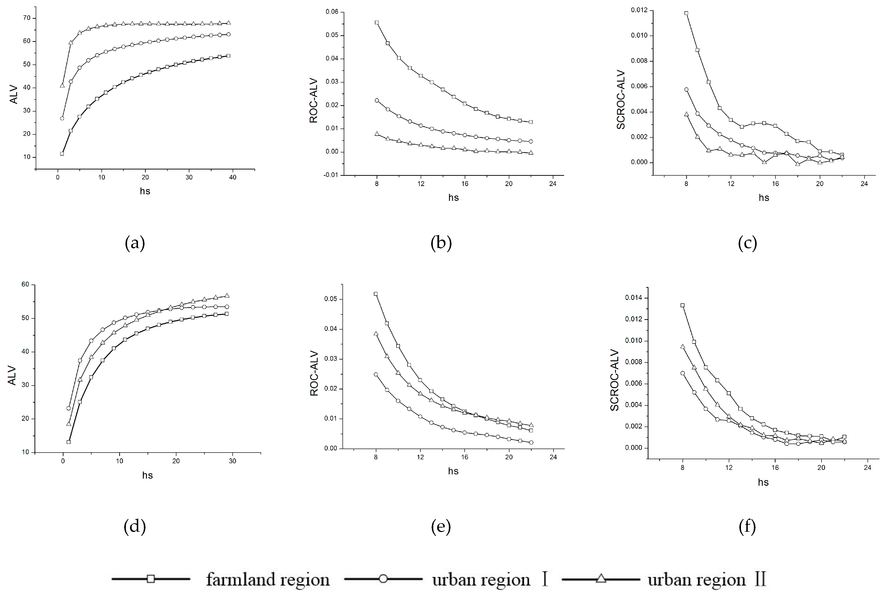
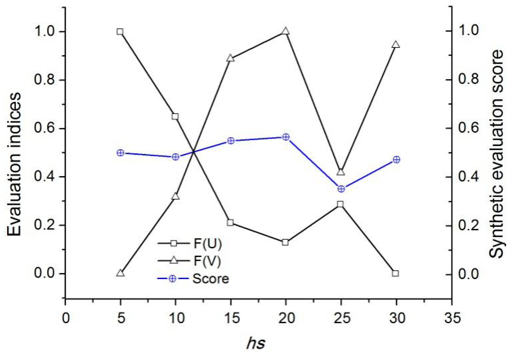
• Pre-segmentation scale estimation based on spatial statistics. Contrasted with the two methods mentioned above, this method only needs spatial statistical features. Ming et al. generalized the commonly used segmentation scale parameters into three general aspects: spatial parameter h_s, attribute/spectral parameter h_r, and area parameter M [47]. Meanwhile, Ming et al. used the average local variance (ALV) [48] or the semivariogram [49] to estimate the optimal h_s, h_r, and M. Because this method is completely data-driven, it can reduce the experimental steps and improve the efficiency without the tedious multiple scale segmentation.

In conclusion, considering the regional division and scale selection, this paper presents a stratified scale pre-estimation method to extract farmland from VHR images, meeting the need of precision agriculture and modern agriculture for farmland fine geometric information.

2. Materials and Methods

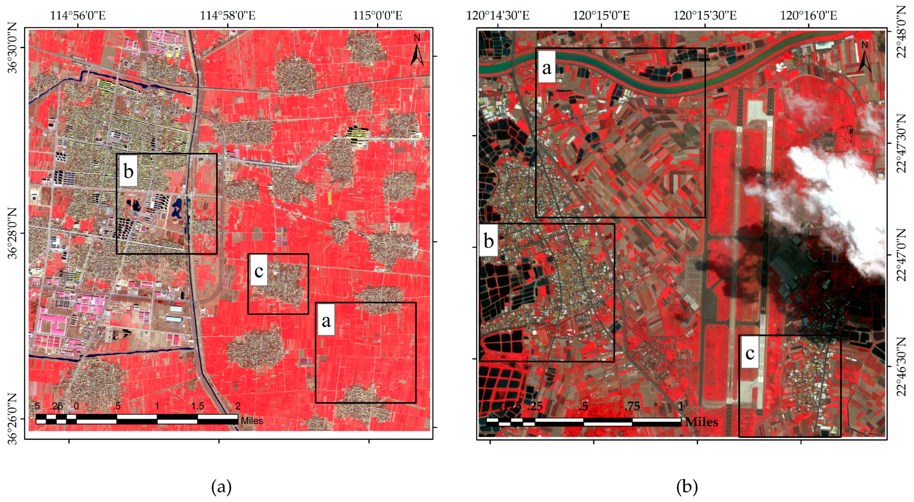
2.1. Study Area and Experimental Data

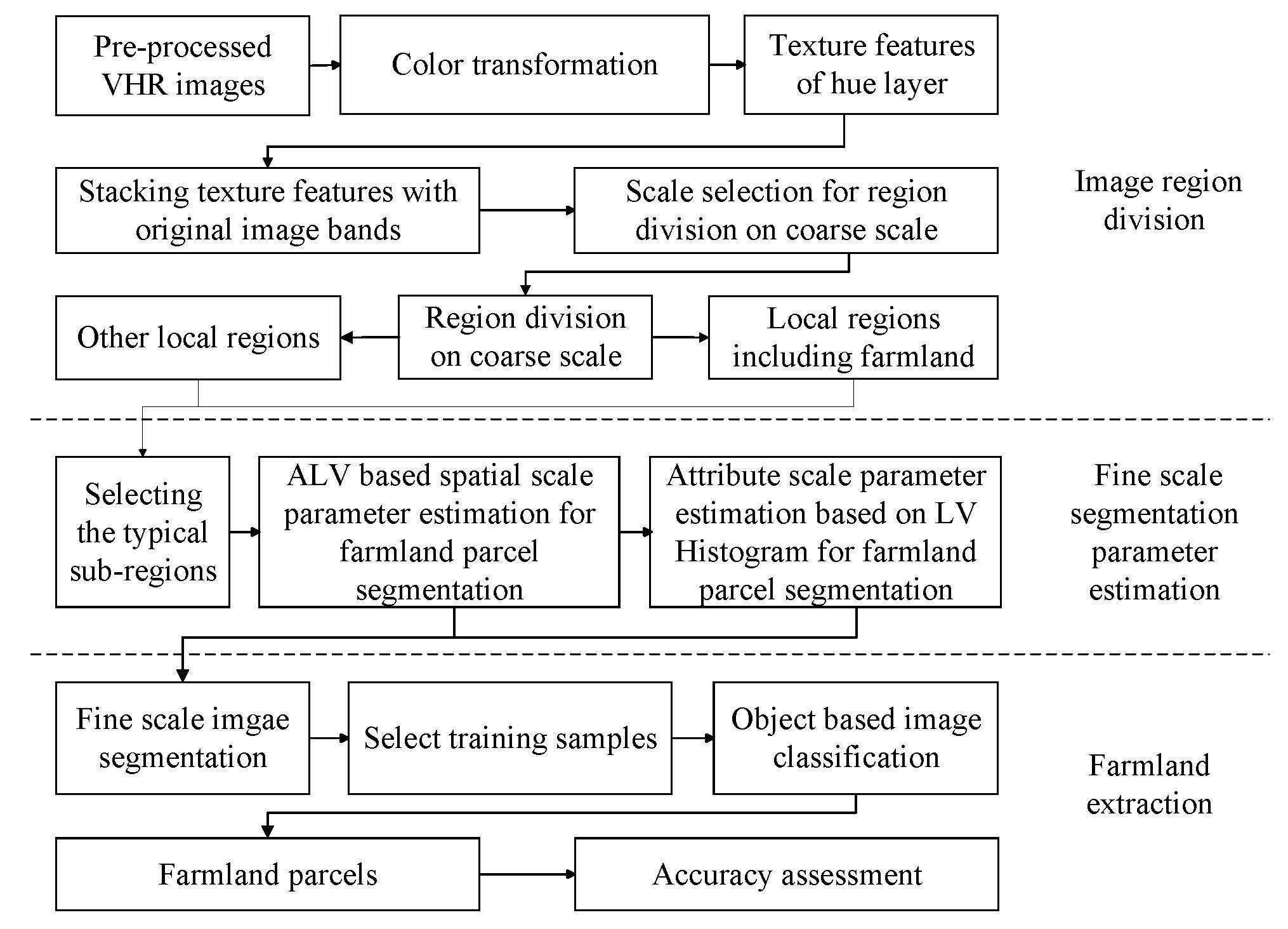
The study areas are located in the countryside of Handan, Hebei province and Gaoxiong, Taiwan province, China. For the mean-shift segmentation experiment, this study uses multispectral images acquired by GF-2 on 25 February 2017 and the image size is 2000 × 2000 pixels, with a spatial resolution of 4m. Four bands of the multispectral image were studied, namely, blue (0.45–0.52 μm), green (0.52–0.59 μm), red (0.63–0.69 μm), and near-infrared (NIR, 0.77–0.89 μm), which have similar spectral ranges to the Quickbird multispectral image.

For the multi-resolution segmentation experiment, this study uses multispectral images acquired by Quickbird (2.8m spatial resolution) on 3 July, and the image size is 1200 × 1200 pixels. Figure 1 shows the false color composition of the study area.

2.2. Methods

This paper presents a stratified object-based farmland extraction method based on image region division on a rough scale and scale parameter pre-estimation within local regions. Figure 2 shows the workflow of the proposed method.

In the first (image region division) step, the paper considers both spectrum and texture information of VHR images and employs the ESP tool to select coarse scale parameters in a multi-resolution segmentation algorithm. After that, it can obtain some local regions, which includes farmland covered regions. For the second (fine scale segmentation parameters estimation) step, this paper uses an ALV and LV histogram to estimate the spatial scale parameter and attribute scale parameter, respectively. However, because the local images have an irregular shape, directly gathering statistics on them will cause errors. Thus, this study selects the typical sub-regions of the image based on regional division before scale estimation. For the last step, in order to verify that the presented method is suitable for multiple data and different segmentation algorithms, the paper synthetically applies GF-2, Quickbird image, mean-shift, and multi-resolution segmentation algorithms to extract farmland. Uniformly, this paper uses a rule-based classifier in eCognition software. More details on each step are provided below.

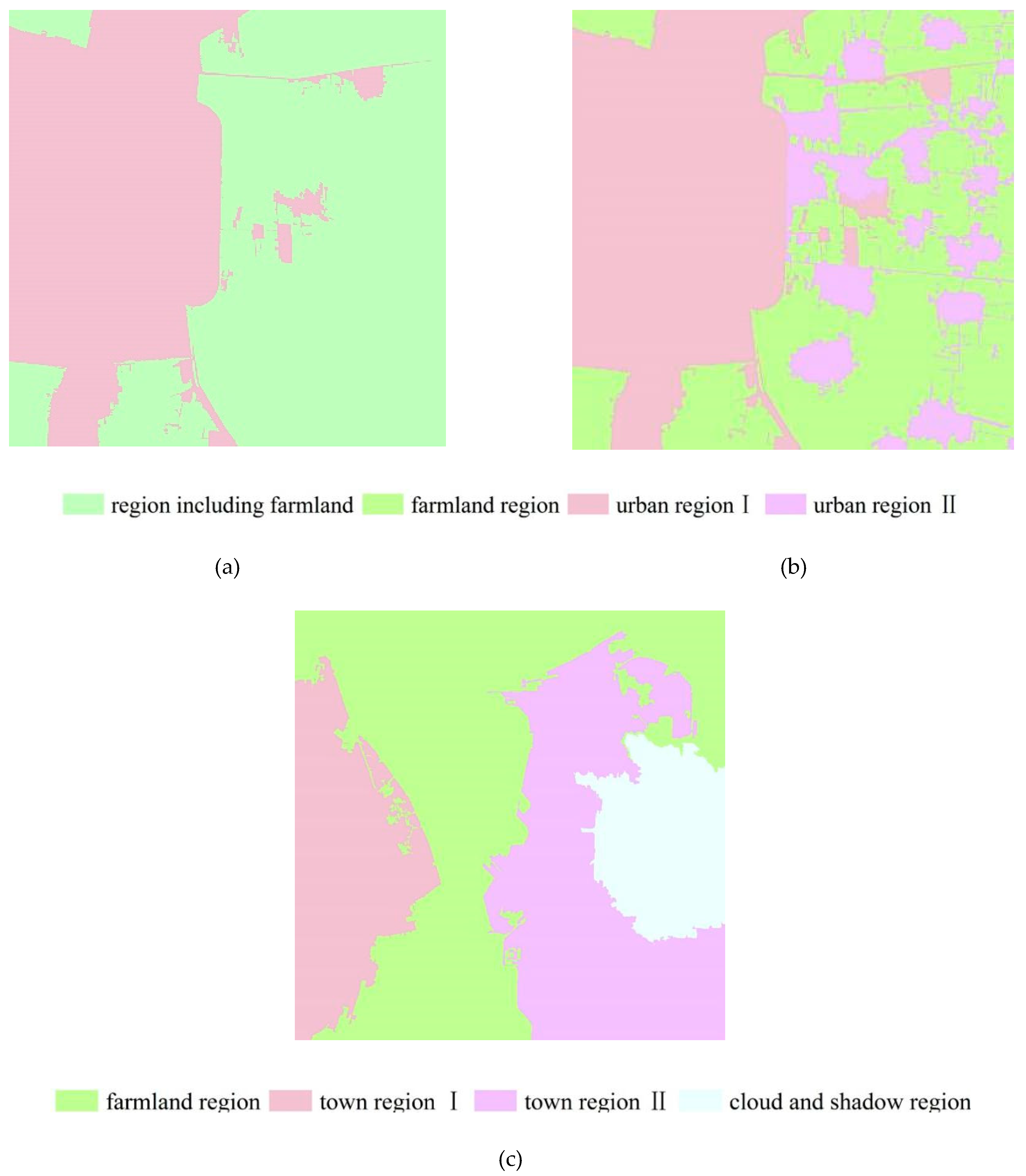
2.2.1. Region Division on Rough Scale

Tobler proposed that the shorter the distance between two objects is, the more related they will be [50]. In other words, similar natural objects always cluster in the same local region with similar sizes. Thus, dividing the VHR images and extracting farmland in local regions can improve the suitability and accuracy of scale.

● Color transformation

In order to enhance the visual effect of multi-spectral images, researchers use different combinations of RGB colors to show different objects. However, it is necessary to quantitate colors because of the value difference in RGB color space among similar colors. Compared with other color representation methods, the colors in HSV color space are closer compared to human vision [51]. It describes color with hue, saturation, and intensity. The hue layer contains digital number values of the original images and objects with a similar color that have similarities in the hue layer.

● Texture features extraction

Textures are local features of remote sensing images, and the first and second order of spatial statistic features are usually used as textural measurements. Compared with the first order texture matrix, the second order matrix considers the relationship between the referenced pixel and its neighbor pixels. Grey Level Co-occurrence Matrix (GLCM) is a matrix in which elements are the amount of the spatial combination times (i.e., the referenced pixel and its neighbor pixels co-occur in different statistic window sizes and displacements) [52,53]. Normalized GLCM (NGLCM) can represent the frequency of gray value combinations, and it is the frequency of each combination divided by the total frequency:

$$P_{i,j}=\frac{V_{i,j}}{{\displaystyle \sum _{i,j=0}^{N-1}{V}_{i,j}}}$$

(1)

where i, j (i, j = 0, 1, 2 … N − 1) means the image gray level and N means the image grayscale. P_i,j and V_i,j stand for the NGLCM and the GLCM elements, respectively. These notations have the same meaning as the following Formula (2)–(4).

Most texture features are the weighted average of NGLCM elements, which emphasizes the importance of different values in NGLCM. There are different kinds of indexes to describe the objects’ texture features, such as the mean, entropy, homogeneity, variance, contrast, dissimilarity, correlation, second moment, and so on [54]. Considering the different importance of these textural features, this paper uses mean, entropy, and homogeneity as the typical textural features for regional division.

The mean reflects the regulation of remote sensing images’ texture. The mean of GLCM is the expectation of the discrete random variables, which can be computed by Formula (2). The more regular the image texture, the larger the mean value will be [55].

$$u_i={\displaystyle \sum _{i,j=0}^{N-1}i{P}_{i,j}}\hspace{1em}{u}_j={\displaystyle \sum _{i,j=0}^{N-1}j{P}_{i,j}}$$

(2)

where u_i and u_j represent the mean of the referenced and neighbor pixels in NGLCM, respectively. Due to the symmetry of NGLCM, u_i and u_j are equal in value.

Entropy represents the complexity or heterogeneity of images’ texture. If the textures are complicated and the neighbor values have a great difference, the values of entropy will be larger. Entropy (Ent) can be calculated as below:

$$Ent={\displaystyle \sum _{i,j=0}^{N-1}{P}_{i,j}}(-\ln P_{i,j})$$

(3)

The value of homogeneity, which represents the homogeneity of different local regions, will decline when the typical objects change sharply. The value of local regions dominated by a single type of object stabilizes or fluctuates in the vicinity of a certain number. However, in practice, the value greatly fluctuates at local regions with mixed type objects, which provides the theoretical basis for scale stratified processing. According to this, the whole image can be divided into different regions based on homogeneity feature on a rough scale. Homogeneity (Hom) can be calculated as below:

$$Hom={\displaystyle \sum _{i,j=0}^{N-1}\frac{P_{i,j}}{1+{(i-j)}^2}}$$

(4)

In conclusion, this region division method transforms an image from RGB color space to HSV by color transformation, and then extracts hue layer texture features with GLCM. Finally, three textural features, the mean, entropy, and homogeneity, are used to divide the image into several local regions with high homogeneity on a rough scale. All of the processes mentioned above can be achieved in ENVI software.

● Scale selection for region division

Coarse scale and fine scale are a kind of scale nested structure, and can be expressed by a variation function from the view of spatial statistics. Ming et al. pointed out that the ALVariogram is approximately equivalent to the synthetic variogram in the condition of global traversal of the image [48]. Drǎguţ et al. proposed an estimation scale parameter (ESP) method, which is a local variance (LV) method based on post-segmentation evaluation [37]. Thus, this paper uses ESP to divide images on a coarse scale.

The ESP tool by Drǎguţ et al. built a model on the idea of the LV of object heterogeneity within a scene. It automatically segments the image with given scale parameters, and calculates the LV of the objects because each object level is acquired through segmentation. The graphics of LV and its rate of change (ROC) are used to evaluate the appropriate scale parameters [37] (i.e., the peak of the ROC curve indicates the optimal scale parameter). ROC can be calculated by Formula (5):

$$ROC=\left[\frac{L-(L-1)}{L-1}\right]\times 100$$

(5)

where L = LV at the target level and L − 1 = LV at the next lower level.

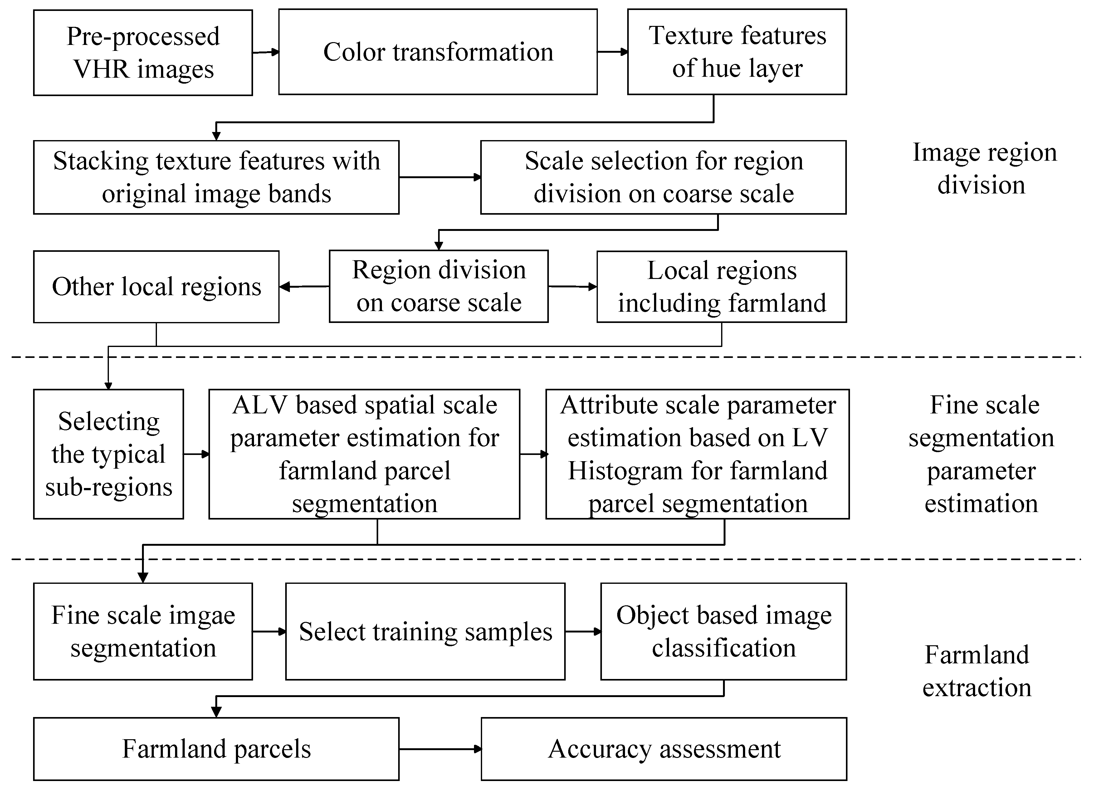
2.2.2. Scale Parameters Pre-Estimation in Local Regions

Scale is a widely used term. In general scientific research, scale mainly refers to the range or degree of detail in research [56]. Because the basic unit of object-based image analysis (OBIA) is image object, the scale in OBIA simply means the scale of image object, which is the size of image object in the spatial domain. Ming et al. pointed out that from the view of the algorithm, the scale selection in OBIA corresponds to the scale parameters selection in the multi-scale segmentation algorithm because the image object is obtained by image segmentation [57,58]. Based on the spatial and attribute features of spatial data, scale parameters are summarized as spatial scale segmentation parameter h_s (spatial distance between classes or range of spatial correlations), attribute scale segmentation parameter h_r (attribute difference between classes), and area parameter M (the area or pixel number of the minimum meaningful object).

The essence of the scale problem remains as spatial autocorrelation or scale dependent in spatial statistics, and the appropriate scale is a critical point which can exactly reflect the existence of spatial correlation between ground objects. According to Ming et al.’s research [47], this paper uses the scale pre-estimation method to select scale parameters. The essence of the method is based on the statistic estimation of global or local features. First, the average local variance (ALV) of the image is calculated. Formula (6) shows the relation between h_s and window size (w). Then, the first-order rate of change in ALV (ROC-ALV) and the second-order change in ALV (SCROC-ALV) are used to assess the dynamics of ALV along h_s (7-8). The related formulas for calculating ROC-ALV and SCROC-ALV are as follows:

$$w=2\times h_s+1$$

(6)

$${[ROC-ALV]}_i=\frac{AL{V}_i-AL{V}_{i-1}}{AL{V}_{i-1}}$$

(7)

$${[SCROC-ALV]}_i={[ROC-ALV]}_{i-1}-{[ROC-ALV]}_i$$

(8)

where i stands for the target level and i − 1 stands for the next target level. [ROC-ALV]_i is the rate of change in ALV at level h_s, and the value of [ROC-ALV]_i is usually between [0,1]. [SCROC-ALV]_i is the change of [ROC-ALV]_i, and the value of [SCROC-ALV]_i is also usually between [0,1]. Most of the [SCROC-ALV]_i values are small fractions.

The thresholds of ROC-ALV and SCROC-ALV are respectively set as 0.01 and 0.001, which means the optimal h_s is determined by the window size w when the value of [ROC-ALV]_i is less than 0.01 and [SCROC-ALV]_i is less than 0.001 for the first time. Based on the estimated h_s, the LV histogram’s first peak is used to assist in estimating the value of h_r. In order to ensure that the segmentation results are entirely determined by h_s and h_r, here, M is set as 0.

Because the scale parameters pre-estimation method is applicable to almost all image segmentation methods, this paper takes the mean-shift segmentation and multi-resolution segmentation as examples to demonstrate the feasibility of the proposed workflow for farmland extraction from VHR remote sensing images.

● Mean-shift segmentation

The mean-shift segmentation algorithm, a clustering method [59], incorporates the spatial information into the feature space representation. This algorithm does not require a priori knowledge of the number of clusters, and it can shift the points in the feature space to the local maxima of the density function by effective iterations [60,61]. Thus, the mean-shift segmentation algorithm is widely used and has advantages for farmland extraction [62,63]. In mean-shift-based multi-scale segmentation, there are three scale parameters: spatial bandwidth, attribute bandwidth, and merging threshold [64,65,66]. The three scale parameters exactly correspond to the three scale parameters (h_s,h_r,M) presented in this paper. Therefore, the scale parameters of the pre-estimation approach presented in this paper can also be applied to estimate the appropriate scale parameters of mean-shift segmentation.

● Multi-resolution segmentation

Multi-resolution segmentation (MRS) is a bottom-up region-growing technique [67], which is one of the most commonly used image segmentation algorithms [68]. It starts with one-pixel objects and merges similar neighboring objects together in subsequent steps until a heterogeneity threshold, set by a scale parameter (SP), is reached [69]. Other user-defined segmentation parameters include band weight, color/shape weight (w1), and smoothness/compactness weight (w2). SP, an important parameter of the multi-resolution segmentation algorithm, means the upper limit for a permitted change of heterogeneity throughout the segmentation process and directly determines the average image object size [70]. This paper uses the algorithm provided by eCognition software in image segmentation. When the shape heterogeneity is set as 0, the parameter SP is uniquely determined by spectral heterogeneity, and in this condition, the scale parameter SP corresponds to h_r², the square of spectral differences [71]. The lager the SP value, the bigger the image object sizes will be.

3. Experiments

In order to verify the feasibility of the proposed method, this paper used GF-2 and Quickbird images as experimental data. Mean-shift and multi-resolution segmentation algorithms were used to segment two experimental data, respectively. The overall accuracy (OA) and farmland extraction accuracy (FEA) were applied to evaluate the accuracy of farmland extraction. FEA refers to the user’s accuracy of farmland (e.g., high vegetation covered farmland and low vegetation covered farmland), which means an omission error [16]. In order to prove the validity of proposed method, we compared the farmland extraction results of the proposed stratified scale pre-estimation based method with those of the undivided method by the original image.

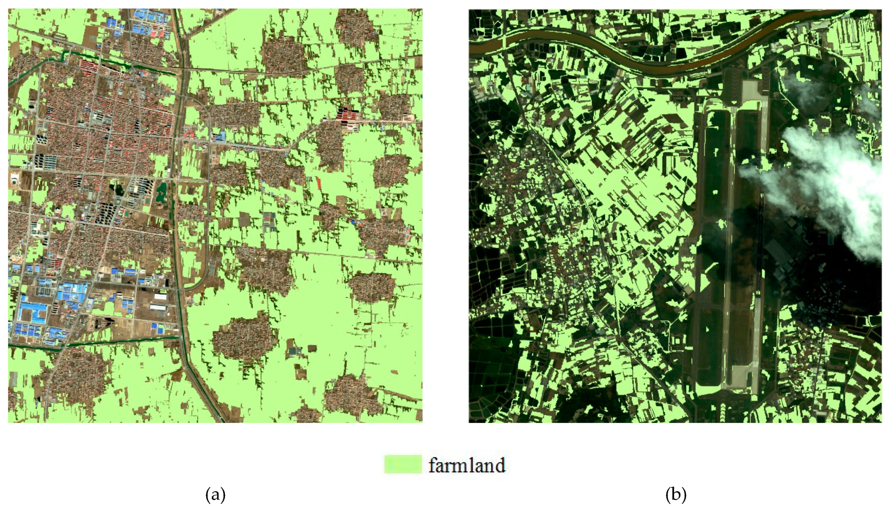
3.1. Experiments of Farmland Extraction Based on Stratified Scale Pre-Estimation

For the GF-2 image, color space (near infrared, red, and green bands) was firstly converted from RGB into HSV. Second, texture features of the hue layer were calculated using a 3 × 3 window from the upper left to the lower right. Third, layers of hue, mean, entropy, homogeneity, and original image bands were stacked into a new image as the data source of regional division. Before the segmentation of regional division, the ESP tool was used to estimate the optimal scale parameter and the estimation results are shown in Figure 3a, according to which 800 was selected as the optimal parameter for the first time region partition. Fourth, the generated image was segmented by using the multi-resolution segmentation method, in which the weight of hue, mean, and homogeneity was set as 2, while the weight of other layers was set as 1. Scale parameter, shape index, and compactness index were set as 800, 0.1, and 0.5, respectively. After that, an urban region and a mixed region which includes farmland were obtained as shown in Figure 4a. Next, we used the ESP tool to estimate the second regional division parameter, and 280 was selected as the optimal scale parameter, as shown in Figure 3b. The mixed region was segmented by the multi-resolution segmentation method with the estimated second regional division scale parameter, and the shape index and compactness index were set as 0.1 and 0.5, respectively. Finally, by combining the two segmentation results and merging the small broken parts, the GF-2 image was divided into three local regions called the farmland region, urban region I, and urban region II, as shown in Figure 4b.

For the Quickbird image, the processing is similar to the GF-2 experiment. Differently, the optimal scale parameter estimated by the ESP tool is 700. As shown in Figure 4c, the Quickbird image was segmented into four local regions: cloud and shadow region, farmland region, urban region I, and urban region II.

Before scale parameter estimation in local regions and image segmentation, the depth of the image was reduced to 8 bits, which can not only ensure the consistency of results, but also reduce the calculation quantity of the experiment. In order to avoid the statistic error, this paper estimated scale parameters within a typical sub-region instead of an irregular original local image, as shown in Figure 1. The estimation of h_s and h_r is shown in Figure 5 and Figure 6.

Then, local images were segmented with the estimated parameters listed in

Table 1. Estimated scale parameters.

Region	GF-2 Image Experiment		Quickbird Image Experiment
	Estimated hs	Estimated hr	Estimated hs	Estimated hr	Estimated SP
farmland region	20	5	17	6	36
urban region I	15	7	14	7	49
urban region II	10	8	15	7	49

. For the GF-2 image, in order to extract farmland, four categories, including high vegetation covered farmland, low vegetation covered farmland, bare land, and construction land, were determined by visual interpretation. For the Quickbird experiment, the image was classified into five categories, including high vegetation covered farmland, low vegetation covered farmland, water, vegetation except farmland, and construction land. The numbers of training and testing samples are shown in

Table 2. Descriptions of land-cover types and sample amounts.

Class	GF-2 Image Experiment		Quickbird Image Experiment
	Training Sample Amounts	Testing Sample Amounts	Training Sample Amounts	Testing Sample Amounts
Low	27	54	42	79
High	23	311	18	29
Con	25	375	50	103
Bare	30	97
Water			10	20
Veg			56	101
Total	105	837	176	332

Low refers to low vegetation covered farmland, High refers to high vegetation covered farmland, Con refers to construction land, Bare refers to bare land, and Veg refers to vegetation except farmland.

. Local regional classified results were merged into a complete image, in which the confusion matrix is accumulated by each regional results’ confusion matrix in the corresponding position. Finally, as shown in

Table 3. OA and FEA of classification results.

Image	GF-2 Image Experiment		Quickbird Image Experiment
	OA	FEA	OA	FEA
farmland region	0.8113	0.9391	0.6977	0.8633
urban region I	0.6603	0.8182	0.8364	0.2069
urban region II	0.6344	0.6667	0.8361	0.4756
merged image	0.7238	0.9154	0.7693	0.7326

, the OA and FEA of the classification results were recorded.

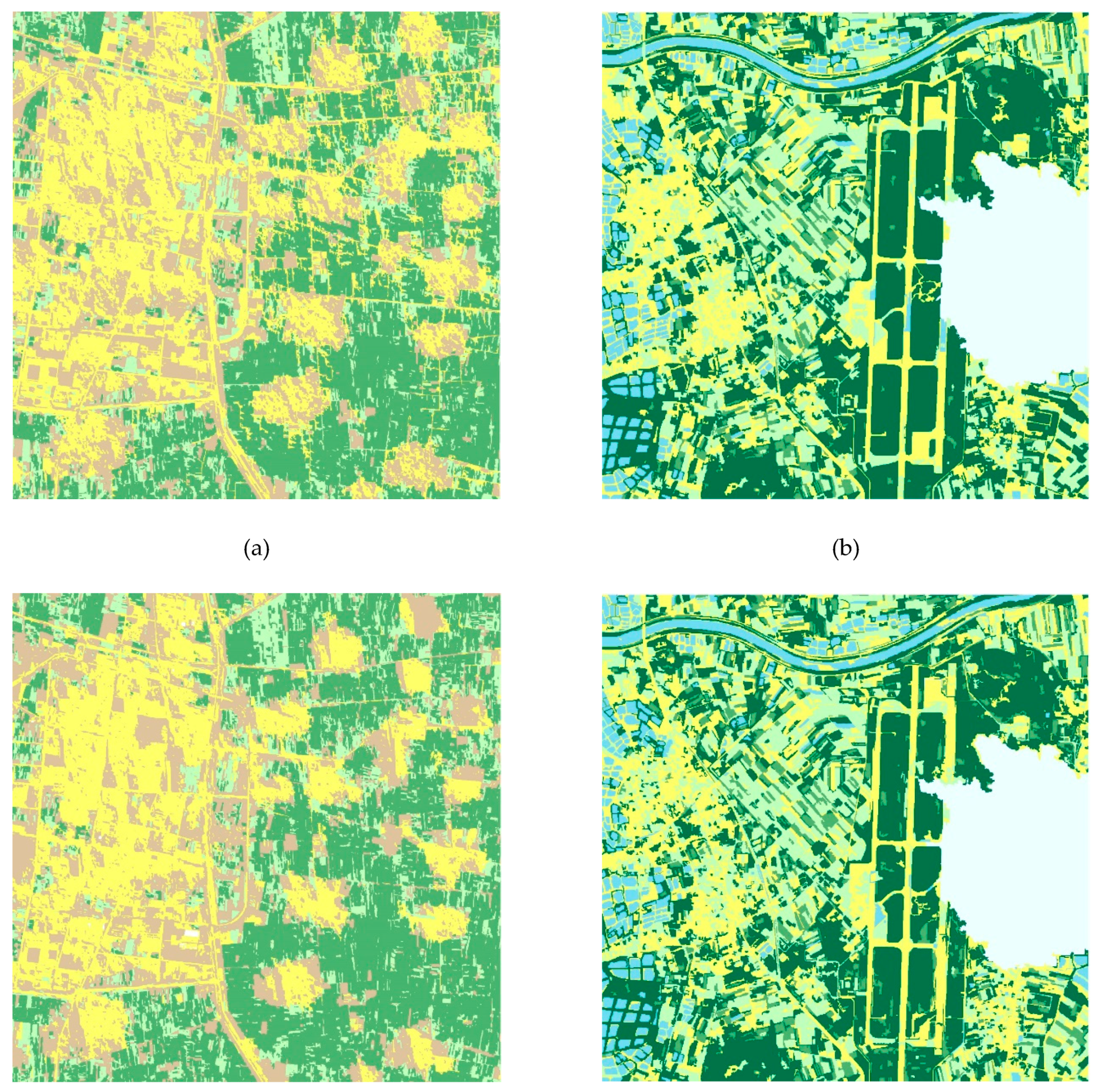
3.2. Experimental Results

The final farmland extraction results, which contain two categories (high vegetation covered farmland and low vegetation covered farmland), are demonstrated in Figure 7. Table 3 shows the OA and FEA of classification results and the classification images are shown in Figure 8a,b. For the GF-2 image, the OA and FEA of the three local regions merged image are 0.7238 and 0.9154, respectively. Furthermore, for the Quickbird image, the OA is 0.7693 and the FEA is 0.7326.

3.3. Contrast Experiments

In order to verify the validity of the proposed method, we segmented and classified the original image without using stratified processing (using the estimated optimal parameters that are suitable for extracting the farmland for the whole image). The comparison classification results image of the two experiments without having been stratified are shown in Figure 8c,d.

Table 4. OA and FEA of two experiments.

Image	OA		FEA
	Stratified Method	Original Image Without Stratified Processing	Stratified Method	Original Image Without Stratified Processing
GF-2	0.7238	0.6984	0.9154	0.9075
Quickbird	0.7693	0.7187	0.7326	0.6473

shows the OA and FEA of the merged image by the proposed stratified method and original image without stratified processing. The OA is improved by 3.64% and 7.04%, respectively, in the two experiments. According to the two experimental results mentioned above, it is proved that the proposed stratified scale pre-estimated method can extract farmland qualitatively and quantitatively and it has practical significance in large extent remote sensing geo-applications ascribed to regional division.

4. Discussion

4.1. Effectiveness of Scale Parameters Estimation

In order to evaluate the proposed scale parameters estimation method, this paper utilized the synthetic evaluation model (SEM) to test the optimal scale parameters [72]. SEM is based on homogeneity within the segmentation parcels (F(U)) and the heterogeneity between the parcels (F(V)). The synthetic evaluation score (Score) is calculated by Formula (9):

$$Score=w\times F(U)+(1-w)\times F(V)$$

(9)

where w is the weight of the homogeneity index.

For more details about SEM, please refer to Ming et al. [49]. This paper used the sub-region of the farmland region in the GF-2 image (shown in Figure 1a) and the mean-shift segmentation algorithm as an example to verify the accuracy of the proposed method.

To reduce the computation of verification, the evaluation of the segmentation results is based on h_s from 5 to 30, with a step of 5. The h_r and M are set as 5 and 0, respectively. The evaluation results are shown in Figure 9, where w is set as 0.5.

Figure 9 clearly shows that Score has the maximum value when h_s is 20, and it is the same as the estimation result generated by the proposed method. This result means that the scale parameters pre-estimation method could obtain the optimal scale parameters in a sense.

4.2. Influence Factors of Farmland Extraction Accuracy

A small amount of mis-classification or missed-extraction of farmland parcels still exists in the experiment. The influence factors of FEA can be considered from two aspects based on the regional division. Firstly, spectral similarity between high vegetation covered farmland and woodland (vegetation except farmland) is the main factor that causes mis-classification in the farmland region. For example, in the Quickbird image-based experiment, the vegetation located in the middle of the image is mis-classified as farmland. Secondly, farmland in the urban region is not the dominant object and the low vegetation covered farmland is often confused with construction land. The category confusion degrades the FEA, which can be presented by

Table 5. Urban region I confusion matrix of Quickbird experiment.

	Water	Con	Veg	High	Low	Sum
Water	26	2	0	0	0	28
Con	0	100	0	0	0	100
Veg	0	10	47	0	0	57
High	0	0	0	0	0	0
Low	0	23	0	0	6	29
sum	26	135	47	0	6	214

Con refers to construction land, Veg refers to vegetation except farmland, High refers to high vegetation covered farmland, and Low refers to low vegetation covered farmland.

.

The FEA values of urban region I and II in the Quickbird image are lower. However, compared with the original image without stratified processing, the FEA is still improved by 13.18% when using stratified processing. This indicates that the proposed stratified processing method is able to guarantee the thematic information extraction accuracy.

5. Conclusions

Regional processing and stratified processing are the main and classical strategies in geographical analysis. Based on scale stratified processing, this paper presents an object-based farmland extraction method. The main processes include: transforming the image from RGB color space to HSV, calculating the texture features of the hue layer, dividing the image into local regions on a coarse scale by using local variance evaluation, segmenting the image by estimated scale parameters on a fine scale, and farmland extraction by object-based classification. The superiorities of this proposed method are as follows:

• Regional division on a coarse scale can extract the farmland region on a rough scale, which not only improves the efficiency of farmland extraction, but also ensures the method’s universality;
• Pre-segmentation scale estimation based on spatial statistics can avoid under and over segmentation to a certain extent. Meanwhile, the estimation accuracy is guaranteed by the SEM method. Furthermore, it ensures the accuracy of farmland extraction;
• Theoretically, this proposed stratified processing method can be extended to extracting other thematic information which statistically satisfies the hypothesis of the second order stationary. In other words, the proposed stratified farmland extraction method is more suitable for extracting thematic information with a statistically uniform size from the images covered by a complex landscape.

Meanwhile, this proposed method also requires further improvement in future research. The accuracy of segmentation and classification is limited in the region where objects are complex. In future research, more efforts should be made to refine the categories, optimize the selection of training samples, and improve the classifiers in order to further improve the farmland extraction performance. In recent years, deep learning, semantic segmentation, and image scene classification methods have been proposed [73,74,75,76,77], and these concepts could be theoretically involved in stratified region division. In addition, there is an urgent need to develop image processing parallelization of different local images to further improve cropland extraction efficiency in future research.

References

1. Thenkabail, P.S. Global croplands and their importance for water and food security in the twenty-first century: Towards an ever green revolution that combines a second green revolution with a blue revolution. Remote Sens. 2010, 2, 2305–2312. [Google Scholar] [CrossRef]
2. Appeaning Addo, K. Urban and peri-urban agriculture in developing countries studied using remote sensing and in situ methods. Remote Sens. 2010, 2, 497–513. [Google Scholar] [CrossRef]
3. Li, Q.; Wang, C.; Zhang, B.; Lu, L. Object-based crop classification with landsat-modis enhanced time-series data. Remote Sens. 2015, 7, 16091–16107. [Google Scholar] [CrossRef]
4. Dhaka, S.; Shankar, H.; Roy, P. Irs p6 liss-iv image classification using simple, fuzzy logic and artificial neural network techniques: A comparison study. Int. J. Tech. Res. Sci. (IJTRS) 2016, 1. Available online: https://www.google.com.sg/url?sa=t&rct=j&q=&esrc=s&source=web&cd=2&ved=2ahUKEwiAivGqjeDfAhVFZt4KHUZ_BR0QFjABegQICRAB&url=http%3A%2F%2Fijtrs.com%2Fuploaded_paper%2FIRS%2520P6%2520LISS-IV%2520Image%2520Classification%2520using%2520Simple%2C%2520Fuzzy%2520%2520Logic%2520and%2520%2520Artificial%2520Neural%2520Network%2520Techniques%2520A%2520Comparison%2520Study%25201.pdf&usg=AOvVaw0JzyZUWdbKKeg3e1zIymFY (accessed on 7 January 2019).
5. Lu, L.; Yanlin, H.; Di, L.; Hang, D. A new spatial attraction model for improving subpixel land cover classification. Remote Sens. 2017, 9, 360. [Google Scholar] [CrossRef]
6. García-Pedrero, A.; Gonzalo-Martín, C.; Lillo-Saavedra, M. A machine learning approach for agricultural parcel delineation through agglomerative segmentation. Int. J. Remote Sens. 2017, 38, 1809–1819. [Google Scholar] [CrossRef]
7. Park, S.; Im, J.; Park, S.; Yoo, C.; Han, H.; Rhee, J. Classification and mapping of paddy rice by combining landsat and sar time series data. Remote Sens. 2018, 10, 447. [Google Scholar] [CrossRef]
8. Khosravi, I.; Safari, A.; Homayouni, S. Msmd: Maximum separability and minimum dependency feature selection for cropland classification from optical and radar data. Int. J. Remote Sens. 2018, 39, 1–18. [Google Scholar] [CrossRef]
9. Barbedo, J.G.A. A Review on the Automatic Segmentation and Classification of Agricultural Areas in Remotely Sensed Images. Available online: https://www.researchgate.net/publication/328073552_A_Review_on_the_Automatic_Segmentation_and_Classification_of_Agricultural_Areas_in_Remotely_Sensed_Images (accessed on 7 January 2019).
10. Thenkabail, P.S.; Biradar, C.M.; Noojipady, P.; Dheeravath, V.; Li, Y.; Velpuri, M.; Gumma, M.; Gangalakunta, O.R.P.; Turral, H.; Cai, X.; et al. Global irrigated area map (giam), derived from remote sensing, for the end of the last millennium. Int. J. Remote Sens. 2009, 30, 3679–3733. [Google Scholar] [CrossRef]
11. Thenkabail, P.S.; Lyon, J.G.; Turral, H.; Biradar, C.M. Remote Sensing of Global Croplands for Food Securit; CRC Press: Boca Raton, FL, USA, 2009; pp. 336–338. [Google Scholar]
12. Thenkabail, P.S.; Knox, J.W.; Ozdogan, M.; Gumma, M.K.; Congalton, R.G.; Wu, Z.; Milesi, C.; Finkral, A.; Marshall, M.; Mariotto, I.; et al. Assessing future risks to agricultural productivity, water resources and food security: How can remote sensing help? Photogramm. Eng. Remote Sens. 2012, 78, 773–782. [Google Scholar]
13. Thenkabail, P.S.; Wu, Z. An automated cropland classification algorithm (acca) for tajikistan by combining landsat, modis, and secondary data. Remote Sens. 2012, 4, 2890–2918. [Google Scholar] [CrossRef]
14. Chen, J.; Deng, M.; Xiao, P.; Yang, M.; Mei, X. Rough set theory based object-oriented classification of high resolution remotely sensed imagery. Int. J. Remote Sens. 2010, 14, 1139–1155. [Google Scholar]
15. Ma, L.; Li, M.; Ma, X.; Cheng, L.; Du, P.; Liu, Y. A review of supervised object-based land-cover image classification. Isprs J. Photogramm. Remote Sens. 2017, 130, 277–293. [Google Scholar] [CrossRef]
16. Lu, L.; Tao, Y.; Di, L. Object-based plastic-mulched landcover extraction using integrated sentinel-1 and sentinel-2 data. Remote Sens. 2018, 10, 1820. [Google Scholar] [CrossRef]
17. Turker, M.; Ozdarici, A. Field-based crop classification using spot4, spot5, ikonos and quickbird imagery for agricultural areas: A comparison study. Int. J Remote Sens. 2011, 32, 9735–9768. [Google Scholar] [CrossRef]
18. Chen, J.; Chen, T.; Mei, X.; Shao, Q.; Deng, M. Hilly farmland extraction from high resolution remote sensing imagery based on optimal scale selection. Trans. Chin. Soc. Agric. Eng. 2014, 30, 99–107. [Google Scholar]
19. Helmholz, P.; Rottensteiner, F.; Heipke, C. Semi-automatic verification of cropland and grassland using very high resolution mono-temporal satellite images. ISPRS J. Photogramm. Remote Sens. 2014, 97, 204–218. [Google Scholar] [CrossRef]
20. Li, M.; Ma, L.; Blaschke, T.; Cheng, L.; Tiede, D. A systematic comparison of different object-based classification techniques using high spatial resolution imagery in agricultural environments. Int. J. Appl. Earth Obs. Geoinf. 2016, 49, 87–98. [Google Scholar] [CrossRef]
21. Karydas, C.; Gewehr, S.; Iatrou, M.; Iatrou, G.; Mourelatos, S. Olive plantation mapping on a sub-tree scale with object-based image analysis of multispectral uav data; operational potential in tree stress monitoring. J. Imaging 2017, 3, 57. [Google Scholar] [CrossRef]
22. Peng, D.; Zhang, Y. Object-based change detection from satellite imagery by segmentation optimization and multi-features fusion. Int. J Remote Sens. 2017, 38, 3886–3905. [Google Scholar] [CrossRef]
23. Ming, D.; Zhang, X.; Wang, M.; Zhou, W. Cropland extraction based on obia and adaptive scale pre-estimation. Photogramm. Eng. Remote Sens. 2016, 82, 635–644. [Google Scholar] [CrossRef]
24. Ming, D.; Qiu, Y.; Zhou, W. Applying spatial statistics into remote sensing pattern recognition: With case study of cropland extraction based on geobia. Acta Geod. Et Cartogr. Sin. 2016, 45, 825–833. [Google Scholar]
25. Yi, L.; Zhang, G.; Wu, Z. A scale-synthesis method for high spatial resolution remote sensing image segmentation. IEEE Trans. Geosci. Remote Sens. 2012, 50, 4062–4070. [Google Scholar] [CrossRef]
26. Roy, P.S.; Behera, M.D.; Srivastav, S.K. Satellite remote sensing: Sensors, applications and techniques. Proc. Natl. Acad. Sci. India 2017. [Google Scholar] [CrossRef]
27. Georganos, S.; Grippa, T.; Lennert, M.; Vanhuysse, S.; Wolff, E. SPUSPO: Spatially Partitioned Unsupervised Segmentation Parameter Optimization for Efficiently Segmenting Large Heterogeneous Areas. In Proceedings of the 2017 Conference on Big Data from Space (BiDS’17), Toulouse, France, 28–30 November 2017. [Google Scholar]
28. Georganos, S.; Grippa, T.; Lennert, M.; Vanhuysse, S.; Johnson, B.; Wolff, E. Scale matters: Spatially partitioned unsupervised segmentation parameter optimization for large and heterogeneous satellite images. Remote Sens. 2018, 10, 1440. [Google Scholar] [CrossRef]
29. Zhang, X.; Du, S.; Wang, Q. Hierarchical semantic cognition for urban functional zones with vhr satellite images and poi data. Isprs J. Photogramm. Remote Sens. 2017, 132, 170–184. [Google Scholar] [CrossRef]
30. Heiden, U.; Heldens, W.; Roessner, S.; Segl, K.; Esch, T.; Mueller, A. Urban structure type characterization using hyperspectral remote sensing and height information. Landsc. Urban. Plan. 2012, 105, 361–375. [Google Scholar] [CrossRef]
31. Hu, T.; Yang, J.; Li, X.; Gong, P. Mapping urban land use by using landsat images and open social data. Remote Sens. 2016, 8, 151. [Google Scholar] [CrossRef]
32. Kavzoglu, T.; Yildiz Erdemir, M.; Tonbul, H. A region-based multi-scale approach for object-based image analysis. ISPRS Int. Arch. Photogramm. Remote Sens. Spat. Inf. Sci. 2016, XLI-B7, 2412–2447. [Google Scholar]
33. Zhou, W.; Ming, D.; Xu, L.; Bao, H.; Wang, M. Stratified object-oriented image classification based on remote sensing image scene division. J. Spectrosc. 2018, 3918954. [Google Scholar] [CrossRef]
34. Grybas, H.; Melendy, L.; Congalton, R.G. A comparison of unsupervised segmentation parameter optimization approaches using moderate- and high-resolution imagery. GISci. Remote Sens. 2017, 54, 515–533. [Google Scholar] [CrossRef]
35. Drǎguţ, L.; Csillik, O.; Eisank, C.; Tiede, D. Automated parameterisation for multi-scale image segmentation on multiple layers. ISPRS J. Photogramm. Remote Sens. 2014, 88, 119–127. [Google Scholar] [CrossRef] [Green Version]
36. Drǎguţ, L.; Eisank, C.; Strasser, T. Local variance for multi-scale analysis in geomorphometry. Geomorphology 2011, 130, 162–172. [Google Scholar] [CrossRef] [PubMed] [Green Version]
37. Drǎguţ, L.; Tiede, D.; Levick, S.R. Esp: A tool to estimate scale parameter for multiresolution image segmentation of remotely sensed data. Int. J. Geogr. Inf. Sci. 2010, 24, 859–871. [Google Scholar] [CrossRef]
38. Woodcock, C.E.; Strahler, A.H. The factor of scale in remote sensing. Remote Sens. Environ. 1987, 21, 3113–3132. [Google Scholar] [CrossRef]
39. Johnson, B.; Xie, Z. Unsupervised image segmentation evaluation and refinement using a multi-scale approach. ISPRS J. Photogramm. Remote Sens. 2011, 66, 4734–4783. [Google Scholar] [CrossRef]
40. Georganos, S.; Lennert, M.; Grippa, T.; Vanhuysse, S.; Johnson, B.; Wolff, E. Normalization in unsupervised segmentation parameter optimization: A solution based on local regression trend analysis. Remote Sens. 2018, 10, 222. [Google Scholar] [CrossRef]
41. Zhang, X.; Du, S. Learning selfhood scales for urban land cover mapping with very-high-resolution satellite images. Remote Sens. Environ. 2016, 178, 1721–1790. [Google Scholar] [CrossRef]
42. Zhang, X.; Xiao, P.; Feng, X.; Feng, L.; Ye, N. Toward evaluating multiscale segmentations of high spatial resolution remote sensing images. IEEE Trans. Geosci. Remote Sens. 2015, 53, 3694–3706. [Google Scholar] [CrossRef]
43. Clinton, N.; Holt, A.; Scarborough, J.; Yan, L.; Gong, P. Accuracy assessment measures for object-based image segmentation goodness. Photogramm. Eng. Remote Sens. 2010, 76, 2892–2899. [Google Scholar] [CrossRef]
44. Estrada, F.J.; Jepson, A.D. Benchmarking image segmentation algorithms. Int. J. Comput. Vis. 2009, 85, 1671–1681. [Google Scholar] [CrossRef]
45. Albrecht, F. Uncertainty in image interpretation as reference for accuracy assessment in object-based image analysis. In Proceedings of the Ninth International Symposium on Spatial Accuracy Assessment in Natural Resources and Environmental Sciences, Leicester, UK, 20–23 July 2010; pp. 13–16. [Google Scholar]
46. Chen, Y.; Ming, D.; Zhao, L.; Lv, B.; Zhou, K.; Qing, Y. Review on high spatial resolution remote sensing image segmentation evaluation. Photogramm. Eng. Remote Sens. 2018, 84, 629–646. [Google Scholar] [CrossRef]
47. Ming, D.; Zhou, W.; Wang, M. Scale parameter estimation based on the spatial and spectral statistics in high spatial resolution image segmentation. J. Geo-Inf. Sci. 2016, 18, 6226–6231. [Google Scholar]
48. Ming, D.; Li, J.; Wang, J.; Zhang, M. Scale parameter selection by spatial statistics for geobia: Using mean-shift based multi-scale segmentation as an example. Isprs J. Photogramm. Remote Sens. 2015, 106, 28–41. [Google Scholar] [CrossRef]
49. Ming, D.; Ci, T.; Cai, H.; Li, L.; Qiao, C.; Du, J. Semivariogram-based spatial bandwidth selection for remote sensing image segmentation with mean-shift algorithm. IEEE Geosci. Remote Sens. Lett. 2012, 9, 813–817. [Google Scholar] [CrossRef]
50. Tobler, W.R. A computer movie simulating urban growth in the detroit region. Econ. Geogr. 1970, 46, 234–240. [Google Scholar] [CrossRef]
51. Wei, C.; Tang, G.; Wang, M.; Yang, X. Processes of Remote Sens. Digital Image; Springer: Berlin, Germany, 2015. [Google Scholar]
52. Hall-Beyer, M. The GLCM tutorial. In Proceedings of the National Council on Geographic Information and Analysis Remote Sensing Core Curriculum, 2000; Available online: https://www.researchgate.net/profile/Mryka_Hall-Beyer/publication/315776784_GLCM_Texture_A_Tutorial_v_30_March_2017/links/58e3e0b10f7e9bbe9c94cc90/GLCM-Texture-A-Tutorial-v-30-March-2017.pdf (accessed on 7 January 2019).
53. Hall-Beyer, M. Practical guidelines for choosing glcm textures to use in landscape classification tasks over a range of moderate spatial scales. Int. J. Remote Sens. 2017, 38, 13121–13338. [Google Scholar] [CrossRef]
54. Haralick, R.M.; Shanmugam, K.; Dinstein, I. Textural features for image classification. IEEE Trans. Syst. ManCybern. 1973, SMC-3, 6106–6121. [Google Scholar] [CrossRef]
55. Hong, J. Gray level-gradient cooccurrence matrix texture analysis method. Acta Autom. Sin. 1984, 10, 222–225. [Google Scholar]
56. Goodchild, M.; Quattrochi, D.A. Scale in Remote Sens, and GIS; Lewis Publishers: Boca Raton, FL, USA, 1997; pp. 114–120. [Google Scholar]
57. Ming, D.; Yang, J.; Li, L.; Song, Z. Modified alv for selecting the optimal spatial resolution and its scale effect on image classification accuracy. Math. Comput. Model. 2011, 54, 1061–1068. [Google Scholar] [CrossRef]
58. Ming, D.; Zhou, W.; Xu, L.; Wang, M.; Ma, Y. Coupling relationship among scale parameter, segmentation accuracy, and classification accuracy in geobia. Photogramm. Eng. Remote Sens. 2018, 84, 6816–6893. [Google Scholar] [CrossRef]
59. Chen, R.; Zheng, C.; Wang, L.; Qin, Q. A region growing model under the framework of mrf for urban detection. Acta Geod. Et Cartogr. Sin. 2011, 40, 163. [Google Scholar]
60. Wang, L.G.; Zheng, C.; Lin, L.Y.; Chen, R.Y.; Mei, T.C. Fast segmentation algorithm of high resolution remote sensing image based on multiscale mean shift. Spectrosc. Spectr. Anal. 2011, 31, 177. [Google Scholar]
61. Wang, L.; Liu, G.; Mei, T.; Qin, Q. A segmentation algorithm for high-resolution remote sensing texture based on spectral and texture information weighting. Acta Opt. Sin. 2009, 29, 3010–3017. [Google Scholar] [CrossRef]
62. Su, T.; Li, H.; Zhang, S.; Li, Y. Image segmentation using mean shift for extracting croplands from high-resolution remote sensing imagery. Remote Sens. Lett. 2015, 6, 9529–9561. [Google Scholar] [CrossRef]
63. Su, T.; Zhang, S.; Li, H. Variable scale mean-shift based method for cropland segmentation from high spatial resolution remote sensing images. Remote Sens. Land Resour. 2017, 6, 952–961. [Google Scholar]
64. Comaniciu, D. An algorithm for data-driven bandwidth selection. IEEE Trans. Pattern Anal. Mach. Intell. 2003, 25, 2812–2888. [Google Scholar] [CrossRef]
65. Comaniciu, D.; Meer, P. Mean shift: A robust approach toward feature space analysis. IEEE Trans. Pattern Anal. Mach. Intell. 2002, 24, 603–619. [Google Scholar] [CrossRef]
66. Comaniciu, D.; Ramesh, V.; Meer, P. The variable bandwidth mean shift and data-driven scale selection. In Proceedings of the Eighth IEEE International Conference on Computer Vision ICCV 2001, Vancouver, BC, Canada, 71–74 July 2001; Volume 431, pp. 438–445. [Google Scholar]
67. Belgiu, M.; Csillik, O. Sentinel-2 cropland mapping using pixel-based and object-based time-weighted dynamic time warping analysis. Remote Sens. Environ. 2018, 204, 509–523. [Google Scholar] [CrossRef]
68. Jozdani, S.E.; Momeni, M.; Johnson, B.A.; Sattari, M. A regression modelling approach for optimizing segmentation scale parameters to extract buildings of different sizes. Int. J. Remote Sens. 2018, 39, 684–703. [Google Scholar] [CrossRef]
69. Baatz, M. Multi resolution segmentation: An optimum approach for high quality multi scale image segmentation. Beutrage Zum Agit-Symp. Salzbg. Heidelb. 2000, 2000, 12–23. [Google Scholar]
70. Cánovas-García, F.; Alonso-Sarría, F. A local approach to optimize the scale parameter in multiresolution segmentation for multispectral imagery. Geocarto Int. 2015, 30, 937–961. [Google Scholar] [CrossRef]
71. Ma, Y.; Ming, D.; Yang, H. Scale estimation of object-oriented image analysis based on spectral-spatial statistics. J. Remote Sens. 2017. [CrossRef]
72. Espindola, G.M.; Camara, G.; Reis, I.A.; Bins, L.S.; Monteiro, A.M. Parameter selection for region-growing image segmentation algorithms using spatial autocorrelation. Int. J. Remote Sens. 2006, 27, 3035–3040. [Google Scholar] [CrossRef]
73. Noh, H.; Hong, S.; Han, B. Learning deconvolution network for semantic segmentation. In Proceedings of the IEEE International Conference on Computer Vision (ICCV), Araucano Park, Las Condes, Chile, 11–18 December 2015; pp. 1520–1528. [Google Scholar]
74. Penatti, O.A.B.; Nogueira, K.; Dos Santos, J.A. Do deep features generalize from everyday objects to remote sensing and aerial scenes domains? In Proceedings of the IEEE Conference on Computer Vision and Pattern Recognition (CVPR) Workshops, Boston, MA, USA, 8–10 June 2015; pp. 44–51. [Google Scholar]
75. Ma, L.; Fu, T.; Li, M. Active learning for object-based image classification using predefined training objects. Int. J. Remote Sens. 2018, 39, 27462–27765. [Google Scholar] [CrossRef]
76. Lv, X.; Ming, D.; Chen, Y.; Wang, M. Very high resolution remote sensing image classification with seeds-cnn and scale effect analysis for superpixel cnn classification. Int. J. Remote Sens. 2018, 1–26. [Google Scholar] [CrossRef]
77. Lv, X.; Ming, D.; Lu, T.; Zhou, K.; Wang, M.; Bao, H. A new method for region-based majority voting cnns for very high resolution image classification. Remote Sens. 2018, 10, 1946. [Google Scholar] [CrossRef]
Figure 1. (a) GF-2 original image, (b) Quickbird original image. Sub-region of a-c in each image represents sampled images as farmland region, urban region I, and urban region II, respectively.
Remotesensing 11 00108 g001
Figure 2. Workflow of farmland extraction method based on stratified scale pre-estimation.
Remotesensing 11 00108 g002
Figure 3. Scale parameter estimation using ESP tool. (a) The first time estimation of GF-2 image. (b) The second time estimation of GF-2 image. (c) Estimation of Quickbird image.
Remotesensing 11 00108 g003
Figure 4. Results of regional division based on scale stratified processing. (a) The first time region division result of GF-2 image. (b) The second time region division result of GF-2 image. (c) Regional division result of Quickbird image.
Remotesensing 11 00108 g004
Figure 5. Average local variance and its relative parameters. (ac) GF-2 image experiment: (a) ALV; (b) ROC-ALV; (c) SCROC-ALV. (df) Quickbird image experiment: (d) ALV; (e) ROC-ALV; (f) SCROC-ALV.
Remotesensing 11 00108 g005
Figure 6. Histogram of local variance. (ac) GF-2 image experiment: (a) farmland region; (b) urban region I; (c) urban region II. (df) Quickbird image experiment: (d) farmland region; (e) urban region I; (f) urban region II.
Remotesensing 11 00108 g006
Figure 7. Farmland extraction results. (a) GF-2 image experiment. (b) Quickbird image experiment.
Remotesensing 11 00108 g007
Figure 8. Classification results of two images. (a) GF-2 image with stratified method. (b) Quickbird image with stratified method. (c) GF-2 original image without stratified processing. (d) Quickbird original image without stratified processing.
Remotesensing 11 00108 g008aRemotesensing 11 00108 g008b
Figure 9. Segmentation evaluations changing with hs.
Remotesensing 11 00108 g009