Walker: Continuous and Precise Navigation by Fusing GNSS and MEMS in Smartphone Chipsets for Pedestrians

Abstract

The continual miniaturization of mass-market sensors built in mobile intelligent terminals has inspired the development of accurate and continuous navigation solution for portable devices. With the release of Global Navigation Satellite System (GNSS) observations from the Android Nougat system, smartphones can provide pseudorange, Doppler, and carrier phase observations of GNSS. However, it is still a challenge to achieve the seamless positioning of consumer applications, especially in environments where GNSS signals suffer from a low signal-to-noise ratio and severe multipath. This paper introduces a dedicated android smartphone application called Walker that integrates the GNSS navigation solution and MEMS (micro-electromechanical systems) sensors to enable continuous and precise pedestrian navigation. Firstly, we introduce the generation of GNSS and MEMS observations, in addition to the architecture of Walker application. Then the core algorithm in Walker is given, including the time-differenced carrier phase improved GNSS single-point positioning and the integration of GNSS and Pedestrian Dead Reckoning (PDR). Finally, the Walker application is tested and the observations of GNSS and MEMS are assessed. The static experiment shows that, with GNSS observations, the RMS (root mean square) values of east, north, and up positioning error are 0.49 m, 0.37 m, and 1.01 m, respectively. Furthermore, the kinematic experiment verifies that the proposed method is capable of obtaining accuracy within 1–3 m for smooth and continuous navigation.

1. Introduction

In recent years, mass-market sensors have become ubiquitous in mobile intelligent terminals. GNSS chipsets, inertial measurement units (IMUs), magnetometers, and barometers are getting smaller and cheaper. The evolvement of smartphone built-in sensors facilitates the determination of a user’s positioning, space-based navigation, and time (PNT) information, which are widely recognized as important elements for global information infrastructure and are considered the basics of location-based services (LBS). Under ideal scenarios, consumer-grade GNSS receivers can reach several meters of positioning accuracy, the improvement of which will further promote the diversification of LBS [1]. However, the positioning capability will decrease in some harsh conditions, such as urban canyons or short distance tunnels, where GNSS signals suffer from a low signal-to-noise ratio and severe multipath [2,3]. Multi-GNSS receiver autonomous integrity monitoring (RAIM) can reduce the large positioning errors and achieve satisfactory positioning performance in degraded-signal scenarios [4,5]. Furthermore, pedestrian navigation systems (PNSs) are expected to provide continuous positioning and enhanced navigation performance under such cases. Based on fusing measurements of IMUs and magnetometers, the characteristics of human gait can be exploited in pedestrian dead reckoning (PDR) algorithms, which are the primary component of PNSs to continuous relative position [6,7]. A PDR system performs three main tasks: step detection, step length estimation, and heading determination [8,9]. However, the performance of a PDR system would significantly decrease with the increase in recursion time, due to sensor noise and model errors. Therefore, the absolute positioning accuracy of GNSS and the relative positioning accuracy of PDR complement each other in a smartphone, enabling the smartphone to provide continuous positioning services.

With the release of GNSS observations from the Android Nougat system, smartphones, such as Huawei P10 and Samsung S8 models, can provide pseudorange, Doppler, and carrier phase observations of GNSS systems [10]. Moreover, a new generation of mass-market chips based on dual frequency measurements is next to be commercialized [11]. These released data enable us to develop advanced algorithms to increase positioning accuracy. Using a single-frequency PPP model and an extern SBAS correction, sub-meter accuracy can be reached with android GNSS observations [12]. The decimeter positioning accuracy can also be obtained through rapid-static surveys of a real-time kinematic (RTK) model without ambiguity resolution [13,14]. Zhang et al. [15] proposed a filtering algorithm with velocity estimation of the time-differenced carrier phase (TDCP), and reached decimeter-level accuracy after convergence with static data. Some android applications utilize GNSS raw measurements already. PPP Wizlite allows precise positioning on a Nexus 5X device, and requires internet connection to obtain corrections [13]. RTMC Converter can convert android raw measurements to the RTCM format. Geo++ Rinex Logger can record android raw measurements in the Rinex file format [16]. However, this topic remains a research hotspot as researchers aim to achieve satisfactory accuracy and high availability of positioning through android smartphones, especially with GNSS observations and built-in micro-electromechanical systems (MEMS) sensors under complex pedestrian scenarios.

We developed a dedicated android application named Walker for continuous and precise pedestrian navigation by integrating GNSS and MEMS sensor observations in a smartphone. The architecture of the Walker application is introduced, including the GNSS and MEMS observations generation and synchronization as well as the positioning results in the smartphone map. Furthermore, the core algorithm of the application is given, including the improved GNSS single-point positioning with precise displacement estimation of the time-differenced carrier phase and the integration of GNSS and PDR. Finally, this application is sufficiently tested in real complex pedestrian scenarios. Both the GNSS and MEMS observations are evaluated, and some static and kinematic positioning results are provided.

2. Smartphone Pedestrian Navigation Application: Walker

In this section, the release and generation of smartphone GNSS observations is introduced. Then the concerned built-in MEMS observations are illustrated. Lastly, the structure of the Walker application is presented.

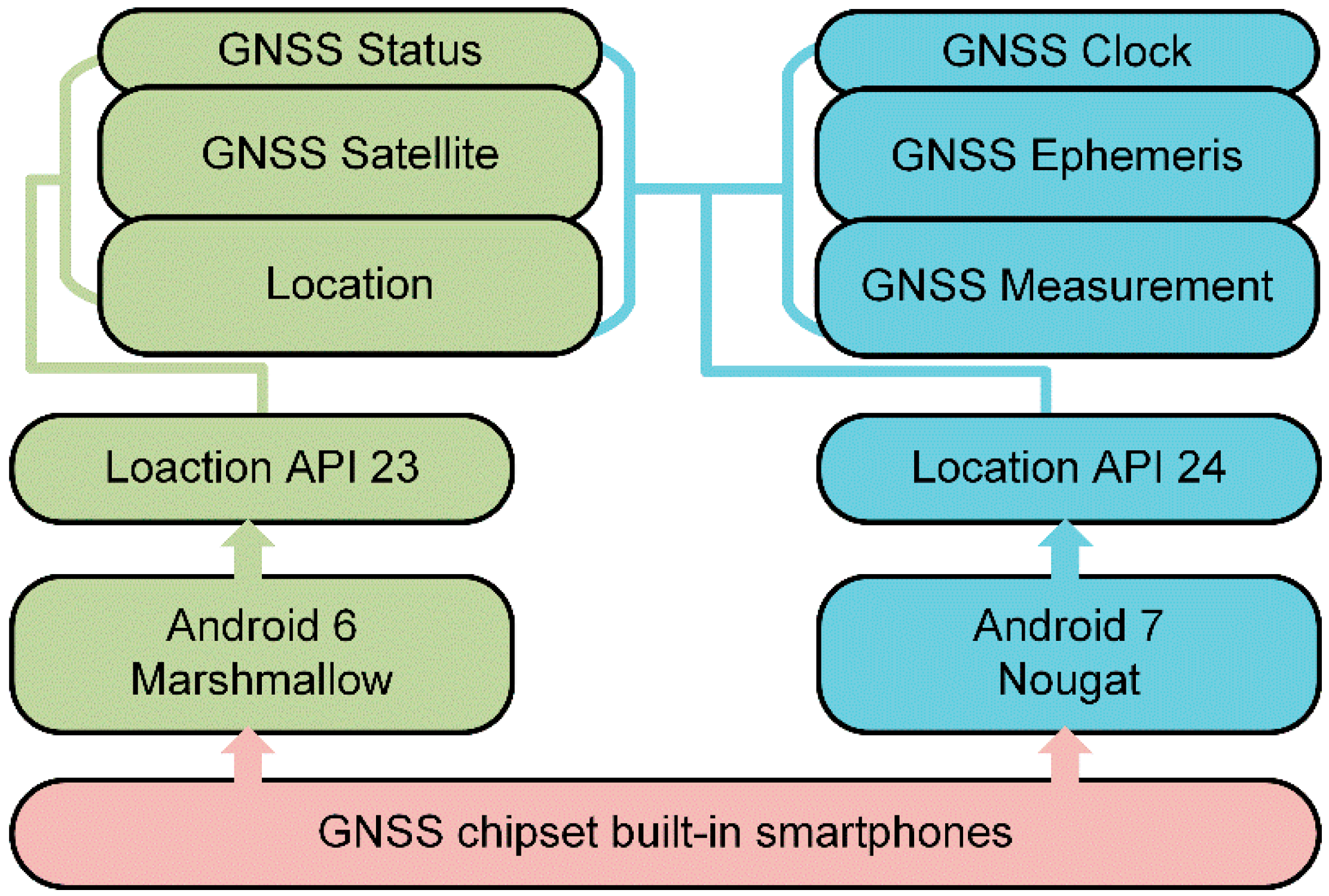
2.1. Android GNSS Observations Generation

At the Google annual I/O developer conference in May of 2016, the company reported the availability of GNSS observations in location applications programming interface (API) level 24 on the Android N (“Nougat” = version 7). Figure 1 shows the comparison of the location API structures. Until the advent of android API 23, the only data that could be obtained was GNSS satellite information, status, location, and so on, including C/N0, azimuth, elevation, PVT solutions, and satellites used in PVT. From API 24, developers have access to more data, including GNSS clock, ephemeris, and measurements. It opens the door to more advanced GNSS processing techniques, leading to improved GNSS performance.

The phase and Doppler observations are provided directly, while the pseudorange is computed with the time of signal transmitted and received as follows:

$$R=\left(T_{Rx}-T_{Tx}\right)·\frac{c}{1E9}$$

(1)

Here, R is the pseudorange, c is the speed of light, and $T_{Rx}$ and $T_{Tx}$ are the GNSS satellite time of the signal received and transmitted in nanoseconds, respectively. $T_{Rx}$ is read from the clock in the receiver, thus the same value for measurements can be provided by different satellite systems. However, $T_{Tx}$ is provided in different values for each satellite system; for example, the GPS time is given for GPS observations or the BDS time is given for BDS observations. The differences in $T_{Tx}$ are due to differences in the start time and leap seconds of each system. Usually, when we choose GPS as a reference system, the $T_{Tx}$ of other systems should be converted to the GPS time.

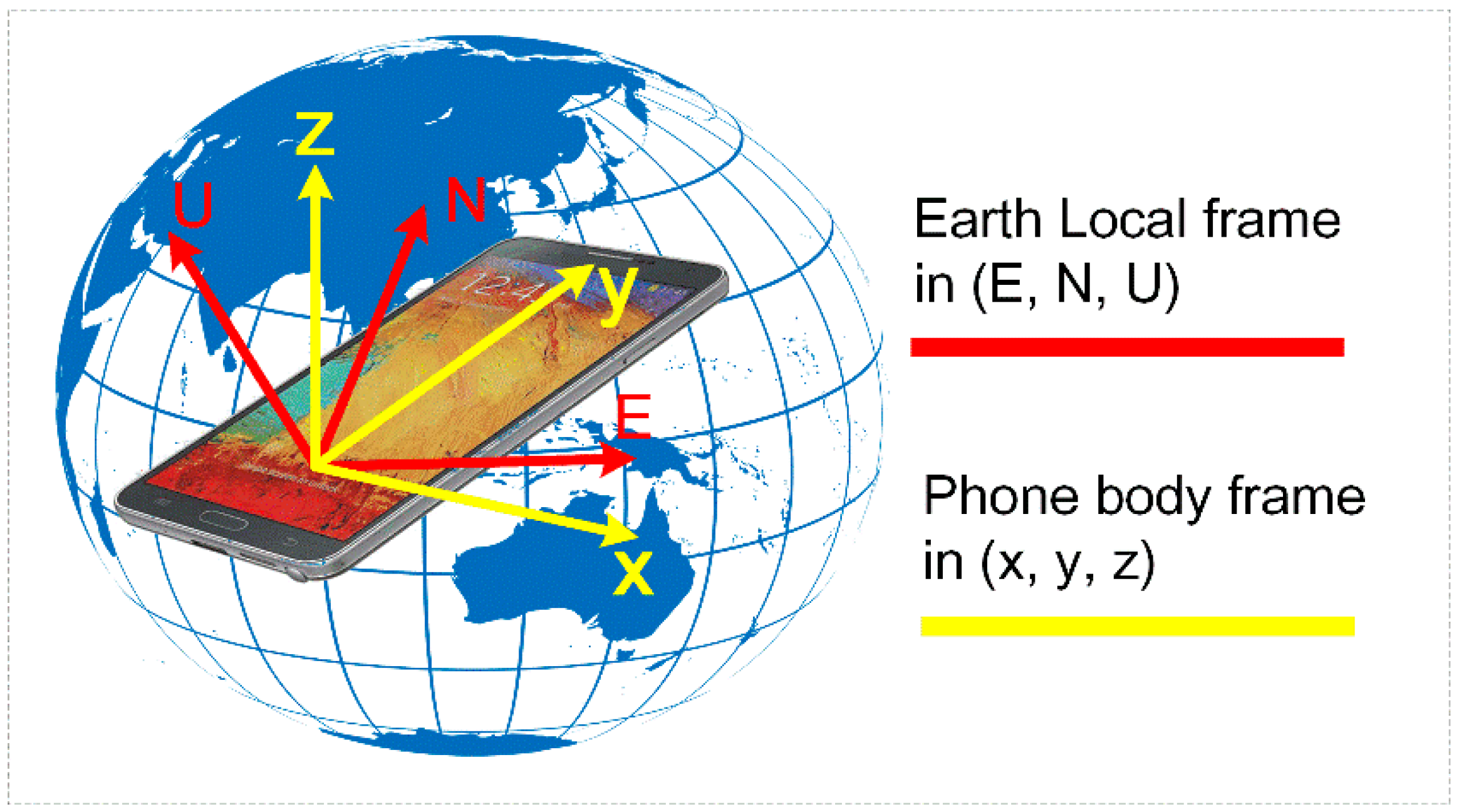
2.2. MEMS Built-in Smartphone

Since inertial navigation technology is capable of working in all environment where GNSS has difficulties, MEMS inertial technology is regarded as a possible complement to GNSS. With the strong growth of MEMS technology, multiple MEMS sensors are built into smartphones, typically including a three-axis accelerometer, three-axis gyroscope, and three-axis magnetometer, which are basic parts in a pedestrian navigation system. As shown in Figure 2, we determine the smartphone attitude when the axis orientation of the smartphone body frame is specified with respect to the Earth frame. The phone’s x-axis is horizontal and points to the right, while the z-axis is perpendicular to the x-y plane and completes a right-handed coordinate system.

We can obtain the sensor observations with the android.hardware.SensorEvenListener API, where the observed values are provided in the order of x-, y-, and z-axes in the body frame. Thus, it is important to obtain a clear axial distribution of the phone’s sensor. For pedestrian navigation, PDR is a conventional method to make use of the sensor observations, which exploits the kinematics of human walking. The measurements of accelerometers are utilized for step detection and step length estimation. Heading can be obtained through nine-axis attitude determination, which is typically called the AHRS (attitude and heading reference system). Most of the AHRS algorithms use the gyroscope to compute the continuous relative attitude, and use the accelerometer and magnetometer for absolute updates and sensor bias correction.

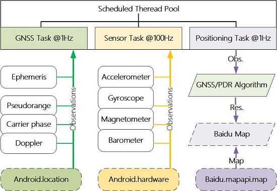
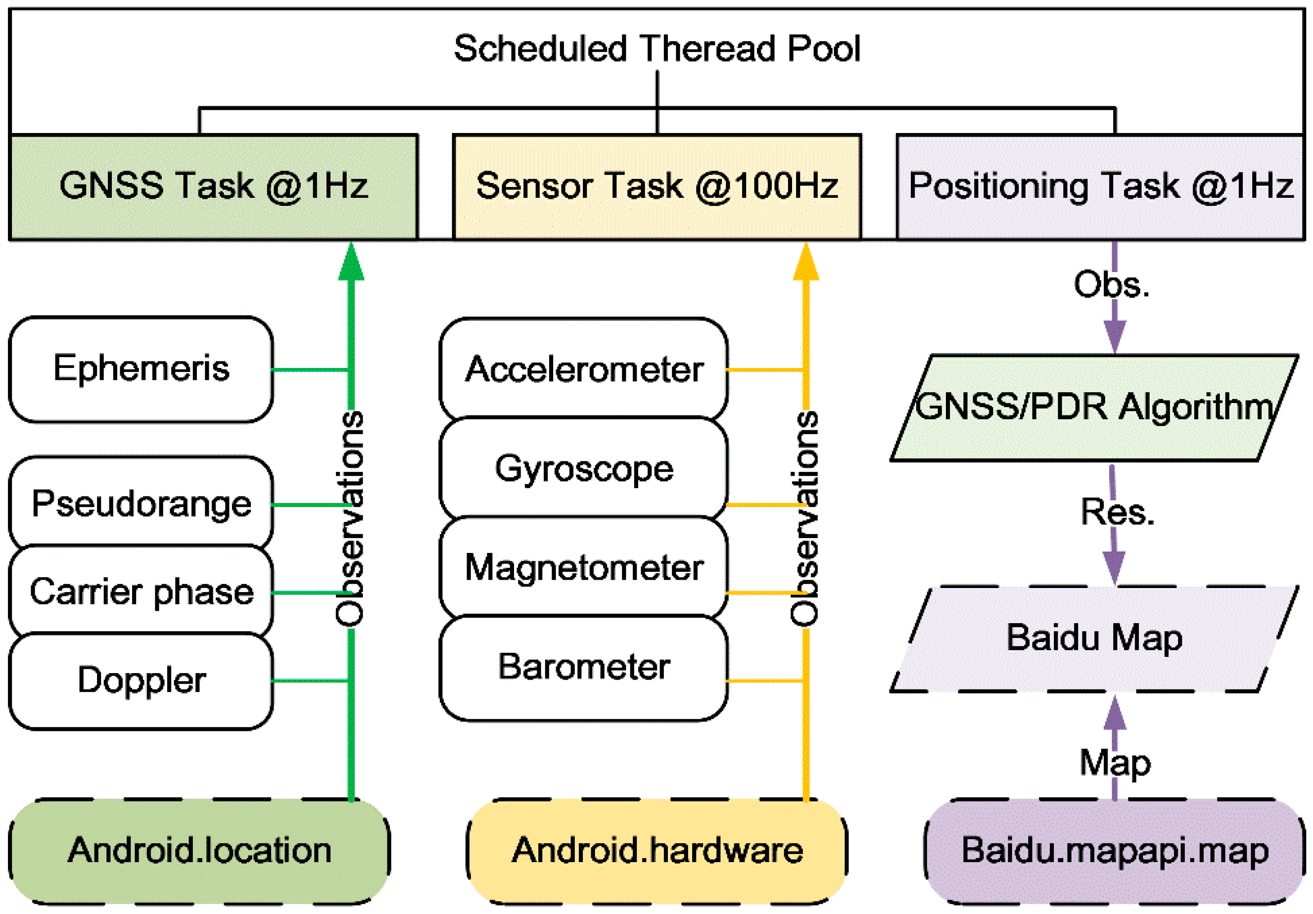
2.3. Design of Walker Application

The advantage of a smartphone could be fully exploited if the observation acquisition and computation as well as the result presentation can be integrated into on one single application. Based on this consideration, we designed this application, called Walker, for pedestrian navigation using mass-market devices in an urban environment. The key components of Walker and the data flow are given in Figure 3. First, the GNSS observations and ephemeris are obtained from the location API. The MEMS observations are obtained from the hardware API. Then these data are processed by a GNSS/PDR algorithm, whose specific method will be discussed in the next section. Finally, the computed navigation solution is displayed on the smartphone map, which is supported by Baidu.mapapi.

There are two essential parts in the application design that should be emphasized—one is the GNSS observation capture and the other is the GNSS and MEMS data synchronization. Since the GNSS raw measurements and ephemeris are supported in the new location API, these observations should be generated accurately. As mentioned in Section 2.1, the pseudorange generation of different navigation satellite systems should take into account the difference in system times. For GNSS data, a GNSS task is created in the application to obtain observations at 1 Hz, while a MEMS task is used to obtain sensors data at 100 Hz. Supported by Location API of Android, GNSS has a maximum data output rate of 1 Hz, which is enough to meet the navigation needs of normal users. Then, a positioning task is run at 1 Hz to read and process these two types of data simultaneously. All tasks are registered in the scheduled thread pool so that the source sensor data can be managed in an orderly manner.

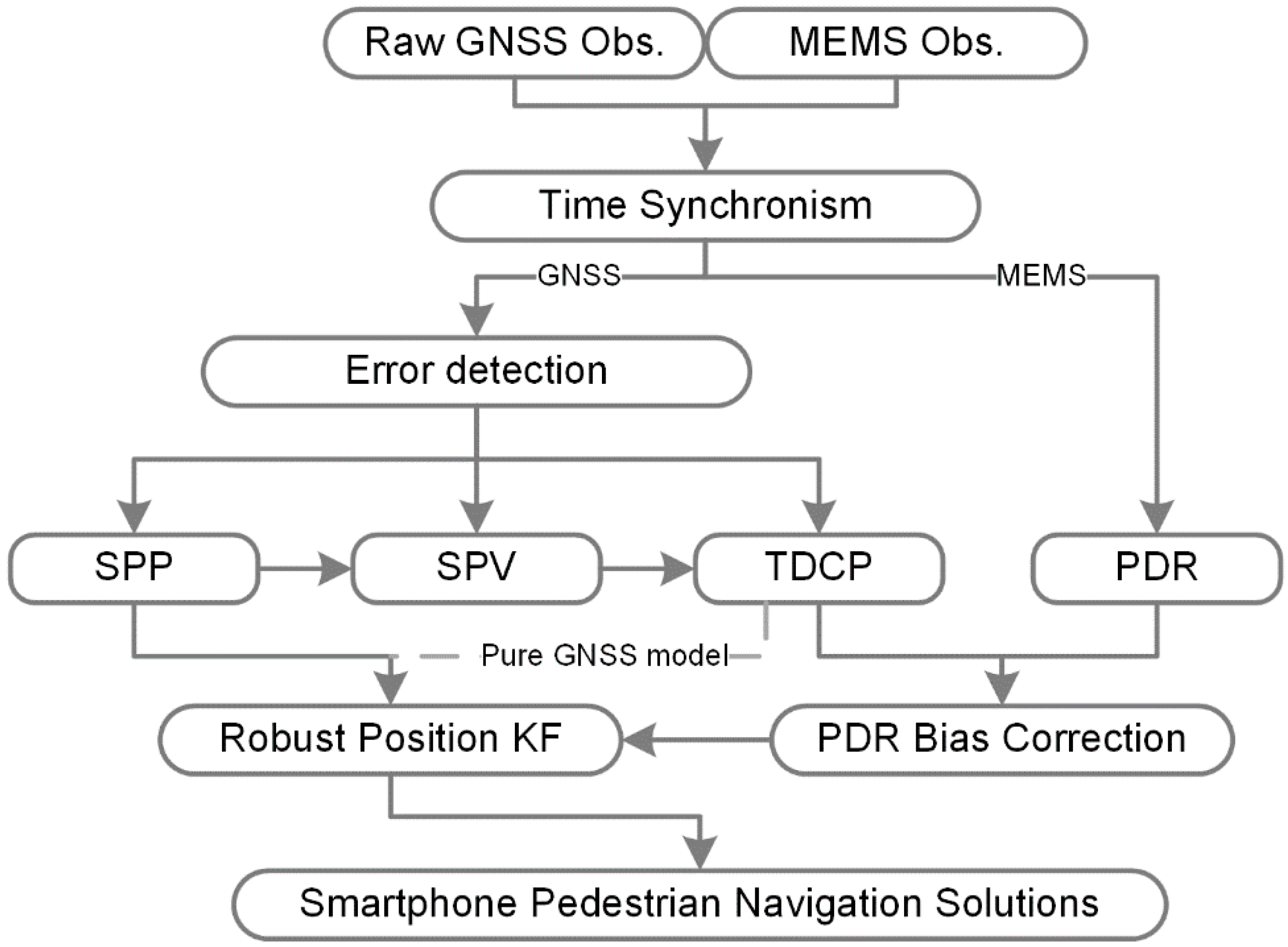
3. Fusion Method of GNSS and MEMS in Smartphones

Capitalizing on the complementary characteristics of GNSS and PDR systems, a more accurate and robust navigation solution is provided through their combination than either could achieve alone. The fusion strategy of these two systems is shown in Figure 4.

Firstly, the observations of GNSS and the MEMS are obtained and synchronized from the android API. Then, for the GNSS process module, the gross errors are detected according to the SNR and pseudorange rate, and the position and velocity are estimated by single-point positioning (SPP) and a single-point velocity (SPV) determination algorithm. Furthermore, the precise velocity estimation is realized by the time-differenced carrier phase (TDCP) technique. Meanwhile, the three-dimensional (3-D) relative position changes are computed through the PDR system with the IMU, magnetometer, and barometer observations. Thereafter, the bias of step length and heading of the modeled PDR system is corrected through a sliding window. Finally, a robust Kalman filter is applied to fuse the position change and GNSS positioning. If the pure GNSS processing model is chosen, the position change is fed by the TDCP instead of 3-D PDR. Some key techniques to implement the fusion of GNSS and PDR are discussed in this section.

3.1. GNSS Position and Velocity Estimation

Multi GNSS constellations can improve positioning accuracy, especially in harsh conditions, even when the number of satellites available in one constellation is less than four. Since there exists inter-system bias (ISB) between different constellations, the range measurement will contain an additional error that degrades the GNSS positioning accuracy [17,18]. The ISB estimated using mass market receivers are noisier than obtained using geodetic receivers [19]. Generally, the ISBs are parameterized and estimated in the positioning equation. Choosing GPS as a reference system, the ISB of BDS (BeiDou System) to GPS should be extended into the GNSS positioning equation [20]:

$$\underset{Z}{\underbrace{\left[\begin{array}{c}{R}_G^1-{\rho }_0^1\\ ⋮\\ R_G^k-{\rho }_0^k\\ R_B^{k+1}-{\rho }_0^{k+1}\\ ⋮\\ R_B^n-{\rho }_0^n\end{array}\right]}}=\left[\begin{array}{ccccc}\frac{x_0-x_G^1}{{\rho }_0^1}& \frac{y_0-y_G^1}{{\rho }_0^1}& \frac{z_0-z_G^1}{{\rho }_0^1}& 1& 0\\ ⋮& ⋮& ⋮& ⋮& ⋮\\ \frac{x_0-x_G^k}{{\rho }_0^k}& \frac{y_0-y_G^k}{{\rho }_0^k}& \frac{z_0-z_G^k}{{\rho }_0^k}& 1& 0\\ \frac{x_0-x_B^{k+1}}{{\rho }_0^{k+1}}& \frac{y_0-y_B^{k+1}}{{\rho }_0^{k+1}}& \frac{z_0-z_B^{k+1}}{{\rho }_0^{k+1}}& 1& 1\\ ⋮& ⋮& ⋮& ⋮& ⋮\\ \frac{x_0-x_B^n}{{\rho }_0^n}& \frac{y_0-y_B^n}{{\rho }_0^n}& \frac{z_0-z_B^n}{{\rho }_0^n}& 1& 1\end{array}\right]·\left[\begin{array}{c}\delta x\\ \delta y\\ \delta z\\ c·\delta t_G\\ c·\delta t_{G-B}\end{array}\right]$$

(2)

where the subscripts G and B represent GPS and BDS, while the superscript k is the k-th GNSS satellite. $\left(x_0,y_0,z_0\right)$ is the approximate receiver position and $\left(x^k,y^k,z^k\right)$ is the satellite coordinate computed by ephemeris. R is the pseudorange measurement computed from Equation (1). ${\rho }_0^k$ is the distance between the approximate receiver position and satellite, plus corrected atmospheric errors, plus corrected relativistic effects. $\left(dx, dy,dz\right)$ is the correction to the approximate receiver position, and $d{t}_G$ is receiver clock error of the GPS satellite. Meanwhile, the ISB of BDS to GPS is also estimated in Equation (2). Similarly, the ISBs of GLONASS and GALILEO can also be parameterized and added in this equation, at which point the design matrix H should also be extended. If the number of available satellites is not less than the number of unknows, the receiver position can be obtained after a few iterations.

It is crucial for many dynamic applications to measure the velocity precisely. A greater accuracy of velocity estimation can be obtained by processing differences of consecutive carrier phase measurements, compared with Doppler-based velocity and differencing consecutive positions from SPP. The time difference between the carrier phase observations $\varphi$ at two successive epochs, $t_j$ and $t_{j-1}$, can be expressed as [21]:

$$\begin{array}{cc}\hfill \lambda ·\Delta \varphi & =\lambda ·\left({\varphi }_{t_j}-{\varphi }_{t_{j-1}}\right)\hfill \\ & =\Delta \rho +c·\Delta d{t}_u+c·\Delta d{t}_s+\Delta d_{eph}-\Delta d_{iono}+\Delta d_{trop}+\Delta \eta \hfill \end{array}$$

(3)

where $\Delta$ is the differencing operator, $\Delta d{t}_u$ and $\Delta d{t}_s$ are the differenced user receiver and satellite clock error, respectively, $\Delta d_{eph}$, $\Delta d_{iono}$, and $\Delta d_{trop}$ are the differenced residuals of ephemeris, ionosphere, and troposphere errors, and $\Delta \eta$ indicates the differenced multipath and receiver noise. $\Delta \rho$ is the change in the geometric range between two epochs. $\Delta d{t}_s$, $\Delta d_{iono}$, and $\Delta d_{trop}$ are negligible between epochs, and $\Delta d_{eph}$ is negligible too if the ephemeris errors remain quasi-constant between epochs. Thus, Equation (3) can be simplified and linearized as

$$\lambda ·\Delta \varphi -\Delta D+\Delta g=-e_{t_j}·\Delta r_u+c·\Delta d{t}_u+\Delta \epsilon$$

(4)

with

$$\begin{array}{l}\Delta g=e_{t_j}·r_{u,t_{j-1}}-e_{t_{j-1}}·r_{u,t_{j-1}}\\ \Delta D=e_{t_j}·r_{s,t_j}-e_{t_{j-1}}·r_{s,t_{j-1}}\end{array}$$

(5)

where $r_u$ and $r_s$ are the receiver position and satellite position, respectively, while $e$ is the receiver-satellite unit vector. The user position change $\Delta r_u$ and receiver clock change $\Delta d{t}_u$ can be estimated using the weighted least squares method. Assuming $m(m>4)$ in Equation (4), a SNR-based variance covariance matrix can be constructed as follows:

$$\begin{array}{l}\mathsf{\Sigma }=\mathrm{diag}\left(s_1,s_2,\dots ,s_m\right)\\ s_i=a+b·{10}^{\frac{-SN{R}_i}{10}} , i=1,2,\dots ,m\end{array}$$

(6)

in which the constants a and b need to be determined for each type of equipment. Here, the following values have been used: a = 10 m² and b = 150² m² Hz [22].

The user velocity $V_u$ can be derived from the user position change $\Delta r_u$ as follows:

$$V_u=\Delta r_u/\left(t_j-t_{j-1}\right)$$

(7)

and the horizontal position change $\Delta S_{gnss}$ and the heading ${\alpha }_{gnss}$ of GNSS can be expressed as

$$\begin{array}{l}\Delta S_{gnss}=\Vert \left(V_u^E,V_u^N\right)\Vert ·\left(t_j-t_{j-1}\right)\\ {\alpha }_{gnss}=atan2\left(V_u^E,V_u^N\right)\end{array}$$

(8)

where the user velocity $V_u$ is expressed in the local navigation frame, which consists of east (E), north (N), and up (U) components.

3.2. Fusion Filter Design with Improved 3-D PDR

As shown in Figure 4, the error detection of GNSS observations is carried out first. The SNR and pseudorange rate of observations are tested. If the SNR of the smartphone GNSS observation is lower than 15 dB-Hz, the corresponding satellite will be eliminated. If the difference between the pseudorange rate and Doppler is greater than the threshold value (3 m/s is set in our algorithm), this satellite will also be eliminated in this epoch. After error detection, if the number of available satellites is greater than the number of unknowns in the least square equations, the GNSS position and velocity estimations are performed. According to Equation (8), the horizontal position change and the heading of GNSS can be obtained. Thus, the bias of PDR is described as

$$\{\begin{array}{l}\delta S=\Delta S_{gnss}-\Delta S_{pdr}\\ \delta \alpha ={\alpha }_{gnss}-{\alpha }_{pdr}\end{array}$$

(9)

where $\delta S$ and $\delta \alpha$ are the step length bias and the heading bias of PDR, while $\Delta S_{pdr}$ and ${\alpha }_{pdr}$ are the horizontal position change and the heading of PDR, respectively. The PDR system is a relative position system and errors accumulate over time. Since the velocity of the TDCP in Equation (7) is very accurate, the bias correction in Equation (9) will improve the accuracy of PDR. The inaccuracy of heading using GNSS should considered, when the estimated velocity is lower than 5 km/h. Thus, the inaccurate heading of GNSS will not be used to correct PDR heading. The improved PDR can calculate more accurate relative positioning during GNSS signal outage, which is crucial for continuous pedestrian navigation in harsh situations.

In order to continuously provide 3-D relative positioning, the barometer is used to compute any change of altitude. In the aerospace industry and GPS/barometer-augmented navigation systems, a well-known empirical formula is used to covert barometric pressure p to altitude h [23,24]:

$$h=\left(\frac{R·T}{g·M}\right)·\ln \frac{p_0}{p}$$

(10)

where h is the difference between the starting height and the measurement height, R is the universal gas constant (0.31447 J/(mol·k)), g is the gravitational constant at the Earth’s surface (9.80665 m/s² at sea level), M is the molar mass of air (0.0289644 kg/mol), $p_0$ and T are the pressure and temperature at the starting height, and $p$ is the pressure at the measurement height. The commonly used barometer sensors, such as BMP180/182 and LPS331AP, have a low absolute accuracy ranging from −20 to 20 m, but with a high relative accuracy varying within ±2 m. As an accurate estimation of absolute barometric altitude requires calibration, we used the relative altitude that directly determines the user vertical position change.

In our integration method, a robust Kalman filter is employed. The state vector $X_{t_j}$ is composed of three-dimensional position $\left(x,y,z\right)$ expressed in earth-centered earth-fixed frame (e frame) and receiver clock $dt$ error for each system (take GPS as an example), as follows:

$$X_{t_j}={\left[x,y,z,dt\right]}^T$$

(11)

with the subscript $t_j$ indicating the epoch. The system model in the discrete form is given by

$$X_{t_j}={\mathsf{\Phi }}_{t_j,t_{j-1}}·X_{t_{j-1}}+B_{t_{j-1}}·u_{t_{j-1}}+W_{t_{j-1}}$$

(12)

where ${\mathsf{\Phi }}_{t_j,t_{j-1}}$ is the transition matrix from the time $t_{j-1}$ to $t_j$, $u_{t_{j-1}}$ is the system input vector, $B_{t_{j-1}}$ is the input matrix, $W_{t_{j-1}}$ is state noise vector with a distribution $W_{t_{j-1}}:N\left(0,Q_{t_{j-1}}\right)$, $Q_{t_{j-1}}$ is the covariance matrix of state vector. The transition matrix is a unit matrix

$${\mathsf{\Phi }}_{t_j,t_{j-1}}=\underset{4\times 4}{\underbrace{\left[\begin{array}{cccc}1& 0& 0& 0\\ 0& 1& 0& 0\\ 0& 0& 1& 0\\ 0& 0& 0& 1\end{array}\right]}}$$

(13)

The input vector is composed of relative position $\Delta r_u^n=\left(dE,dN,dU\right)$ of two epochs expressed in local navigation frame (n frame) and time-differenced receiver clock error $\Delta dt$, as

$$u_{t_{j-1}}={\left[\Delta r_u^n, \Delta dt\right]}^T$$

(14)

The input matrix is given by

$$B_{t_{j-1}}=\underset{4\times 4}{\underbrace{\left[\begin{array}{cc}{R}_n^e& 0\\ 0& 1\end{array}\right]}}$$

(15)

where $R_n^e$ is the coordinate transformation matrix from n frame to e frame. The covariance matrix of state vector is composed the variance of relative position ${\sigma }_{\Delta r_u^n}^2$ and the variance of time-differenced receiver clock error ${\sigma }_{\Delta dt}^2$ as

$$Q_{t_{j-1}}=\underset{4\times 4}{\underbrace{\left[\begin{array}{cc}{R}_n^e·{\sigma }_{\Delta r_u^n}^2·R_n^e{}^T& 0\\ 0& {\sigma }_{\Delta dt}^2\end{array}\right]}}$$

(16)

Here, if the number of available satellites is more than four, the relative position $\Delta r_u^n$ can be estimated from TDCP, and the time differenced receiver clock error $\Delta dt$ can also be computed. The estimation accuracy of $\Delta r_u^n$ determines the value of ${\sigma }_{\Delta r_u^n}^2$, which is generally between ${0.02}^2{\mathrm{m}}^2$ and ${0.2}^2{\mathrm{m}}^2$. The variance of time-differenced receiver clock error ${\sigma }_{\Delta dt}^2$ is about $5^2{\mathrm{m}}^2$. If the number of available satellites is less than four, the TDCP will not work. Thus, the relative position $\Delta r_u^n$ of PDR will be take into consideration with an accuracy of approximately ${0.1}^2 {\mathrm{m}}^2$. The time differenced receiver clock error will be set to zero with an accuracy of ${100}^2 {\mathrm{m}}^2$, that means the receiver clock error will be re-estimated in the measurement update.

The measurement model is given by

$$Z_{t_j}=H_{t_j}·\delta X_{t_j}+R_{t_j}$$

(17)

where the construction of measurement residual vector $Z_{t_j}$ and design matrix $H_{t_j}$ are shown in Equation (2), $R_{t_j}$ is measurement noise vector with a distribution $R_{t_j}:N\left(0,{\mathsf{\Sigma }}_{t_j}\right)$, ${\mathsf{\Sigma }}_{t_j}$ is obtained from SNR-based weighting scheme shown in Equation (6), $\delta X_{t_j}$ is the correction to the initial position of linearization. The predicted position from Equation (12) is used as initial position of linearization, and the user position $X_{t_j}$ can be obtained through a few iterations in Equation (17).

It can be found that the Kalman filter is used to fuse the relative position and the absolute position of SPP. Since the relative position is accurate and the process noise is small, the noisy position of SPP will be smoothed through the weighted action of the Kalman filter. In addition, the fault of the measurement update should be detected and eliminated. Thus, the posteriori residuals of the Kalman filter are tested. If the posteriori variance ${\sigma }^2$ exceeds the threshold ($6^2{\mathrm{m}}^2$ is set in our algorithm), the satellite with max posteriori residuals would be excluded and the epoch would be reprocessed. The posteriori variance is ${\sigma }^2=(V^{T}PV/n)$. Here, n is the number of used satellites, V is the posteriori residuals vector of the Kalman filter, and P is the weight matrix of the observations vector. As described at the beginning of this section, the SNR and pseudorange rate of observations are first tested to detect the error of GNSS observations. We call this a prior gross error detection. Finally, the posteriori error detection is used for Kalman filter. In this way, the gross error of GNSS observations can be detected and eliminated step by step, that improve the reliability of positioning results.

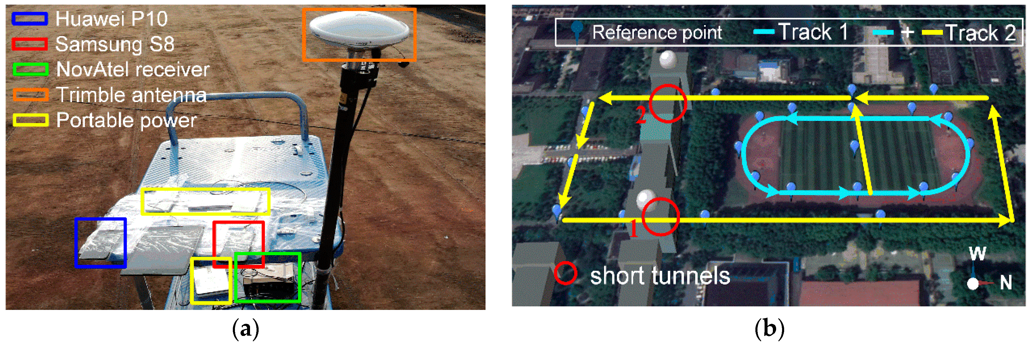
4. Field Test Results and Discussions

In this section, the Walker application is tested in the field in terms of characteristics of observation, accuracy of static GNSS positioning, and kinematic navigation performance. The GNSS observations are assessed in terms of C/N0, station single-difference pseudorange residuals, pseudorange rate, phase rate, and Doppler. The stochastic errors of the MEMS sensors are analyzed using the Allan variance method. The static GNSS data were collected under a normal open sky with devices, as shown in Figure 5, including Samsung S8 and Huawei P10 smartphones as well as a geodetic-quality antenna (Trimble Zephyr-2) and a receiver (NovAtel ProPak6). The kinematic track shown in Figure 5 is in a playground surrounding the field under open sky, except for several parts shielded by nearby trees and buildings. There are some reference points along the track whose coordinates are determined by professional RTK equipment previously. The accuracy of RTK fixed solution is centimeter level, which ensures the accuracy of reference point. Two reference points in short tunnels are measured by total station. In addition, the accuracy comparison of all results is in WGS84 coordinate system.

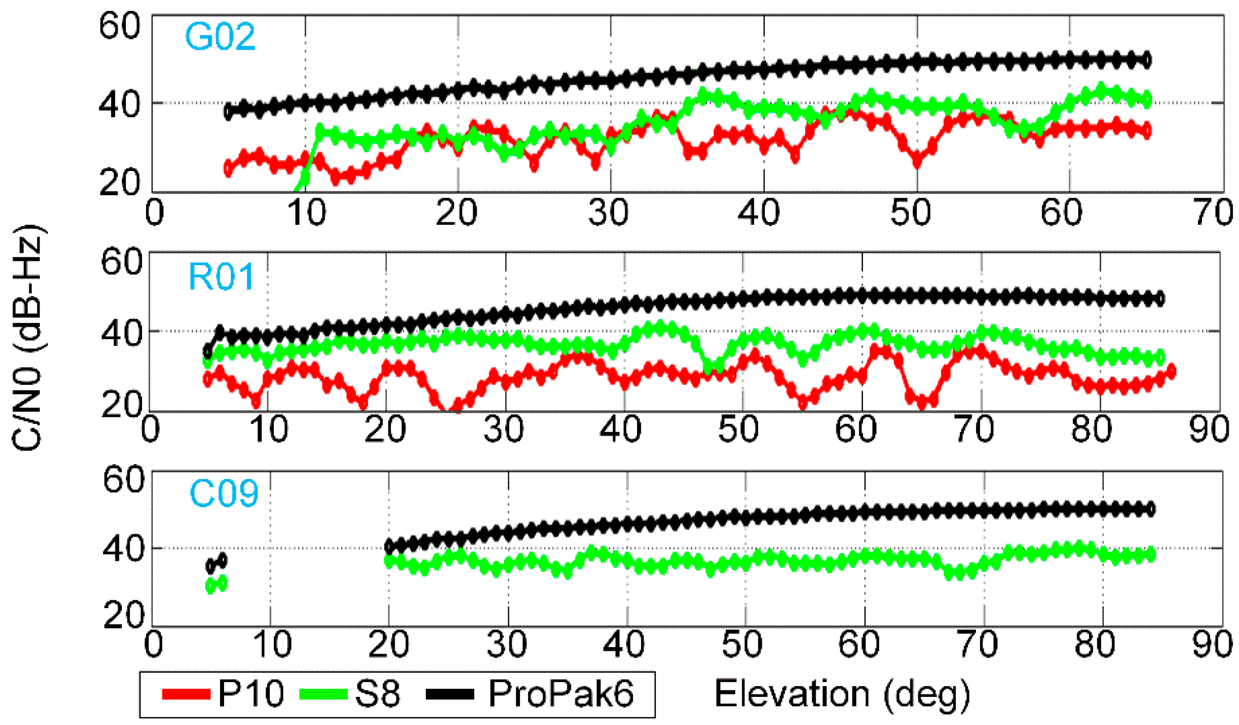
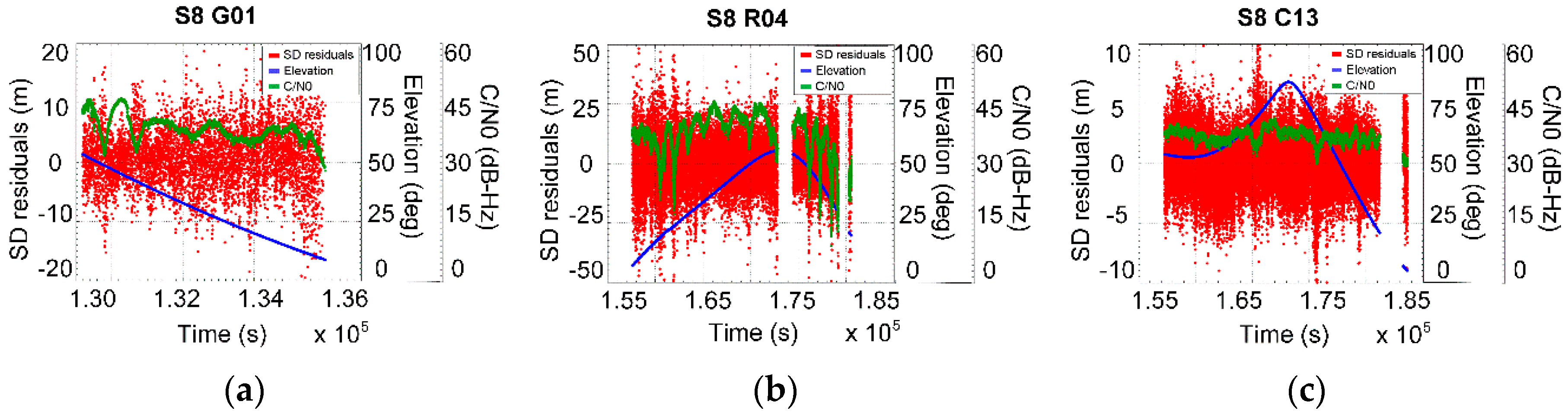
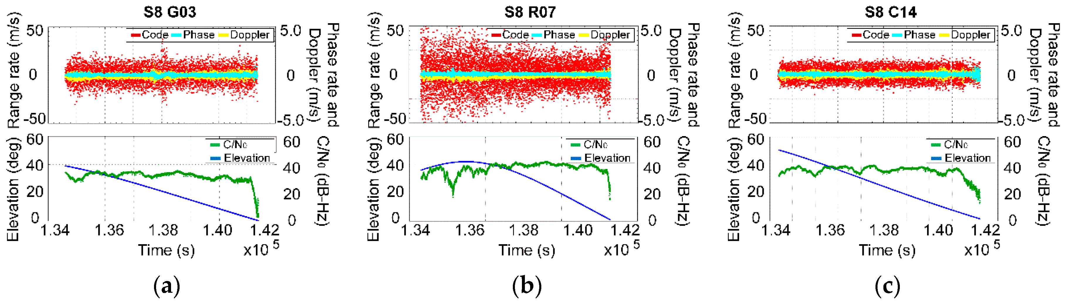
4.1. Characteristics of Smartphone GNSS Observations

The C/N0 obtained from a GNSS receiver is the result of the gains and losses along the complete transmission chain, providing critical performance data for characterizing a variety of accessible signals. The average C/N0 of S8, P10, and the geodetic devices are analyzed with respect to the elevation angle. As illustrated in Figure 6, the C/N0 values measured with two smartphones are approximately 10 dB-Hz lower than the values obtained from a geodetic-quality device, which indicates the quality of the smartphone observations. For smartphones, the C/N0 values vary more significantly, while they are more stable in geodetic devices. the C/N0 values of the employed Samsung and Huawei smartphones also show differences, with the S8 being slightly larger than the P10 as well as more stable.

For the smartphone devices with a built-in GNSS antenna, it is hard to carry out the zero-baseline experiment without external hardware. Thus, we used a short-baseline experiment to determine the pseudorange noise of smartphones with the geodetic devices as a reference. The single-difference combination between a smartphone and a nearby (less than 1 m) geodetic receiver is defined as

$$\Delta P_{rb}^j=\Delta {\rho }_{rb}^j+c·\Delta d{t}_{rp}+\Delta M_{rb}^j+\Delta {\epsilon }_P$$

(18)

where $\Delta$ is the differencing operator, the subscripts r and b represent smartphone receiver and geodetic receiver, while the superscript j is the j-th GNSS satellite. $P$ is the pseudorange observation, $\rho$ is the ranges between the satellite and the station calculated using broadcast ephemeris and prior station coordinates, c is the speed of light, dt is the receiver-closk error, M is multipath error, $\epsilon$ is the pseudorange noise. As the satellite and atmospheric delay errors were differenced and the receiver-clock bias estimated with a known receiver position, the SD residual ($\Delta M_{rb}^j+\Delta {\epsilon }_P$) mainly represents the noise of the pseudorange observations plus multipath error. Assuming that the smartphone pseudorange noise is much larger than that of a geodetic-level device, the SD residual is basically affected by the smartphone pseudorange noise and multipath error. Figure 7 shows the comparison of station single-difference (SD) pseudorange residuals. The smartphones’ SD residuals range from −20 to 20 m for GPS and GLONASS pseudorange, while the geodetic device’s SD residuals range from −1 to 1 m. Thus, the smartphones’ pseudorange measurements have a much higher noise level than that of a geodetic-quality device. However, the SD residuals of BDS pseudorange obtained from S8 vary within ±10 m, which is much smaller compared with GPS and GLONASS. The statistic of SD pseudorange residuals of GPS, GLONASS, and BDS for the S8 smartphone are 15.93 m, 29.87 m, and 5.17 m, respectively, reflecting the characteristics of the code noise of smartphone GNSS.

As illustrated in Figure 8, the C/N0 values showed a strong relationship with the smartphone SD residuals, and gross errors were present when the C/N0 decreased to 20 dB-Hz. As expected, for the geodetic receiver, the SNR is smaller when the satellite is tracked at lower elevation angles, which justifies the elevation-dependent weighting. However, for the smartphones, such a correlation is not as clear because the SNR varies more significantly, regardless of the elevation angle. Therefore, SNR-dependent weighting is more appropriate during smartphone GNSS data processing.

Figure 9 shows the comparison of the pseudorange rate, phase rate, and Doppler data. The majority of GPS and GLONASS pseudorange rates vary within ± 10 m/s, while phase rates and Doppler vary within ± 0.2 m/s. Similar to the case of the GNSS SD residuals, the pseudorange rate of BDS has a higher accuracy than that of GPS and GLONASS, but the accuracy of Doppler and phase rates for smartphone GNSS are comparable. The meter-level pseudorange rate noise is approximately two orders of magnitude larger than the phase rate and the Doppler. Therefore, the phase and Doppler observations show a centimeter per second precision and can be used to derive user velocity and detect observation error.

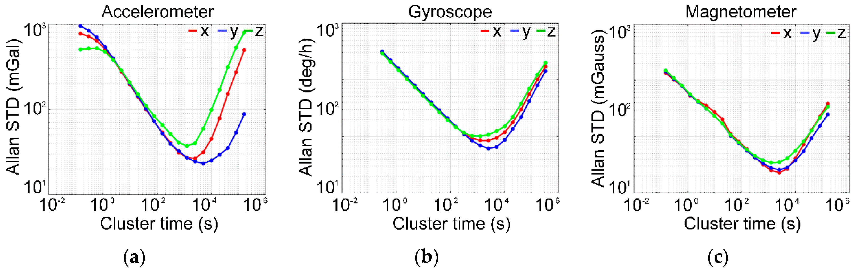
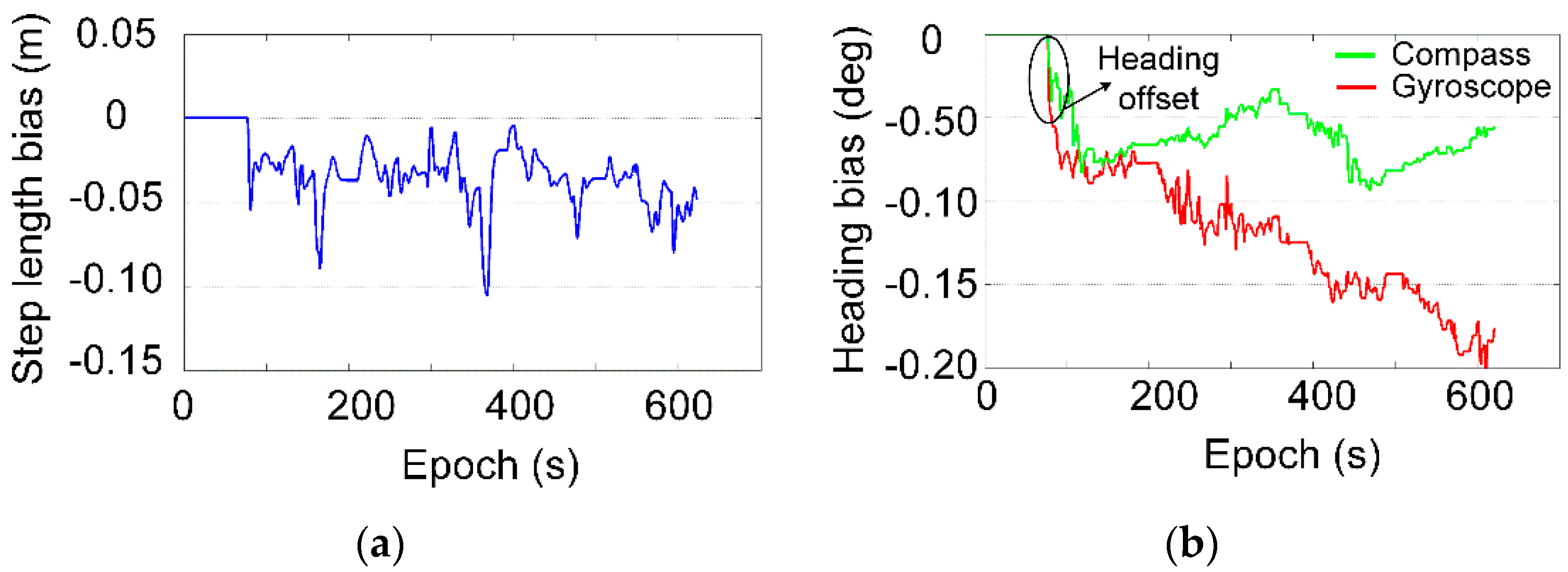
4.2. Stochastic Error of Smartphone MEMS Sensors

The outputs of MEMS sensors fixed inside a smartphone are not perfect and suffer from some error sources, including bias, scale factor, axis misalignment, and non-orthogonality, as well as impact of temperature. The Allan variance is a method that can analyze the sensors’ frequency stability in the time domain and determine the characteristics of the underlying random process. As shown in Figure 10, the log-log plot of the Allan standard deviation versus the cluster time is obtained from about 10.48 hours static data obtained from a Huawei P10 smartphone. For the three-axis accelerometer, three main noises are identified, including a velocity random walk in the −1/2 slope part, a bias instability in the 0 slope part, and a rate random walk given by the +1/2 slope part. Similar findings were obtained for the three-axis gyroscope and three-axis magnetometer, including an angular random walk in the −1/2 slope part, a bias instability in the 0 slope part, and a rate random walk given by the +1/2 slope part. The mean values of accelerometer, gyroscope, and magnetometer bias instability are 28.60 mGal, 7.38 deg/h, and 0.28 mGauss, respectively, and the values on each axis are of same order of magnitude.

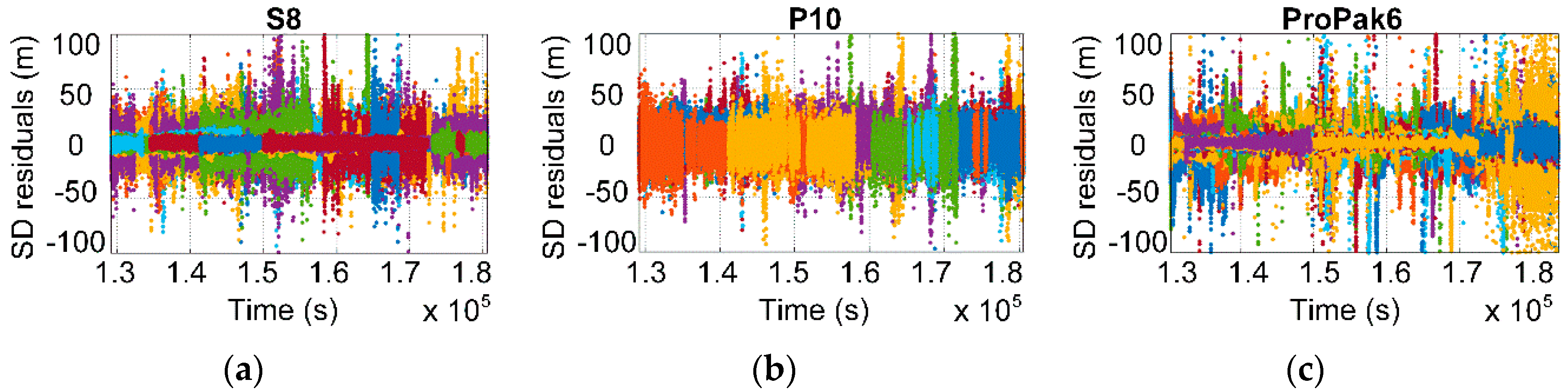
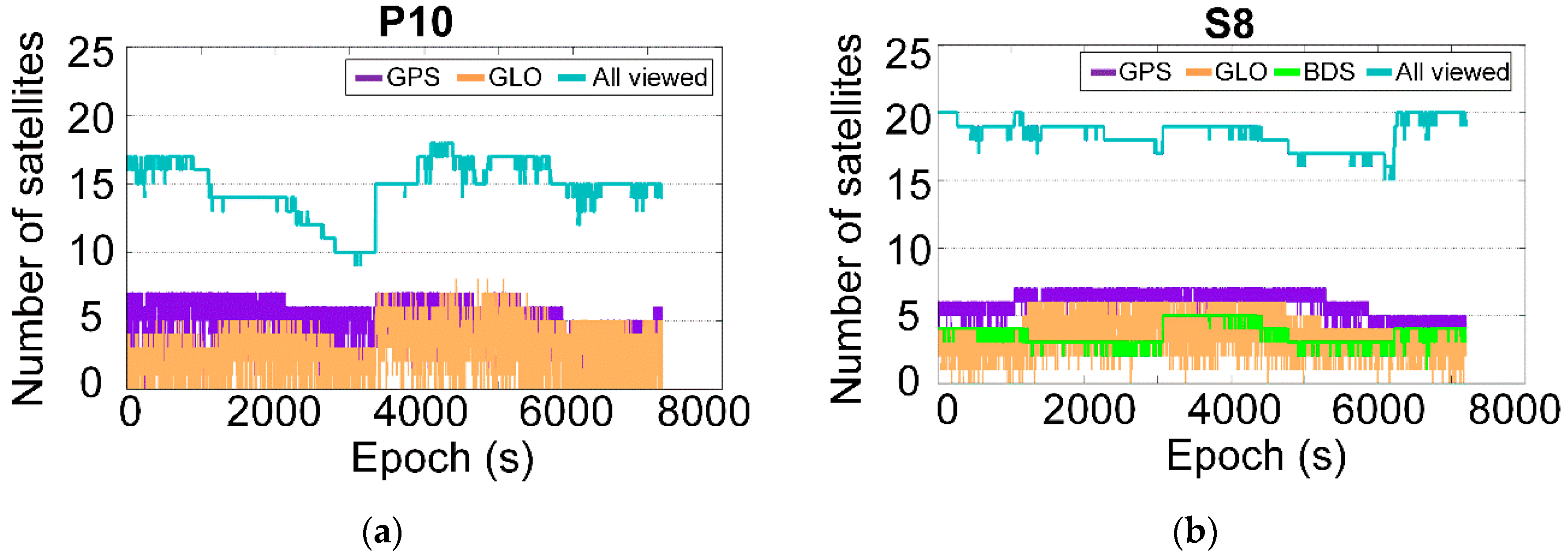
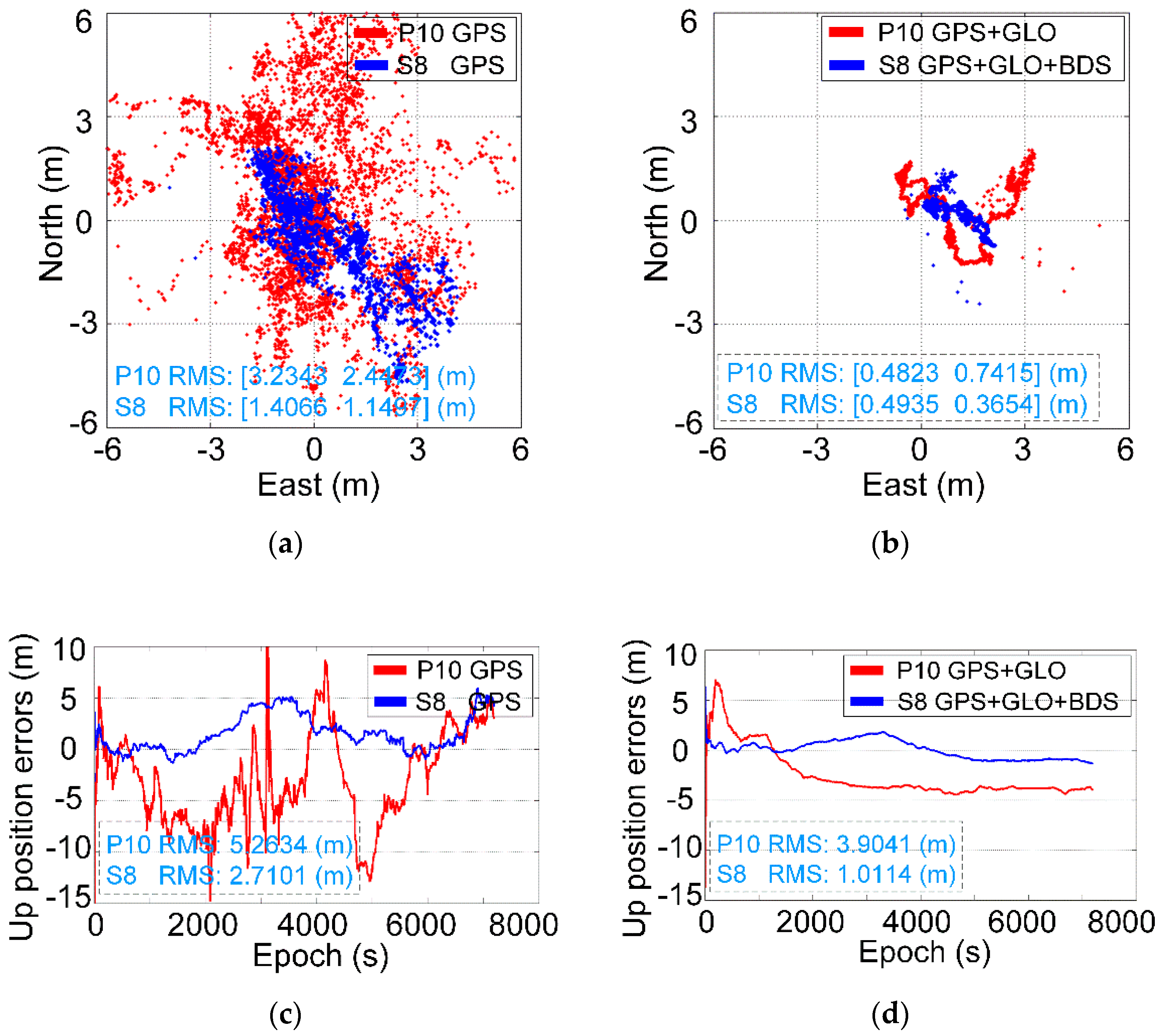
4.3. GNSS Static Positioning Analysis

In this experiment, the GNSS observations of P10 and S8 smartphones are processed with the proposed algorithm as shown in Figure 4, where the pure GNSS model is selected. Figure 11 shows the number of GPS, GLONASS, and BDS satellites viewed. For the S8 smartphone, there are about 19 visible GNSS satellites, while it declines to 15 for the P10, due to the absence of BDS. After error detection, only five to seven GPS satellites were found to be used in the positioning process, and there were about two to four GLONASS satellites and three BDS satellites added for the GNSS positioning process.

As illustrated in Figure 12, the GNSS position errors in the east, north, and up directions decrease dramatically compared to the error level when only GPS is used. The horizontal position errors of S8 GPS reach to more than 2 m, and it is even worse for P10. When GNSS observations are applied, the horizontal positioning accuracy of P10 and S8 reached the decimeter-level, and the filtering positions show lower noise. Meanwhile, the root mean square (RMS) error of the up-vertical position is reduced by 2 m, and the up-vertical accuracy of the S8 GNSS is approximately 1 m. The increase of GLONASS and BDS enhances the geometry of the satellites, which decreases the position dilution of precision; thus, the positioning accuracy was improved.

As shown in

Table 1. The statistics of root mean square (RMS) errors of different positioning methods, including GNSS processed by single-point positioning (SPP), and results of the GNSS chipset built-in smartphones and GNSS processed by our proposed method (positioning filtering).

		East (m)	North (m)	Up-Vertical (m)
Huawei P10	SPP	5.3164	7.9280	14.2151
	GNSS chipset	1.5638	1.4062	4.8635
	Position filtering	0.4823	0.7415	3.9041
Samsung S8	SPP	3.8822	4.2733	8.7364
	GNSS chipset	1.6545	3.8972	3.2401
	Position filtering	0.4935	0.3654	1.0114

, the horizontal position RMS error of SPP reaches 5 m, and it reaches about 10 m in the up-vertical direction. It is hard to achieve 1-m-level positioning accuracy with only a noisy smartphone pseudorange. There is some improvement over SPP for smartphone GNSS chipsets, especially in the vertical direction. As such, the traditional phone’s GNSS positioning is labeled as being within a few meters’ accuracy for public users. Benefiting from the release of android raw GNSS measurements, our proposed positioning method exhibits an obvious improvement. Its horizontal position RMS declines to 0.5 m, as well as improving in the vertical component. The proposed method is capable of achieving 1-m-level accuracy because the noisy pseudorange position is smoothed by the accurate time-differenced carrier phase. In addition, it is convenient to be implemented in mass-market smartphones without external corrections or reference stations.

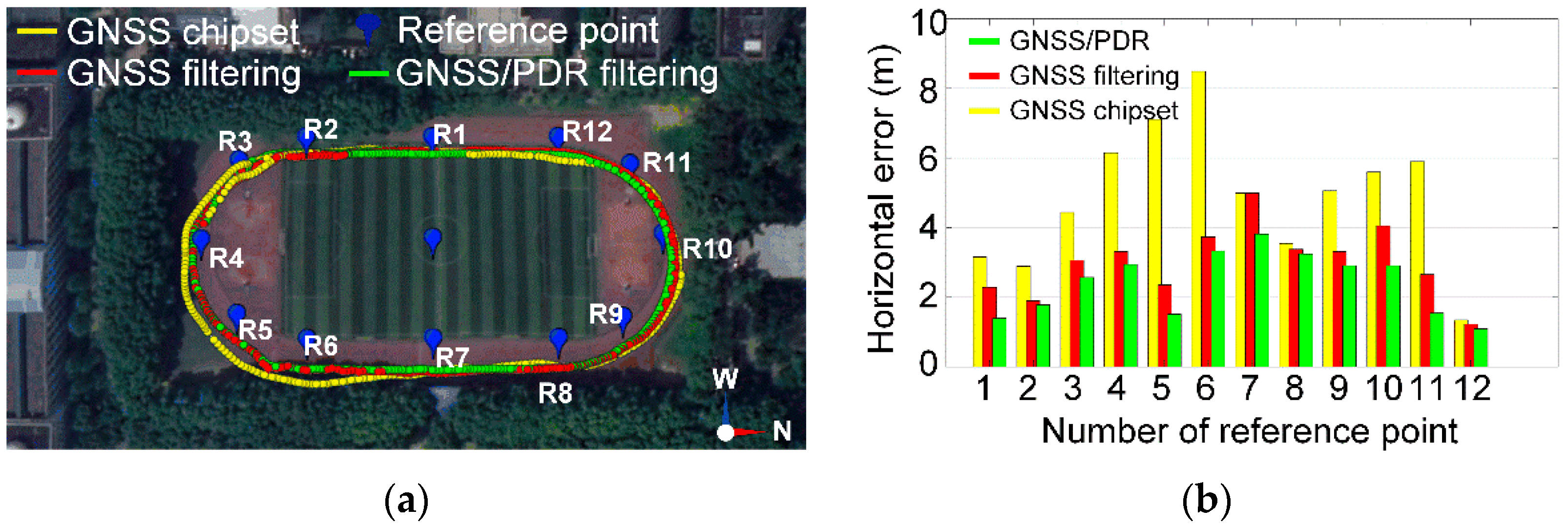
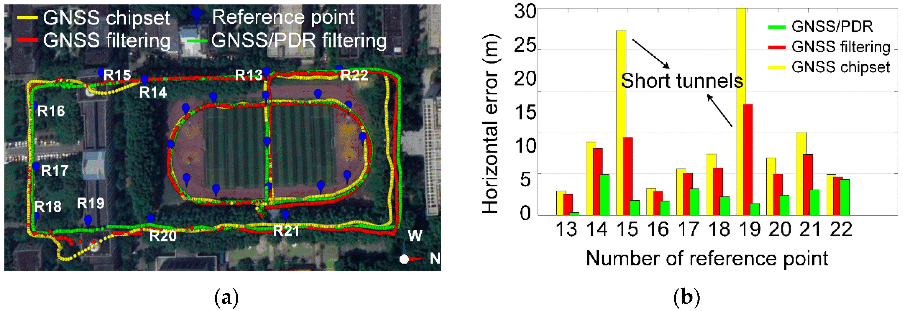
4.4. Integrated Navigation Performance Analysis

In the kinematic experiment, the two tracks shown in Figure 5 are tested. The PDR bias correction with the TDCP is verified in this approximately 500-m track (track 1). The aim of the other experiment, inclusive of track 1 and track 2, is to test the performance of the GNSS/PDR integration algorithm. During the kinematic test, the employed P10 smartphone is a handheld model, and the initial heading is given by the smartphone compass sensor.

Figure 13 presents the track comparison and the horizontal position errors computed from the reference points. It is found that the track of the GNSS chipset does not agree well with the reference, while there is some improvement in the track involving GNSS filtering only. However, it is not smooth and accurate due to the unstable quality of GNSS observations. In particular, in the south of track, the high buildings and trees provide shelter from the line of sight of GNSS signals, in addition to causing a strong multipath effect. The fusion of GNSS and PDR can make up for the discontinuous positioning, due to the accurate recursion ability of the trained PDR. The horizontal position errors of integrated GNSS and PDR are about 1 m to 3 m, while the errors of the GNSS chipset and the GNSS filtering-only approaches are twice as much. The RMS values of the three tracks are 5.28 m, 3.18 m, and 2.57 m, respectively, which indicate the kinematic positioning accuracy of the proposed method in a normal pedestrian environment.

As illustrated in Figure 14, the step length bias and heading bias are estimated in the integrated GNSS and PDR navigation. It can be seen that the estimated step length bias is approximately −0.025 m with few fluctuations. The comparison of the heading bias demonstrates that there is an offset between the initial heading obtained from the smartphone compass and the direction in which the user is moving. The error of the gyroscope heading increases linearly with time, and the error of the compass heading shows periodic variation with time. Generally, the linearly increased error of the gyroscope heading is mainly caused by gyroscope bias, and the periodic variation of the compass heading could be influenced by magnetic disturbances. The precise estimation of the PDR bias indicates that the improved PDR system functions as a continuous relative position estimator, which plays an important role in urban pedestrian navigation.

Figure 15 shows the comparison of kinematic tracks in a poor observation environment. When going through short-distance tunnels, the GNSS filtering-only approach exhibits an outage, and the GNSS chipset also diverges to the wrong position. In this case, where GNSS signals are degraded or not available, sensor fusion has an obvious advantage. The integrated GNSS and PDR approach can provide continuously reliable user positions. The RMS values of three tracks are 12.17 m, 7.12 m, and 2.87 m, respectively. By comparing the GNSS-only results in Figure 12, Figure 13, and Figure 15, the GNSS observations show a large difference in positioning performance, which is mainly affected by the complex multipath and signal quality. With a discontinuous GNSS carrier phase, it is hard to smooth the noisy pseudorange. Moreover, the cycle slip and gross errors increase in degraded-observation conditions. These statistics of position errors indicate that the proposed method can bridge the outages of GNSS, as well as keep a 2-m-level accuracy in harsh observation scenarios.

5. Conclusions

We introduced a dedicated android smartphone application named Walker, which provides continuous and precise pedestrian navigation by fusing GNSS and MEMS sensors. Some key techniques were discussed, including source observations generation and synchronization as well as the integration of GNSS and PDR algorithms.

Then, a series of field tests was carried out to validate the proposed Walker application. The quality assessment of android GNSS observations indicated that the time-differenced carrier phase can smooth noisy pseudorange in the positioning domain. The low-cost sensor output was imperfect; the bias should be calibrated. The static experiment results demonstrate that the proposed method is effective to achieve 1-m-level accuracy without the assistance of external corrections or reference stations. The kinematic experiment showed that this method can bridge the outage of GNSS, in addition to achieving an accuracy within two meters for pedestrian navigation. In summary, the release of android GNSS observations from mass-market smartphones facilitates the achievement of high-precision positioning for mass-market users, and the fusion of smartphone GNSS and PDR enhances pedestrian navigation in urban environments.

References

1. Verhagen, S.; Odijk, D.; Teunissen, P.J.G.; Huisman, L. Performance improvement with low-cost GNSS receivers. In Proceedings of the 2010 5th ESA Satellite Navigation Technologies and European Workshop on GNSS Signals and Signal Processing (NAVITEC), Noordwijk, The Netherlands, 8–10 December 2010; pp. 1–8. [Google Scholar]
2. Pesyna, K.M.J.; Heath, R.W.J.; Humphreys, T.E. Centimeter positioning with a smartphone-quality GNSS antenna. In Proceedings of the ION GNSS 2014, Tampa, FL, USA, 8–12 September 2014; pp. 1568–1577. [Google Scholar]
3. Humphreys, T.E.; Murrian, M.; van Diggelen, F.; Podshivalov, S.; Pesyna, K.M.J. On the feasibility of cm-accurate positioning via a smartphone’s antenna and GNSS chip. In Proceedings of the IEEE/ION PLANS 2016, Savannah, GA, USA, 11–14 April 2016; pp. 232–242. [Google Scholar]
4. Hsu, L.T.; Gu, Y.; Kamijo, S. NLOS correction/exclusion for GNSS measurement using RAIM and city building models. Sensors 2015, 15, 17329–17349. [Google Scholar] [CrossRef] [PubMed]
5. Lee, Y.E.; Tao, A.L.; Jan, S.S. Combined Satellite Selection Algorithm and Road Model for GNSS in Constrained Environments. In Proceedings of the ION GNSS 2016, Portland, OR, USA, 12–16 September 2016; pp. 328–334. [Google Scholar]
6. Harle, R. A survey of indoor inertial positioning systems for pedestrians. IEEE Commun. Surv. Tutor. 2015, 15, 1281–1293. [Google Scholar] [CrossRef]
7. Correa, A.; Barcelo, M.; Morell, A.; Vicario, J.L. A review of pedestrian indoor positioning systems for mass market applications. Sensors 2017, 17, 1927. [Google Scholar] [CrossRef] [PubMed]
8. Pham, V.T.; Nguyen, D.A.; Dang, N.D.; Pham, H.H.; Tran, V.A.; Sandrasegaran, K.; Tran, D.T. Highly Accurate Step Counting at Various Walking States Using Low-Cost Inertial Measurement Unit Support Indoor Positioning System. Sensors 2018, 18, 3186. [Google Scholar] [CrossRef] [PubMed]
9. Kang, J.; Lee, J.; Eom, D. Smartphone-Based Traveled Distance Estimation Using Individual Walking Patterns for Indoor Localization. Sensors 2018, 18, 3149. [Google Scholar] [CrossRef] [PubMed]
10. Lachapelle, G.; Gratton, P.; Horrelt, J.; Lemieux, E.; Broumandan, A. Evaluation of a Low Cost Hand Held Unit with GNSS Raw Data Capability and Comparison with an Android Smartphone. Sensors 2018, 18, 4185. [Google Scholar] [CrossRef] [PubMed]
11. Crosta, P.; Zoccarato, P.; Lucas, R.; De Pasquale, G. Dual Frequency mass-market chips: test results and ways to optimize PVT performance. In Proceedings of the ION GNSS 2018, Miami, FL, USA, 24–28 September 2018; pp. 323–333. [Google Scholar]
12. Laurichesse, D.; Rouch, C.; Marmet, F.X.; Pascaud, M. Smartphone applications for precise point positioning. In Proceedings of the ION GNSS 2017, Portland, OR, USA, 25–29 September 2017; pp. 171–187. [Google Scholar]
13. Realini, E.; Caldera, S.; Pertusini, L.; Sampietro, D. Precise gnss positioning using smart devices. Sensors 2017, 17, 2434. [Google Scholar] [CrossRef] [PubMed]
14. Riley, S.; Lentz, W.; Clare, A. On the path to precision—Observations with android GNSS observables. In Proceedings of the ION GNSS 2017, Institute of Navigation, Portland, OR, USA, 25–29 September 2017; pp. 116–129. [Google Scholar]
15. Zhang, X.; Tao, X.; Zhu, F.; Shi, X.; Wang, F. Quality assessment of GNSS observations from an android N smartphone and positioning performance analysis using time-differenced filtering approach. GPS Solut. 2018, 22, 70. [Google Scholar] [CrossRef]
16. Navarro-Gallardo, M.; Bernhardt, N.; Kirchner, M.; Musial, J.R.; Sunkevic, M. Assessing Galileo Readiness in Android Devices Using Raw Measurements. In Proceedings of the ION GNSS 2017, Portland, OR, USA, 25–29 September 2017; pp. 85–100. [Google Scholar]
17. Gioia, C.; Gaglione, S.; Borio, D. Inter-system Bias: Stability and impact on multi-constellation positioning. In Proceedings of the 2015 IEEE Metrology for Aerospace, Benevento, Italy, 4–5 June 2015. [Google Scholar]
18. Ciro, G.; Joaquim, F.G.; Fabio, P. Estimation of the GPS to Galileo Time Offset and its validation on a mass market receiver. In Proceedings of the 2014 7th ESA Workshop on Satellite Navigation Technologies and European Workshop on GNSS Signals and Signal Processing (NAVITEC), Noordwijk, The Netherlands, 3–5 December 2014. [Google Scholar]
19. Gioia, C.; Borio, D. A statistical characterization of the galileo-to-gps inter-system bias. J. Geod. 2016, 90, 1279–1291. [Google Scholar] [CrossRef]
20. Afifi, A.; EI-Rabbany, A. An Improved Model for Single-Frequency GPS/GALILEO Precise Point Positioning. Positioning 2015, 6, 7–21. [Google Scholar] [CrossRef]
21. Freda, P.; Angrisano, A.; Gaglione, S.; Troisi, S. Time-differenced carrier phases technique for precise GNSS velocity estimation. GPS Solut. 2015, 19, 335–341. [Google Scholar] [CrossRef]
22. Kuusniemi, H.; Wieser, A.; Lachapelle, G.; Takala, J. User-level reliability monitoring in urban personal satellite-navigation. IEEE Trans. Aerosp. Electron. Syst. 2007, 43, 1305–1318. [Google Scholar] [CrossRef]
23. Zaliva, V.; Franchetti, F. Barometric and GPS altitude sensor fusion. In Proceedings of the 2014 IEEE International Conference on Acoustics, Speech and Signal Processing (ICASSP), Florence, Italy, 4–9 May 2014; pp. 1520–6149. [Google Scholar]
24. Gaglione, S.; Angrisano, A.; Castaldo, G.; Gioia, C.; Innac, A.; Perrotta, L.; Del Core, G.; Troisi, S. GPS/Barometer augmented navigation system: Integration and integrity monitoring. Metrol. Aerosp. 2015, 74, 336–341. [Google Scholar]
Figure 1. The comparison of the structures of location applications programming interface (API) 23 and location API 24.
Remotesensing 11 00139 g001
Figure 2. The smartphone sensor body frame and Earth local frame.
Remotesensing 11 00139 g002
Figure 3. The architecture of the Walker application.
Remotesensing 11 00139 g003
Figure 4. Architecture of the fusion algorithm of GNSS and Pedestrian Dead Reckoning (PDR).
Remotesensing 11 00139 g004
Figure 5. (a) The devices used in the static test. (b) The tracks and reference points in kinematic test.
Remotesensing 11 00139 g005
Figure 6. Average C/N0 values vs. elevation for GPS, GLONASS, and BDS observations from S8, P10, and geodetic devices. The C/N0 values within an elevation range of 1° are classified into one group, and compute a group average.
Remotesensing 11 00139 g006
Figure 7. Station single-difference pseudorange residuals of all observed satellites in static data collected by smartphone S8 (a), smartphone P10 (b), and geodetic devices ProPak6 (c), respectively. Different colors correspond to different satellites.
Remotesensing 11 00139 g007
Figure 8. The regularity of station single-difference residuals, elevation, and C/N0 change with time. (a) The number 1 satellite of GPS (G01); (b) the number 4 satellite of GLONASS (R04); (c) the number 13 satellite of BDS (C13).
Remotesensing 11 00139 g008
Figure 9. Comparison of the pseudorange rate, phase rate, and Doppler data from smartphones. (a) The number 3 satellite of GPS (G03); (b) the number 7 satellite of GLONASS (R07); (c) the number 14 satellite of BDS (C14).
Remotesensing 11 00139 g009
Figure 10. Allan standard deviation (STD) value of accelerometer (a), gyroscope (b), and magnetometer (c) data.
Remotesensing 11 00139 g010
Figure 11. The number of satellites viewed in the positioning test of smartphone P10 (a) and smartphone S8 (b).
Remotesensing 11 00139 g011
Figure 12. (a,b) are the comparison of GPS and GNSS (GPS, GLONASS, and BDS) horizontal position errors; (c,d) are the vertical position errors for smartphone S8 and P10, respectively.
Remotesensing 11 00139 g012
Figure 13. (a) is the comparison of the kinematic track; (b) is their horizontal position errors using three different methods, including the original positioning results of the smartphone GNSS chipset shown by the yellow line, the GNSS positioning only results shown by the red line, and the GNSS/PDR fusion results shown by the green line.
Remotesensing 11 00139 g013
Figure 14. (a) is the step length bias of PDR; (b) is the heading bias. The step length and heading bias are estimated by the displacement of the time-differenced carrier phase (TDCP).
Remotesensing 11 00139 g014
Figure 15. (a) is the comparison of the kinematic track; (b) is their horizontal position errors using three different methods, including the original positioning results of the smartphone GNSS chipset shown by the yellow line, the GNSS positioning only results shown by the red line, and the GNSS/PDR fusion results shown by the green line. It’s in a poor observation environment.
Remotesensing 11 00139 g015