Hyperspectral Image Classification Using Similarity Measurements-Based Deep Recurrent Neural Networks

Abstract

Classification is a common objective when analyzing hyperspectral images, where each pixel is assigned to a predefined label. Deep learning-based algorithms have been introduced in the remote-sensing community successfully in the past decade and have achieved significant performance improvements compared with conventional models. However, research on the extraction of sequential features utilizing a single image, instead of multi-temporal images still needs to be further investigated. In this paper, a novel strategy for constructing sequential features from a single image in long short-term memory (LSTM) is proposed. Two pixel-wise-based similarity measurements, including pixel-matching (PM) and block-matching (BM), are employed for the selection of sequence candidates from the whole image. Then, the sequential structure of a given pixel can be constructed as the input of LSTM by utilizing the first several matching pixels with high similarities. The resulting PM-based LSTM and BM-based LSTM are appealing, as all pixels in the whole image are taken into consideration when calculating the similarity. In addition, BM-based LSTM also utilizes local spectral-spatial information that has already shown its effectiveness in hyperspectral image classification. Two common distance measures, Euclidean distance and spectral angle mapping, are also investigated in this paper. Experiments with two benchmark hyperspectral images demonstrate that the proposed methods achieve marked improvements in classification performance relative to the other state-of-the-art methods considered. For instance, the highest overall accuracy achieved on the Pavia University image is 96.20% (using both BM-based LSTM and spectral angle mapping), which is an improvement compared with 84.45% overall accuracy generated by 1D convolutional neural networks.

1. Introduction

Hyperspectral remote-sensing images (HSI) can entail both abundant spectral and spatial information, which generally provides enhanced capability of distinguishing different objects from one another, relative to multispectral images, and play an important role in a variety of research domains, such as precision agriculture [1], land-use monitoring [2,3], change detection [4,5], and environment measurements [6]. For such subfields, classification is a critical technology, where each pixel in an HSI will be classified with a pre-defined label, and encouraging achievements have been produced from different methods.

Based on the acquisition of training samples, HSI classification frameworks can be divided into three types: unsupervised, semi-supervised, and supervised classification. Considering the availability of training samples and classification performances, supervised methods are investigated the most and are typically selected as benchmark algorithms, such as k-nearest-neighbor [7,8,9], support vector machines (SVM) [10,11,12], sparse representation [13,14,15,16], and artificial neural networks (ANNs) [17,18]. Since acquiring sufficient labeled samples in the field can be quite difficult and time-consuming, semi-supervised methods [19,20,21,22,23] and tensor-based methods [24,25,26], which can obtain satisfying results only based on a limited number of training samples, also warrant many investigations. To overcome the shortcoming of limited training samples, researchers have also found that spatial information can be employed as crucial complementary and supportive features in spectral-spatial feature-combination frameworks to improve classification performance [27,28,29]. Various spatial feature-extraction methods have been proposed for HSI classification; however, such kinds of spectral-spatial features still refer to low-level features [30], and the classification performances arising from spectral-spatial methods can be easily affected by the curse of dimensionality problem and the difficulty in discriminating among some classes. Therefore, methods for extracting more robust and representative features from the HSI image itself still need to be investigated.

In the most recent decade, deep learning (DL) has demonstrated marked effectiveness and robustness on large datasets. Considering the inherent deep architecture, which can be viewed as an efficient feature-extraction model, from low-level feature to the highly-abstract level, DL algorithms are always employed as end-to-end classifiers for both pixel- and image-based classification tasks in remote-sensing communities [31]. Chen et al. proposed a stacked autoencoder (SAE)-based HSI classification framework [32], and it was the first paper on DL applications in HSI processing. During unsupervised feature extraction, spatial information was incorporated in order to enhance the classification performance. The authors have also investigated the performance of deep belief network (DBN), another unsupervised deep feature learning method for HSI classification [33]. Additionally, even considering the relatively limited availability of ground-reference or other training data, supervised DL algorithms have also been well-explored and have posted generally impressive results. Convolutional neural networks (CNNs) can been viewed as a milestone in the DL epoch since its first successful application in target detection [34]. CNNs are similar to conventional ANNs in that they are all composed of neurons, activation functions, and loss functions for optimization. The most significant development pertaining to CNNs is that with CNNs, 2-dimensional (2D) images can be fed directly into the network architecture via the input layer by introducing convolutional layers, instead of transforming 2D images to one-dimensional (1D) vectors. Such a property makes image-based processing more efficient and straightforward, and applying a convolutional layer can utilize spatial contextual information with a specific receptive domain. However, regarding pixel-based processing of HSIs, CNNs cannot be employed directly due to its 2D filter-processing characteristic, and preprocessing is needed, including patch extraction. Hu. et al. [35] applied a 1D CNN (1DCNN) for pixel-based HSI classification, where a single pixel is considered as a 2D image whose height is equal to 1. Makantasis et al. [36] proposed a 2D CNN (2DCNN)-based HSI classification method where randomized principal component analysis (R-PCA) was conducted as a dimensionality reduction to reduce the number of 2D convolutional filters. Li et al. [37] investigated the effectiveness of a three-dimensional (3D) CNN (3DCNN)-based HSI classification technique, where spectral and spatial features were simultaneously exploited without any dimensionality reduction pre-processing.

Recurrent neural networks (RNNs) [38], another novel DL architecture with outstanding adaptability for handling sequence data has recently achieved promising performance, particularly for natural language processing (NLP) [39,40]. Since multi-temporal information can be obtained conveniently with the development of modern satellite remote-sensing technology, RNNs and an improved type of RNN, referred to as long short-term memory (LSTM) [41], were explored to extract temporal features from multiple images. Ienco et al. [42] utilized RNN and LSTM to perform land-cover classification on multi-temporal satellite images. In [43], Sharma et al. proposed a patch-based RNN framework incorporating both spectral and spatial information within a local window to classify Landsat 8 images. Furthermore, single-image-based RNN methods are also applied to HSIs. Mou et al. [44] proposed a novel RNN-based HSI classification algorithm by using a parametric rectified hyperbolic tangent function ($PRetanh$). In this framework, each individual pixel in the HSI can be regarded as one sequential feature for the RNN input layer. Wu et al. [45] investigated the combination of CNN and RNN layers on the spectral feature domain and employed the convolutional RNN (CRNN) model for HSI classification. The utilization of a CNN can extract patch-level local invariant information among spectral bands, which provides spatial contextual features for the following RNN layers. Shi et al. [46] proposed another strategy to design the sequential data in RNN model instead of taking spectral vector from all bands as one sequential data, but taking advantage of spatial neighbors. For this method, local spectral-spatial features were first extracted by exploiting a 3DCNN on a local image patch, and then sequences were built based on an eight-directional construction.

Although the aforementioned RNN-based DL models have significantly contributed to HSI processing efforts, there are still some critical problems that need to be addressed. The first issue is the limitation of training sample. Acquiring sufficient labeled training data for HSI classification is often difficult and time consuming. Moreover, satisfactory DL-based classification accuracy has always relied upon very large sets of training samples. Therefore, obtaining convincing HSI classification results by utilizing limited training data for DL models is a challenging task. However, unlabeled samples, which are relatively easier to acquire than labeled samples, have already been investigated for HSI classification purposes under semi-supervised classification frameworks [19,20,21,22]. Such investigations illustrate the potential effectiveness of unlabeled data for such a purpose. Another critical issue involves the construction of sequential data for the RNN model. In [44,45], the respective authors analyzed the HSI from the perspective of a sequential point, meaning that each pixel is considered to be a data sequence since all pixels in the HSI are sampled densely from the entire spectrum, and they are expected to have dependencies between different bands. Nonetheless, such dependencies still need to be explored in order to more fully exploit the integrity of the full spectral signature. In order to distinguish different classes, it is frequently advantageous to utilize the information encapsulated within the entire reflectance spectrum, as is the case with many conventional classification methods. Furthermore, exploiting the spectral feature directly in the RNN model will introduce more parameters that need to be computed and optimized in the training step.

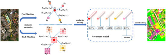
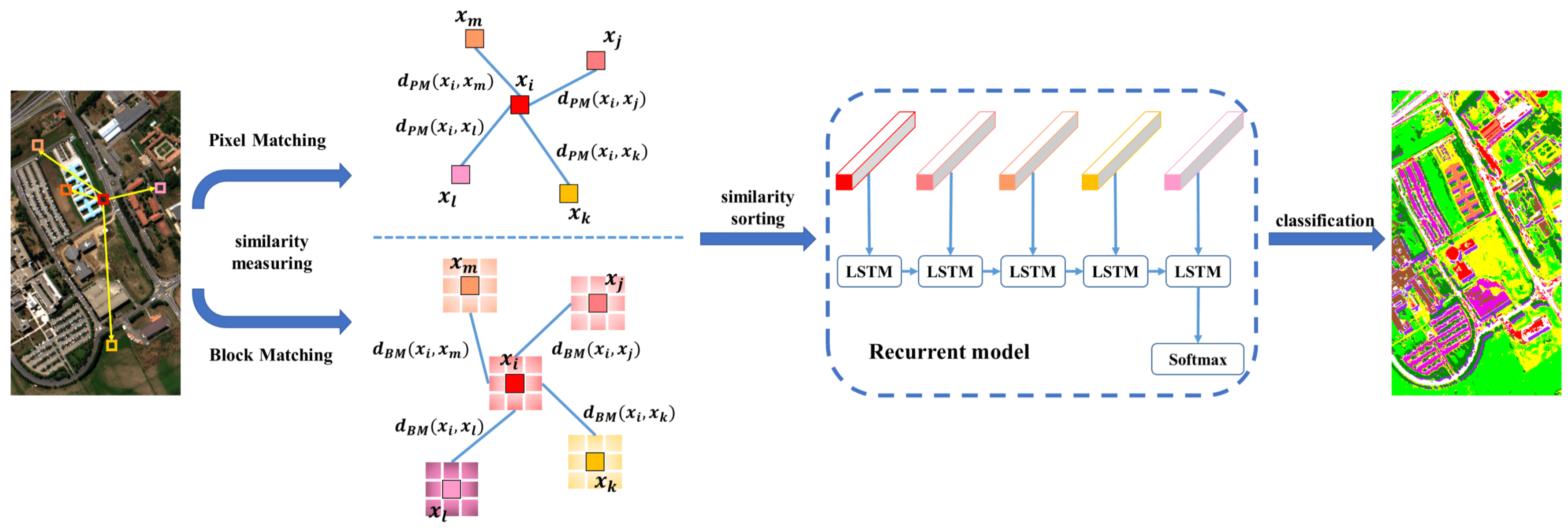
In this paper, we propose a novel LSTM-based HSI classification framework with spatial similarity measurements (SSM), which is inspired by [47], where the LSTM model and the spatial location are combined simultaneously. First, the sequential feature for each pixel is constructed by selecting candidates from the whole image based on the similarity between each candidate and the target pixel. This selection method mainly relies upon two different similarity measurements where spectral and spatial information are considered, namely pixel-matching-based (PM) spatial similarity measurements and block-matching-based (BM) spatial similarity measurements, respectively. LSTM entails the significant capability of handling sequential data, and it achieves outstanding performance in NLP. The proposed similarity-measuring strategies provide an innovative framework to extract sequential features for HSI classification by employing all pixels in the entire HSI, regardless of whether the pixel candidates to be a given sequential feature are labeled or not. The proposed sequential feature effectively encodes the dependency of the target pixel with regard to its contexts, where the pixel-level spectral similarities and the patch-, or block-level contextual similarities are naturally encoded, respectively. More specifically, LSTM assumes that closer “time steps” (which denote selected pixels/blocks with higher similarity) in general have stronger feature sharing, while also allowing for longer-term dependency that can account for non-local similarity and long-tail effects. The motivation for extending one pixel to its sequential features is essentially to find a new feature embedding of the pixel, which makes reference to other similar pixels. The action of re-ordering those pixels in terms of their similarity measures is to ensure that all obtained sequential features admit “comparable” formats in terms of monotonically-decreasing similarity to the original pixel (i.e., the target pixel, or the given pixel of interest). In this framework, the influence of unlabeled data in an HSI is enhanced compared with conventional supervised-learning methods due to our proposed spatial selection, where any pixel can be selected as a candidate to construct sequential features. In view of global searching based on the whole image, more supportive pixels are incorporated with a wider receptive domain. In addition, spatial contextual information, which has already been utilized to reduce the “salt-and-pepper” phenomenon in remote-sensing/HSI classification [48], is also investigated here in the BM-based framework. Similarity measurements of two pixels is implemented by using the neighboring points of two pixels instead of their spectral feature vectors. Compared with the PM-based method, the BM-based scheme can obtain more typical sequential feature representation combining both spectral and spatial features together. In summary, this is the first study to propose such methods operating over the entire image. This is important because these new, novel methods can incorporate additional information collected throughout the whole image by exploiting unlabeled pixels, instead of utilizing only the limited prior information in the form of labeled pixels. Figure 1 illustrates the framework of our proposed method.

The organization of the remainder of this paper is as follows: Section 2 provides a brief introduction to the original RNN and LSTM models. Section 3 describes the proposed LSTM classification framework based on pixel matching and block matching. Experimental results are discussed in Section 4. Section 5 presents the conclusions.

2. Background: RNN and LSTM

2.1. RNN

The recurrent neural network (RNN) has shown great capability in time-sequence data processing, including NLP [49] and speech recognition [40]. A significant characteristic of a time sequence is that there is typically a strong relationship between a given sample and the previous samples. In the hidden Markov model (HMM), which is a widely-utilized sequence model in language processing, the probability of a specific state depends only on its previous state, instead of all previous states. Let $\mathbf{X}=[{\mathbf{x}}_{\mathbf{1}},{\mathbf{x}}_{\mathbf{2}},\cdots ,{\mathbf{x}}_{\mathbf{t}}]$ be the sequence data where t is the label of state. ${\mathbf{x}}_{\mathbf{1}}$ represents the data at the first state, and ${\mathbf{x}}_{\mathbf{t}}$ represents the data at the t state. The Markov assumption can be formulated as

$$P\left({\mathbf{x}}_{\mathbf{t}}\right|{\mathbf{x}}_{\mathbf{1}},\cdots ,{\mathbf{x}}_{\mathbf{t}-\mathbf{1}})=P\left({\mathbf{x}}_{\mathbf{t}}\right|{\mathbf{x}}_{\mathbf{t}-\mathbf{1}}),$$

(1)

where $P(·)$ expresses the conditional probability. Compared with HMM, RNN is quite similar with HMM since the computation on the current state relies on the previous state. In contrast to conventional ANNs, the RNN has a circular processing on the sequential data, which means that such processing will be applied on each data instance in the sequence, and the result at each state relies on the previous state. This circular processing also represents the parameter sharing. Parameter sharing is a prevalent method to control the number of parameters in a DL scheme. Still given $\mathbf{X}=[{\mathbf{x}}_{\mathbf{1}},{\mathbf{x}}_{\mathbf{2}},\cdots ,{\mathbf{x}}_{\mathbf{t}}]$ as sequential data, the hidden state ${\mathbf{s}}_{\mathbf{t}}$ can be represented as

$${\mathbf{s}}_{\mathbf{t}}=f_s({\mathbf{W}}_{\mathbf{xs}}{\mathbf{x}}_{\mathbf{t}}+{\mathbf{W}}_{\mathbf{ss}}{\mathbf{s}}_{\mathbf{t}-\mathbf{1}}+{\mathbf{b}}_{\mathbf{t}}),$$

(2)

where ${\mathbf{W}}_{\mathbf{xs}}$ is the weight matrix from input data to the hidden state, and ${\mathbf{W}}_{\mathbf{ss}}$ is the weight matrix from the current state to the next state, respectively. ${\mathbf{b}}_{\mathbf{t}}$ is the bias variable. ${\mathbf{s}}_{\mathbf{t}}$ denotes the hidden state at time step t, and $f_s(·)$ represents the nonlinear activation function. The calculation of the output at state t is quite similar with Equation (2) as follows:

$${\mathbf{y}}_{\mathbf{t}}=f_y({\mathbf{W}}_{\mathbf{sy}}{\mathbf{s}}_{\mathbf{t}}+{\mathbf{b}}_{\mathbf{y}}),$$

(3)

where ${\mathbf{W}}_{\mathbf{sy}}$ is the weight matrix from the hidden state to the output. ${\mathbf{b}}_{\mathbf{y}}$ is the bias, and $f_y(·)$ is the nonlinear activation function.

The hidden state ${\mathbf{s}}_{\mathbf{t}}$ can be viewed as the memory of the RNN model, as it is calculated based on the previous state through forward propagation. Meanwhile, sequential data in the previous states are taken into consideration as well. In such forward propagation, some parameters, including three different weight matrices ${\mathbf{W}}_{\mathbf{xs}}$, ${\mathbf{W}}_{\mathbf{ss}}$, and ${\mathbf{W}}_{\mathbf{sy}}$, are shared across all steps, which is quite different from a traditional neural network. The parameter-sharing scheme reduces the number of trainable parameters, and makes the total computation more efficient.

2.2. LSTM

In Equation (2), the calculation of the hidden state depends on the previous state. However, with the increase in the length of the sequence data, gradient vanishing and gradient exploding will be introduced in this recurrent model due to the forward and backward propagations of weight matrices. To address this issue, long short-term memory was developed with a more sophisticated recurrent neuron. In LSTM, each recurrent neuron can be regarded as a cell state. Similar to the conventional RNN, LSTM also employs the previous state as the input to the current state. However, with LSTM, there are three gates, including forget gate, update gate, and output gate, to control the update of the current neuron. Figure 2 illustrates the basic structure of the LSTM recurrent unit.

The first part of LSTM is the forget gate which determines if the previous state will be retained or not. Still given $\mathbf{X}=[{\mathbf{x}}_{\mathbf{1}},{\mathbf{x}}_{\mathbf{2}},\cdots ,{\mathbf{x}}_{\mathbf{t}}]$ as sequential data, ${\mathbf{y}}_{\mathbf{t}}$ and ${\mathbf{s}}_{\mathbf{t}}$ are the output and the hidden state at step t, respectively. The common computation for forget gate ${\mathbf{f}}_{\mathbf{t}}$ is as follows:

$${\mathbf{f}}_{\mathbf{t}}={\sigma }_f({\mathbf{W}}_{\mathbf{yf}}{\mathbf{y}}_{\mathbf{t}-\mathbf{1}}+{\mathbf{W}}_{\mathbf{xf}}{\mathbf{x}}_{\mathbf{t}}+{\mathbf{b}}_{\mathbf{f}}),$$

(4)

where the ${\mathbf{W}}_{(·)}$ terms denote the weight matrices, and the ${\mathbf{b}}_{(·)}$ term is the bias variable. $\sigma (·)$ is the logistic sigmoid function. The following step is to compute the update gate ${\mathbf{u}}_{\mathbf{t}}$ and a new candidate state value $\widetilde{{\mathbf{s}}_{\mathbf{t}}}$:

$${\mathbf{u}}_{\mathbf{t}}={\sigma }_u({\mathbf{W}}_{\mathbf{yu}}{\mathbf{y}}_{\mathbf{t}-\mathbf{1}}+{\mathbf{W}}_{\mathbf{xu}}{\mathbf{x}}_{\mathbf{t}}+{\mathbf{b}}_{\mathbf{u}}),$$

(5)

$$\widetilde{{\mathbf{s}}_{\mathbf{t}}}=tanh({\mathbf{W}}_{\mathbf{ys}}{\mathbf{y}}_{\mathbf{t}-\mathbf{1}}+{\mathbf{W}}_{\mathbf{xs}}{\mathbf{x}}_{\mathbf{t}}+{\mathbf{b}}_{\mathbf{s}}),$$

(6)

where $tanh(·)$ is the hyperbolic tangent function. Then, the new hidden step ${\mathbf{s}}_{\mathbf{t}}$ can be updated by using the aforementioned equations

$${\mathbf{s}}_{\mathbf{t}}={\mathbf{s}}_{\mathbf{t}-\mathbf{1}}\times {\mathbf{f}}_{\mathbf{t}}+\widetilde{{\mathbf{s}}_{\mathbf{t}}}\times {\mathbf{u}}_{\mathbf{t}}.$$

(7)

Finally, the output gate and the output of the current neuron yields:

$${\mathbf{o}}_{\mathbf{t}}={\sigma }_o({\mathbf{W}}_{\mathbf{yo}}{\mathbf{y}}_{\mathbf{t}-\mathbf{1}}+{\mathbf{W}}_{\mathbf{xo}}{\mathbf{x}}_{\mathbf{t}}+{\mathbf{b}}_{\mathbf{o}}),$$

(8)

$${\mathbf{y}}_{\mathbf{t}}={\mathbf{o}}_{\mathbf{t}}\times tanh\left({\mathbf{s}}_{\mathbf{t}}\right).$$

(9)

3. Spatial Similarity Measurements in LSTM

For the LSTM model, the sequential feature is a critical issue when training LSTM since determining the representative feature will improve classification performance and reduce the training-time cost. In this section, the spatial similarity measurement-based LSTM model will be introduced as a method to construct sequential features. First, two different strategies utilized in SSM will be discussed, named PM-based and BM-based schemes. For each of them, when computing the similarity between pixels, two distance measurements are investigated, which are Euclidean distance (EU) and spectral angle mapper (SAM). Furthermore, we will introduce the way of constructing sequence as the input of LSTM model.

3.1. Pixel Matching

Measuring the similarity in the pixel data vectors between different pixels is a common technology in many HSI analysis applications, such as endmember-based analysis [50], manifold learning [51,52], and graph-based semi-supervised learning [22]. Since HSIs have abundant spectral information, typically entailing hundreds of bands, spectral features collected from all bands have the most discriminative capability to distinguish different ground objects or materials encompassed within the given image, and have been most widely utilized in HSI classification [53]. In the pixel-matching scheme, pairwise spectral similarity measurements are applied for all pixels. Suppose we have HSI data $\mathbf{X}\in {\mathbb{R}}^{L\times C\times B}$ with L rows, C columns, and B bands. $\mathbf{X}$ can be rewritten as $\mathbf{X}=[{\mathbf{x}}_{\mathbf{1}},{\mathbf{x}}_{\mathbf{2}},...,{\mathbf{x}}_{\mathbf{N}}]\in {\mathbb{R}}^{B\times N}$ with row-major order, where N is the total number of pixels in the HSI, which equals $L\ast C$. For any pixels ${\mathbf{x}}_{\mathbf{i}}$ in $\mathbf{X}$, the distances measured between ${\mathbf{x}}_{\mathbf{i}}$ and all pixels of $\mathbf{X}$ will be computed as follows:

$$d_{\mathrm{PM}}({\mathbf{x}}_{\mathbf{i}},\mathbf{X})=[d({\mathbf{x}}_{\mathbf{i}},{\mathbf{x}}_{\mathbf{1}}),\cdots ,d({\mathbf{x}}_{\mathbf{i}},{\mathbf{x}}_{\mathbf{j}}),\cdots ,d({\mathbf{x}}_{\mathbf{i}},{\mathbf{x}}_{\mathbf{N}})],$$

(10)

where $d({\mathbf{x}}_{\mathbf{i}},{\mathbf{x}}_{\mathbf{j}})$ denotes the distance between ${\mathbf{x}}_{\mathbf{i}}$ and ${\mathbf{x}}_{\mathbf{j}}$, and $d(·)$ is the distance calculation function. There are multiple methods available to compute pairwise distance. In this paper, Euclidean distance and the spectral angle mapper (SAM) are utilized in the pixel-matching scheme. Euclidean distance is a well-known distance measurement, and its definition is given as follows:

$$d_{\mathrm{EU}}({\mathbf{x}}_{\mathbf{i}},{\mathbf{x}}_{\mathbf{j}})=\sqrt{{(x_i^1-x_j^1)}^2+{(x_i^2-x_j^2)}^2+\dots +{(x_i^B-x_j^B)}^2}=\parallel {\mathbf{x}}_{\mathbf{i}}-{\mathbf{x}}_{\mathbf{j}}\parallel .$$

(11)

The other distance measure adopted in this study is SAM, which is investigated well in endmember-based HSI classification. It can be defined as follows:

$$d_{\mathrm{SAM}}({\mathbf{x}}_{\mathbf{i}},{\mathbf{x}}_{\mathbf{j}})={cos}^{-1}(\frac{{\mathbf{x}}_{\mathbf{i}}{}^{\mathrm{T}}{\mathbf{x}}_{\mathbf{j}}}{\parallel {\mathbf{x}}_{\mathbf{i}}\parallel \parallel {\mathbf{x}}_{\mathbf{j}}\parallel }).$$

(12)

In the following text of this paper, we use $d_{(·)}\left(\right)$ to represent either the EU or SAM distance calculation function in the pixel-wise measurement. Therefore, Equation (10) can be rewritten as follows:

$$d_{\mathrm{PM}}({\mathbf{x}}_{\mathbf{i}},\mathbf{X})=[d_{(·)}({\mathbf{x}}_{\mathbf{i}},{\mathbf{x}}_{\mathbf{1}}),\cdots ,d_{(·)}({\mathbf{x}}_{\mathbf{i}},{\mathbf{x}}_{\mathbf{j}}),\cdots ,d_{(·)}({\mathbf{x}}_{\mathbf{i}},{\mathbf{x}}_{\mathbf{N}})].$$

(13)

3.2. Block Matching

Although spectral features provide rich, significant information that facilitates discrimination of different ground objects in HSI, classification accuracy based on utilization of spectral features alone is not always satisfactory due to the “salt-and-pepper” phenomenon [48]. Given Tobler’s First Law of Geography [54], incorporation of spatial contextual information has attracted increasing attention in the research literature in recent years and has exhibited the capability to reduce “salt-and-pepper” noise and improve classification performance, including yielding smoother classification maps. In the current study, we utilize the image patch distance (IPD), proposed in [55], for similarity measurement that considers local spatial information. The IPD method was developed based on the Hausdorff distance [56], also referred to as the Pompeiu–Hausdorff distance. Instead of using spectral features to measure the pairwise similarity between two pixels, spatial neighbors within the respective local window of such two pixels will also be employed. Let w be the local window size, and the ${\mathbf{s}}_{\mathbf{i}}$ represents the block neighborhood, where pixel ${\mathbf{x}}_{\mathbf{i}}$ is centered within the $w\times w$ spatial window. All block sets $\mathbf{S}$ can be defined as follows:

$$\mathbf{S}=[{\mathbf{s}}_{\mathbf{1}},{\mathbf{s}}_{\mathbf{2}},\cdots ,{\mathbf{s}}_{\mathbf{N}}].$$

(14)

Given $\forall {\mathbf{s}}_{\mathbf{i}},{\mathbf{s}}_{\mathbf{j}}\in \mathbf{S}$, we first calculate the distances between one arbitrary pixel ${\mathbf{x}}_{\mathbf{m}}$ from ${\mathbf{s}}_{\mathbf{i}}$ and ${\mathbf{s}}_{\mathbf{j}}$ and then select the minimum distance as follows:

$$d_{min}({\mathbf{x}}_{\mathbf{m}},{\mathbf{s}}_{\mathbf{j}})=\underset{{\mathbf{x}}_{\mathbf{n}}\in {\mathbf{s}}_{\mathbf{j}}}{min}{d}_{(·)}({\mathbf{x}}_{\mathbf{m}},{\mathbf{x}}_{\mathbf{n}}),$$

(15)

where $d(·)$ is the distance-measuring function. Correspondingly, the minimum distance between one arbitrary pixel ${\mathbf{x}}_{\mathbf{m}}$ from ${\mathbf{s}}_{\mathbf{j}}$ and ${\mathbf{s}}_{\mathbf{i}}$ can be computed in the following manner:

$$d_{min}({\mathbf{x}}_{\mathbf{m}},{\mathbf{s}}_{\mathbf{i}})=\underset{{\mathbf{x}}_{\mathbf{n}}\in {\mathbf{s}}_{\mathbf{i}}}{min}{d}_{(·)}({\mathbf{x}}_{\mathbf{m}},{\mathbf{x}}_{\mathbf{n}}).$$

(16)

Therefore, the definition of block matching between ${\mathbf{s}}_{\mathbf{i}}$ and ${\mathbf{s}}_{\mathbf{j}}$ is:

$$\begin{array}{cc}\hfill d_{\mathrm{BM}}({\mathbf{s}}_{\mathbf{i}},{\mathbf{s}}_{\mathbf{j}})& =\sum _{m=1}^{w^2}(max(d_{min}({\mathbf{x}}_{\mathbf{m}},{\mathbf{s}}_{\mathbf{i}}),d_{min}({\mathbf{x}}_{\mathbf{m}},{\mathbf{s}}_{\mathbf{i}})))\hfill \\ & =\sum _{m=1}^{w^2}(max(\underset{{\mathbf{x}}_{\mathbf{n}}\in {\mathbf{s}}_{\mathbf{j}}}{min}{d}_{(·)}({\mathbf{x}}_{\mathbf{m}},{\mathbf{x}}_{\mathbf{n}}),\underset{{\mathbf{x}}_{\mathbf{n}}\in {\mathbf{s}}_{\mathbf{i}}}{min}{d}_{(·)}({\mathbf{x}}_{\mathbf{m}},{\mathbf{x}}_{\mathbf{n}}))).\hfill \end{array}$$

(17)

Finally, the ultimate BM measurements are defined as:

$$\begin{array}{cc}\hfill d_{\mathrm{BM}}({\mathbf{x}}_{\mathbf{i}},\mathbf{X})& =d_{\mathrm{BM}}({\mathbf{s}}_{\mathbf{i}},\mathbf{X})\hfill \\ & =[d_{\mathrm{BM}}({\mathbf{s}}_{\mathbf{i}},{\mathbf{s}}_{\mathbf{1}}),\cdots ,d_{\mathrm{BM}}({\mathbf{s}}_{\mathbf{i}},{\mathbf{s}}_{\mathbf{j}}),\cdots ,d_{\mathrm{BM}}({\mathbf{s}}_{\mathbf{i}},{\mathbf{s}}_{\mathbf{N}})].\hfill \end{array}$$

(18)

3.3. Sequential Feature Extraction

After measuring the pairwise similarity among pixels in the whole image, the sequential feature for each pixel is extracted so that it can be fed into the RNN model directly. Based on the aforementioned two matching schemes, given one pixel ${\mathbf{x}}_{\mathbf{i}}\in \mathbf{X}$, its corresponding matching vector is

$$d_M({\mathbf{x}}_{\mathbf{i}},\mathbf{X})=[d_M({\mathbf{x}}_{\mathbf{i}},{\mathbf{x}}_{\mathbf{1}}),\cdots ,d_M({\mathbf{x}}_{\mathbf{i}},{\mathbf{x}}_{\mathbf{j}}),\cdots ,d_M({\mathbf{x}}_{\mathbf{i}},{\mathbf{x}}_{\mathbf{N}})],$$

(19)

where $d_M(·)$ denotes the pairwise matching function introduced in previous sections. Note that the order of $d_M({\mathbf{x}}_{\mathbf{i}},\mathbf{X})$ is determined only based on its location in the image. To characterize a representative sequential feature, $d_M(·)$ is reordered based on the degree of similarity, and then the corresponding pixels are selected as the sequential representation. With the definition given in Equation (19), we assume we have one pixel ${\mathbf{x}}_{\mathbf{i}}\in \mathbf{X}$, its reordered $d_M({\mathbf{x}}_{\mathbf{i}},\mathbf{X})$, named $d_{sf}({\mathbf{x}}_{\mathbf{i}},\mathbf{X})$, is built as follows:

$$d_{sf}({\mathbf{x}}_{\mathbf{i}},\mathbf{X})=[d_{sf}^{i1},\cdots ,d_{sf}^{ij},\cdots ,d_{sf}^{iN}],$$

(20)

where $d_{sf}^{ij}$ denotes the distance-measuring result between ${\mathbf{x}}_{\mathbf{i}}$ and ${\mathbf{x}}_{\mathbf{j}}$. $d_{sf}({\mathbf{x}}_{\mathbf{i}},\mathbf{X})$ is the ascending sort of $d_M({\mathbf{x}}_{\mathbf{i}},\mathbf{X})$. More specifically, $d_{sf}^1$ is the minimum value among $d_{sf}({\mathbf{x}}_{\mathbf{i}},\mathbf{X})$, and $d_{sf}^2$ is the second-smallest value. During ascending sorting, pixels most similar to ${\mathbf{x}}_{\mathbf{i}}$ among all pixels in the whole image will be selected as the sequential representation of ${\mathbf{x}}_{\mathbf{i}}$. Note that not all candidates in $d_{sf}({\mathbf{x}}_{\mathbf{i}},\mathbf{X})$ will be considered, and the parameter l is defined to control how many candidates can be selected or to determine the length of such sequence. The first l pixels with distance-measuring results from $d_{sf}^1$ to $d_{sf}^l$ will be selected, and the first elements of this sequence is ${\mathbf{x}}_{\mathbf{i}}$ itself since $d_M({\mathbf{x}}_{\mathbf{i}},{\mathbf{x}}_{\mathbf{i}})$ equals zero, which is the minimum value in $d_M({\mathbf{x}}_{\mathbf{i}},\mathbf{X})$. Given the sequence length l, the final sequential feature of ${\mathbf{x}}_{\mathbf{i}}$ can be defined:

$$d_{sf}\left({\mathbf{x}}_{\mathbf{i}}\right)=[{\mathbf{x}}_{\mathbf{sf}}^{\mathbf{i}\mathbf{1}},\cdots ,{\mathbf{x}}_{\mathbf{sf}}^{\mathbf{ij}},\cdots ,{\mathbf{x}}_{\mathbf{sf}}^{\mathbf{il}}],$$

(21)

where ${\mathbf{x}}_{\mathbf{sf}}^{\mathbf{ij}}$ represents ${\mathbf{x}}_{\mathbf{j}}$, whose distance-measuring result is located at the jth place.

4. Experimental Setup, Results, and Discussion

4.1. Datasets

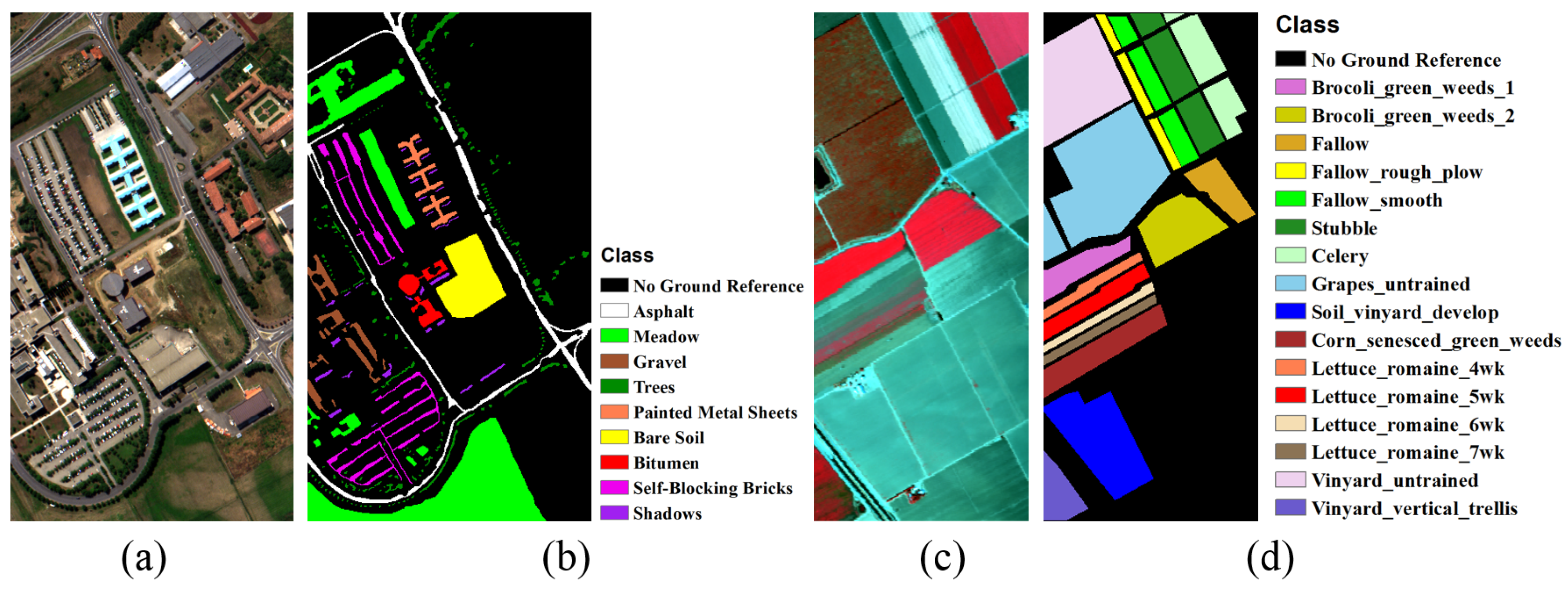
In this study, two benchmark HSI datasets were utilized, including Pavia University, and Salinas images, as displayed in Figure 3 and

Table 1. Class codes for Pavia University and Salinas images.

Pavia University Image		Salinas image
Class No.	Name	Class No.	Name
1	Asphalt	1	Brocoli_green_weeds_1
2	Meadow	2	Brocoli_green_weeds_2
3	Gravel	3	Fallow
4	Trees	4	Fallow_rough_plow
5	Painted Metal Sheets	5	Fallow_smooth
6	Bare Soil	6	Stubble
7	Bitumen	7	Celery
8	Self-Blocking Bricks	8	Grapes_untrained
9	Shadows	9	Soil_vinyard_develop
		10	Corn_senesced_green_weeds
		11	Lettuce_romaine_4wk
		12	Lettuce_romaine_5wk
		13	Lettuce_romaine_6wk
		14	Lettuce_romaine_7wk
		15	Vinyard_untrained
		16	Vinyard_vertical_trellis

. The Pavia University image was collected by the Reflective Optics System Imaging Spectrometer (ROSIS) sensor. It consists of 102 spectral bands, with a spectral range from 430 nm to 860 nm. The image spatial resolution is 1.3 m, and the total image size is 610 × 340 pixels. For the Pavia University image extent, nine (9) classes were considered in the classification experiments. The Salinas image was acquired via the Airborne Visible/Infrared Imaging Spectrometer (AVIRIS), and the image contains 512 lines × 217 samples, with the spatial resolution of 3.7 m. After removing 20 noise and water-absorption bands, 204 spectral bands remained for subsequent analysis. The ground-reference data for the Salinas image entails 16 classes.

4.2. Experimental Design

To evaluate the performance of the proposed SSM-based LSTM methods, three algorithms, including SVM, 1DCNN [35], and 1DLSTM [44], are investigated as baseline algorithms. For SVM, the radial basis function (RBF) is utilized as kernel function, and the parameters of SVM are acquired by cross validation. For the following two deep-learning algorithms, they are 1D-based architectures, where spectral features are fed into the classifier directly. For the 1DCNN, two convolutional layers, two max pooling layers, and one fully-connected (FC) layer are selected due to the limited available training samples. For the 1DLSTM architecture, three LSTM layers and one FC layer are adopted. Different model structures are implemented based on different images, and the specific parameter settings for the Pavia Univeristy and Salinas images are summarized in

Table 2. Parameter settings for 1D-CNN and 1D-LSTM, where the convolutional layer is represented as “Conv(number of kernels)-(kernel size)”, maxpooling layer is performed as “Maxpooling-(kernel size)”, and LSTM layer is denoted as “LSTM-(kernel size)”.

Pavia University Image		Salinas Image
1DCNN	1DLSTM	1DCNN	1DLSTM
Conv(10)-8	LSTM-32	Conv(8)-12	LSTM-32
Maxpooling-2	LSTM-64	Maxpooling-2	LSTM-64
Conv(10)-8	LSTM-128	Conv(8)-12	LSTM-128
Maxpooling-2		Maxpooling-2
FC layer-9		FC layer-16

, where the convolutional layer is represented as “Conv(number of kernels)-(kernel size)”, maxpooling layer is performed as “Maxpooling-(kernel size)”, and LSTM layer is denoted as “LSTM-(kernel size)”. Regarding the proposed methods, both pixel-matching and block-matching are investigated, and, for each matching scheme, EU and SAM are employed as distance measurements. Therefore, there are four different LSTM-based classification frameworks investigated here, named LSTM_PM_EU, LSTM_PM_SAM, LSTM_BM_EU, and LSTM_BM_SAM. For the LSTM structure, we use four recurrent layers and two fully-connected layers, and the length of the sequential feature is 20. The size of the recurrent layers are 32, 64, 128, and 256, respectively, and the size of first fully-connected layer is 50. The second fully-connected layer is applied for the purpose of classification, and its length equals the number of classes. During training of the recurrent model, the batch size is set to 20, and the number of epochs is 500.

In order to evaluate classification performance quantitatively, all ground-reference data for each image is randomly split into training and testing sample sets. In our experiments, we randomly select 200 samples per class as training data, with the remaining ground-reference data used as testing data. Ten replications of the experiments with such random selections were performed, and all classification accuracies were averaged across the ten replications. Furthermore, three other quantitative indicators were also adopted for the evaluation, including overall accuracy (OA), average accuracy (AA), and the Kappa coefficient (Kappa) [57]. The pixel-matching and block-matching experiments were implemented on the Texas A&M High Performance Research Computing (HPRC) system, and the remaining experiments, such as training LSTM models and classification accuracy assessments, were carried out on a local workstation with a 3.2 GHz Intel(R) core i7-8700 Central Processing Unit (CPU), and a NVIDIA(R) GeForce GTX 1070 graphics card.

4.3. Classification Results: Pavia University Image

The first set of experiments is conducted on the Pavia University image. The quantitative results are shown in

Table 3. Comparison of different classification accuracy results for the Pavia University image (%), where LSTM_PEU equals LSTM_PM_EU, LSTM_PSAM equals LSTM_PM_SAM, LSTM_BEU equals LSTM_BM_EU, and LSTM_BSAM equals LSTM_BM_SAM.

Class No.	SVM	1DCNN	1DLSTM	LSTM_PEU	LSTM_PSAM	LSTM_BEU	LSTM_BSAM
1	97.52 ± 0.21	96.53 ± 0.57	95.76 ± 0.65	85.51 ± 3.06	94.06 ± 0.72	98.76 ± 0.44	98.78 ± 0.39
2	95.77 ± 0.30	94.78 ± 1.55	94.13 ± 0.93	94.11 ± 1.40	96.01 ± 1.08	99.08 ± 0.25	98.84 ± 0.29
3	65.57 ± 3.41	68.93 ± 3.65	64.29 ± 3.02	70.41 ± 2.27	66.61 ± 3.68	90.22 ± 2.28	89.22 ± 2.63
4	71.27 ± 7.38	76.62 ± 7.92	75.71 ± 4.95	62.69 ± 6.28	81.58 ± 4.77	92.97 ± 2.19	94.70 ± 1.71
5	95.50 ± 1.55	98.50 ± 0.86	97.73 ± 1.31	98.51 ± 0.67	95.57 ± 2.80	98.99 ± 1.18	99.42 ± 0.64
6	59.51 ± 6.74	63.62 ± 11.03	61.12 ± 7.62	69.71 ± 8.18	64.39 ± 8.23	88.65 ± 4.93	90.65 ± 3.92
7	52.10 ± 0.93	66.87 ± 4.86	65.74 ± 3.62	63.76 ± 4.45	56.69 ± 4.42	89.72 ± 4.25	88.47 ± 6.60
8	84.27 ± 1.13	83.54 ± 1.73	81.48 ± 1.70	82.37 ± 1.59	80.50 ±  1.01	93.32 ± 2.46	93.27 ± 1.28
9	99.92 ± 0.11	99.65 ± 0.31	99.72 ± 0.35	93.74 ± 2.05	95.99 ± 5.06	99.09 ± 0.62	98.49 ± 1.75
OA	82.12 ± 1.79	84.45 ± 3.01	83.41 ± 2.66	82.70 ± 1.73	84.56 ± 2.41	95.96 ± 1.01	96.20 ± 0.57
AA	80.16 ± 0.96	83.23 ± 1.71	81.74 ± 1.47	80.09 ± 1.19	81.27 ± 1.72	94.53 ± 0.98	94.65 ± 0.64
Kappa	76.98 ± 2.12	79.79 ± 3.53	78.42 ± 3.13	77.40 ± 2.05	79.86 ± 2.89	94.60 ± 1.31	94.91 ± 0.75

, where values in bold are the highest class-specific accuracies and the standard deviations are also presented, which are calculated based on ten OAs obtained from the aforementioned ten (10) experimental replications. The classified images are displayed in Figure 4 for qualitative analysis, which are obtained from the fifth trial. As shown in Table 3, the block-matching-based method LSTM_BM_SAM achieved best performance, with 96.20% OA, 94.65% AA, and 94.91% Kappa. For the first three benchmark algorithms, the highest OA (i.e., 84.45%) is obtained from 1DCNN. Regarding our newly-proposed pixel-matching-based LSTM frameworks, the OA of LSTM_PM_SAM is 84.56%, exhibiting limited improvement relative to SVM, 1DCNN, and 1DLSTM, and the classification performance of LSTM_PM_EU even decreases relative to 1DCNN and 1DLSTM. However, after incorporating spatial information via similarity measurements, LSTM_BM_EU and LSTM_BM_SAM obtain marked improvements over all non-block-matching methods, with 95.96% and 96.20% OA, respectively. Within each matching method, the performance of SAM is always better than that of the Euclidean distance. Regarding the AA of each class, class 7 (Bitumen, Red) is more difficult to discriminate compared with other classes due to the mixed spectral features. The proposed LSTM_BM_SAM improves the original SVM OA by more than 35%.

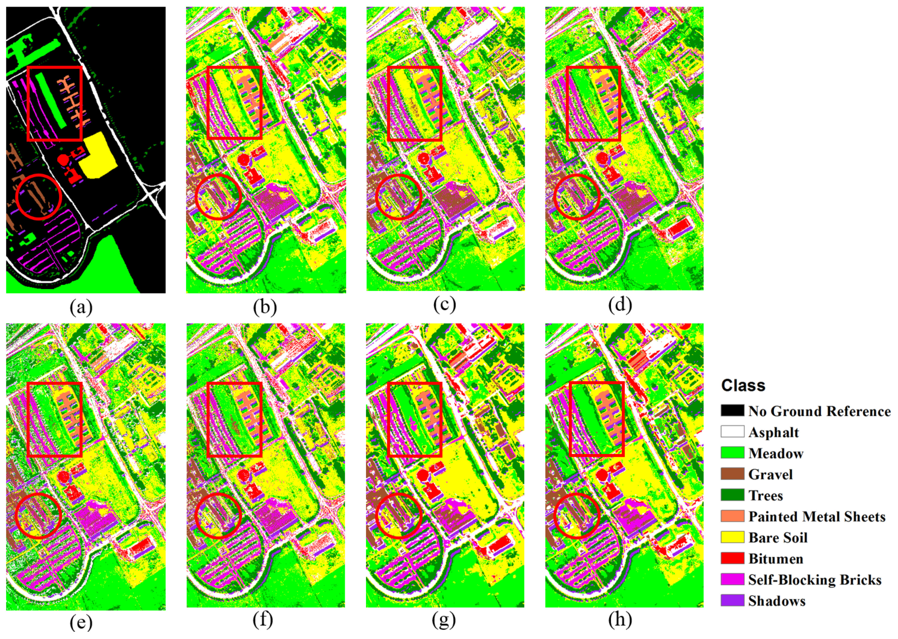
From the classification maps shown in Figure 4, marked improvements in classification performance are visually apparent. In Figure 4b–f, “salt-and-pepper” noise is still obvious due to the lack of incorporation of spatial contextual information in the classification. Within the red-rectangle annotation, many class 2 (Meadow, Bright Green) pixels are misclassified as class 6 (Bare Soil, Yellow), and class 3 (Gravel, Brown), as shown in Figure 4b–f. However, the classification maps derived from LSTM_BM_EU and LSTM_BM_SAM (Figure 4g,h) are spatially smooth and generally correctly classified, where most discrete, spurious/misclassified points are eliminated if they are located within an otherwise homogeneous area. Therefore, combining spatial contextual information can yield marked alleviation of image misclassification. Similar to what is observed within the red-rectangle annotation, more accurate and homogeneous classification results can be achieved within the red-circle annotation as well. Such results demonstrate the validity and capability of combining spatial and spectral features together when measuring the similarity between two pixels, and the effectiveness of constructing a sequential feature for a specific pixel based on such similarity between that target pixel itself and candidates from the whole image.

4.4. Classification Results: Salinas Image

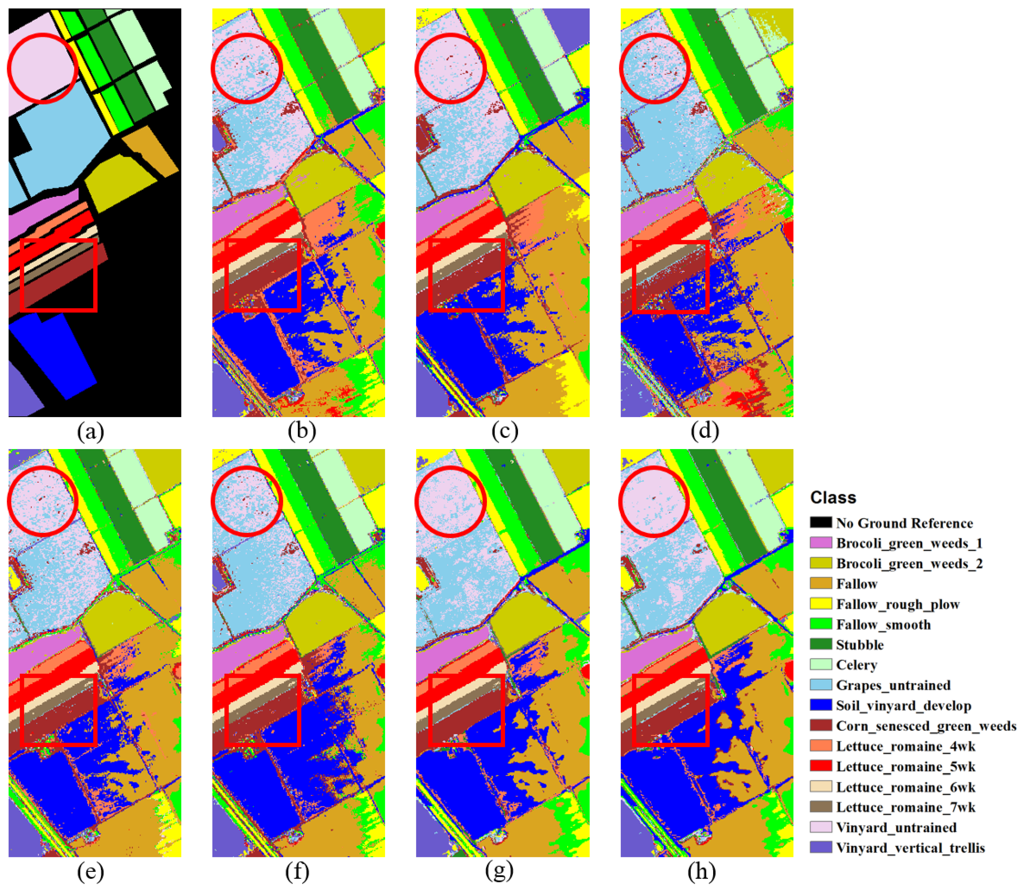
For the Salinas image, the results are similar to those attained and described in Section 4.3. The quantitative results are shown in

Table 4. Comparison of different classification results for the Salinas image (%), where LSTM_PEU equals LSTM_PM_EU, LSTM_PSAM equals LSTM_PM_SAM, LSTM_BEU equals LSTM_BM_EU, and LSTM_BSAM equals LSTM_BM_SAM.

Class No.	SVM	1DCNN	1DLSTM	LSTM_PEU	LSTM_PSAM	LSTM_BEU	LSTM_BSAM
1	96.84 ± 1.18	99.12 ± 1.52	94.18 ± 10.04	98.61 ± 3.93	99.40 ± 0.89	95.78 ± 11.30	99.86 ± 0.22
2	98.79 ± 0.13	98.79 ± 0.69	98.69 ± 0.78	98.75 ± 1.08	99.39 ± 0.28	99.60 ± 0.16	99.34 ± 0.51
3	85.11 ± 1.38	95.53 ± 1.32	88.68 ± 7.32	92.89 ± 3.68	95.70 ± 1.07	96.11 ± 1.25	96.24 ± 1.10
4	97.44 ± 0.18	97.94 ± 0.67	97.20 ± 1.02	98.33 ± 0.74	98.45 ± 0.68	98.66 ± 0.95	97.90 ± 1.70
5	95.03 ± 0.85	97.20 ± 2.76	98.07 ± 1.65	96.26 ± 7.50	97.63 ± 1.57	98.75 ± 1.65	98.83 ± 0.68
6	99.79 ± 0.11	99.77 ± 0.21	98.98 ± 1.16	99.64 ± 0.44	99.45 ± 0.87	99.69 ± 0.36	99.71 ± 0.33
7	98.63 ± 0.44	99.35 ± 0.62	98.81 ± 0.91	99.37 ± 0.53	99.11 ± 0.76	99.40 ± 0.43	99.38 ± 0.51
8	76.70 ± 1.31	83.99 ± 4.02	76.24 ± 5.90	76.97 ± 2.91	76.50 ± 3.48	83.04 ± 1.37	85.66 ± 3.00
9	99.12 ± 0.04	99.02 ± 0.29	98.03 ± 1.46	98.78 ± 0.28	98.66 ± 0.33	99.20 ± 0.41	99.43 ± 0.27
10	81.91 ± 1.58	85.89 ± 2.09	84.90 ± 1.94	85.94 ± 4.19	88.65 ± 1.20	94.16 ± 1.58	91.00 ± 2.13
11	69.51 ± 1.00	82.23 ± 6.71	81.23 ± 13.79	76.81 ± 8.06	83.24 ± 4.33	86.00 ± 3.27	83.49 ± 4.40
12	93.33 ± 0.34	96.82 ± 1.05	87.58 ± 9.57	97.09 ± 1.33	97.26 ± 1.03	98.31 ± 1.36	98.26 ± 1.67
13	92.67 ± 0.65	94.15 ± 2.62	90.12 ± 4.05	96.07 ± 2.23	95.27 ± 2.27	95.89 ± 2.78	97.33 ± 1.98
14	89.68 ± 2.19	89.80 ± 3.78	84.77 ± 12.61	87.66 ± 5.95	88.47 ± 5.34	92.50 ± 3.95	90.75 ± 3.77
15	56.78 ± 2.39	59.34 ± 12.38	56.88 ± 8.13	60.79 ± 6.72	63.62 ± 5.58	67.33 ± 2.82	69.85 ± 3.21
16	95.59 ± 1.18	98.06 ± 0.44	93.84 ± 1.59	96.53 ± 2.14	96.63 ± 1.12	98.03 ± 1.07	96.19 ± 3.79
OA	84.75 ± 0.62	85.99 ± 4.14	84.07 ± 2.90	86.35 ± 2.07	87.53 ± 0.95	89.90 ± 0.43	90.63 ± 0.61
AA	89.18 ± 0.23	92.31 ± 0.96	89.26 ± 3.02	91.28 ± 1.40	92.34 ± 0.56	93.90 ± 0.71	93.95 ± 0.55
Kappa	76.98 ± 2.12	84.45 ± 4.49	82.26 ± 3.19	84.78 ± 2.26	86.07 ± 1.05	88.72 ± 0.48	89.55 ± 0.68

, where, again, values in bold are the highest class-specific accuracies. The OAs of the SAM-based method are lower than those associated with its corresponding Euclidean distance-based method, and the performance of the block-matching strategy is always better (more accurate) than that of the pixel-matching scheme, where spatial contextual information is ignored. The best classification performance is still obtained from LSTM_BM_SAM, with OA = 90.63%, AA = 93.95%, and Kappa accuracy = 89.55%. Class 15 (Vineyard_untrained, Violet) is the class with the lowest accuracy due to the high spectral and thematic similarity between this vineyard class and other grape fields, and the best classification result for this class is acquired from 1DCNN (among SVM, 1DCNN, and 1DLSTM), with 59.34% accuracy. However, LSTM_BM_EU and LSTM_BM_SAM markedly improve classification accuracy by utilizing spatial features, where class 15 accuracies increase by 7.99% and 10.51%, respectively, compared with the 1DCNN result.

Manual interpretation of the classification maps shown in Figure 5 enables us to determine why class 15 (Vineyard_untrained) entails the lowest OA. Note that many class 15 (Vineyard_untrained, Violet) pixels are misclassified as class 8 (Grapes_untrained, Baby Blue). Pixel-matching-based methods, including LSTM_PM_EU and LSTM_PM_SAM, still yield much discrete noise within the red-circle annotation in Figure 5. However, LSTM_BM_EU and LSTM_BM_SAM produce more homogeneous and smoothed classification results for the Grapes_untrained class, especially within the red-circle annotation, illustrated in Figure 5g,h. Within the red-rectangle annotation, we can see that it is difficult to classify class 10 (Corn_senesced_green_weeds, Brown), for example, and many pixels are misclassified in Figure 5b–f. However, such misclassification is markedly minimized when applying block-matching-based methods, i.e., LSTM_BM_EU (Figure 5g) and LSTM_BM_SAM (Figure 5h). Such improvement illuminates the advantages of utilizing spatial contextual information when measuring the pixel-wise distances, especially when it is challenging to discriminate between two classes with very similar spectral features.

4.5. Parameter Sensitivity Analysis

The influence of different parameter values associated with our proposed methods is investigated in this section, including the length of sequential feature l, and the size of the local window w, utilizing block-matching-based methods. The effect of varying the value of l is tested on LSTM_PM_EU, LSTM_PM_SAM, LSTM_BM_EU, and LSTM_BM_SAM, and the effect of varying the value of w is tested using LSTM_BM_EU and LSTM_BM_SAM.

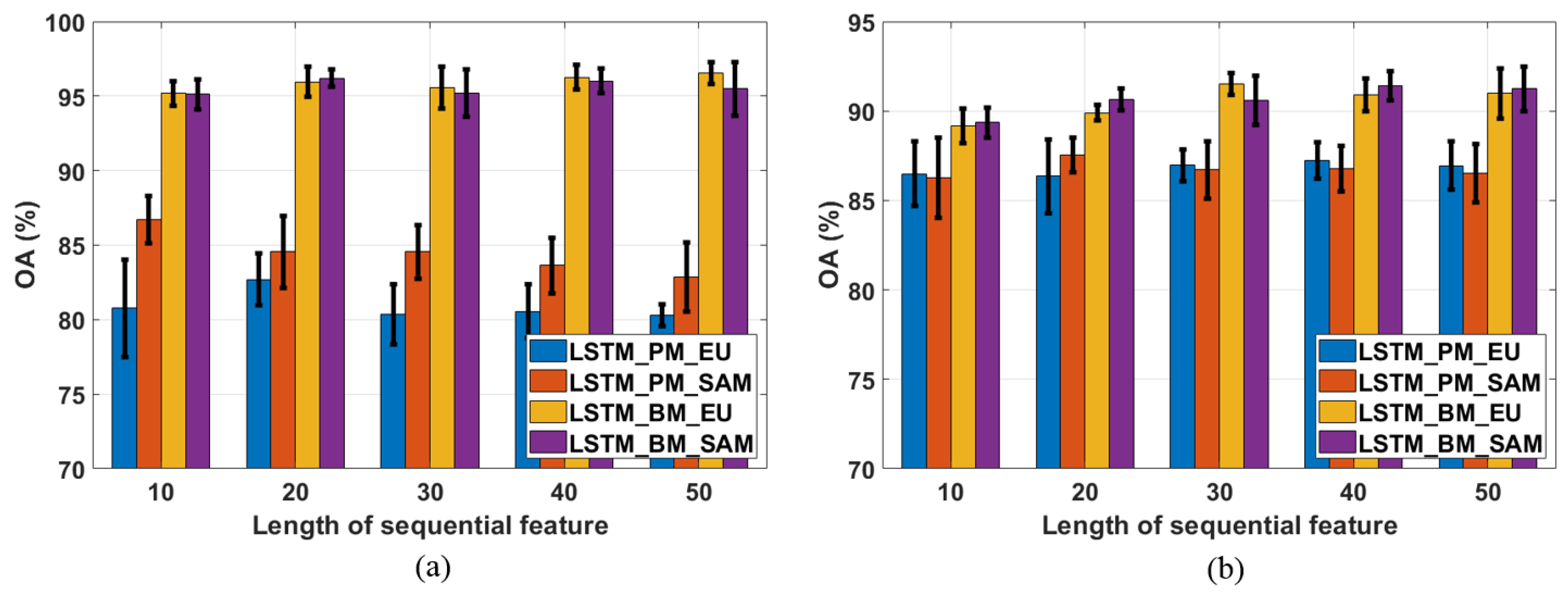
For the first parameter, l, five different lengths (10, 20, 30, 40, and 50) are investigated, while the window size utilized in LSTM_BM_EU and LSTM_BM_SAM is fixed at 5. The results are shown in Figure 6. Regarding the Pavia University data, the best performances for those four proposed methods are obtained with different sequential feature lengths (Figure 6a). Sequential feature lengths of 20 and 10 result in the highest classification OAs for LSTM_PM_EU (82.70%) and LSTM_PM_SAM (86.68%), respectively. For the two block-matching-based methods, the highest OA for LSTM_BM_EU is 96.54% (when l is 50), and setting l to 20 yields the highest-accuracy result for LSTM_BM_SAM. For the pixel-matching-based algorithms, the classification performance of the Euclidean-distance measure is always better than that of SAM. Furthermore, selecting a smaller sequential length (i.e., 10 or 20) is suitable for these two methods. Regarding the block-matching-based methods, Euclidean distance performs better than SAM, except for l is 20. Smaller sequential lengths used with SAM result in higher OAs, but such lengths are not suitable when using the Euclidean distance measure. Nevertheless, the difference in the resultant classification accuracies when employing these two distance measurements in the block-matching scheme is smaller than what it is in pixel-matching scheme. Moreover, the standard deviations for those four methods, across the five sequential lengths, are 1.0020, 1.4280, 0.5342, and 0.4805, for LSTM_PM_EU, LSTM_PM_SAM, LSTM_BM_EU, and LSTM_BM_SAM, respectively, which illustrates that, for the Pavia University data, the block-matching scheme is less sensitive than the pixel-matching method to the sequential-length parameter value.

For the Salinas data, the best choices for l vary depending on the algorithm. As shown in Figure 6b, the length of 40 yields highest accuracies in LSTM_PM_EU and LSTM_BM_SAM. LSTM_PM_SAM achieves best OA when utilizing 20 as the sequential length. Length of 30 results in the highest OA in LSTM_BM_EU. Different from what we observed from Figure 6a, within the pixel-matching-based schemes, SAM always performs better than Euclidean distance except l = 20. Additionally, smaller length provides a better performance for LSTM_PM_SAM (l = 20) but not applicable in LSTM_PM_EU. For the blocking-matching schemes, SAM is the more robust distance measurement since it performs better at four lengths (10, 20, 40, 50), and obtains the highest accuracy with l = 40. Euclidean distance only yields better result compared with SAM at the length of 30 and that is the highest OA among all lengths. For the standard deviations of those four methods, they are 0.3658, 0.4739, 0.9334, and 0.8140, respectively, which exhibits that pixel-matching-based methods is less sensitive than block-matching-based ones. However, due to the higher OAs obtained by LSTM_BM_EU and LSTM_BM_SAM, block-matching schemes are still the applicable methods to classify the Salinas data.

Another investigation of parameter l is its influence on the training time of the LSTM model since a larger l will introduce more parameters to be learned in the LSTM model and will result in more processing time. The training times of different approaches are given in

Table 5. Average training time (min) of LSTM models.

LSTM Parameter	Pavia University Image
Sequential Feature Length	LSTM_PM_EU	LSTM_PM_SAM	LSTM_BM_EU	LSTM_BM_SAM
10	30.88	34.01	29.11	32.00
20	51.14	53.25	49.92	53.73
30	83.39	87.43	77.52	81.63
40	112.49	115.03	105.31	110.75
50	145.29	144.98	132.31	142.07
	Salinas Image
Sequential Feature Length	LSTM_PM_EU	LSTM_PM_SAM	LSTM_BM_EU	LSTM_BM_SAM
10	29.08	34.19	28.47	28.00
20	46.27	49.02	44.96	47.64
30	76.94	85.61	75.83	75.41
40	110.57	117.78	101.10	102.07
50	124.06	147.91	128.13	128.90

. Those training times are the average values obtained from the 10 replications. Different methods with the same l have similar training times for both the Pavia University and Salinas images. However, the training time differs when a different l is applied within one LSTM model. As an example, consider the application of the LSTM_BM_SAM to the Pavia University image; the training time is 32.00 min when l is 10. The training time increases along with utilization of larger l, and it reaches 142.07 min, which is more than four times the minimum training time consumption. Fortunately, BM-based methods are less sensitive compared with PM-based methods regarding the selection of different l, which can be obtained from Figure 6. To balance the computation time cost and classification performance, choosing a smaller l (e.g., 10 or 20) is an appropriate strategy for our proposed methods, even though PM-based methods are relatively more sensitive with respect to parameter l.

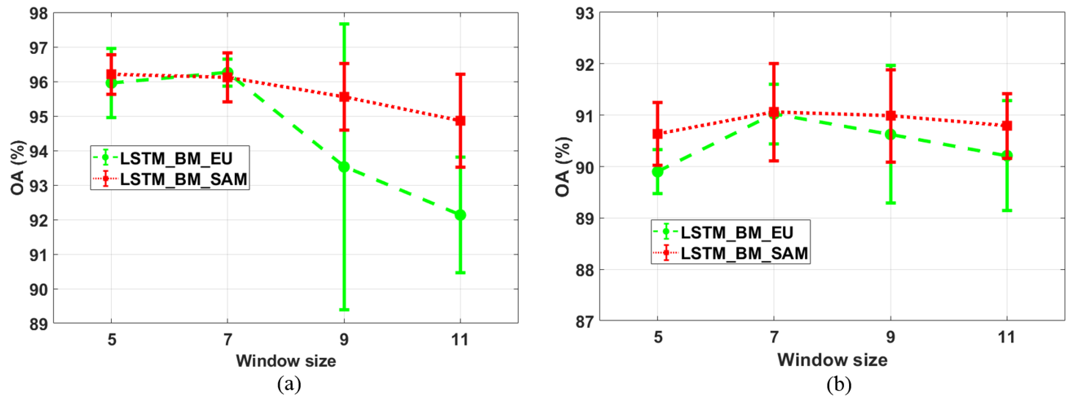
For the second parameter, w, four different window sizes $(5\times 5,7\times 7,9\times 9,11\times 11)$ and two methods (LSTM_BM_EU and LSTM_BM_SAM) are chosen for the comparison experiments, where l is fixed at 20. These results are shown in Figure 7. For the Pavia University data-based results (Figure 7a), the overall classification accuracy of LSTM_BM_SAM is higher than that of LSTM_BM_EU. LSTM_BM_EU obtains a higher OA only when w is set at 7, and that is also the best accuracy across all four window sizes. LSTM_BM_SAM achieves the best performance with a window size of 5 (the smallest window size considered), and the OA decreases as the window size increases. Regarding the Salinas data-based results, given in Figure 7b, the classification accuracies for LSTM_BM_SAM are still higher than those for LSTM_BM_EU, and both of those two methods realize the most accurate results with a window size of 5. Compared with parameter l, the optimal value for w is easier to determine in order to achieve a more accurate classification result. It is predictable that incorporating local spatial contextual information is likely to help better measure the similarity between two pixels, yielding improved classification performance. However, with increasing window size, too many neighboring pixels are included in the calculation, resulting in over-smoothed classification maps, and class spatial boundaries are not preserved. As a consequence, selection of a relatively small window size should introduce sufficient—though not too much—spatial information, leading to higher classification accuracies.

5. Conclusions

In this paper, we propose a novel LSTM HSI classification framework, where unlabeled data are well-exploited in order to construct sequential features from a single HSI. Instead of using spectral features as the sequential data structure of LSTM, similar pixels collected from the entire image are used to construct the respective sequential features. Specifically, when constructing a sequential feature, the similarity between a target pixel and all other pixels in the image is considered. To better depict the similarity between two pixels, two similarity-measuring strategies—pixel-matching and block-matching—are adopted here, where individual spectral features are utilized in the pixel-matching-based schemes, and both spatial and spectral information are employed in block-matching-based schemes. Such schemes take full advantage of unlabeled data in the HSI, as labeled data are almost always limited in nature and difficult to acquire for HSI classification. Moreover, block-matching-based schemes also consider spatial contextual information in the classification process, and it is demonstrated in this research that such schemes are effective in increasing HSI classification. Our proposed methods produce markedly more accurate results when operating on two well-known, extensively-studied HSI datasets compared with other selected baseline algorithms. Particularly regarding the Pavia University image, the LSTM_BM_SAM achieves the best classification performance, with 96.20% OA, which is 11.75% higher than the best result obtained by the three benchmark algorithms, which in this case was 1DCNN, with 84.45% OA. Furthermore, that OA is also higher than those from other three proposed methods (LSTM_PM_EU, LSTM_PM_SAM, and LSTM_BM_EU), with an OA increase of 13.50%, 11.64%, and 0.24%, relative to those respective methods. Additionally, in these experiments, BM-based methods always yield better results compared with their corresponding PM-based methods, which demonstrates the effectiveness and capability of the utilization of spatial contextual information.

Regarding the proposed block-matching method, fixed window sizes are applied for classification. In the future, we will explore adaptive window-size applications, intended to eliminate the phenomenon of over-smoothing in the classified images and to preserve the respective boundaries between different classes. In addition, measuring pixel-wise similarity from the entire HSI more efficiently still needs to be investigated in future research.

The proposed methods in this study combine similarity measurements and recurrent neural networks, and, although in the present study we focus on encoding spatial contextual information, future work may involve implementing these methods in a temporal context (i.e., in a true multi-temporal remote-sensing context).

References

- Haboudane, D.; Miller, J.R.; Pattey, E.; Zarco-Tejada, P.J.; Strachan, I.B. Hyperspectral vegetation indices and novel algorithms for predicting green LAI of crop canopies: Modeling and validation in the context of precision agriculture. Remote Sens. Environ. 2004, 90, 337–352. [Google Scholar] [CrossRef]
- Camps-Valls, G.; Tuia, D.; Bruzzone, L.; Benediktsson, J.A. Advances in hyperspectral image classification: Earth monitoring with statistical learning methods. IEEE Signal Process. Mag. 2014, 31, 45–54. [Google Scholar] [CrossRef]
- Bioucas-Dias, J.M.; Plaza, A.; Camps-Valls, G.; Scheunders, P.; Nasrabadi, N.; Chanussot, J. Hyperspectral remote sensing data analysis and future challenges. IEEE Geosci. Remote Sens. Mag. 2013, 1, 6–36. [Google Scholar] [CrossRef]
- Eismann, M.T.; Meola, J.; Hardie, R.C. Hyperspectral change detection in the presenceof diurnal and seasonal variations. IEEE Trans. Geosci. Remote Sens. 2008, 46, 237–249. [Google Scholar] [CrossRef]
- Wang, Q.; Yuan, Z.; Du, Q.; Li, X. GETNET: A General End-to-End 2-D CNN Framework for Hyperspectral Image Change Detection. IEEE Trans. Geosci. Remote Sens. 2018, 57, 1–11. [Google Scholar] [CrossRef]
- Plaza, A.; Du, Q.; Chang, Y.L.; King, R.L. High performance computing for hyperspectral remote sensing. IEEE J. Sel. Top. Appl. Earth Obs. Remote Sens. 2011, 4, 528–544. [Google Scholar] [CrossRef]
- Ma, L.; Crawford, M.M.; Tian, J. Local manifold learning-based k-nearest-neighbor for hyperspectral image classification. IEEE Trans. Geosci. Remote Sens. 2010, 48, 4099–4109. [Google Scholar] [CrossRef]
- Jia, X.; Richards, J.A. Fast k-NN classification using the cluster-space approach. IEEE Geosci. Remote Sens. Lett. 2005, 2, 225–228. [Google Scholar] [CrossRef]
- Wang, Q.; Zhang, F.; Li, X. Optimal Clustering Framework for Hyperspectral Band Selection. IEEE Trans. Geosci. Remote Sens. 2018, 56, 1–13. [Google Scholar] [CrossRef]
- Melgani, F.; Bruzzone, L. Classification of hyperspectral remote sensing images with support vector machines. IEEE Trans. Geosci. Remote Sens. 2004, 42, 1778–1790. [Google Scholar] [CrossRef] [Green Version]
- Gualtieri, J.; Chettri, S. Support vector machines for classification of hyperspectral data. In Proceedings of the IEEE 2000 International Geoscience and Remote Sensing Symposium (IGARSS 2000), Honolulu, HI, USA, 24–28 July 2000; Volume 2, pp. 813–815. [Google Scholar]
- Tarabalka, Y.; Fauvel, M.; Chanussot, J.; Benediktsson, J.A. SVM and MRF-based method for accurate classification of hyperspectral images. IEEE Geosci. Remote Sens. Lett. 2010, 7, 736–740. [Google Scholar] [CrossRef]
- Chen, Y.; Nasrabadi, N.M.; Tran, T.D. Hyperspectral image classification using dictionary-based sparse representation. IEEE Trans. Geosci. Remote Sens. 2011, 49, 3973–3985. [Google Scholar] [CrossRef]
- Chen, Y.; Nasrabadi, N.M.; Tran, T.D. Hyperspectral image classification via kernel sparse representation. IEEE Trans. Geosci. Remote Sens. 2013, 51, 217–231. [Google Scholar] [CrossRef]
- Zhang, H.; Li, J.; Huang, Y.; Zhang, L. A nonlocal weighted joint sparse representation classification method for hyperspectral imagery. IEEE J. Sel. Top. Appl. Earth Obs. Remote Sens. 2014, 7, 2056–2065. [Google Scholar] [CrossRef]
- Wang, Q.; He, X.; Li, X. Locality and Structure Regularized Low Rank Representation for Hyperspectral Image Classification. IEEE Trans. Geosci. Remote Sens. 2018, 1–13. [Google Scholar] [CrossRef]
- Benediktsson, J.A.; Swain, P.H.; Ersoy, O.K. Conjugate-gradient neural networks in classification of multisource and very-high-dimensional remote sensing data. Int. J. Remote Sens. 1993, 14, 2883–2903. [Google Scholar] [CrossRef]
- Yang, H. A back-propagation neural network for mineralogical mapping from AVIRIS data. Int. J. Remote Sens. 1999, 20, 97–110. [Google Scholar] [CrossRef]
- Gómez-Chova, L.; Camps-Valls, G.; Munoz-Mari, J.; Calpe, J. Semisupervised image classification with Laplacian support vector machines. IEEE Geosci. Remote Sens. Lett. 2008, 5, 336–340. [Google Scholar] [CrossRef]
- Bruzzone, L.; Chi, M.; Marconcini, M. A novel transductive SVM for semisupervised classification of remote-sensing images. IEEE Trans. Geosci. Remote Sens. 2006, 44, 3363–3373. [Google Scholar] [CrossRef]
- Ma, L.; Crawford, M.M.; Yang, X.; Guo, Y. Local-manifold-learning-based graph construction for semisupervised hyperspectral image classification. IEEE Trans. Geosci. Remote Sens. 2015, 53, 2832–2844. [Google Scholar] [CrossRef]
- Ma, L.; Ma, A.; Ju, C.; Li, X. Graph-based semi-supervised learning for spectral-spatial hyperspectral image classification. Pattern Recognit. Lett. 2016, 83, 133–142. [Google Scholar] [CrossRef]
- Wang, Z.; Nasrabadi, N.M.; Huang, T.S. Semisupervised hyperspectral classification using task-driven dictionary learning with Laplacian regularization. IEEE Trans. Geosci. Remote Sens. 2015, 53, 1161–1173. [Google Scholar] [CrossRef]
- Kotsia, I.; Guo, W.; Patras, I. Higher rank support tensor machines for visual recognition. Pattern Recognit. 2012, 45, 4192–4203. [Google Scholar] [CrossRef]
- Zhou, H.; Li, L.; Zhu, H. Tensor regression with applications in neuroimaging data analysis. J. Am. Stat. Assoc. 2013, 108, 540–552. [Google Scholar] [CrossRef]
- Makantasis, K.; Doulamis, A.D.; Doulamis, N.D.; Nikitakis, A. Tensor-based classification models for hyperspectral data analysis. IEEE Trans. Geosci. Remote Sens. 2018, 56, 6884–6898. [Google Scholar] [CrossRef]
- Benediktsson, J.A.; Palmason, J.A.; Sveinsson, J.R. Classification of hyperspectral data from urban areas based on extended morphological profiles. IEEE Trans. Geosci. Remote Sens. 2005, 43, 480–491. [Google Scholar] [CrossRef]
- Zhang, L.; Zhang, L.; Tao, D.; Huang, X. On combining multiple features for hyperspectral remote sensing image classification. IEEE Trans. Geosci. Remote Sens. 2012, 50, 879–893. [Google Scholar] [CrossRef]
- Shi, M.; Healey, G. Using multiband correlation models for the invariant recognition of 3-D hyperspectral textures. IEEE Trans. Geosci. Remote Sens. 2005, 43, 1201–1209. [Google Scholar]
- Zhang, L.; Zhang, L.; Du, B. Deep learning for remote sensing data: A technical tutorial on the state of the art. IEEE Geosci. Remote Sens. Mag. 2016, 4, 22–40. [Google Scholar] [CrossRef]
- Wang, Q.; Liu, S.; Chanussot, J.; Li, X. Scene classification with recurrent attention of VHR remote sensing images. IEEE Trans. Geosci. Remote Sens. 2018, 1–13. [Google Scholar] [CrossRef]
- Chen, Y.; Lin, Z.; Zhao, X.; Wang, G.; Gu, Y. Deep learning-based classification of hyperspectral data. IEEE J. Sel. Top. Appl. Earth Obs. Remote Sens. 2014, 7, 2094–2107. [Google Scholar] [CrossRef]
- Chen, Y.; Zhao, X.; Jia, X. Spectral–spatial classification of hyperspectral data based on deep belief network. IEEE J. Sel. Top. Appl. Earth Obs. Remote Sens. 2015, 8, 2381–2392. [Google Scholar] [CrossRef]
- Girshick, R.; Donahue, J.; Darrell, T.; Malik, J. Rich feature hierarchies for accurate object detection and semantic segmentation. In Proceedings of the IEEE Conference on Computer Vision and Pattern Recognition, Columbus, OH, USA, 23–28 June 2014; pp. 580–587. [Google Scholar]
- Hu, W.; Huang, Y.; Wei, L.; Zhang, F.; Li, H. Deep convolutional neural networks for hyperspectral image classification. J. Sens. 2015, 2015, 1–12. [Google Scholar] [CrossRef]
- Makantasis, K.; Karantzalos, K.; Doulamis, A.; Doulamis, N. Deep supervised learning for hyperspectral data classification through convolutional neural networks. In Proceedings of the IEEE International Geoscience and Remote Sensing Symposium (IGARSS), Milan, Italy, 26–31 July 2015; pp. 4959–4962. [Google Scholar]
- Li, Y.; Zhang, H.; Shen, Q. Spectral–spatial classification of hyperspectral imagery with 3D convolutional neural network. Remote Sens. 2017, 9, 67. [Google Scholar] [CrossRef]
- Elman, J.L. Finding structure in time. Cogn. Sci. 1990, 14, 179–211. [Google Scholar] [CrossRef]
- Mikolov, T.; Karafiát, M.; Burget, L.; Černockỳ, J.; Khudanpur, S. Recurrent neural network based language model. In Proceedings of the Eleventh Annual Conference of the International Speech Communication Association, Chiba, Japan, 26–30 September 2010. [Google Scholar]
- Graves, A.; Mohamed, A.R.; Hinton, G. Speech recognition with deep recurrent neural networks. In Proceedings of the IEEE International Conference on Acoustics, Speech and Signal Processing (ICASSP), Vancouver, BC, Canada, 26–31 May 2013; pp. 6645–6649. [Google Scholar]
- Hochreiter, S.; Schmidhuber, J. Long short-term memory. Neural Comput. 1997, 9, 1735–1780. [Google Scholar] [CrossRef]
- Ienco, D.; Gaetano, R.; Dupaquier, C.; Maurel, P. Land cover classification via multitemporal spatial data by deep recurrent neural networks. IEEE Geosci. Remote Sens. Lett. 2017, 14, 1685–1689. [Google Scholar] [CrossRef]
- Sharma, A.; Liu, X.; Yang, X. Land cover classification from multi-temporal, multi-spectral remotely sensed imagery using patch-based recurrent neural networks. Neural Netw. 2018, 105, 346–355. [Google Scholar] [CrossRef] [Green Version]
- Mou, L.; Ghamisi, P.; Zhu, X.X. Deep recurrent neural networks for hyperspectral image classification. IEEE Trans. Geosci. Remote Sens. 2017, 55, 3639–3655. [Google Scholar] [CrossRef]
- Wu, H.; Prasad, S. Convolutional recurrent neural networks for hyperspectral data classification. Remote Sens. 2017, 9, 298. [Google Scholar] [CrossRef]
- Shi, C.; Pun, C.M. Multi-scale hierarchical recurrent neural networks for hyperspectral image classification. Neurocomputing 2018, 294, 82–93. [Google Scholar] [CrossRef]
- Romera-Paredes, B.; Torr, P.H.S. Recurrent instance segmentation. In Proceedings of the European Conference on Computer Vision, Amsterdam, The Netherlands, 8–16 October 2016; Springer: Berlin/Heidelberg, Germany, 2016; pp. 312–329. [Google Scholar]
- Zhong, Y.; Zhao, J.; Zhang, L. A hybrid object-oriented conditional random field classification framework for high spatial resolution remote sensing imagery. IEEE Trans. Geosci. Remote Sens. 2014, 52, 7023–7037. [Google Scholar] [CrossRef]
- Yin, W.; Kann, K.; Yu, M.; Schütze, H. Comparative study of cnn and rnn for natural language processing. arXiv, 2017; arXiv:1702.01923. [Google Scholar]
- Fan, F.; Deng, Y. Enhancing endmember selection in multiple endmember spectral mixture analysis (MESMA) for urban impervious surface area mapping using spectral angle and spectral distance parameters. Int. J. Appl. Earth Obs. Geoinf. 2014, 33, 290–301. [Google Scholar] [CrossRef]
- Roweis, S.T.; Saul, L.K. Nonlinear dimensionality reduction by locally linear embedding. Science 2000, 290, 2323–2326. [Google Scholar] [CrossRef]
- Belkin, M.; Niyogi, P. Laplacian eigenmaps for dimensionality reduction and data representation. Neural Comput. 2003, 15, 1373–1396. [Google Scholar] [CrossRef]
- Asner, G.P.; Heidebrecht, K.B. Spectral unmixing of vegetation, soil and dry carbon cover in arid regions: Comparing multispectral and hyperspectral observations. Int. J. Remote Sens. 2002, 23, 3939–3958. [Google Scholar] [CrossRef]
- Tobler, W.R. A computer movie simulating urban growth in the Detroit region. Econ. Geogr. 1970, 46, 234–240. [Google Scholar] [CrossRef]
- Pu, H.; Chen, Z.; Wang, B.; Jiang, G.M. A novel spatial–spectral similarity measure for dimensionality reduction and classification of hyperspectral imagery. IEEE Trans. Geosci. Remote Sens. 2014, 52, 7008–7022. [Google Scholar]
- Huttenlocher, D.P.; Klanderman, G.A.; Rucklidge, W.J. Comparing images using the Hausdorff distance. IEEE Trans. Pattern Anal. Mach. Intell. 1993, 15, 850–863. [Google Scholar] [CrossRef]
- Congalton, R.G. A review of assessing the accuracy of classifications of remotely sensed data. Remote Sens. Environ. 1991, 37, 35–46. [Google Scholar] [CrossRef]
Figure 1.
Architecture of the proposed methods.
Figure 2.
The basic structure of an unrolled long short-term memory LSTM unit.
Figure 3.
False-color image composites and their corresponding ground-reference data. (a) false-color composite of Pavia University image bands (R: band 55, G: band 33, and B: band 13); (b) ground-reference data (with class legend) for the Pavia University image; (c) false-color composite of Salinas image bands (R: band 57, G: band 27, and G: band 17); (d) ground-reference data (with class legend) for the Salinas image.
Figure 4.
Classification maps for the Pavia University image from the fifth trial: (a) ground-reference map; (b) SVM, with OA = 80.04%; (c) 1DCNN, with OA = 78.32%; (d) 1DLSTM, with OA = 83.72%; (e) LSTM_PM_EU, with OA = 83.81%; (f) LSTM_PM_SAM, with OA = 86.78%; (g) LSTM_BM_EU, with OA = 93.18%; and (h) LSTM_BM_SAM, with OA = 96.01%. The red-rectangle and red-circle annotations represent sample areas of interest, discussed in the text.
Figure 5.
Classification maps of Salinas image from the fifth trial: (a) ground-reference map; (b) SVM, with OA = 83.38%; (c) 1DCNN, with OA = 87.00%; (d) 1DLSTM, with OA = 86.85%; (e) LSTM_PM_EU, with OA = 86.21%; (f) LSTM_PM_SAM, with OA = 87.13%; (g) LSTM_BM_EU, with OA = 90.02%; and (h) LSTM_BM_SAM, with OA = 90.72%. The red-circle and red-rectangle annotations represent sample areas of interest, discussed in the text.
Figure 6.
Analysis of different sequential feature lengths. (a) OAs based on the Pavia University image data; and (b) OAs based on the Salinas image data.
Figure 7.
Analysis of different window sizes. (a) OAs based on the Pavia University image data; and (b) OAs based on the Salinas image data.