Deep Self-Learning Network for Adaptive Pansharpening


School of Geography and Planning, Guangdong Provincial Key Laboratory of Urbanization and Geo-simulation, Center of Integrated Geographic Information Analysis, Sun Yat-sen University (SYSU), Guangzhou 510275, China
*
Author to whom correspondence should be addressed.
Remote Sens. 2019, 11(20), 2395; https://0-doi-org.brum.beds.ac.uk/10.3390/rs11202395
Submission received: 10 September 2019
/
Revised: 12 October 2019
/
Accepted: 13 October 2019
/
Published: 16 October 2019
(This article belongs to the Special Issue Remote Sensing Image Restoration and Reconstruction)
Abstract
:Deep learning (DL)-based paradigms have recently made many advances in image pansharpening. However, most of the existing methods directly downscale the multispectral (MSI) and panchromatic (PAN) images with default blur kernel to construct the training set, which will lead to the deteriorative results when the real image does not obey this degradation. In this paper, a deep self-learning (DSL) network is proposed for adaptive image pansharpening. First, rather than using the fixed blur kernel, a point spread function (PSF) estimation algorithm is proposed to obtain the blur kernel of the MSI. Second, an edge-detection-based pixel-to-pixel image registration method is designed to recover the local misalignments between MSI and PAN. Third, the original data is downscaled by the estimated PSF and the pansharpening network is trained in the down-sampled domain. The high-resolution result can be finally predicted by the trained DSL network using the original MSI and PAN. Extensive experiments on three images collected by different satellites prove the superiority of our DSL technique, compared with some state-of-the-art approaches.
1. Introduction
The past few years have witnessed the dramatic leap in the remotely sensed imaging. Nonetheless, it is sometimes difficult to obtain the high-resolution satellite images due to the hardware limitations [1]. Pansharpening is a technique of merging the high-resolution panchromatic (PAN) and low-resolution multispectral images (MSI) to synthesize a new high-resolution multispectral (HRMSI) image. With desirable resolution, the created image can yield better interpretation capabilities in applications such as land-use classification [2,3], target recognition [4], detailed land monitoring [5], and change detection [6].
A number of pansharpening methods have been proposed and can be generally divided into four classes: Component substitution (CS), multiresolution analysis (MRA), hybrid algorithms, and learning-based methods. The CS method contains Principle component analysis (PCA) [7], Intensity-hue-saturation transform (IHS) [8], Gram–Schmidt transform (GS) [9], Brovey transform [10], etc. Those algorithms are efficient in terms of the execution time and are able to render the spatial details of PAN with high fidelity. However, this class may lead to the serious spectral distortion. The MRA approach includes Decimated wavelet transform (DWT) [11], “-trous” wavelet transform (ATWT) [12], Laplacian pyramid [13], Contourlets [14], etc. This category is good at preserving the spectral information, while the fusion result suffers from the spatial misalignments. The hybrid method combines the advantages of the above two classes and, therefore, the fusion results can balance the trade-off between the spatial and spectral information. This class contains the methods such as Guided filter in PCA domain (GF-PCA) [15] and Non-separable wavelet frame transform (NWFT) [16]. The learning-based model aims at searching for the relationships between MSI, PAN, and the corresponding HRMSI. Since pansharpening is an ill-posed problem, the selection of prior constraints is critical to make the reliable solution [17,18]. As such, the pansharpening can be intrinsically viewed as an optimization problem. The representative methods of this category include the Matrix factorization [19], the Dictionary learning [20], the Bayesian model [21], etc. However, the performances of those methods depend heavily on the prior assumptions and the learning abilities, which can be the difficulties in application. Recently, deep learning (DL) has shown much potential in various image-processing applications such as scene classification [22], super-resolution [23,24], and face recognition [25], and has become a thriving area in the image pansharpening in the last four years.
The basic idea of DL-based methods is to find the image priors via an end-to-end mapping from the training samples of MSI, PAN, and HRMSI, by means of several convolutional and activation layers [26]. The earliest work of the DL-based pansharpening can be traced back to the Sparse auto-encoder (SAE) method by [27]. In [28,29], to resolve the super-resolution (SR) problem, the authors propose the SRCNN model and open the door for the convolutional neural networks (CNN)-based image restoration. After that, CNN has been extensively adopted for the image fusion tasks. For instance, [30] uses the SRCNN to process the nonlinear pansharpening, demonstrating the superiority of CNN method as comparing with the traditional algorithms. The variant structures such as residual network [31,32], very deep CNN [33], and generative adversarial model [34] are also designed to solve the pansharpening problem. To simultaneously obtain the spatial enhancement and the spectral preservation, [35] proposes a 3D-CNN framework for image fusion and [36] designs a two-branches pansharpening network, where the spatial and spectral information is separately processed. Apart from the developments on the network architecture, some methods take advantage of the other characteristics of the image to improve the fusion performance. In [30], some radiometric indices from MSI are extracted as the input. In [37], the authors train the model with high-pass elements of PAN to reduce the training burden and mitigate the quantitative deviation between the different satellites. In [38], image patches are clustered according to the geometric attributes and processed via multiple fusion networks, which significantly improves the pansharpening accuracy. Combining the DL methods with traditional pansharpening algorithms is also a research topic. For instance, [39] combines the CNN with MRA framework and, in [40], DL with GS approach are adopted. To sum up, DL is a powerful tool for image pansharpening and achieves the state-of-the-art [41]. The main advantages of DL model mainly manifest in three aspects. First, it can adaptively extract the effective features to obtain the best performance, instead of using the handcrafted design. Second, it can automatically model the nonlinear relationship from the training set, rather than relying on the complex prior assumptions. Third, it focuses on the local similarities between the input and the target, thus, the reconstruction result is able to preserve the spatial details.
However, regardless of the superiority of the DL-based pansharpening, some problems, which are not discussed in the abovementioned DL methods, can still be the obstacles in reality. First, due to the unavailability of external high-resolution examples, DL methods tend to construct the sufficient training samples by downscaling the MSI and PAN themselves. However, most of the existing data-generated methods simply adopt the default blur (i.e., fixed Gaussian kernel) rather than obeying the true point spread function (PSF) in the MSI. Training on the samples derived from the wrong blur kernel will lead to the serious deterioration for the pansharpening results [42]. Some methods adopt the PSF directly from the parameters of the satellites, which is not feasible for different or even unknown sources [43]. Second, DL-based image pansharpening is sensitive to local shifts, and the inaccurate overlap between the original MSI and PAN may exert the devastating effects on the fusion results. Nevertheless, traditional coregistration methods rely on the orthorectification provided by the digital surface model and accurate ground control-point selection [44], which requires the expensive manual work.
In order to solve the abovementioned problems and improve the adaptability of the DL methods, in this paper, we have proposed a deep self-learning (DSL) model for pansharpening. The DSL algorithm can be divided into three steps. First, to adaptively estimate the PSF of the MSI, which is used to degrade its higher-resolution counterpart, we propose a learning-based PSF estimation technique to predict the true blur kernel in MSI. We design a deep neural network named CNN-1 to obtain the relationship between the MSI and its PSF. Second, we develop an image alignment method to obtain the correct overlap pixel-to-pixel, where the spatial attributes for the registration metrics are extracted by the edge detection. It is an unsupervised technique which does not require any manual labor. Finally, we construct a simple and flexible network named CNN-2 to learn the prior relationship between the training samples, and establish the training set by downscaling the original MSI and PAN with the estimated PSF and train the CNN-2 in the down-sampled domain. Based on the trained CNN-2, we can obtain the pansharpening result using MSI and PAN. Compared with the existing literature, the contributions of this paper are threefold:
- We propose a CNN-1 for the PSF calculation, which can directly estimate the blur kernel of the MSI without its higher-resolution counterpart.
- We develop an edge-detection-based algorithm for unsupervised image registration with the pixel shifts. The method ensures the same overlaps between the MSI and PAN at the pixel level.
- We construct the training set using the estimated PSF and present a CNN-2 to learn the end-to-end pansharpening. This enables the model to adaptively learn the mapping for any dataset.
The remainder of this paper is organized as follows. Section 2 introduces the proposed DSL framework, where the PSF estimation, the image registration, and the image fusion are described in detail. Section 3 reports the experimental results and the corresponding analyses on the three remote sensing images. Section 4 gives some discussions about the essential parameters and the conclusion is drawn in Section 5.
2. Proposed Method
2.1. General Architecture
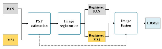
In this section, we introduce the DSL framework in detail. The block diagram of our method is displayed in Figure 1, which consists of three parts. First, we design a CNN-1 to learn the relationship between the blurred image and its corresponding kernel, where the training samples are generated from PAN. After the training stage, the PSF of MSI can be directly estimated using the trained CNN-1 and we adopt the to combine the prediction results. Due to the lack of clearer counterpart of MSI, the estimation can be viewed as an unsupervised manner. The output of this block is the predicted PSF of MSI. Second, we develop an unsupervised registration method to recover the local misalignments between MSI and PAN. The PAN is shifted with several pixels and, to obtain the same spatial size as MSI, it is downscaled with the estimated PSF. Then, the edges of MSI and PAN are detected and we compute the distance between the edge maps. The shift that minimizes the distance is adopted to register the images and we output the registered MSI and PAN in this block. Third, we establish a CNN-2 to implement the nonlinear mapping for the image pansharpening. The training samples are generated by downscaling the registered MSI and PAN with the estimated PSF. The HRMSI can be finally predicted from the trained CNN-2, using the registered MSI and PAN.
2.2. PSF Estimation
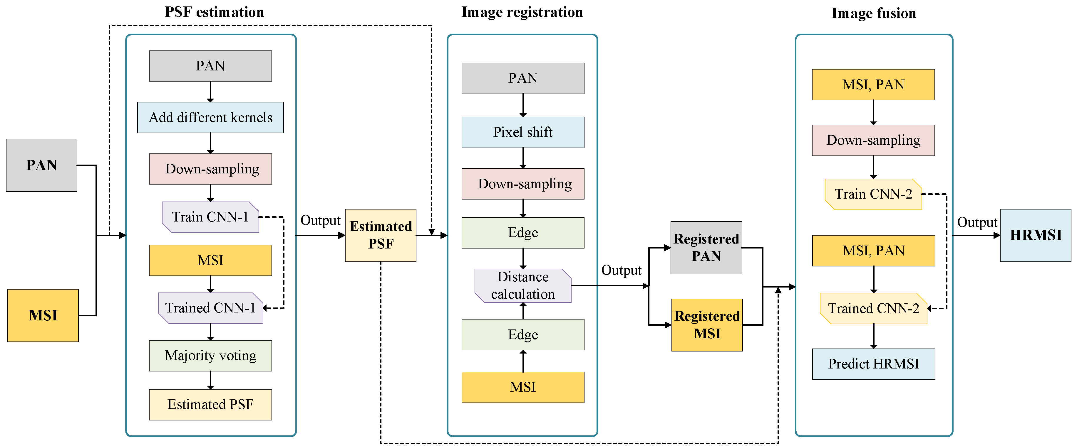
The PSF denotes the response of the sensor to a point source, and it is also noticed as the blur kernel. Here, we propose a new estimation method to predict the PSF of MSI via the CNN-1 model, where the architecture of the CNN-1 is displayed in Figure 2. It consists of five convolutional layers [45], and for each layer it has 64 kernels of size . After each convolutional layer, we set the Rectified linear unit (ReLU) activation [46]. At the end of the last convolutional layer, the activation is set as the Softmax [47], which can output the posterior probability distributions for each of the results. The max-pooling layer [45], dropout layer [46], and the dense layer are designed to reduce the parameters and boost the training.
When it is possible to use the CNN-1 to predict the internal PSF for the MSI data, a fundamental assumption is that there exists a one-to-one relationship between the down-sampled image and its corresponding blur kernel. In order to explore this relationship, we should analyze the formation of the PSF and the degrade function. It is known that for the satellite images, the main type of the PSF is the Gaussian blur [48], which can be formulated as
where denotes the size of the blur regions along the spatial domain and denotes the standard deviation of the Gaussian distribution to be estimated. Usually, is set according to and therefore, can be regarded as relying on the only parameter .
For convenience, we denote the PAN as , and its down-sampled version can be denoted as , which can be defined using the following equation:
where k and denote the blur kernel and the down-sampling operation, respectively. In our analysis, the addictive noise is not considered and we assume a noise-free condition. Since the down-sampler is fixed with the regular sampling, the degrade function can be only defined by k. According to the above analysis, k is decided by its . Therefore, for the certain , can be formulated as follows:
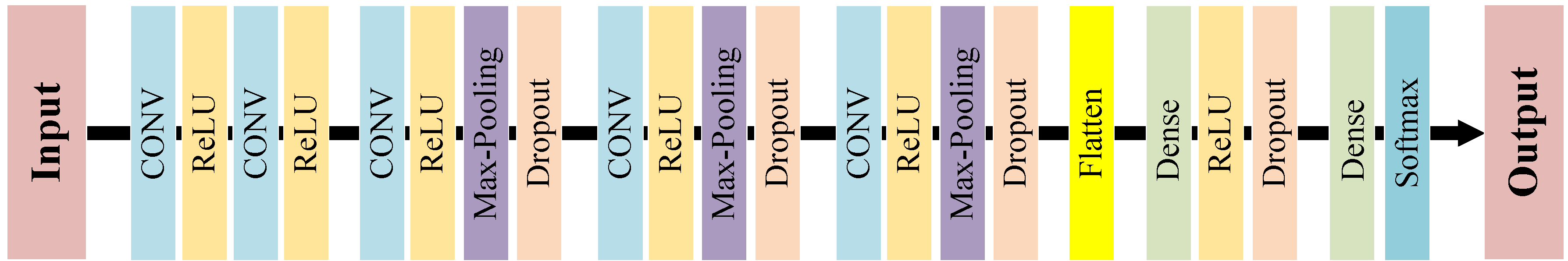
From the above equation, it is possible to construct the dependent relationships between the down-sampled result and its corresponding blur kernel. This phenomenon can be visually observed in Figure 3 that, when is fixed, the blurred result changes according to the adopted . We use the designed CNN-1 to learn this relationship, where the CNN-1 is trained with the and the predefined .
First, we use the predefined vector to downscale the and generate a different degraded version . Then, we construct the pair of samples to train the CNN-1. The input of the network is the downscaled , while the target of the output is . After the training, the end-to-end relationship between the down-sampled images and their corresponding blur kernels is learned. Sequentially, for a new MSI example (we denote it as ), it is intuitively able to predict its internal blur kernel through the trained CNN-1. Specifically, we extract each band of MSI to the trained network, then we summarize the results of each band to make the final prediction.
In order to construct the training and testing samples for the CNN-1, the and are sliced to the patches with 33 × 33 pixels. To train the CNN-1 model, we adopt the cross-entropy as the cost function.
After the training, we estimate the kernel for each of the testing patches and use the to combine the results. The , which emerges most frequently, is determined to be the final prediction, thus the estimation of PSF in is implemented. The output using the can be written as
where j denotes the number of image patches and stands for counting the frequencies of the output . The CNN-1-based kernel estimation is summarized in Algorithm 1.
| Algorithm 1 The CNN-1-based blur estimation procedure of the proposed method. |
| Require: |
| - : PAN; |
| - : MSI; |
| - : A vector of predefined parameters of the blur kernel; |
| - The designed CNN-1. |
| Blur Estimation: |
| - Slice to the patches of the size : . |
| - Use to generate the various down-sampled version of . |
| - Train the CNN-1 via and . |
| - Slice each of the band of to the patches of the size . |
| - Use the trained CNN-1 to predict the for . |
| - Use the to combine the results of and output the final prediction . |
| Ensure: |
| - : The estimated blur kernel in . |
2.3. Edge-Detection-Based Image Registration
For convenience, the MSI and PAN are denoted as and , respectively. Assume that the is of the size and, in an ideal condition, the is of the size , where t denotes the spatial scale between the and . However, the size of can always be in reality, where and denote the pixel redundances. Therefore, there exists the local misalignments. To recover those misalignments and ensure the same overlap between the and at the pixel level, we propose an edge-based image registration algorithm. The downscaled of using the estimated blur kernel can be written as
When and are correctly registered, the pixel alignment of the land-covers of the is supposed to be the same as . Thus, it is a feasible way to explore the local rectification using the pixel-to-pixel matching. However, the deviation of the sources makes it difficult to directly compare the reflectance over the two data. To solve this problem, the edge is exploited to calculate the spatial characteristics for the and . It is a flexible tool to estimate the high-pass elements of each land-cover. For convenience, we use the Canny algorithm [49] to detect the edge, which can be directly obtained by function from Matlab.
The procedure of the edge-detection-based image registration method can be specifically described as following steps. First, we use the original coarse centroid of the and to initialize the registration. The coarse centroid for is set as and, for , it is . The two centroids may not represent the exact same location, and the images should be rectified via pixel shifts. Thus, we shift the with pixels horizontally, vertically, and the combination of them, respectively, before the downscaling. It is noteworthy that the shift can not be processed in the down-sampled domain, because the local misregistration will be diminished with the decimation. We denote the shifted image as . Second, we downscale the to the and calculate the edges of it, as well as the edges of each band of . The edges of and can be noticed as and . We calculate the edges in the down-sampled domain instead of enlarging the to the size of , because it is difficult to detect the edges of the low-resolution interpolated . Finally, we can compute the distance between the and as follows:
We pick out the and the corresponding directions which minimize the . Then, the local registration between and is implemented with pixel shifts. The proposed image registration is summarized in Algorithm 2.
| Algorithm 2 The edge-detection-based image registration procedure of the proposed method. |
| Require: |
| -: MSI; |
| -: PAN; |
| -: Estimated PSF of MSI. |
| Edge-Detection-based Registration: |
| - Shift the toward horizontal and vertical directions and the combination of them with pixels to , respectively. |
| - Downscale the to using . |
| - Calculate the edges and of the and each band of using Canny algorithm. |
| - Calculate the distance between and pixel-to-pixel. |
| - Select the directions and the corresponding which minimizes . |
| - Apply the and its directions on and output the registered images. |
| Ensure: |
| - The registered and . |
2.4. Adaptive Pansharpening
In this section, we introduce an adaptive pansharpening model to implement the MSI and PAN image fusion using the estimated PSF. Several schemes have been proposed to make use of the PSF to achieve the high-quality image restoration result. In [50], the authors exploit the hybrid color mapping (HCM) algorithm for the hyperspectral and color image fusion, where the hyperspectral images are deblurred and super-resolved with the Plug-and-play ADMM method [51]. Also, ref. [52] introduces a hyper-Laplacian prior-based image deblurring and super-resolution method using PSF. In this paper, we directly adopt a deep learning model to learn the relationships between the degraded MSI and PAN and the high-resolution MSI with the estimated PSF.
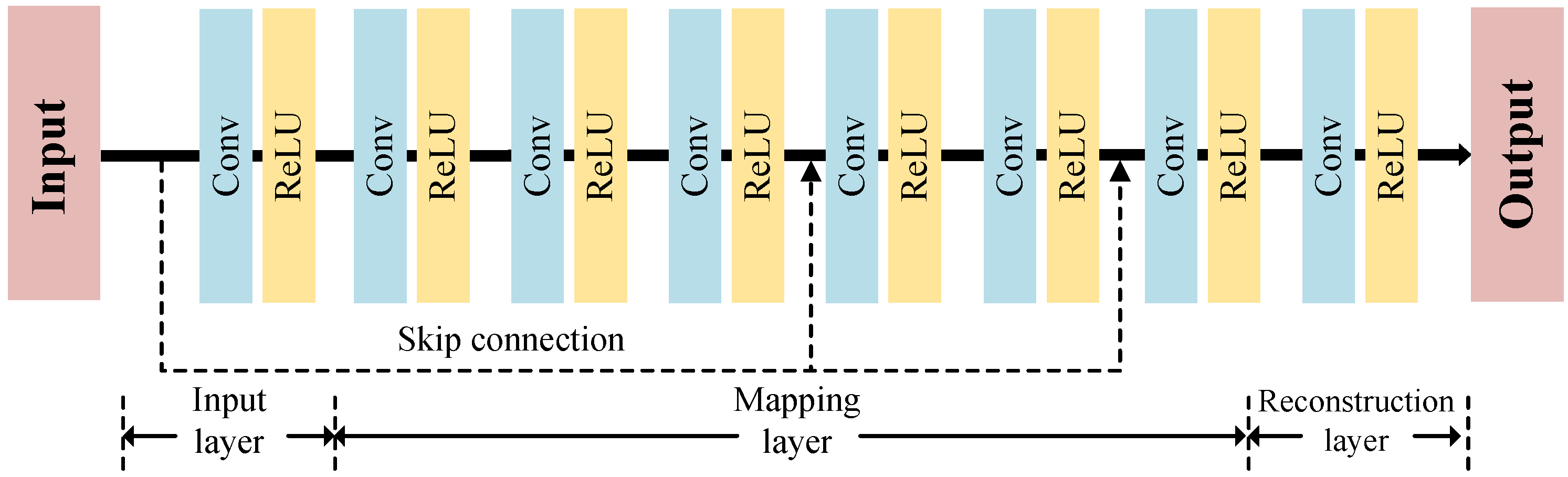
To learn the nonlinear mapping for the MSI and PAN pansharpening, we propose a CNN-2 with the structure in Figure 4. It is a simple and flexible network, which consists of the input layer, the nonlinear mapping layer, and the reconstruction layer, and they can be defined as
where f denotes the extracted features by the convolutional kernels of the corresponding layer, means the weights and bias, and is the ReLU activation for the filter responses of each layer. ⊗ denotes the convolutional operation. To propagate the input information and alleviate the gradient vanishment problem, we adopt two skip connections. In addition, after each convolutional operation, we adopt the zero padding to get the same size with the inputs.
To establish an adaptive pansharpening model for any given data, we train the CNN-2 using the downscaled samples on the lower-resolution domain and apply the model on the MSI and PAN themselves. This operation requires the base assumption: With the same degradation, the mapping relationship between the low- and high-resolution version of the image is scale-invariant. Therefore, it is feasible to use the low-resolution trained model for the high-resolution pansharpening. First, we down-sample the registered and from Section 2.3 to the and , respectively, via the PSF, which is estimated from Section 2.2:
It is noteworthy that by synthetically down-sampling the and using the above equation, unlimited training samples can be virtually generated. Then, we adopt the as well as to train the pansharpening CNN-2, with the target to obtain the high-resolution image that is as similar to the as possible. However, the image size of and is different to input and, to solve this problem, we can up-sample the to the spatial size of with bicubic interpolation. Then, we concatenate the interpolated and as the input of the pansharpening network. The pansharpening with CNN-2 can be formulated as follows:
where denotes the network parameters of the CNN-2. The purpose of the training stage is to obtain the which can correctly represent the relationship among the training samples. In order to train this model, the Mean-square-error (MSE) is adopted as the loss function:
where u denotes the number of input patches. From the equation, the MSE minimizes the average pixelwise error between the generated and the reference samples.
With the training on the samples whose degradation is consistent with the real MSI, the proposed CNN-2 can adaptively learn the mapping according to the given data. When we implemented the end-to-end learning, we input the registered and to the trained CNN-2 and obtain the estimated HRMSI :
The predicted is the corresponding high-resolution pansharpening result for the MSI and PAN, and it is the final output of our DSL model. The proposed adaptive image pansharpening is summarized in Algorithm 3.
| Algorithm 3 The adaptive image pansharpening procedure of the proposed method. |
| Require: |
| - : Registered MSI; |
| - : Registered PAN; |
| - : Estimated PSF of MSI; |
| - The designed CNN-2. |
| Adaptive Pansharpening: |
| - Downscale the , to the and , respectively, using . |
| - Train the pansharpening CNN-2 via and the bicubic-interpolated with the objective , using the MSE loss function. |
| - Input and the interpolated into the trained CNN-2, and obtain the final prediction . |
| Ensure: |
| - : The predicted HRMSI. |
3. Experiments
3.1. Data Description
Three remotely sensed datasets are used in our experiments, including the GF-2, the GF-1, and the JL-1A satellite images. The details of the three images are described as follows.
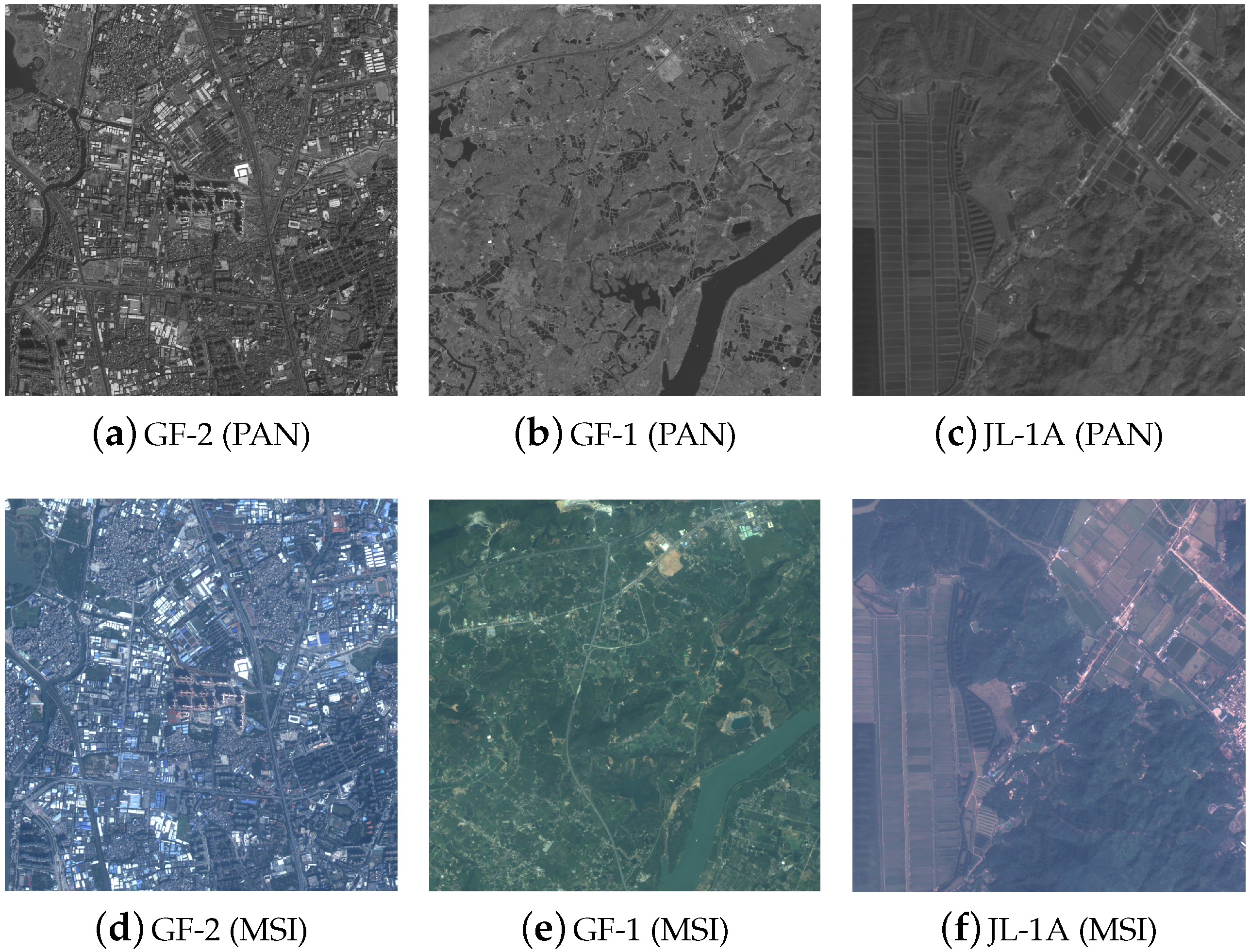
- GF-2 is a high-resolution optical earth observation satellite which is independently developed by China. It has two PAN/MSI cameras, where the spatial resolution is 1 m and 4 m, respectively. The MSI has four spectral channels including the blue, green, red, and near-infrared (NIR) bands. The data we used in this paper reveal the urban area of Guangzhou city, China and were collected on 4 November 2016. Figure 5a,d depict the PAN and MSI of this data, respectively.
- GF-1 is configured with two PAN and MSI with the spatial resolution 2 m and 8 m, respectively, and another four MSI cameras with 16 m resolution. The 8 m MSI includes four spectral bands including the blue, green, red, and the NIR. In this paper, we adopt the 2 m PAN and the 8 m MSI as the experimental data and the research region is the Guangzhou city, China. The data were acquired on 24 October 2015. The PAN and MSI of this data are displayed in Figure 5b,e, respectively.
- JL-1A is independently developed by China and was launched in 2015. The satellite provides a PAN at 0.72 m and a MSI at 2.88 m, respectively. The MSI has three optical bands including blue, green, and red. The data in this paper cover the region of Qi’ao island in Zhuhai City, China and were collected on 3 January 2017. Figure 5c,f show the PAN and MSI of the data, respectively.
3.2. Experimental Setup
In order to validate the performance of the proposed DSL framework, 10 state-of-the-art methods have been used for comparison. The descriptions of the comparison algorithms are displayed in Table 1. Matlab codes are directly downloaded from the website (https://github.com/sjtrny/FuseBox) (http://openremotesensing.net/). The DL based models are reproduced according to the corresponding literatures using Python language.
Two different hardware environments, including CPU and GPU, have been used to conduct the experiments. The CPU environment is composed of an Intel Core i7-6700 @ 3.40 GHz, with 24 GB of DDR4 RAM. The software environment in CPU is Matlab 2017a on a Windows 10 operation system. The GPU environment is composed of the NVIDIA Tesla K80, with 12 GB of RAM. The software environment in GPU is the Python 3.6. The comparison methods, which do not belong to the DL family, are implemented in CPU; and the DL methods are set in the GPU in the Keras (https://keras.io/) framework with Tensorflow (https://www.tensorflow.org/) backend.
For the three satellite data in the experiments, the size of the MSI and PAN are set as and , respectively. However, we can not evaluate the pansharpening results of them since the high-resolution ground-truth is not available in practice. Therefore, we adopt the original multispectral satellite images as the ground-truth and downscale the original multispectral and panchromatic images to the lower-resolution with the predefined “true” to synthesize the MSI and PAN. To simulate different degradations, the “true” is predefined as 1.5, 2, and 4.5, respectively, for the three datasets. For convenience, the blur region is fixed as 21, because it is enough to contain most of the energy for the three kernels.
For the CNN-1-based PSF estimation, a series of blur kernels are predefined to generate the training set. For GF-2 and GF-1, n is set as 8 and is set as . For JL-1A, n is set as 6 and is set as , because this dataset is visually more blurry than the other two images and it is intuitively insensitive to the slight kernel variance. To train the CNN-1, images are sliced to the patches of pixels and 7688 training samples are generated. 20% of the samples are used to validate the network. We use the Stochastic Gradient Descend (SGD) optimizer with the learning rate of 0.01 and the momentum of 0.9. The number of epochs of training is set as 1000.
For the CNN-2 model, the training images are not sliced to the small patches because the size of the images is not large. Therefore, the number of the training sample is only one and the model converges quickly. We use the Adam optimizer with the initial learning rate of 5 × 10, which can be reduced by a factor of 2 if the loss does not decrease within 25 epochs. The epoch number of the training is set as 1000.
To evaluate the properties of the obtained result, six quantitative indexes are used in this paper: Root-mean-square error (RMSE), peak signal noise ratio (PSNR), structure similarity (SSIM), spectral angle mapper (SAM), cross correlation (CC), and (ERGAS) [17]. Additionally, we display the execution time for each method. For the DL-based methods, it denotes the training time. RMSE and PSNR denote the quantitative similarity between the generated and the reference images, while SSIM reveals the structure similarity, CC indicates the correlation, and SAM and ERGAS mean the spectral preservation between two signals. For PSNR, SSIM, and CC, larger value indicates better performance; for RMSE, SAM, and ERGAS, smaller denotes better. The Matlab codes of those metrics are publicly available (http://openremotesensing.net/). All pansharpening results are normalized before quantitative evaluation.
3.3. Experimental Results
3.3.1. Comparison with Pansharpening Methods
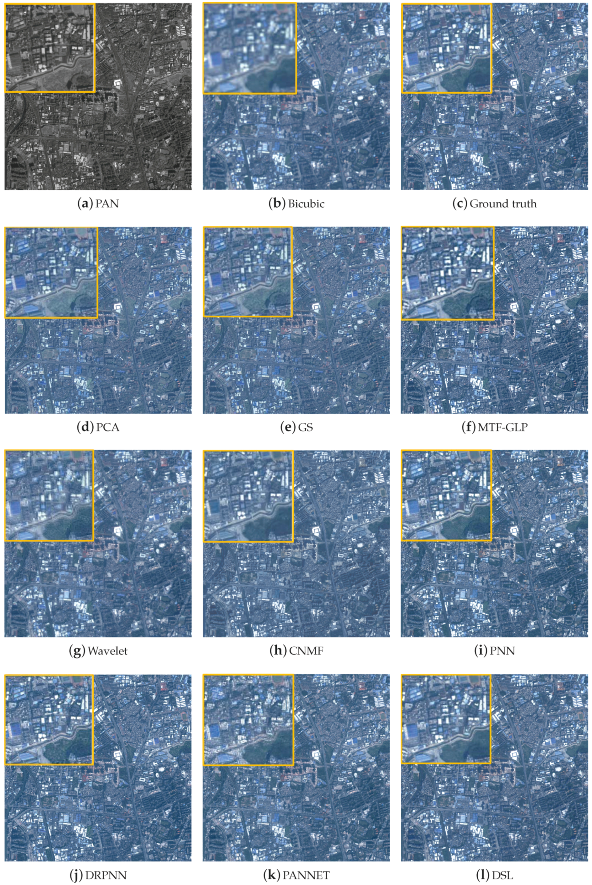
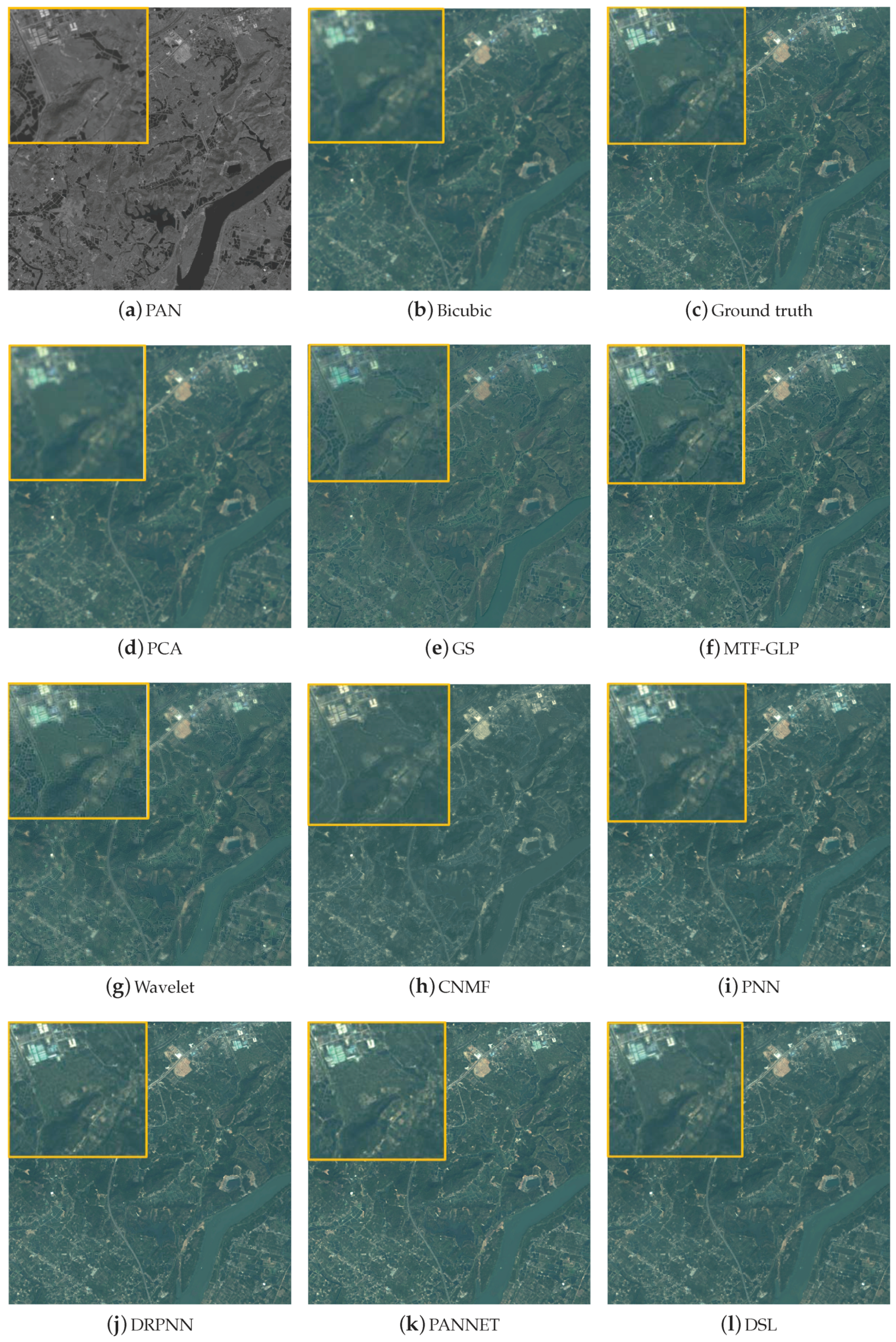
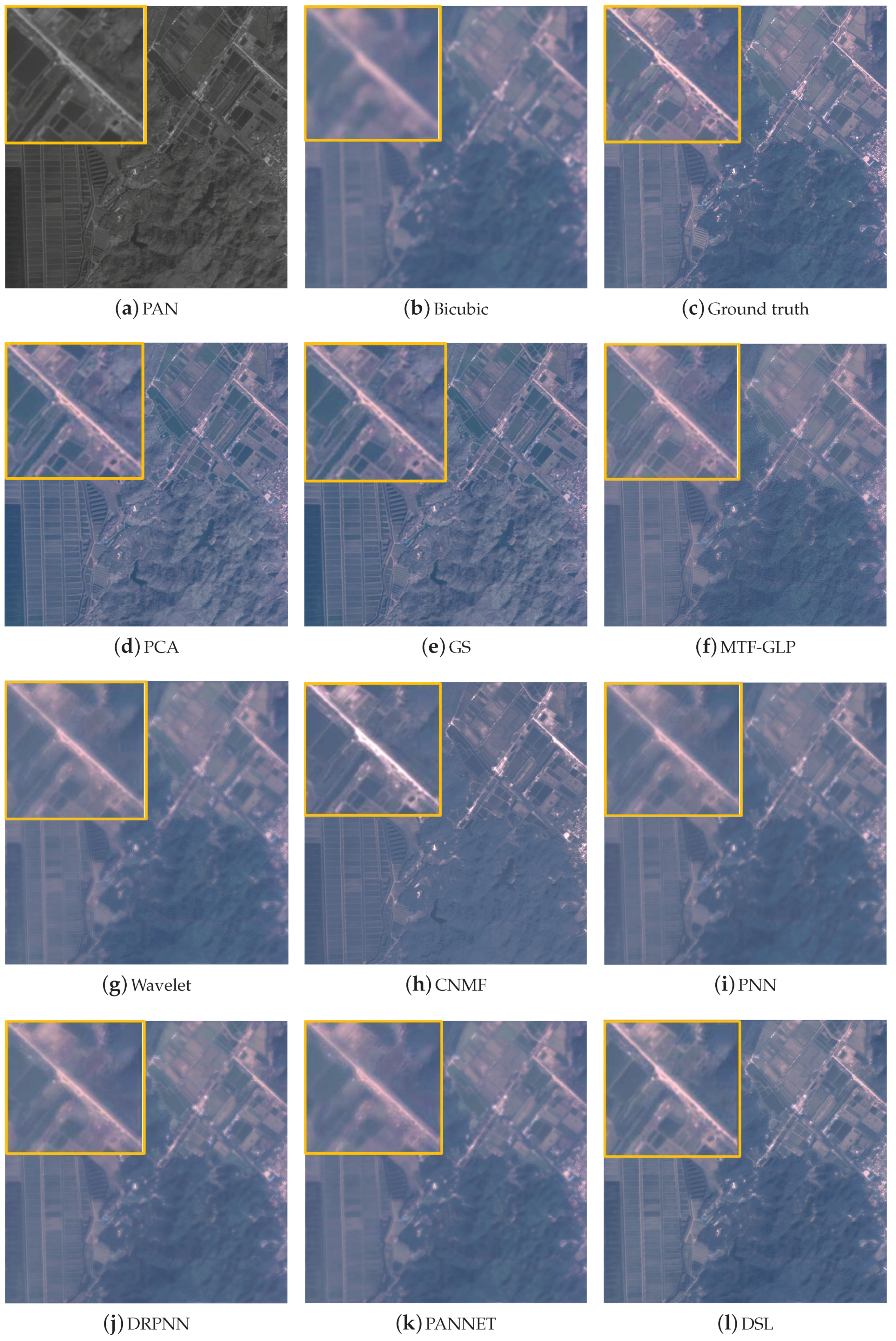
A group of the state-of-the-art methods are compared with the proposed method. For fair comparison, the images for those methods are all locally registered. For the DL-based methods, the training samples are generated using the degradation with the default of 2.5. The quantitative results of different methods for the three datasets are displayed in Table 2, Table 3 and Table 4. Figure 6, Figure 7 and Figure 8 show the visual results of them. Additionally, we display a zoom-in subregion on the top-left corner for better legibility.
From Figure 6, Figure 7 and Figure 8, we can observe that the image quality of all results is significantly higher than the bicubic interpolation, illustrating the effectiveness of the pansharpening procedure. However, among them, the lack of spatial and spectral fidelities can still be observed. First, the methods that do not belong to DL, PCA, GS, and CNMF are caught in serious spectral distortion, while Wavelet is inferior in the spatial domain. For instance, in Figure 6, the color of PCA and CNMF is much darker than the reference. The CNMF tends to be blurry, while Wavelet can lead to some artifacts. Second, for the DL-based methods, PNN, DRPNN, and DSL obtain the reasonable visual results in terms of the spectral preservation. However, the comparison methods get deteriorated results for the spatial reconstruction. For example, unrealistic details can be observed from the PANNET in Figure 6, where the black patches broadly distribute on the architectures. In Figure 6 and Figure 7, PNN and DRPNN also result in many artifacts, while in Figure 8, their results are more blurry as compared with the reference. It is because for those competitors, the blur kernels used for constructing the training samples deviate from the true one, and the wrong kernels significantly damage the fusion performances. If the kernels are larger than the reality (i.e., GF-2 and GF-1), the trained networks incline to get the overclear results and generate the artifacts, while the results of smaller kernels (i.e., JL-1A) can be blurry. On the contrary, the proposed DSL exhibits good performance for the three datasets in terms of both spectral restoration and spatial resolution. The reason for this is that DSL can be adaptively trained with the true blur kernel from the given data using the proposed PSF estimation technique.
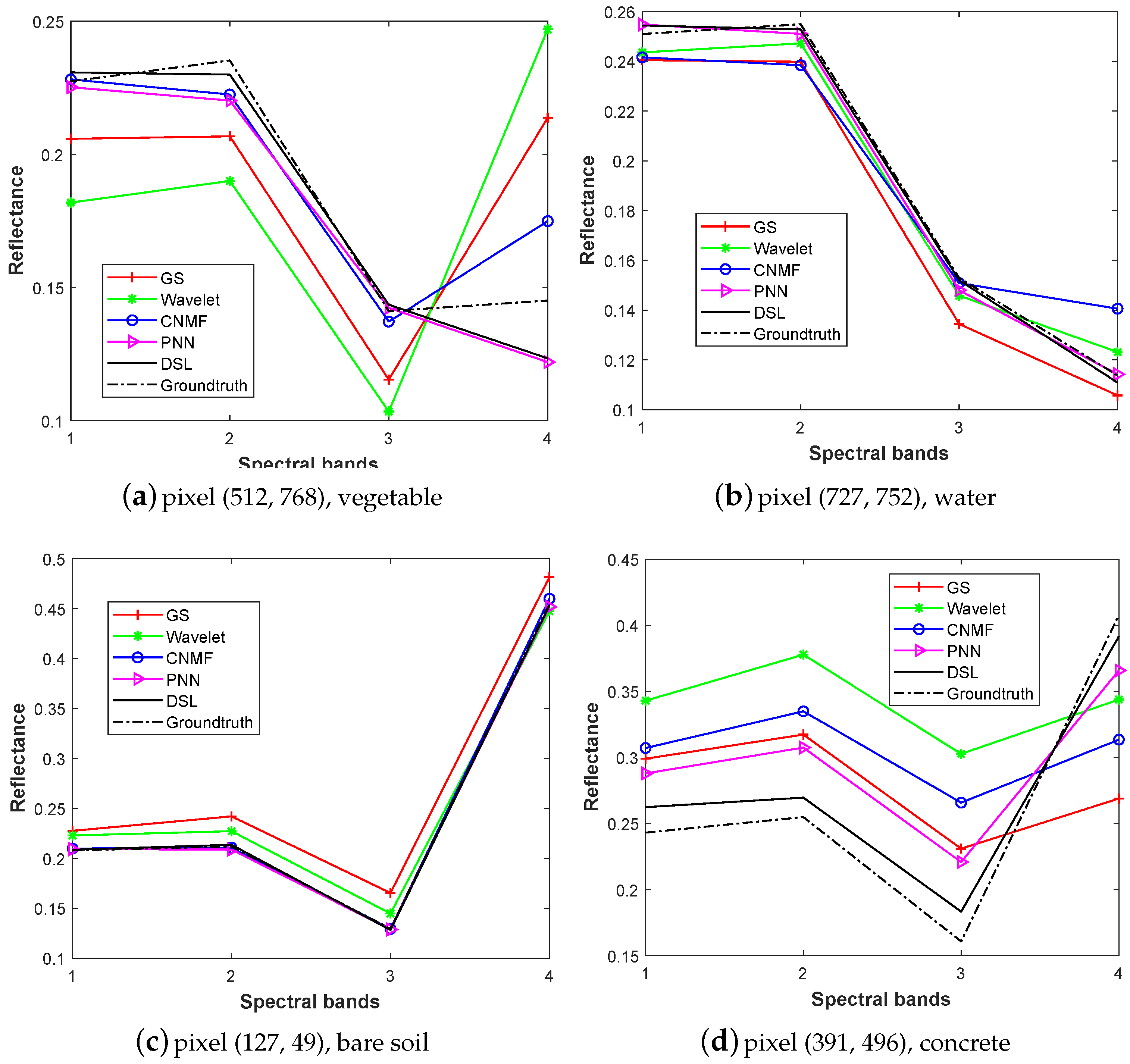
Table 2, Table 3 and Table 4 display the quantitative results of the comparison methods, the best performances are shown in bold. From the results, two observations can be drawn. First, the proposed DSL method obtains the best evaluation results in most of the indexes. For instance, for the three different datasets, the PSNRs of the DSL are 0.45, 0.93, and 0.30 higher than the second-best approach, respectively, demonstrating the great quantitative similarity of the proposed method. In addition, the SSIM of the proposed DSL are significantly higher than the competitors, illustrating the superior spatial consistency of the DSL. Moreover, although the SAM of the DSL scheme is slightly higher than PANNET for the JL-1A dataset, the ERGAS of DSL is lower than the competitors over all three images, demonstrating the effectiveness in the spectral preservation. Furthermore, the spectral curves of four pixels for the GF-1 results are displayed in Figure 9. They are located in (512, 768), (727, 752), (127, 49), and (391, 496) for (x, y) coordinates, and they denote vegetable, water, bare soil, and concrete, respectively. From the spectral signatures, we can find that the proposed DSL obtains the most similar spectral curves to the ground-truth, whatever the object characteristic is. Moreover, it can be observed that the spectral similarities of water and bare soil are higher than the vegetable and the concrete. The above analyses indicate the effectiveness of our DSL no matter in the spatial or spectral domain. Second, it can be observed that DL-based methods obtain deteriorated performance when they are trained on the default wrong kernels. From Table 2, their results are even worse than many of the traditional CS approaches (i.e., PCA and GS), demonstrating the significance of using the right PSF for the DL methods. In addition, the execution time of the DL algorithms is much more than others, even in the GPU environments. The DSL costs less training time than DRPNN and PANNET. This is because the proposed DSL adopts a simpler network structure to learn the nonlinear mapping, rather than the burdensome architecture.
3.3.2. Effectiveness of PSF Estimation Method
From the abovementioned analysis, the PSF exerts significant influence on the performance of the fusion model. If the estimated kernel deviates from the true one, the fusion result can be devastatingly deteriorated. Thus, before comparing the results of the pansharpening, we should assess the effectiveness of the kernel prediction. However, it is difficult to directly compare the proposed algorithm with other PSF estimation methods. On the one hand, the proposed method can be regarded as an unsupervised technique without using the clearer MSI counterpart but, in the literature, the number of unsupervised kernel estimation methods is limited. On the other hand, the codes of most of the unsupervised methods such as [57,58] are unfortunately not publicly available.
Therefore, the effectiveness of our proposed PSF method is evaluated from two aspects. First, we display the overall accuracy of the kernel prediction results for the three datasets. In order to achieve this, we slice the MSI to the small patches and use the trained CNN-1 to predict each of them. Then, we use the overall accuracy (OA) metrics to validate the result. Notice that with the strategy, the true PSF can be obtained as long as more than 50% of the patches can be correctly estimated. The OAs of the prediction results for the three datasets are displayed in Table 5. From the results, we can observe that the method achieves 92.86%, 90.84%, and 56.17% of the OA for the GF-2, GF-1, and JL-1A dataset, respectively, demonstrating that the proposed algorithm can obtain the true kernels over all three datasets. This result indicates the effectiveness of the CNN-1 in kernel estimation.
Second, the effectiveness of the PSF estimation is also demonstrated by comparing the DSL results using the default kernel. The experiment setting is set the same as our DSL model, except the adopted blur kernel. The results are displayed in Table 6. It can be observed that the performance of our PSF estimation significantly surpasses the competitors. For instance, the PSNR of three datasets using our algorithm is 4.00, 1.85, and 1.19 higher than the method using the default kernel, respectively. Therefore, we can draw the conclusion that our PSF estimation method plays an essential role in the image pansharpening.
3.3.3. Comparison with Image Registration Methods
In order to investigate the effectiveness of our edge-based image registration method, we compare our method with other local registration algorithms. Since it is difficult to directly compare the performances of the image registration, we use the pansharpening results of DSL model to illustrate the efficacy of different methods. The comparison method we use is from [44] (we denote it as Aiazzi’s). It is beneficial to recover the local misalignments for the CS- and MTF-based algorithms, however, it has not been used in DL domain. Furthermore, we also set the experiments without the local registration (using the original coarse centroid). Table 7, Table 8 and Table 9 show the results of different local registration methods for the three datasets. It can be observed that the proposed edge-based method obtains the best performance, which illustrates the effectiveness of our registration algorithm. Furthermore, for GF-2 and GF-1 datasets, our method achieves slightly better results than the Aiazzi’s. However, for JL-1A dataset, Aiazzi’s method is seriously deteriorated. The reason is that the method is not suitable for the seriously blurry images. On the contrary, our method can provide the satisfactory results in any condition.
4. Discussion
4.1. Impacts of Image Patch Size
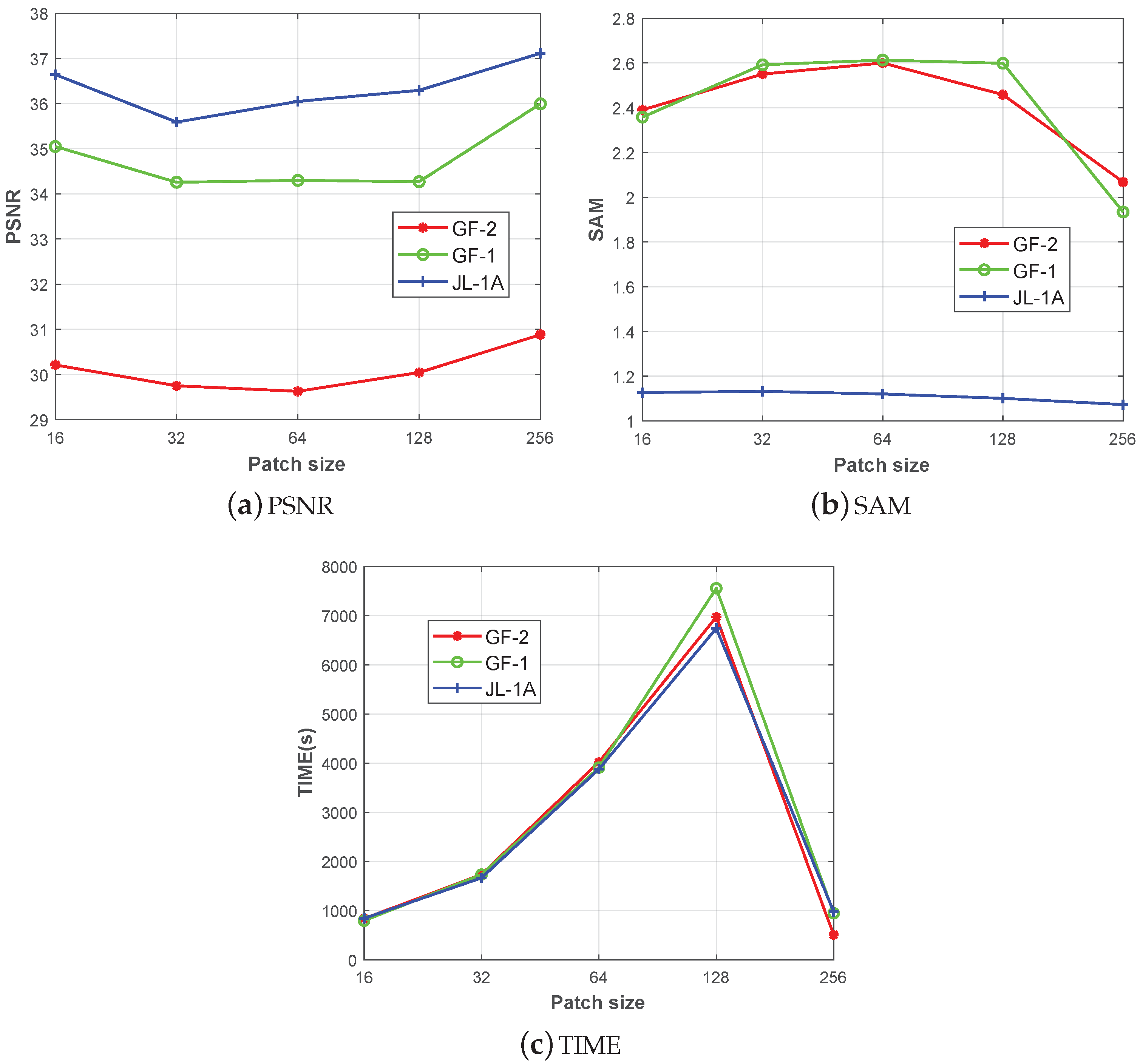
Image patch size is an important parameter for the pansharpening result, due to the learning efficiency and the feature learning that it brings. In this paper, we investigate the impact of the patch size to the experimental result for the three datasets. The patch sizes of the comparison methods are set as , , , and , respectively. For the patch generation, the overlapped number of pixels of each two adjacent patches is set as 8, and the number of the generated samples is then be 961, 861, 625, 289 and 1. For the comparison methods, the batch size is set as 64 and other parameters are set as Section 3.2 in the training stage. The PSNR, SAM and the training time are displayed in Figure 10. It can be observed that the experiment with the size can get the best results and it spends the least training time. It is because that although the patch size is the largest, the extremely small number of training sample accelerates the training procedure. Based on the above analysis, the patch size of the original pixels with no slices is adopted in our experiment.
4.2. Impacts of Training Epochs
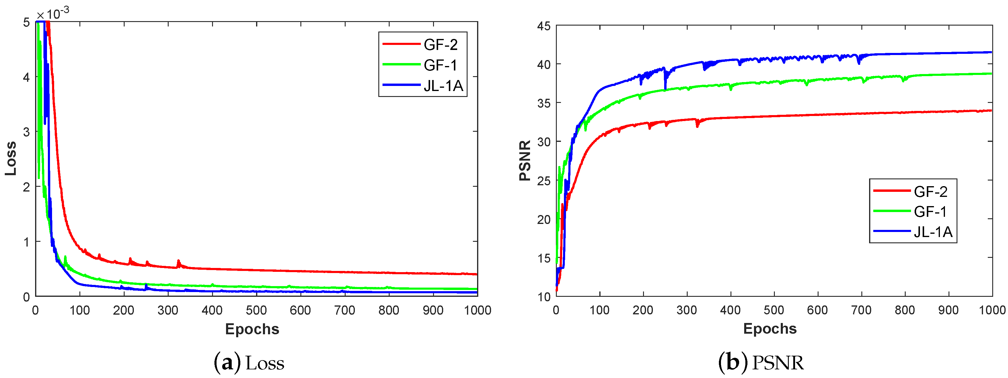
To investigate the speed of the training procedure of the CNN-2 pansharpening model, we display the training curves over time for the three datasets in Figure 11. From the learning curves, the loss declines drastically and fusion model converges rapidly to the fine performance during 100 epochs for the three datasets. After 300 epochs, the loss decreases more slowly but the model is still being fine-tuned. Therefore, to achieve the best performance for the DSL pansharpening model, the epoch number is set to be 1000 in our experiments.
5. Conclusions
In this paper, we have proposed a deep self-learning method (i.e., DSL) for image pansharpening. The main advantage of DSL is that it can explore the PSF from the MSI and PAN and construct the training samples according to the learned degradation. As such, the pansharpening model can adaptively learn the true degradation for any given data. In addition, this model takes the local misalignments between the MSI and PAN into consideration, and they are recovered by the proposed edge-based image registration method. Extensive experiments conducted on three images from different satellites indicate that the proposed DSL obtains good results in the spatial fidelity and the spectral preservation. In the future, we will investigate the nonparametric method for the PSF estimation, which can be more flexible for the pansharpening in practice. Additionally, we will develop the combination of image fusion and image super-resolution to yield better reconstruction results, where the PSF can be used to improve the image quality for MSI.
Author Contributions
All coauthors made significant contributions to the manuscript. J.H. and Z.H. designed the research framework, analyzed the results, and wrote the paper. J.W. assisted in the preparing work and validation work.
Funding
This work is supported in part by the National Key R&D Program of China under Grant Nos. 2018YFB0505500 and 2018YFB0505503, the Fundamental Research Funds for the Central Universities under Grant No. 19lgzd10, and the National Natural Science Foundation of China under Grant Nos. 41501368 and 41531178.
Conflicts of Interest
The authors declare no conflict of interest.
References
- Qu, Y.; Qi, H.; Kwan, C. Unsupervised sparse Dirichlet-net for hyperspectral image super-resolution. In Proceedings of the IEEE Conference on Computer Vision and Pattern Recognition, Lake City, UT, USA, 18–22 June 2018; pp. 2511–2520. [Google Scholar]
- He, Z.; Li, J.; Liu, K.; Liu, L.; Tao, H. Kernel Low-Rank Multitask Learning in Variational Mode Decomposition Domain for Multi-/Hyperspectral Classification. IEEE Trans. Geosci. Remote Sens. 2018, 56, 4193–4208. [Google Scholar] [CrossRef]
- Chen, B.; Huang, B.; Xu, B. Multi-source remotely sensed data fusion for improving land cover classification. ISPRS J. Photogramm. Remote Sens. 2017, 124, 27–39. [Google Scholar] [CrossRef]
- Matteoli, S.; Diani, M.; Corsini, G. Automatic target recognition within anomalous regions of interest in hyperspectral images. IEEE J. Sel. Top. Appl. Earth Obs. Remote Sens. 2018, 11, 1056–1069. [Google Scholar] [CrossRef]
- Murray, N.J.; Keith, D.A.; Simpson, D.; Wilshire, J.H.; Lucas, R.M. Remap: An online remote sensing application for land cover classification and monitoring. Methods Ecol. Evol. 2018, 9, 2019–2027. [Google Scholar] [CrossRef]
- Liu, Z.; Li, G.; Mercier, G.; He, Y.; Pan, Q. Change detection in heterogenous remote sensing images via homogeneous pixel transformation. IEEE Trans. Image Process. 2018, 27, 1822–1834. [Google Scholar] [CrossRef] [PubMed]
- Shahdoosti, H.R.; Ghassemian, H. Combining the spectral PCA and spatial PCA fusion methods by an optimal filter. Inform. Fusion 2016, 27, 150–160. [Google Scholar] [CrossRef]
- Carper, W.; Littlesand, T.; Kiefer, R. The use of intensity-hue-saturation transformations for merging SPOT panchromatic and multispectral image data. Photogramm. Eng. Remote Sens. 1990, 56, 459–467. [Google Scholar]
- Aiazzi, B.; Baronti, S.; Selva, M. Improving component substitution pansharpening through multivariate regression of MS + Pan data. IEEE Trans. Geosci. Remote Sens. 2007, 45, 3230–3239. [Google Scholar] [CrossRef]
- Maglione, P.; Parente, C.; Vallario, A. Pan-sharpening Worldview-2: IHS, Brovey and Zhang methods in comparison. Int. J. Eng. Technol. 2016, 8, 673–679. [Google Scholar]
- Zhang, Y.; De Backer, S.; Scheunders, P. Noise-resistant wavelet-based Bayesian fusion of multispectral and hyperspectral images. IEEE Trans. Geosci. Remote Sens. 2009, 47, 3834–3843. [Google Scholar] [CrossRef]
- Shensa, M.J. The discrete wavelet transform: Wedding the à trous and Mallat algorithms. IEEE Trans. Signal Process. 1992, 40, 2464–2482. [Google Scholar] [CrossRef]
- Burt, P.; Adelson, E. The Laplacian pyramid as a compact image code. IEEE Trans. Commun. 1983, 31, 532–540. [Google Scholar] [CrossRef]
- Do, M.N.; Vetterli, M. The contourlet transform: An efficient directional multiresolution image representation. IEEE Trans. Image Process. 2005, 14, 2091–2106. [Google Scholar] [CrossRef] [PubMed]
- Liao, W.; Huang, X.; Coillie, F.V.; Gautama, S.; Pizurica, A.; Philips, W.; Liu, H.; Zhu, T.; Shimoni, M.; Moser, G.; et al. Processing of Multiresolution Thermal Hyperspectral and Digital Color Data: Outcome of the 2014 IEEE GRSS Data Fusion Contest. IEEE J. Sel. Topics Appl. Earth Observ. Remote Sens. 2015, 8, 2984–2996. [Google Scholar] [CrossRef]
- Li, Z.; Jing, Z.; Yang, X.; Sun, S. Color transfer based remote sensing image fusion using non-separable wavelet frame transform. Pattern. Recog. Lett. 2005, 26, 2006–2014. [Google Scholar] [CrossRef]
- Loncan, L.; De Almeida, L.B.; Bioucas-Dias, J.M.; Briottet, X.; Chanussot, J.; Dobigeon, N.; Fabre, S.; Liao, W.; Licciardi, G.A.; Simoes, M.; et al. Hyperspectral pansharpening: A review. IEEE Geosci. Remote Sens. Mag. 2015, 3, 27–46. [Google Scholar] [CrossRef]
- Khademi, G.; Ghassemian, H. Incorporating an Adaptive Image Prior Model Into Bayesian Fusion of Multispectral and Panchromatic Images. IEEE Geosci. Remote Sens. Lett. 2018, 15, 917–921. [Google Scholar] [CrossRef]
- Huang, B.; Song, H.; Cui, H.; Peng, J.; Xu, Z. Spatial and spectral image fusion using sparse matrix factorization. IEEE Trans. Geosci. Remote Sens. 2014, 52, 1693–1704. [Google Scholar] [CrossRef]
- Guo, M.; Zhang, H.; Li, J.; Zhang, L.; Shen, H. An online coupled dictionary learning approach for remote sensing image fusion. IEEE J. Sel. Top. Appl. Earth Observ. Remote Sens. 2014, 7, 1284–1294. [Google Scholar] [CrossRef]
- Simões, M.; Bioucas-Dias, J.; Almeida, L.B.; Chanussot, J. A convex formulation for hyperspectral image superresolution via subspace-based regularization. IEEE Trans. Geosci. Remote Sens. 2015, 53, 3373–3388. [Google Scholar] [CrossRef]
- Zou, Q.; Ni, L.; Zhang, T.; Wang, Q. Deep learning based feature selection for remote sensing scene classification. IEEE Geosci. Remote Sens. Lett. 2015, 12, 2321–2325. [Google Scholar] [CrossRef]
- Chen, Y.; Tai, Y.; Liu, X.; Shen, C.; Yang, J. Fsrnet: End-to-end learning face super-resolution with facial priors. In Proceedings of the IEEE Conference on Computer Vision and Pattern Recognition, Lake City, UT, USA, 18–22 June 2018; pp. 2492–2501. [Google Scholar]
- Yuan, Y.; Zheng, X.; Lu, X. Hyperspectral image superresolution by transfer learning. IEEE J. Sel. Top. Appl. Earth Obs. 2017, 10, 1963–1974. [Google Scholar] [CrossRef]
- Schroff, F.; Kalenichenko, D.; Philbin, J. Facenet: A unified embedding for face recognition and clustering. In Proceedings of the IEEE Conference on Computer Vision and Pattern Recognition, Boston, MA, USA, 7–12 June 2015; pp. 815–823. [Google Scholar]
- Dian, R.; Li, S.; Guo, A.; Fang, L. Deep hyperspectral image sharpening. IEEE Trans. Neur. Net. Lear. 2018, 29, 5345–5355. [Google Scholar] [CrossRef] [PubMed]
- Huang, W.; Xiao, L.; Wei, Z.; Liu, H.; Tang, S. A new pan-sharpening method with deep neural networks. IEEE Geosci. Remote Sens. Lett. 2015, 12, 1037–1041. [Google Scholar] [CrossRef]
- Dong, C.; Loy, C.C.; He, K.; Tang, X. Image super-resolution using deep convolutional networks. IEEE Trans. Pattern Anal. Mach. Intell. 2016, 38, 295–307. [Google Scholar] [CrossRef]
- Dong, C.; Loy, C.C.; He, K.; Tang, X. Learning a deep convolutional network for image super-resolution. In Proceedings of the European Conference on Computer Vision, Zuerich, Switzerland, 5–12 September 2014; pp. 184–199. [Google Scholar]
- Masi, G.; Cozzolino, D.; Verdoliva, L.; Scarpa, G. Pansharpening by convolutional neural networks. Remote Sens. 2016, 8, 594. [Google Scholar] [CrossRef]
- Rao, Y.; He, L.; Zhu, J. A residual convolutional neural network for pan-shaprening. In Proceedings of the 2017 International Workshop on Remote Sensing with Intelligent Processing (RSIP), Shanghai, China, 19–21 May 2017; pp. 1–4. [Google Scholar]
- Wei, Y.; Yuan, Q.; Shen, H.; Zhang, L. Boosting the Accuracy of Multispectral Image Pansharpening by Learning a Deep Residual Network. IEEE Geosci. Remote Sens. Lett. 2017, 14, 1795–1799. [Google Scholar] [CrossRef] [Green Version]
- Song, H.; Liu, Q.; Wang, G.; Hang, R.; Huang, B. Spatiotemporal satellite image fusion using deep convolutional neural networks. IEEE J. Sel. Top. Appl. Earth Obs. 2018, 11, 821–829. [Google Scholar] [CrossRef]
- Liu, X.; Wang, Y.; Liu, Q. Psgan: A Generative Adversarial Network for Remote Sensing Image Pan-Sharpening. In Proceedings of the IEEE International Conference on Image Processing (ICIP), Athens, Greece, 7–10 October 2018; pp. 873–877. [Google Scholar]
- Palsson, F.; Sveinsson, J.R.; Ulfarsson, M.O. Multispectral and Hyperspectral Image Fusion Using a 3-D-Convolutional Neural Network. IEEE Geosci. Remote Sens. Lett. 2017, 14, 639–643. [Google Scholar] [CrossRef]
- Liu, X.; Wang, Y.; Liu, Q. Remote Sensing Image Fusion Based on Two-stream Fusion Network. In Proceedings of the 2018 International Conference on Multimedia Modeling, Bangkok, Thailand, 3–17 November 2018; pp. 428–439. [Google Scholar]
- Yang, J.; Fu, X.; Hu, Y.; Huang, Y.; Ding, X.; Paisley, J. PanNet: A deep network architecture for pan-sharpening. In Proceedings of the IEEE International Conference on Computer Vision, Venice, Italy, 22–29 October 2017; pp. 1753–1761. [Google Scholar]
- Xing, Y.; Wang, M.; Yang, S.; Jiao, L. Pan-sharpening via deep metric learning. ISPRS J. Photogramm. Remote Sens. 2018, 145, 165–183. [Google Scholar] [CrossRef]
- Azarang, A.; Ghassemian, H. A new pansharpening method using multi resolution analysis framework and deep neural networks. In Proceedings of the International Conference on Pattern Recognition and Image Analysis (IPRIA), Shahrekord, Iran, 19–20 April 2017; pp. 1–6. [Google Scholar]
- Zhong, J.; Yang, B.; Huang, G.; Zhong, F.; Chen, Z. Remote sensing image fusion with convolutional neural network. Sens. Imaging 2016, 17, 1–16. [Google Scholar] [CrossRef]
- Lanaras, C.; Bioucas-Dias, J.; Galliani, S.; Baltsavias, E.; Schindler, K. Super-resolution of Sentinel-2 images: Learning a globally applicable deep neural network. ISPRS J. Photogramm. Remote Sens. 2018, 146, 305–319. [Google Scholar] [CrossRef] [Green Version]
- Shocher, A.; Cohen, N.; Irani, M. “Zero-shot” Super-Resolution using Deep Internal Learning. In Proceedings of the IEEE Conference on Computer Vision and Pattern Recognition, Lake City, UT, USA, 18–22 June 2018; pp. 3118–3126. [Google Scholar]
- Ballester, C.; Caselles, V.; Igual, L.; Verdera, J.; Rougé, B. A Variational Model for P + XS Image Fusion. Int. J. Comput. Vis. 2006, 69, 43–58. [Google Scholar] [CrossRef]
- Aiazzi, B.; Alparone, L.; Garzelli, A.; Santurri, L. Blind correction of local misalignments between multispectral and panchromatic images. IEEE Geosci. Remote Sens. Lett. 2018, 15, 1625–1629. [Google Scholar] [CrossRef]
- Krizhevsky, A.; Sutskever, I.; Hinton, G.E. ImageNet Classification with Deep Convolutional Neural Networks. In Proceedings of the Advances in Neural Information Processing Systems, Lake Tahoe, NV, USA, 3–6 December 2012; pp. 1097–1105. [Google Scholar]
- Dahl, G.E.; Sainath, T.N.; Hinton, G.E. Improving deep neural networks for LVCSR using rectified linear units and dropout. In Proceedings of the 2013 IEEE International Conference on Acoustics, Speech and Signal Processing, Vancouver, BC, Canada, 26–31 May 2013; pp. 8609–8613. [Google Scholar]
- Liu, W.; Wen, Y.; Yu, Z.; Yang, M.M. Large-margin softmax loss for convolutional neural networks. In Proceedings of the 33rd International Conference on International Conference on Machine Learning, New York, NY, USA, 19–24 June 2016; pp. 507–516. [Google Scholar]
- Chen, F.; Ma, J. An empirical identification method of gaussian blur parameter for image deblurring. IEEE Trans. Image Process. 2009, 57, 2467–2478. [Google Scholar] [CrossRef]
- Ding, L.; Goshtasby, A. On the Canny edge detector. Pattern Recognit. 2001, 34, 721–725. [Google Scholar] [CrossRef]
- Kwan, C.; Choi, J.H.; Chan, S.H.; Zhou, J.; Budavari, B. A super-resolution and fusion approach to enhancing hyperspectral images. Remote Sens. 2018, 10, 1416. [Google Scholar] [CrossRef]
- Chan, S.H.; Wang, X.; Elgendy, O.A. Plug-and-play ADMM for image restoration: Fixed-point convergence and applications. IEEE Trans. Comput. Imaging 2017, 3, 84–98. [Google Scholar] [CrossRef]
- Krishnan, D.; Fergus, R. Fast image deconvolution using hyper-Laplacian priors. In Proceedings of the Advances in Neural Information Processing Systems (NIPS), Vancouver, BC, Canada, 7–10 December 2009; pp. 1033–1041. [Google Scholar]
- Aiazzi, B.; Alparone, L.; Baronti, S.; Garzelli, A.; Selva, M. MTF-tailored multiscale fusion of high-resolution MS and pan imagery. ISPRS J. Photogramm. Remote Sens. 2006, 72, 591–596. [Google Scholar] [CrossRef]
- King, R.L.; Wang, J. A wavelet based algorithm for pan sharpening Landsat 7 imagery. In Proceedings of the 2001 IEEE International Geoscience and Remote Sensing Symposium (IGARSS), Sydney, Australia, 9–13 July 2001; Volume 2, pp. 849–851. [Google Scholar]
- Yokoya, N.; Yairi, T.; Iwasaki, A. Coupled nonnegative matrix factorization unmixing for hyperspectral and multispectral data fusion. IEEE Trans. Geosci. Remote Sens. 2012, 50, 528–537. [Google Scholar] [CrossRef]
- Wei, Y.; Yuan, Q. Deep residual learning for remote sensed imagery pansharpening. In Proceedings of the 2017 International Workshop on Remote Sensing with Intelligent Processing (RSIP), Shanghai, China, 19–21 May 2017; pp. 1–4. [Google Scholar]
- Michaeli, T.; Irani, M. Nonparametric blind super-resolution. In Proceedings of the IEEE International Conference on Computer Vision, Sydney, Australia, 1–8 December 2013; pp. 945–952. [Google Scholar]
- Shao, W.Z.; Elad, M. Simple, accurate, and robust nonparametric blind super-resolution. In Proceedings of the International Conference on Image and Graphics, Tianjin, China, 13–15 August 2015; pp. 333–348. [Google Scholar]
Figure 1.
Flowchart of the proposed deep self-learning (DSL) architecture.

Figure 2.
Structure of the proposed CNN-1 for point spread function (PSF) estimation.

Figure 3.
Blur kernel with different , and the blurred results using the GF-2 satellite image and the corresponding blur kernels. The blur region is fixed as 21 × 21.
Figure 3.
Blur kernel with different , and the blurred results using the GF-2 satellite image and the corresponding blur kernels. The blur region is fixed as 21 × 21.

Figure 4.
Structure of the proposed CNN-2 for the pansharpening.

Figure 5.
Three remotely sensed images used in the experiments. (a–c) depict panchromatic images (PAN) images. Multispectral images (MSI) images with the red, green, and blue channels are displayed in (d–f), respectively.
Figure 5.
Three remotely sensed images used in the experiments. (a–c) depict panchromatic images (PAN) images. Multispectral images (MSI) images with the red, green, and blue channels are displayed in (d–f), respectively.

Figure 6.
Pansharpening results for GF-2 dataset. Results best viewed electronically with zoom.

Figure 7.
Pansharpening results for GF-1 dataset. Results best viewed electronically with zoom.

Figure 8.
Pansharpening results for JL-1A dataset. Results best viewed electronically with zoom.

Figure 9.
Spectral signatures of four pixels for the GF-1 dataset.

Figure 10.
PSNR, SAM, and execution time for different patch sizes for the three datasets.

Figure 11.
Training loss and PSNR evolution for the three datasets.


Table 1.
Comparison methods considered in the experiments.
| Abbreviation | Description | Reference |
|---|---|---|
| PCA | Principle component analysis | [17] |
| GS | Gram–Schmidt algorithm | [9] |
| MTF-GLP | Generalized Laplacian pyramid algorithm | [53] |
| Wavelet | Wavelet transform | [54] |
| CNMF | Coupled non-negative matrix factorization | [55] |
| PNN | Pansharpening by convolutional neural networks | [30] |
| DRPNN | Deep residual learning for pansharpening | [56] |
| PANNET | Pansharpening by deep network | [37] |
| DSL | The proposed deep self-learning for pansharpening | - |
Table 2.
Quantitative results of the comparison pansharpening methods for the GF-2 dataset. Bold values indicate the best result for a column.
Table 2.
Quantitative results of the comparison pansharpening methods for the GF-2 dataset. Bold values indicate the best result for a column.
| Methods | RMSE | PSNR | SSIM | SAM | CC | ERGAS | Execution Time |
|---|---|---|---|---|---|---|---|
| PCA | 0.042 | 27.55 | 0.94 | 3.04 | 0.92 | 3.32 | 1.31 s (CPU) |
| GS | 0.039 | 28.22 | 0.95 | 2.88 | 0.94 | 3.08 | 0.86 s (CPU) |
| MTF-GLP | 0.030 | 30.43 | 0.96 | 2.06 | 0.97 | 2.37 | 0.95 s (CPU) |
| Wavelet | 0.048 | 26.44 | 0.92 | 3.03 | 0.89 | 3.84 | 1.22 s (CPU) |
| CNMF | 0.032 | 29.80 | 0.96 | 2.86 | 0.95 | 2.51 | 11.47 s (CPU) |
| PNN | 0.043 | 27.20 | 0.92 | 2.53 | 0.93 | 3.50 | 1277.50 s (GPU) |
| DRPNN | 0.051 | 25.93 | 0.90 | 3.41 | 0.92 | 4.10 | 2082.92 s (GPU) |
| PANNET | 0.044 | 27.11 | 0.94 | 2.89 | 0.91 | 3.55 | 1614.02 s (GPU) |
| DSL | 0.029 | 30.88 | 0.96 | 2.07 | 0.97 | 2.31 | 1506.83 s (GPU) |
Table 3.
Quantitative results of the comparison pansharpening methods for the GF-1 dataset. Bold values indicate the best result for a column.
Table 3.
Quantitative results of the comparison pansharpening methods for the GF-1 dataset. Bold values indicate the best result for a column.
| Methods | RMSE | PSNR | SSIM | SAM | CC | ERGAS | Execution Time |
|---|---|---|---|---|---|---|---|
| PCA | 0.030 | 30.51 | 0.91 | 4.00 | 0.87 | 2.84 | 3.67 s (CPU) |
| GS | 0.025 | 32.11 | 0.95 | 3.09 | 0.88 | 2.68 | 1.22 s (CPU) |
| MTF-GLP | 0.018 | 35.06 | 0.96 | 1.92 | 0.94 | 1.90 | 1.05 s (CPU) |
| Wavelet | 0.027 | 31.45 | 0.91 | 3.53 | 0.85 | 2.80 | 1.73 s (CPU) |
| CNMF | 0.019 | 34.65 | 0.96 | 2.66 | 0.92 | 2.00 | 11.34 s (CPU) |
| PNN | 0.017 | 35.25 | 0.96 | 2.21 | 0.95 | 1.80 | 860.30 s (GPU) |
| DRPNN | 0.020 | 34.10 | 0.95 | 2.51 | 0.94 | 2.10 | 996.49 s (GPU) |
| PANNET | 0.022 | 33.35 | 0.95 | 2.91 | 0.94 | 2.28 | 1829.33 s (GPU) |
| DSL | 0.016 | 35.99 | 0.97 | 1.93 | 0.95 | 1.67 | 946.95 s (GPU) |
Table 4.
Quantitative results of the comparison pansharpening methods for the JL-1A dataset. Bold values indicate the best result for a column.
Table 4.
Quantitative results of the comparison pansharpening methods for the JL-1A dataset. Bold values indicate the best result for a column.
| Methods | RMSE | PSNR | SSIM | SAM | CC | ERGAS | Execution Time |
|---|---|---|---|---|---|---|---|
| PCA | 0.039 | 28.22 | 0.93 | 3.04 | 0.62 | 3.71 | 0.47 s (CPU) |
| GS | 0.038 | 28.33 | 0.93 | 2.99 | 0.63 | 3.66 | 0.59 s (CPU) |
| MTF-GLP | 0.014 | 36.81 | 0.97 | 1.06 | 0.95 | 1.37 | 1.46 s (CPU) |
| Wavelet | 0.018 | 34.46 | 0.96 | 1.08 | 0.98 | 1.80 | 0.94 s (CPU) |
| CNMF | 0.028 | 30.96 | 0.96 | 1.95 | 0.77 | 2.63 | 8.23 s (CPU) |
| PNN | 0.016 | 35.65 | 0.97 | 1.17 | 0.94 | 1.56 | 790.09 s (GPU) |
| DRPNN | 0.016 | 36.02 | 0.97 | 1.08 | 0.94 | 1.50 | 1452.06 s (GPU) |
| PANNET | 0.016 | 35.95 | 0.97 | 0.99 | 0.94 | 1.52 | 1516.01 s (GPU) |
| DSL | 0.014 | 37.11 | 0.97 | 1.07 | 0.95 | 1.31 | 976.61 s (GPU) |
Table 5.
Overall accuracies (OA) of the blur kernel estimation method for the three datasets.
| Data | GF-2 | GF-1 | JL-1A |
|---|---|---|---|
| OA | 92.86% | 90.84% | 56.17% |
Table 6.
The comparison results of the DSL with PSF estimation and with the default kernel.
| Data | PSF Estimation | Default Kernel | ||||||||
|---|---|---|---|---|---|---|---|---|---|---|
| PSNR | SSIM | SAM | CC | ERGAS | PSNR | SSIM | SAM | CC | ERGAS | |
| GF-2 | 30.88 | 0.96 | 2.07 | 0.97 | 2.31 | 26.88 | 0.92 | 2.80 | 0.93 | 3.66 |
| GF-1 | 35.99 | 0.97 | 1.93 | 0.95 | 1.67 | 34.14 | 0.95 | 2.45 | 0.94 | 2.07 |
| JL-1A | 37.11 | 0.97 | 1.07 | 0.95 | 1.31 | 35.92 | 0.97 | 1.01 | 0.94 | 1.51 |
Table 7.
The comparison results of the DSL with different local registration methods for GF-2 dataset.
Table 7.
The comparison results of the DSL with different local registration methods for GF-2 dataset.
| Methods | PSNR | SSIM | SAM | CC | ERGAS |
|---|---|---|---|---|---|
| Proposed | 30.88 | 0.96 | 2.07 | 0.97 | 2.31 |
| Aiazzi’s | 30.04 | 0.96 | 2.27 | 0.96 | 2.58 |
| Without registration | 26.00 | 0.91 | 2.61 | 0.89 | 4.03 |
Table 8.
The comparison results of the DSL with different local registration methods for GF-1 dataset.
Table 8.
The comparison results of the DSL with different local registration methods for GF-1 dataset.
| Methods | PSNR | SSIM | SAM | CC | ERGAS |
|---|---|---|---|---|---|
| Proposed | 35.99 | 0.97 | 1.93 | 0.95 | 1.67 |
| Aiazzi’s | 33.89 | 0.95 | 2.62 | 0.94 | 1.99 |
| Without registration | 32.49 | 0.93 | 2.55 | 0.96 | 2.35 |
Table 9.
The comparison results of the DSL with different local registration methods for JL-1A dataset.
Table 9.
The comparison results of the DSL with different local registration methods for JL-1A dataset.
| Methods | PSNR | SSIM | SAM | CC | ERGAS |
|---|---|---|---|---|---|
| Proposed | 37.11 | 0.97 | 1.07 | 0.95 | 1.31 |
| Aiazzi’s | 22.67 | 0.78 | 4.97 | 0.61 | 6.97 |
| Without registration | 36.42 | 0.97 | 1.00 | 0.95 | 1.43 |
© 2019 by the authors. Licensee MDPI, Basel, Switzerland. This article is an open access article distributed under the terms and conditions of the Creative Commons Attribution (CC BY) license (http://creativecommons.org/licenses/by/4.0/).
Share and Cite
MDPI and ACS Style
Hu, J.; He, Z.; Wu, J. Deep Self-Learning Network for Adaptive Pansharpening. Remote Sens. 2019, 11, 2395. https://0-doi-org.brum.beds.ac.uk/10.3390/rs11202395
AMA Style
Hu J, He Z, Wu J. Deep Self-Learning Network for Adaptive Pansharpening. Remote Sensing. 2019; 11(20):2395. https://0-doi-org.brum.beds.ac.uk/10.3390/rs11202395
Chicago/Turabian StyleHu, Jie, Zhi He, and Jiemin Wu. 2019. "Deep Self-Learning Network for Adaptive Pansharpening" Remote Sensing 11, no. 20: 2395. https://0-doi-org.brum.beds.ac.uk/10.3390/rs11202395
Note that from the first issue of 2016, this journal uses article numbers instead of page numbers. See further details here.