Wetland Classification Based on a New Efficient Generative Adversarial Network and Jilin-1 Satellite Image


1
School of Geography and Planning, Guangdong Provincial Key Laboratory of Urbanization and Geo-simulation, Center of Integrated Geographic Information Analysis, Sun Yat-sen University (SYSU), Guangzhou 510275, China
2
City College of Dongguan University of Technology, Dongguan 511700, China
*
Author to whom correspondence should be addressed.
Remote Sens. 2019, 11(20), 2455; https://0-doi-org.brum.beds.ac.uk/10.3390/rs11202455
Submission received: 23 September 2019
/
Revised: 11 October 2019
/
Accepted: 18 October 2019
/
Published: 22 October 2019
Abstract
:Recent studies have shown that deep learning methods provide useful tools for wetland classification. However, it is difficult to perform species-level classification with limited labeled samples. In this paper, we propose a semi-supervised method for wetland species classification by using a new efficient generative adversarial network (GAN) and Jilin-1 satellite image. The main contributions of this paper are twofold. First, the proposed method, namely ShuffleGAN, requires only a small number of labeled samples. ShuffleGAN is composed of two neural networks (i.e., generator and discriminator), which perform an adversarial game in the training phase and ShuffleNet units are added in both generator and discriminator to obtain speed-accuracy tradeoff. Second, ShuffleGAN can perform species-level wetland classification. In addition to distinguishing the wetland areas from non-wetlands, different tree species located in the wetland are also identified, thus providing a more detailed distribution of the wetland land-covers. Experiments are conducted on the Haizhu Lake wetland data acquired by the Jilin-1 satellite. Compared with existing GAN, the improvement in overall accuracy (OA) of the proposed ShuffleGAN is more than 2%. This work can not only deepen the application of deep learning in wetland classification but also promote the study of fine classification of wetland land-covers.
1. Introduction
Wetlands [1], known as “the kidney of the earth,” are highly productive and biodiverse ecosystems that play vital roles in environmental sustainability, and thus, mapping wetlands is crucially important for us to survey the species distribution and analyze the dynamic changes of the wetland area [2,3]. However, it is difficult to carry out research on wetland distribution, especially for species-level classification, because the underlying surface of wetlands is complicated and the acquisition of labeled samples is time-consuming and expensive.
Remote sensing technologies [4] have proven to be effective tools in mapping the wetland distribution. One of the major imagery sources is multispectral data, including Landsat [5,6], Sentinel [7,8] and WorldView [9,10]. Unmanned aerial vehicles (UAV) [11] and hyperspectral sensors [12,13] are also frequently applied in wetland classification over the past few years. Wetland classification applications are advancing, many moving from low and moderate resolution imagery to high resolution.
Intensive classification methods have been proposed to deal with the wetland classification issue. Generally, those methods can fall into three categories, that is, unsupervised, supervised and semi-supervised. Unsupervised methods focus on separating the samples by extracting patterns on its own. Notably no labeled samples are required, the unsupervised methods can be easily used for wetland classification. Typical unsupervised classification methods include k-means cluster [14] and self-organizing maps (SOM) [15]. Unfortunately, it is hard to explore the relationship between clusters and class labels with too little a priori knowledge. Supervised methods, which are extensively used in wetland classification, have received improved performance by making full use of the prior information. A lot of supervised methods, such as support vector machine (SVM) [16,17] and random forest (RF) [18], have been reported in the literature. However, supervised methods always require many labeled samples to train satisfactory classifiers and a large number of unlabeled samples are ignored. Semi-supervised methods train the classifiers by simultaneously utilizing both limited labeled samples and numerous unlabeled samples that can be obtained without additional cost. State-of-the-art semi-supervised methods include the Laplacian SVM (LapSVM) [19,20] and transductive SVM (TSVM) [21]. This kind of method provides an effective strategy to overcome the problem of lacking labeled samples and the research on semi-supervised wetland classification has just began.
Motivated by the rapid development of artificial intelligence (AI), deep learning methods [22,23] have been found to be remarkably effective in the machine learning area and have been introduced to wetland classification since 2018 [24,25,26,27]. Deep learning models can hierarchically learn high-level features with multiple hidden layers. Widely used deep architectures include the deep belief networks (DBNs) [28], stacked autoencoder (SAE) [22], residual network (ResNet) [29] and generative adversarial network (GAN) [30,31]. Among various deep learning methods, convolutional neural networks (CNN) [32] have become a preferable model owing to the fact that the convolution filters in CNN provide efficient tools to automatically extract the spectral-spatial features. For instance, Rezaee et al. [24] introduced the AlexNet to complex wetland mapping and obtained better results than RF. Mahdianpari et al. [25] applied seven well-known deep neural networks for wetland mapping and found that those deep learning methods performed better than conventional machine learning tools (e.g., SVM). Liu and Abd-Elrahman [26] proposed a novel multi-view object-based classification method by using CNN and UAV, their results indicated that CNN provided higher accuracy than traditional classifiers. Moreover, Mohammadimanesh et al. [27] proposed a fully convolutional network (FCN) architecture with an encoder-decoder paradigm for complex land cover mapping of Synthetic Aperture Radar (SAR) images. Notwithstanding the applicableness and successfulness of the deep learning methods mentioned above, their performance still can be improved. On the one hand, almost all the aforementioned wetland classification models motivated by deep learning are supervised, which require massive labeled samples. On the other hand, the research on deep learning-based wetland classification methods is only getting started and the wetland land-covers are rarely separated at detailed levels, especially for species-level classification.
In this paper, an object-based semi-supervised wetland classification method, namely ShuffleGAN, is proposed to address the above-mentioned issues. The proposed method is an efficient GAN trained by using limited labeled samples and many unlabeled samples. Jilin-1 satellite image is applied to record the land-cover information and objects are obtained by the simple linear iterative clustering (SLIC) [33] based superpixel segmentation. ShuffleNet units [34] are added in the network to gain better speed-accuracy tradeoff. To sum up, the main contributions of this work lie in the following two aspects:
- We propose a new GAN architecture (i.e., ShuffleGAN) for wetland classification. The ShuffleGAN is a semi-supervised method, in which only a small number of labeled samples are required. Moreover, the proposed ShuffleGAN is more effective than the traditional GAN since lightweight ShuffleNet units are adopted.
- We perform species-level identification rather than coarse classification (e.g., wetland and non-wetland). Different tree species (e.g., Ficus, Alstonia scholaris and Delonix, etc.) located in the wetland are separated by using the ShuffleGAN and Jilin-1 satellite image. Species-level classification is beneficial to obtain detailed distribution of the wetland vegetation, thus providing more valuable information for finely analyzing the spatiotemporal distribution regularity of various tree species.
The reminder of this paper is organized as follows. In Section 2, we give detailed descriptions of the proposed method. In Section 3, experimental results on Jilin-1 satellite image are reported to compare with other methods. Discussions are shown in Section 4 and conclusions are drawn in Section 5.
2. The Proposed Method
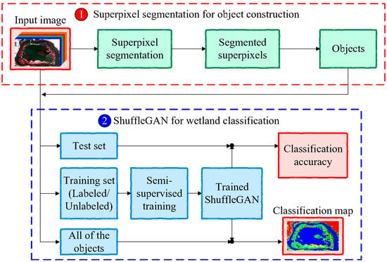
The general procedure of the proposed method is illustrated in Figure 1, which contains two main parts: (1) Superpixel segmentation for object construction. In this step, SLIC algorithm is utilized to segment the input remote sensing image into many superpixels and objects can be subsequently extracted from the input image in accordance with the segmented superpixels. (2) ShuffleGAN for wetland classification. In this step, ShuffleGAN is trained by feeding the training set, which is comprised of both labeled and unlabeled samples. The testing set is classified by the trained ShuffleGAN so as to obtain the classification accuracy and the classification map can be finally generated by classifying all of the objects in the whole scene.
2.1. Superpixel Segmentation for Object Construction
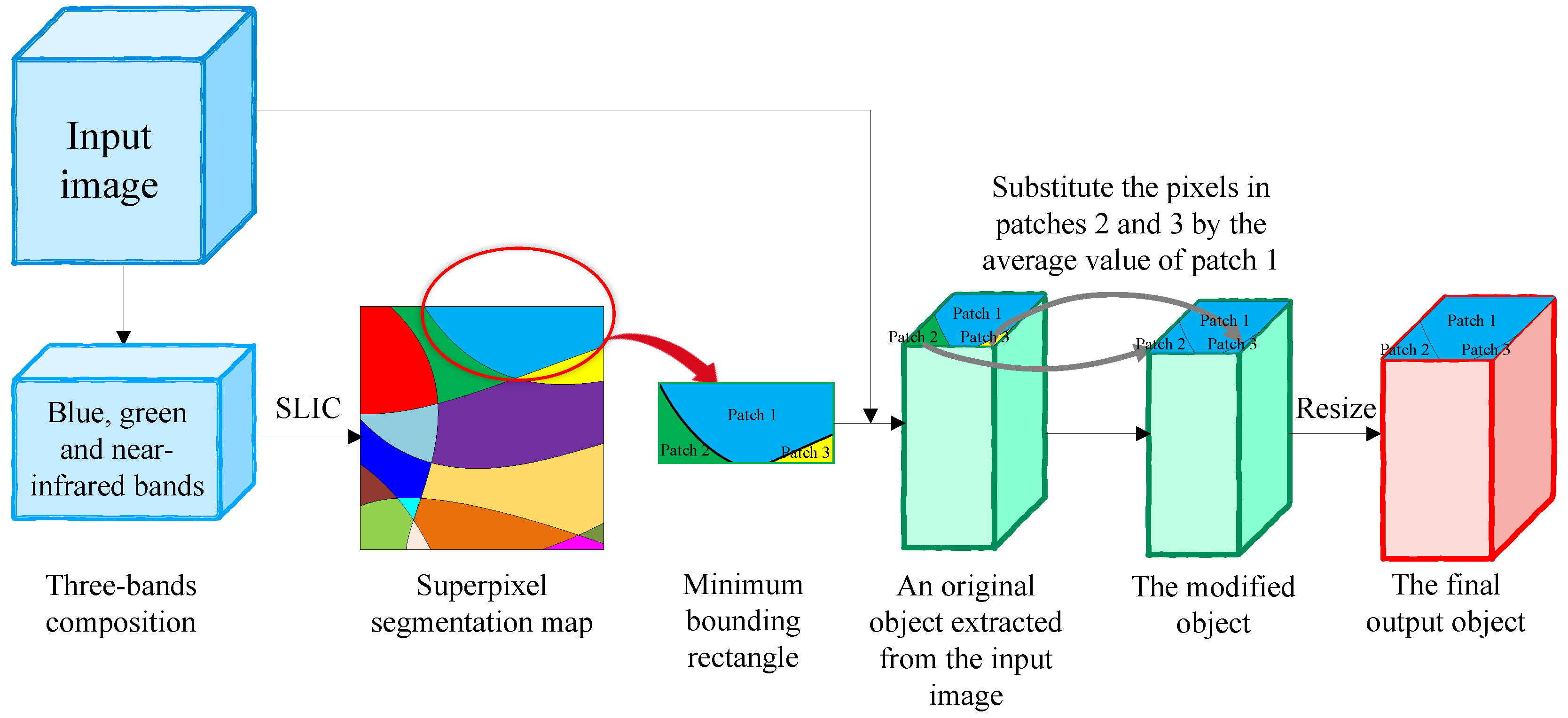
Figure 2 gives a schematic illustration of object construction. We perform SLIC-based superpixel segmentation on the three-bands composition (i.e., blue, green and near-infrared bands) of the input image to obtain the over-segmented map. The SLIC method, which is taken as an adaption of k-means clustering, has proved to be very useful for over-segmenting an RGB or gray-scale image into homogeneous superpixels. Interested readers could consult [33] therein to get a more detailed description of it. Subsequently, the minimum bounding rectangle of each superpixel is cropped to form a neighboring patch, whose size can change with the shape and size of the superpixel. The objects are then extracted from the input image based on the corresponding minimum bounding rectangle. To ensure all the neighboring pixels in the same object have the same label, those pixels, which located in an object but do not belong to the same superpixel region, are substituted by the average value of rest of the pixels within the object. Finally, the objects are resized to the same size for the convenience of training the classification model.
2.2. ShuffleGAN for Wetland Classification
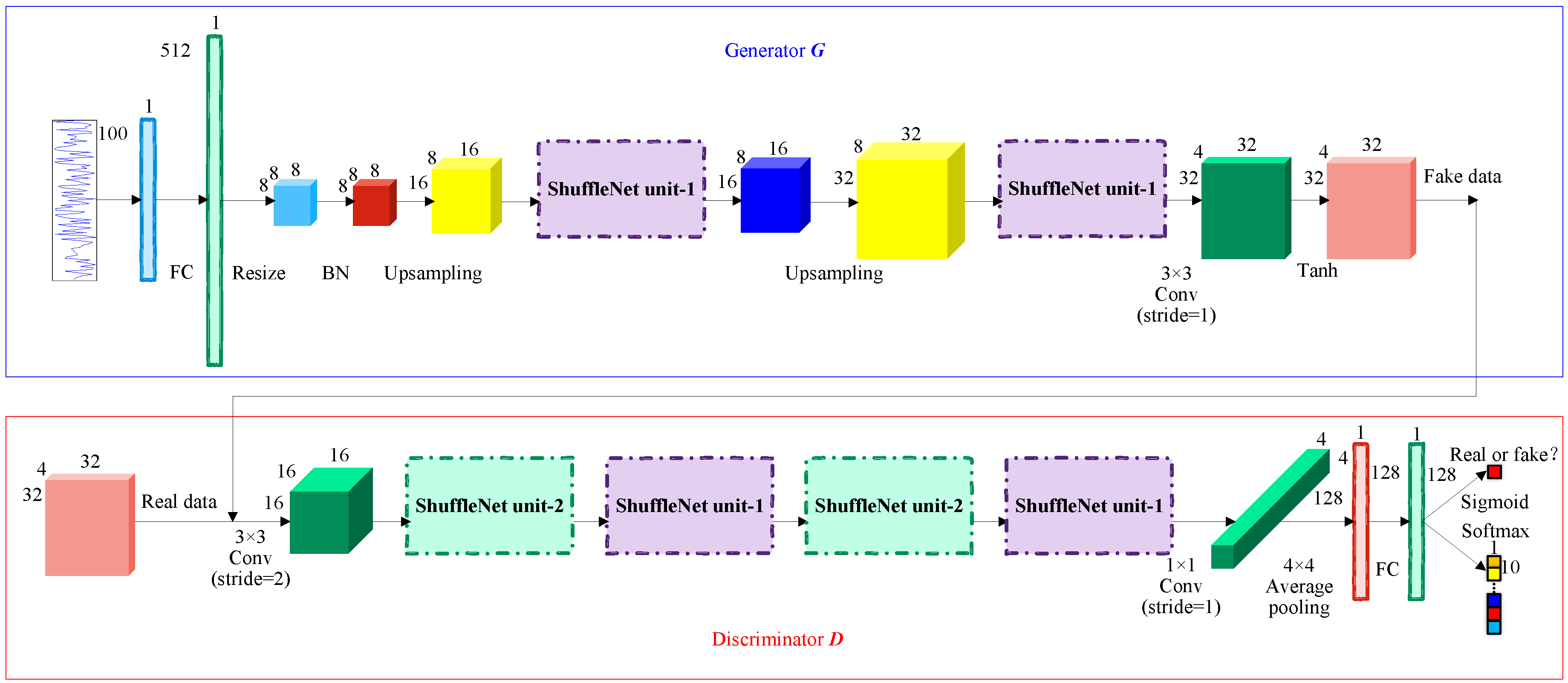
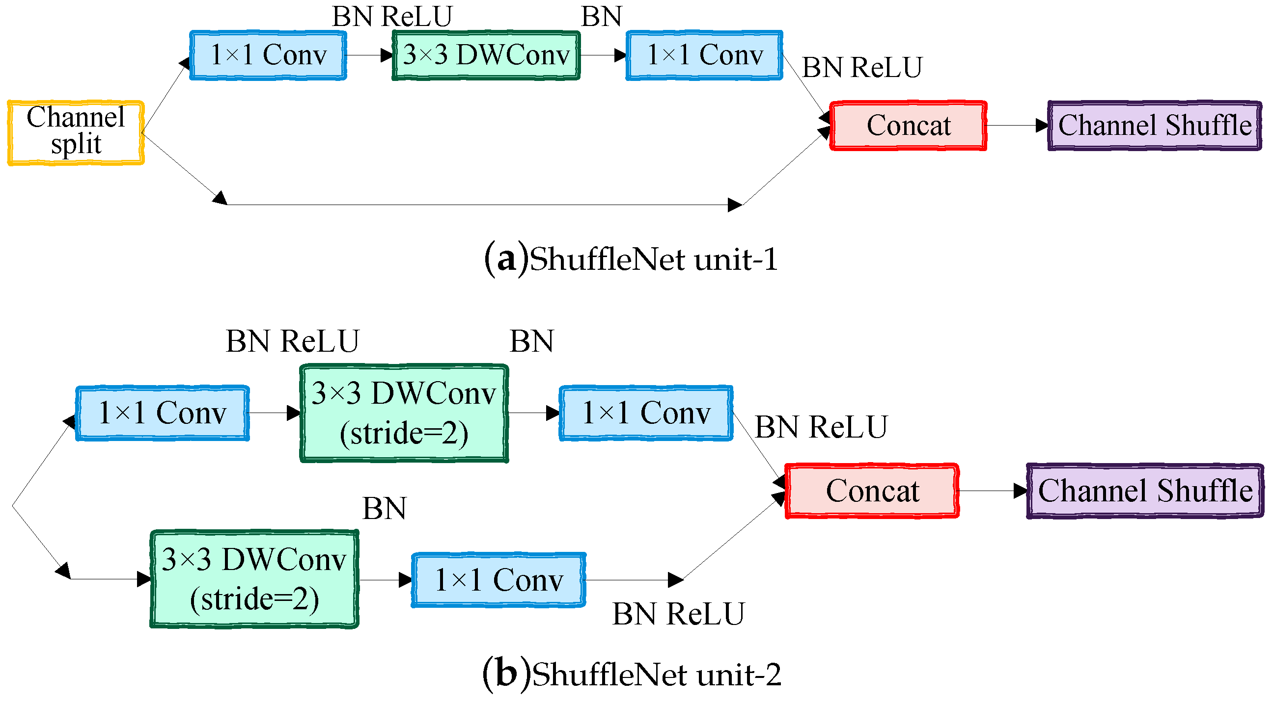
ShuffleGAN is proposed to extract high-level features for semi-supervised classification of wetland species with limited labeled samples. The architecture of the ShuffleGAN is depicted in Figure 3, which consists of two “adversarial” subnetworks: a generative model that generates a sample approximates the distribution of the training (real) data and a discriminative model that separates the fake and real samples as well as the class labels of real samples. Moreover, the ShuffleNet units (i.e., ShuffleNet unit-1 and ShuffleNet unit-2) used in and are shown in Figure 4.
In the generator , the input is the noise and the output is the fake data with desired size. FC is a fully connected layer, which takes the noise as input. FC is closely followed by resizing the layer, which resizes the output of FC into 3D cube. After the resize layer comes batch normalization (BN), which enables faster and more stable training of deep networks. Abstract features are then extracted by ShuffleNet unit-1, which greatly reduces the computation cost while maintaining accuracy. The upsampling layer is adopted to rescales the front layer to a larger size. Conv is the convolution layer, which extracts the features of the wetland data further. The Tanh activation function is used in the generator and the final output is a fake data, which is offered to the discriminator .
In the discriminator , the input is the real data from wetland image or the fake data generated by . The convolution layer (i.e., Conv) is used to extract the features of the input data, followed by several ShuffleNet unit-2 and ShuffleNet unit-1 blocks. ShuffleNet unit-1 is the basic unit while ShuffleNet unit-2 is the unit for spatial downsampling [34]. The structure of the ShuffleNet unit-1 is shown in Figure 4a. In the ShuffleNet unit-1, a channel split operator is performed to achieve high model capacity and efficiency by maintaining wide channels with neither dense Conv nor too many groups. By using the channel split operator, the inputs of the ShuffleNet unit-1 are split into two branches. One branch remains as identity and the other branch consists of two Conv layers and a depthwise convolution (i.e., DWConv) layer. The three convolutions have the same input and output channels. The two branches are then concatenated after convolution and a channel shuffle layer is used to communicate the information of the two branches. The structure of the ShuffleNet unit-2 is shown in Figure 4b. Compared with the ShuffleNet unit-1, the network structure of ShuffleNet unit-2 is slightly modified. We remove the channel split operator and directly perform two branches of feature extraction on the inputs. One branch contains three convolution layers (i.e., two Conv layers and a DWConv layer), while another branch consists of a DWConv layer and a Conv layer. Subsequently, the two branches are also concatenated and the channels are shuffled. The output channels of the ShuffleNet unit-2 is doubled. Following the ShuffleNet units comes another convolution layer, an average pooling layer and a FC layer. As for the last layer of the discriminator, a number of unlabeled samples are used in the training phase and is trained to distinguish the real data from fake data by using a sigmoid activation function, while the softmax function replaces the sigmoid function in the finetuning and classification phase so as to assign the input data to different classes.
After the architecture of the ShuffleGAN is constructed, we train the model for many epochs by using the limited labeled samples and lots of unlabeled samples. To address the instability of the ShuffleGAN, feature matching strategy is utilized to specify the objective of the generator , that means, is optimized by minimizing the following loss function
where and are the real data and fake data, respectively, denotes the feature extraction function by joining the Conv, Shuffle units, average pooling and FC in and is the expectation. Based on Equation (1), the generator is trained to match the expected value of the features on an intermediate layer of and thus, we can prevent from overtraining on the current discriminator.
On the other hand, the discriminator is optimized by minimizing the following loss function
where and are the real data and fake data generated by , respectively, is the probability distribution, C represents the class label and S denotes whether the input data of is “real” or “fake”. Moreover, Adamax method is used to obtain the optimal parameters of and .
3. Experiments and Analysis
3.1. Study Area and Dataset
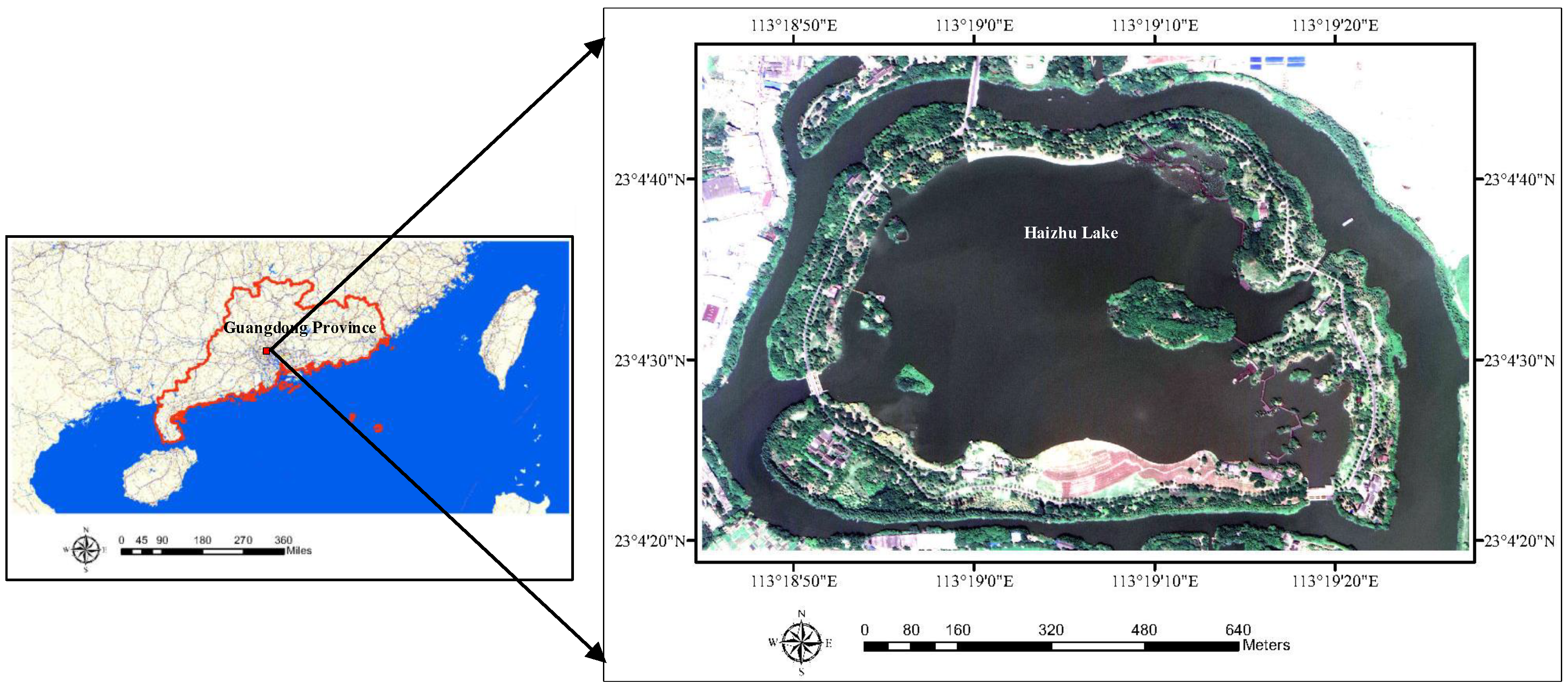
The study area (i.e., Haizhu Lake, see Figure 5) is chosen from the Haizhu wetland, which is located at the Haizhu district, Guangdong Province, China. Haizhu wetland plays an important role in regulating the climate, purifying the air and improving the urban ecological environment. It is also the largest national wetland park in the central of a megacity in China.
The remote sensing dataset was captured by the Jilin-1 satellite in 2017. This dataset consists of 4 spectral bands (i.e., blue, green, red and near-infrared) with a spatial resolution of 0.71 m per pixel. The spatial resolution of the Jilin-1 satellite image was further improved to 0.14 m by fusing with the google earth image gathered in 2017 [35]. Based on the above analysis, the study area has 4 spectral bands and the size of each band is .
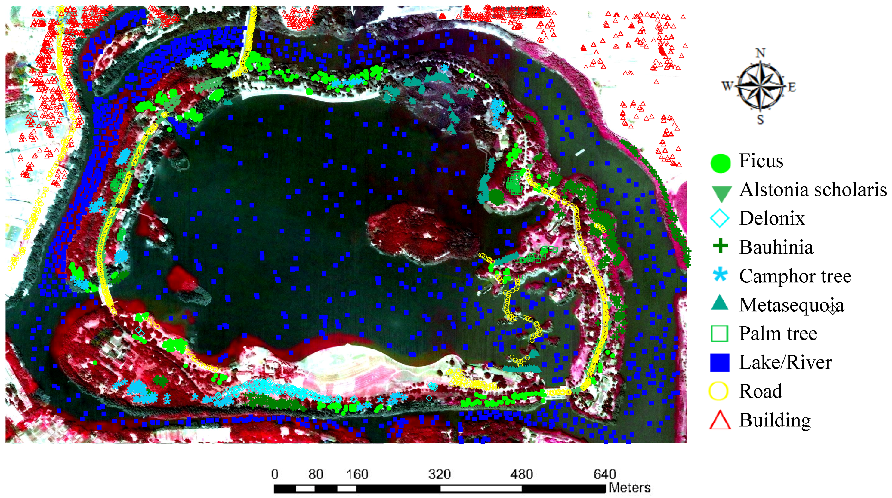
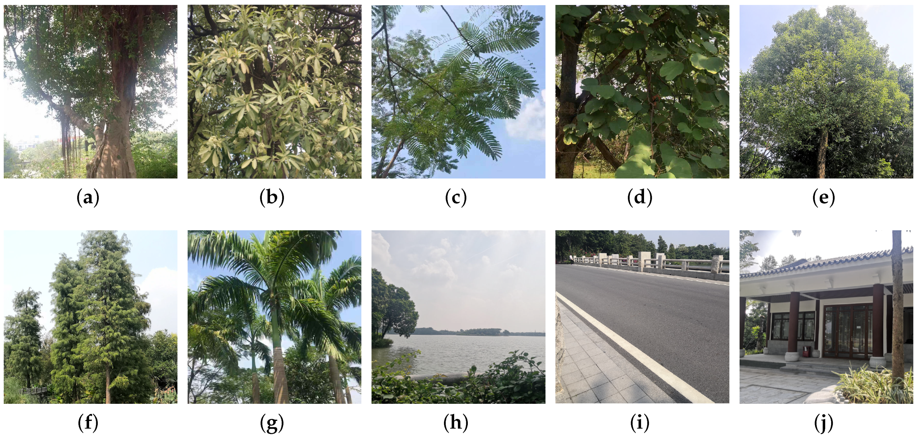
In-situ data for 10 classes of land-covers are collected for 675 points by recording Global Positioning System (GPS) points at each location. Subsequently, those points are used to manually label 4780 pixels on the dataset by remote sensing and expert biologists familiar with the Haizhu Lake. The classes and number of samples used in the experiments are displayed in Table 3, whose background color in the second column represents different classes of land-covers. Moreover, the color composite image with sampling sites is plotted in Figure 6 and the ground reference photos of different classes are shown in Figure 7.
3.2. Experimental Settings
The purpose of the experiments is to evaluate the effectiveness of the proposed ShuffleGAN for wetland classification. To that end, we compare ShuffleGAN with multiple state-of-the-art classification methods, including SVM, SVM with superpixel segmentation (abbreviated as SVM-s), LapSVM, LapSVM with superpixel segmentation (abbreviated as LapSVM-s), CNN, original GAN (abbreviated as GAN-or) and GAN with depthwise separable convolutions (GAN-dw). Details of the algorithms are described in the following:
- SVM: the classical SVM with radial basis function (RBF) kernel and using spectral features;
- SVM-s: the object-based SVM, whose objects are generated by SLIC and spectral-spatial features of each object are obtained by mean, standard deviation and entropy;
- LapSVM: the classical graph-based semi-supervised learning method using spectral features;
- LapSVM-s: the object-based LapSVM, whose objects are generated by SLIC and spectral-spatial features of each object are obtained by mean, standard deviation and entropy;
- CNN: the CNN classifier, which is made of Conv, BN, ReLU, pooling, FC and softmax layers;
- GAN-or: the original semi-supervised GAN, which does not contain Shufflenet units and depthwise separable convolutions;
- GAN-dw: the semi-supervised GAN, which uses depthwise separable convolutions.
Note that: (1) the above-mentioned SVM and LapSVM are pixel-based methods that only use spectral information, while the other ones are object-based methods applying spectral-spatial information; (2) the CNN, GAN-or, GAN-dw and ShuffleGAN are deep learning-based methods, while the others are based on SVM; and (3) the SVM, SVM-s and CNN are supervised methods, while the remaining ones are semi-supervised methods.
Several parameters should be tuned in the experiments. For the SVM-based methods (i.e., SVM, SVM-s, LapSVM and LapSVM-s), the RBF parameter is tuned in the range and the penalty term is selected in the range of 1 to 1000 with a step of 10. For the deep learning-based methods (i.e., CNN, GAN-or, GAN-dw and ShuffleGAN), the networks are configured as similar to each other as possible for fair comparison. The initial learning rate, patch size, batch size and training epochs are set to 0.001, 32, 128 and 200, respectively. The superpixel number is set to 4764 in the SLIC. Moreover, all available labeled samples are randomly divided into three parts, that is, about 10% for training, 5% for validation and 85% for testing (see Table 3). Notably that unlabeled samples can be adopted in the semi-supervised methods, about 2025 extra samples randomly chosen from the unlabeled sites are added for training. All the methods are quantitatively compared by three popular indexes, that is, overall accuracy (OA), average accuracy (AA) and kappa coefficient ().
3.3. Experimental Results
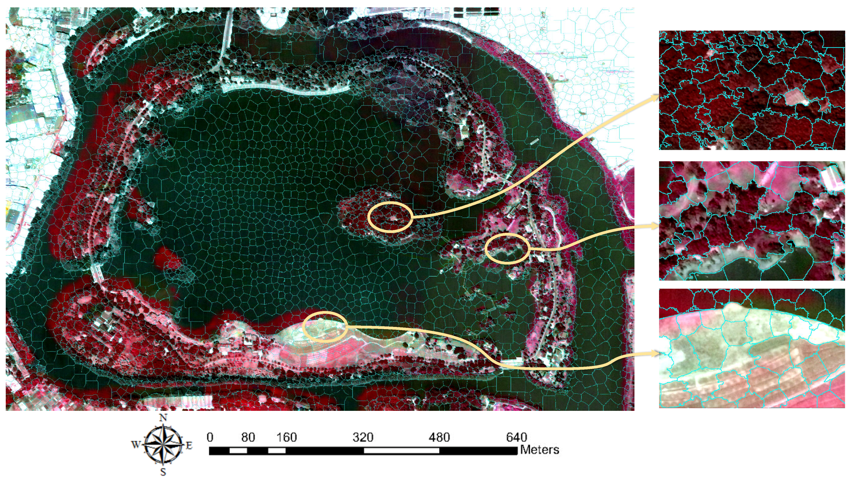
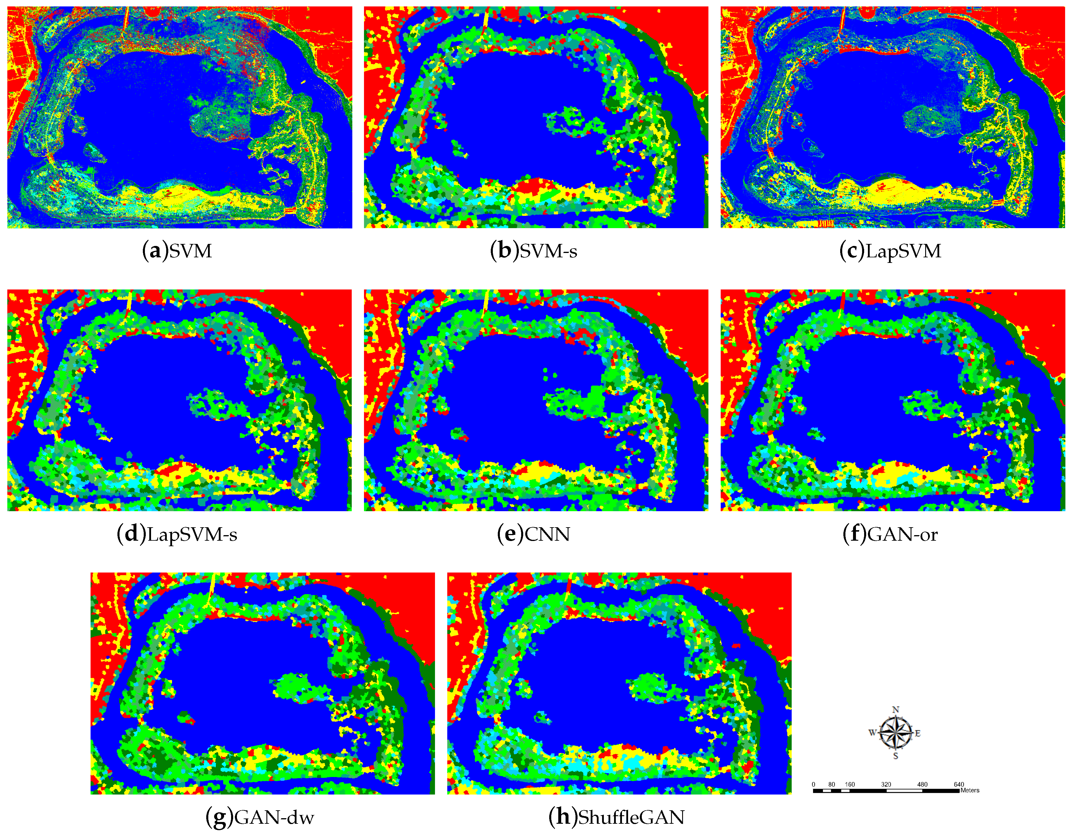
The superpixel segmentation results of the Haizhu Lake wetland data are shown in Figure 8, it is found that the experimental data is flexibly divided into naturally formed spatial areas with irregular sizes and shapes. The qualitative evaluations of different methods are listed in Table 4 and the classification maps are visually compared in Figure 9. Moreover, Figure 10 depicts the normalized confusion matrices for all of the methods. A few observations are noteworthy from the reported results. It can be first seen that the SVM and LapSVM, which are based only on spectral information, achieve lower classification performance than the results obtained by spectral-spatial features. As illustrated in Table 4, the SVM-s outperforms SVM by 7.38%, 12.03% and 9.14% in terms of OA, AA and , respectively. The OA of LapSVM-s is 68.93%, which is increased by 6.58% compared with that of LapSVM. Since the SVM and LapSVM utilize spectral features without any spatial prior, it is apparent that the spatial information can alleviate the spectral variations and stabilize the pixel-based features. Therefore, it is important to improve the wetland classification performance by jointly using the spectral-spatial information.
The semi-supervised methods are superior to or comparable with their supervised counterparts. As shown in Table 4, the LapSVM-s improves the OA, AA and of SVM-s by 1.93%, 3.58% and 2.38%, respectively. The GAN-or also increases 2.90%, 5.72% and 3.41% in OA, AA and compared with that of CNN. In addition, as displayed in Figure 9, the classification map of LapSVM-s (or GAN-or) is closer to the ground truth (see Figure 6) than SVM-s (or CNN). It is not hard to infer that the supervised methods using only the limited labeled samples generate worse classification results than the semi-supervised ones that take the unlabeled training samples into consideration. This stresses the importance of unlabeled samples for wetland classification.
Deep learning methods perform better than the SVM based methods. One can clearly see from Table 4 that the CNN/GAN-or/GAN-dw/ShuffleGAN significantly improve the classification accuracy of SVM/SVM-s/LapSVM/LapSVM-s. For instance, CNN outperforms SVM by 12.35%, 19.75% and 15.23% in terms of OA, AA and , respectively. This is due to the fact that deep learning methods can learn high-level representations of the input data and each layer of those methods extracts meaningful features from the lower layer and obtain much more abstract concepts than lower layers.
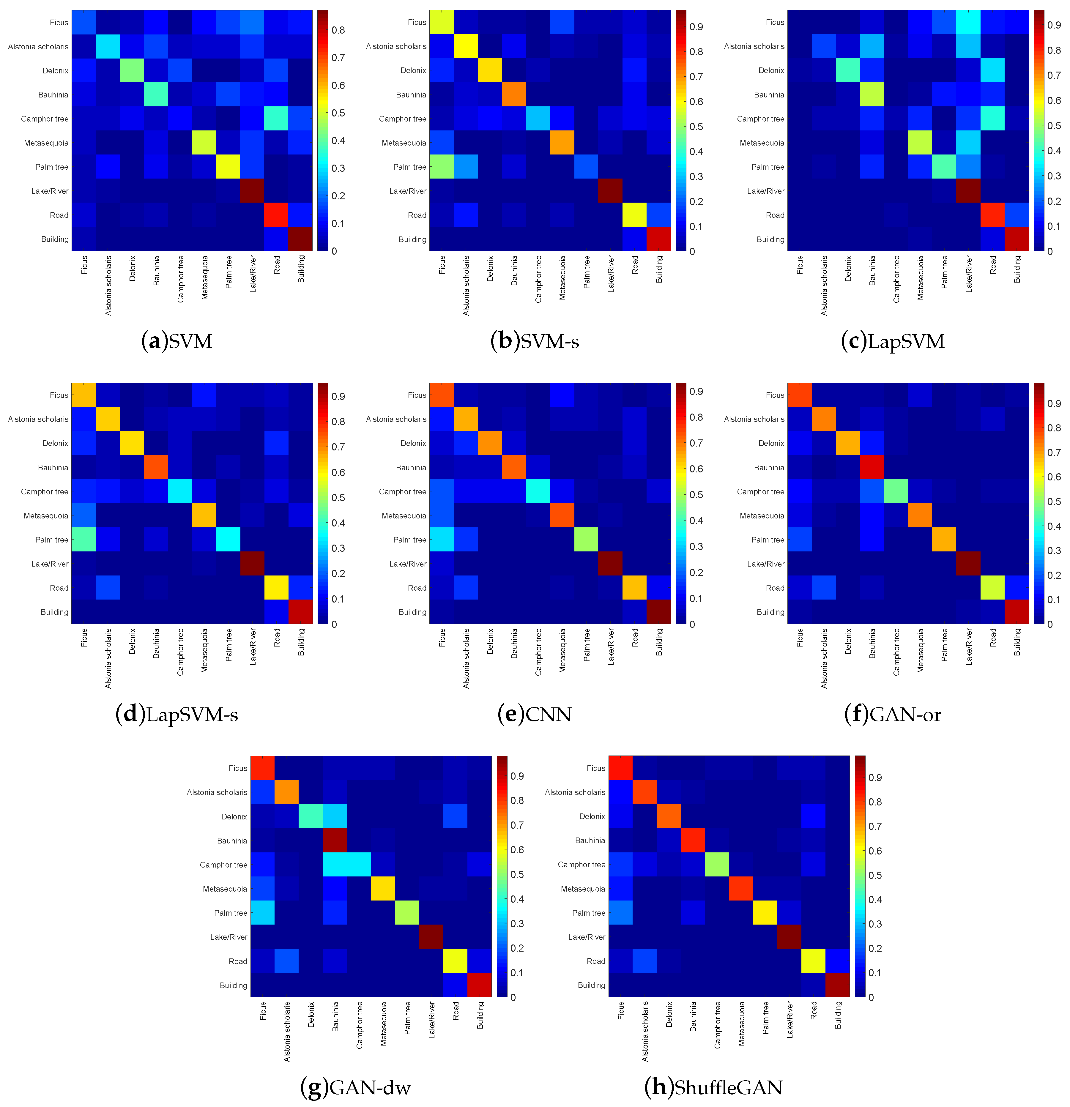
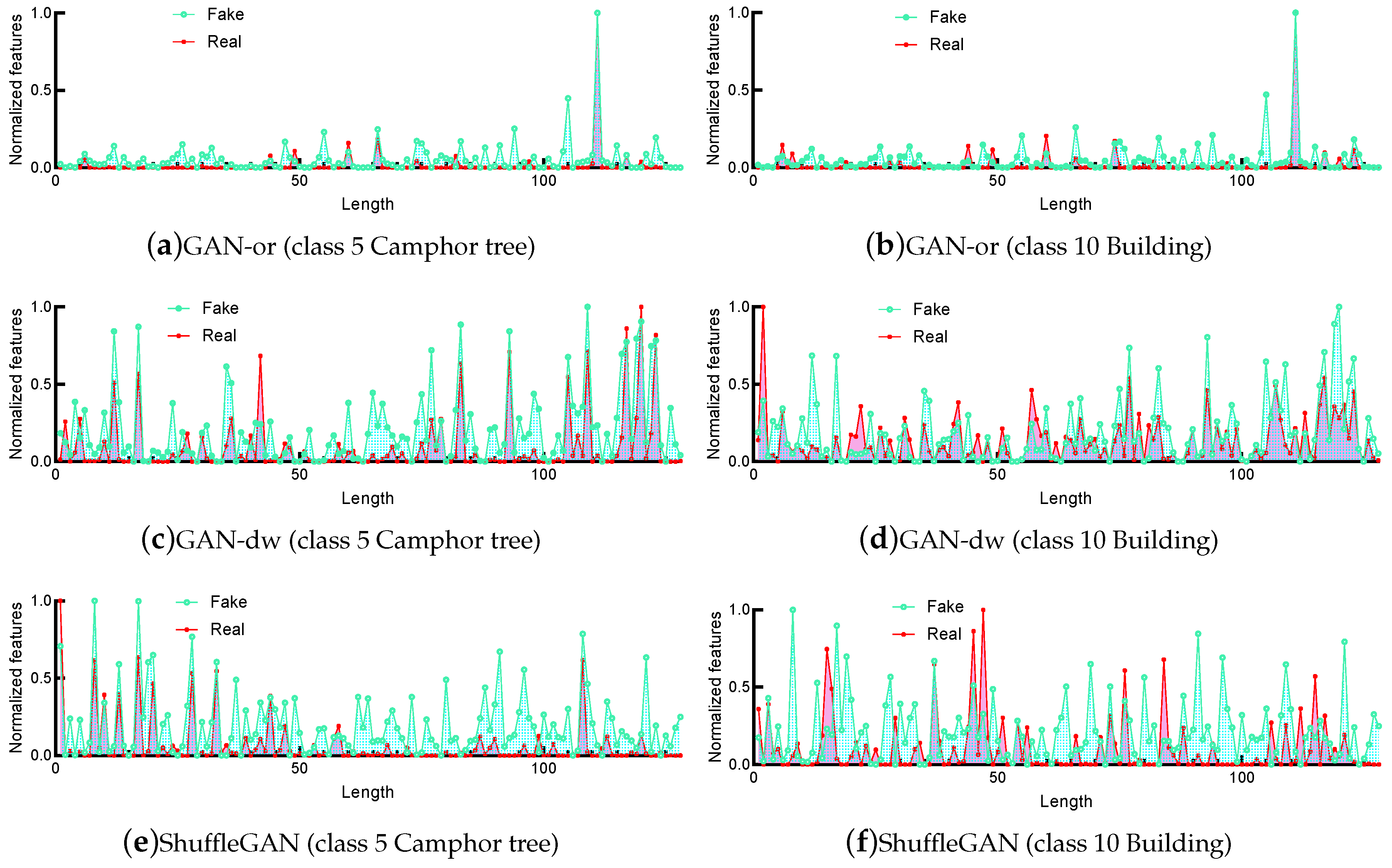
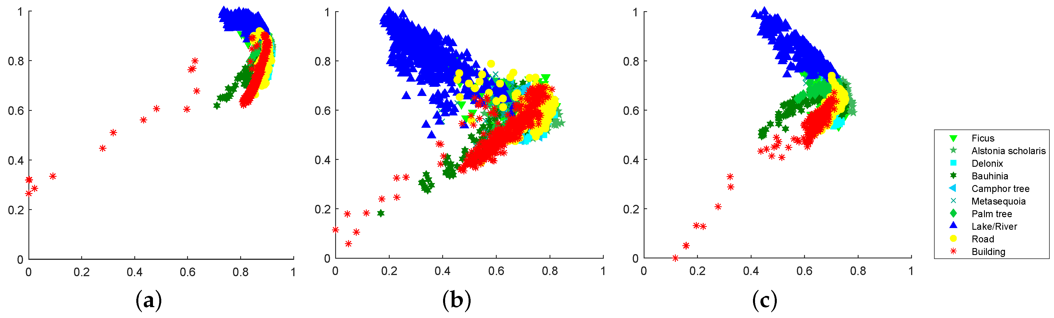
ShuffleGAN exhibits the best classification performance. From Table 4, one can see that for the Haizhu Lake wetland data, the ShuffleGAN achieves the highest OA, AA and , with an improvement of 2.10%, 2.73% and 2.45% over GAN-or, respectively. As shown in Figure 9, the classification map of ShuffleGAN has fewer misclassification errors than other methods. The normalized confusion matrices are compared in Figure 10. From Figure 10, all methods distinguish the non-wetland classes (i.e., classes 8 to 10) with producer’s accuracies exceeding 55%. The wetland classes (i.e., classes 1 to 7) are more difficult to separate than non-wetland ones. For instance, the producer’s accuracy of Camphor tree (i.e., class 5) obtained by LapSVM is as low as 4.46%, while the proposed ShuffleGAN classifies Camphor tree with producer’s accuracy up to 51.79%. The classes of Ficus and Alstonia scholaris (i.e., classes 1 and 2) are identified with accuracies beyond 80%. To provide intuitive insight, the normalized features of classes 5 and 10 obtained by GAN-or, GAN-dw and ShuffleGAN are compared in Figure 11, from which we can observe that the features of real data are more similar to those of the generated fake data obtained by ShuffleGAN. The scattering map of the two-dimensional features extracted by the discriminator of GAN-or, GAN-dw and ShuffleGAN are plotted in Figure 12, from which we can see that the representation learned by ShuffleGAN are more separable than the other methods. As such, it is easier to classify different features obtained by ShuffleGAN. Moreover, the computation time of ShuffleGAN is comparable with that of other methods. As displayed in Table 4, although the ShuffleGAN takes more time than SVM-based methods and GAN-dw, it is faster and more efficient than the CNN and GAN-or. In short, the experimental results demonstrate the effectiveness of the proposed ShuffleGAN in the classification of wetland data.
4. Discussions
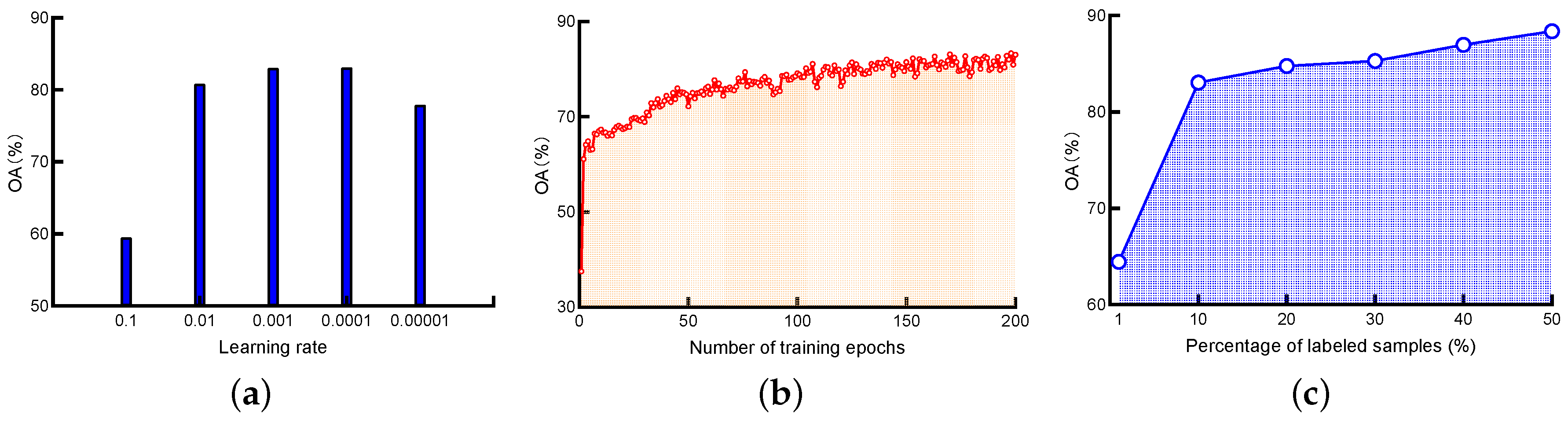
In this section, the influence of three important parameters, that is, initial learning rate, number of training epochs and number of labeled training samples on the performance of the ShuffleGAN is discussed. Figure 13 plots the OA of ShuffleGAN when the above-mentioned three parameters vary. The impact of initial learning rate is shown in Figure 13a, from which one can find that the OA with too large learning rate (e.g., 0.1) is lower than that with smaller ones. As an example, the OA is less than 60% in the case where the learning is set to 0.1, while the OA is higher than 70% if the learning rate is lower or equal to 0.01. The reason is that large learning rate will make the loss function to fluctuate around the minimum or even does not converge.
The OA against the number of training epochs is depicted in Figure 13b. The number of training epochs is varied within the range from 1 to 200. We can observe a dramatically upward tendency appeared with an initial increase of training epochs and then increases slowly and finally trends to stable. With this analysis in mind, it is better to train the network for more than 100 epochs to receive satisfactory classification results.
Finally, the impact of the number of labeled training samples is also evaluated in the experiments. We randomly choose 1%, 10%, 20%, 30%, 40% and 50% samples per class as labeled training samples and the OA of ShuffleGAN is shown in Figure 13c, which demonstrates that the classification accuracy increases as the number of labeled training samples goes up. The OA is consistently higher than 80% when the labeled samples are equal to or larger than 10%. Note that the OA of most competing methods is lower than 80% with 10% labeled samples, our proposed method is superior to other methods especially in the limited-labeled-sample scenario.
5. Conclusions
In this paper, we have proposed a new efficient deep network architecture, namely ShuffleGAN, for wetland species classification with limited labeled training samples. The underlying idea of ShuffleGAN is to explore the high-level abstract features of different species by an adversarial game between two neural networks. To that end, objects are constructed by superpixel segmentation, which is much more flexible than fixing the window size. ShuffleNet units are employed to obtain a good tradeoff between speed and accuracy in both generator and discriminator. ShuffleGAN is trained in a semi-supervised manner, which can make full use of both limited labeled samples and lots of unlabeled samples. The test samples can be fed into the trained network and classified by the discriminator. Experimental results on the Haizhu Lake wetland data demonstrate that the proposed ShuffleGAN method outperforms the state-of-the-art classifiers in terms of visual quality and classification accuracy. The computation time of ShuffleGAN is also acceptable, which is important for practical execution of the proposed method in real applications. As future work, we will try to adaptively decide the optimal network parameters. Moreover, it would be a great interest to use only unlabeled samples in the deep network for feature representation of various land-covers.
Author Contributions
All coauthors made significant contributions to the manuscript. Z.H. designed the research framework, analyzed the results and wrote the manuscript. D.H., X.M. and S.H. assisted in the prepared work and validation work. Moreover, all coauthors contributed to the editing and review of the manuscript.
Acknowledgments
This work was supported in part by the National Key R&D Program of China under Grant Nos. 2018YFB0505500 and 2018YFB0505503, the Fundamental Research Funds for the Central Universities under Grant No. 19lgzd10, the National Natural Science Foundation of China under Grant Nos. 41501368 and 41531178, the Young Teachers Development Foundation of City College of Dongguan University of Technology under Grant No. 2018QJY001Z and 2019 Special Funds for the Cultivation of Guangdong College Students’ Scientific and Technological Innovation “Climbing Program Special Funds” under Grant No. pdjh2019b0623. The authors would like to take this opportunity to thank the Editors and the Anonymous Reviewers for their detailed comments and suggestions, which greatly helped us to improve the clarity and presentation of our manuscript.
Conflicts of Interest
The authors declare no conflict of interest.
References
- Amani, M.; Mahdavi, S.; Afshar, M.; Brisco, B.; Huang, W.; Mohammad Javad Mirzadeh, S.; White, L.; Banks, S.; Montgomery, J.; Hopkinson, C. Canadian wetland inventory using google earth engine: The first map and preliminary results. Remote Sens. 2019, 11, 842. [Google Scholar] [CrossRef]
- Lane, C.; Liu, H.; Autrey, B.; Anenkhonov, O.; Chepinoga, V.; Wu, Q. Improved wetland classification using eight-band high resolution satellite imagery and a hybrid approach. Remote Sens. 2014, 6, 12187–12216. [Google Scholar] [CrossRef]
- Mleczko, M.; Mróz, M. Wetland mapping using sar data from the sentinel-1a and tandem-x missions: A comparative study in the biebrza floodplain (Poland). Remote Sens. 2018, 10, 78. [Google Scholar] [CrossRef]
- Mahdavi, S.; Salehi, B.; Granger, J.; Amani, M.; Brisco, B.; Huang, W. Remote sensing for wetland classification: A comprehensive review. GISci. Remote Sens. 2018, 55, 623–658. [Google Scholar] [CrossRef]
- Sánchez-Espinosa, A.; Schröder, C. Land use and land cover mapping in wetlands one step closer to the ground: Sentinel-2 versus landsat 8. J. Environ. Manag. 2019, 247, 484–498. [Google Scholar] [CrossRef]
- Zhao, J.; Yu, L.; Xu, Y.; Ren, H.; Huang, X.; Gong, P. Exploring the addition of Landsat 8 thermal band in land-cover mapping. Int. J. Remote Sens. 2019, 40, 4544–4559. [Google Scholar] [CrossRef]
- Zhu, X.; Hou, Y.; Weng, Q.; Chen, L. Integrating UAV optical imagery and LiDAR data for assessing the spatial relationship between mangrove and inundation across a subtropical estuarine wetland. ISPRS J. Photogramm. Remote Sens. 2019, 149, 146–156. [Google Scholar] [CrossRef]
- Araya-López, R.A.; Lopatin, J.; Fassnacht, F.E.; Hernández, H.J. Monitoring Andean high altitude wetlands in central Chile with seasonal optical data: A comparison between Worldview-2 and Sentinel-2 imagery. ISPRS J. Photogramm. Remote Sens. 2018, 145, 213–224. [Google Scholar] [CrossRef]
- Campbell, A.; Wang, Y. High spatial resolution remote sensing for salt marsh mapping and change analysis at fire island national seashore. Remote Sens. 2019, 11, 1107. [Google Scholar] [CrossRef]
- Wang, X.; Gao, X.; Zhang, Y.; Fei, X.; Chen, Z.; Wang, J.; Zhang, Y.; Lu, X.; Zhao, H. Land-Cover classification of coastal wetlands using the RF algorithm for Worldview-2 and Landsat 8 images. Remote Sens. 2019, 11, 1927. [Google Scholar] [CrossRef]
- Abeysinghe, T.; Simic Milas, A.; Arend, K.; Hohman, B.; Reil, P.; Gregory, A.; Vázquez-Ortega, A. Mapping invasive phragmites australis in the old woman creek estuary using UAV remote sensing and machine learning classifiers. Remote Sens. 2019, 11, 1380. [Google Scholar] [CrossRef]
- Cao, J.; Leng, W.; Liu, K.; Liu, L.; He, Z.; Zhu, Y. Object-based mangrove species classification using unmanned aerial vehicle hyperspectral images and digital surface models. Remote Sens. 2018, 10, 89. [Google Scholar] [CrossRef]
- Cao, J.; Liu, K.; Liu, L.; Zhu, Y.; Li, J.; He, Z. Identifying mangrove species using field close-range snapshot hyperspectral imaging and machine-learning techniques. Remote Sens. 2018, 10, 2047. [Google Scholar] [CrossRef]
- Ahmed, K.R.; Akter, S. Analysis of landcover change in southwest Bengal delta due to floods by NDVI, NDWI and K-means cluster with Landsat multi-spectral surface reflectance satellite data. Remote Sens. Appl. Soc. Environ. 2017, 8, 168–181. [Google Scholar] [CrossRef]
- Snedden, G.A. Patterning emergent marsh vegetation assemblages in coastal Louisiana, USA, with unsupervised artificial neural networks. Appl. Veg. Sci. 2019, 22, 213–229. [Google Scholar] [CrossRef]
- Sannigrahi, S.; Chakraborti, S.; Joshi, P.K.; Keesstra, S.; Sen, S.; Paul, S.K.; Kreuter, U.; Sutton, P.C.; Jha, S.; Dang, K.B. Ecosystem service value assessment of a natural reserve region for strengthening protection and conservation. J. Environ. Manag. 2019, 244, 208–227. [Google Scholar] [CrossRef] [PubMed]
- Hakdaoui, S.; Emran, A.; Pradhan, B.; Lee, C.W.; Fils, N.; Cesar, S. A collaborative change detection approach on multi-sensor spatial imagery for desert wetland monitoring after a flash flood in southern Morocco. Remote Sens. 2019, 11, 1042. [Google Scholar] [CrossRef]
- Kordelas, G.; Manakos, I.; Aragonés, D.; Díaz-Delgado, R.; Bustamante, J. Fast and automatic data-driven thresholding for inundation mapping with Sentinel-2 data. Remote Sens. 2018, 10, 910. [Google Scholar] [CrossRef]
- Belkin, M.; Niyogi, P.; Sindhwani, V. Manifold regularization: A geometric framework for learning from labeled and unlabeled examples. J. Mach. Learn. Res. 2006, 7, 2399–2434. [Google Scholar]
- Melacci, S.; Belkin, M. Laplacian support vector machines trained in the primal. J. Mach. Learn. Res. 2011, 12, 1149–1184. [Google Scholar]
- Maulik, U.; Chakraborty, D. Learning with transductive SVM for semisupervised pixel classification of remote sensing imagery. ISPRS J. Photogramm. Remote Sens. 2013, 77, 66–78. [Google Scholar] [CrossRef]
- Chen, Y.; Lin, Z.; Zhao, X.; Wang, G.; Gu, Y. Deep learning-based classification of hyperspectral data. IEEE J. Sel. Top. Appl. Earth Obs. Remote Sens. 2014, 7, 2094–2107. [Google Scholar] [CrossRef]
- Zhu, X.X.; Tuia, D.; Mou, L.; Xia, G.S.; Zhang, L.; Xu, F.; Fraundorfer, F. Deep learning in remote sensing: A comprehensive review and list of resources. IEEE Geosci. Remote Sens. Mag. 2017, 5, 8–36. [Google Scholar] [CrossRef]
- Rezaee, M.; Mahdianpari, M.; Zhang, Y.; Salehi, B. Deep convolutional neural network for complex wetland classification using optical remote sensing imagery. IEEE J. Sel. Top. Appl. Earth Observ. Remote Sens. 2018, 11, 3030–3039. [Google Scholar] [CrossRef]
- Mahdianpari, M.; Salehi, B.; Rezaee, M.; Mohammadimanesh, F.; Zhang, Y. Very deep convolutional neural networks for complex land cover mapping using multispectral remote sensing imagery. Remote Sens. 2018, 10, 1119. [Google Scholar] [CrossRef]
- Liu, T.; Abd-Elrahman, A. Deep convolutional neural network training enrichment using multi-view object-based analysis of Unmanned Aerial systems imagery for wetlands classification. ISPRS J. Photogramm. Remote Sens. 2018, 139, 154–170. [Google Scholar] [CrossRef]
- Mohammadimanesh, F.; Salehi, B.; Mahdianpari, M.; Gill, E.; Molinier, M. A new fully convolutional neural network for semantic segmentation of polarimetric SAR imagery in complex land cover ecosystem. ISPRS J. Photogramm. Remote Sens. 2019, 151, 223–236. [Google Scholar] [CrossRef]
- Chen, Y.; Zhao, X.; Jia, X. Spectral-spatial classification of hyperspectral data based on deep belief network. IEEE J. Sel. Top. Appl. Earth Observ. Remote Sens. 2015, 8, 2381–2392. [Google Scholar] [CrossRef]
- He, K.; Zhang, X.; Ren, S.; Sun, J. Deep residual learning for image recognition. In Proceedings of the IEEE Conference on Computer Vision and Pattern Recognition, Las Vegas, NV, USA, 26 June–1 July 2016; pp. 770–778. [Google Scholar]
- Souly, N.; Spampinato, C.; Shah, M. Semi supervised semantic segmentation using generative adversarial network. In Proceedings of the IEEE International Conference on Computer Vision, Venice, Italy, 22–29 October 2017; pp. 5688–5696. [Google Scholar]
- He, Z.; Liu, H.; Wang, Y.; Hu, J. Generative adversarial networks-based semi-supervised learning for hyperspectral image classification. Remote Sens. 2017, 9, 1042. [Google Scholar] [CrossRef]
- Chen, C.; Ma, Y.; Ren, G. A convolutional neural network with fletcher–reeves algorithm for hyperspectral image classification. Remote Sens. 2019, 11, 1325. [Google Scholar] [CrossRef]
- Achanta, R.; Shaji, A.; Smith, K.; Lucchi, A.; Fua, P.; Süsstrunk, S. SLIC superpixels compared to state-of-the-art superpixel methods. IEEE Trans. Pattern Anal. Mach. Intell. 2012, 34, 2274–2282. [Google Scholar] [CrossRef] [PubMed]
- Ma, N.; Zhang, X.; Zheng, H.T.; Sun, J. Shufflenet v2: Practical guidelines for efficient cnn architecture design. In Proceedings of the European Conference on Computer Vision (ECCV), Munich, Germany, 8–14 September 2018; pp. 116–131. [Google Scholar]
- Laben, C.A.; Brower, B.V. Process for Enhancing the Spatial Resolution of Multispectral Imagery Using Pan-Sharpening. U.S. Patent 6,011,875, 4 January 2000. [Google Scholar]
Figure 1.
General architecture of the proposed method.

Figure 2.
Schematic illustration of constructing the objects.

Figure 3.
Architecture of the proposed ShuffleGAN.

Figure 4.
ShuffleNet unit-1 and ShuffleNet unit-2 used in the ShuffleGAN.

Figure 5.
Geographic location of the study area.

Figure 6.
Three-band false color composite of the wetland data with sampling sites.

Figure 7.
Ground reference photos of different classes in the study area: (a) Ficus, (b) Alstonia scholaris, (c) Delonix, (d) Bauhinia, (e) Camphor tree, (f) Metasequoia, (g) Palm tree, (h) Lake/River, (i) Road and (j) Building.
Figure 7.
Ground reference photos of different classes in the study area: (a) Ficus, (b) Alstonia scholaris, (c) Delonix, (d) Bauhinia, (e) Camphor tree, (f) Metasequoia, (g) Palm tree, (h) Lake/River, (i) Road and (j) Building.

Figure 8.
Superpixel segmentation result.

Figure 9.
Classification maps of the Haizhu Lake wetland data obtained by (a) Support Vector Machine (SVM), (b) SVM-s, (c) LapSVM, (d) LapSVM-s, (e) Convolutional Neural Network (CNN), (f) GAN-or, (g) GAN-dw and (h) ShuffleGAN.
Figure 9.
Classification maps of the Haizhu Lake wetland data obtained by (a) Support Vector Machine (SVM), (b) SVM-s, (c) LapSVM, (d) LapSVM-s, (e) Convolutional Neural Network (CNN), (f) GAN-or, (g) GAN-dw and (h) ShuffleGAN.

Figure 10.
Normalized confusion matrices of (a) SVM, (b) SVM-s, (c) LapSVM, (d) LapSVM-s, (e) CNN, (f) GAN-or, (g) GAN-dw and (h) ShuffleGAN.
Figure 10.
Normalized confusion matrices of (a) SVM, (b) SVM-s, (c) LapSVM, (d) LapSVM-s, (e) CNN, (f) GAN-or, (g) GAN-dw and (h) ShuffleGAN.

Figure 11.
Normalized features of class 5 (Camphor tree) and class 10 (Building) in the real data and generated fake data obtained by various methods. (a,b) GAN-or, (c,d) GAN-dw and (e,f) ShuffleGAN.
Figure 11.
Normalized features of class 5 (Camphor tree) and class 10 (Building) in the real data and generated fake data obtained by various methods. (a,b) GAN-or, (c,d) GAN-dw and (e,f) ShuffleGAN.

Figure 12.
Scattering map of the two-dimensional features obtained by the discriminator of (a) GAN-or, (b) GAN-dw and (c) ShuffleGAN.
Figure 12.
Scattering map of the two-dimensional features obtained by the discriminator of (a) GAN-or, (b) GAN-dw and (c) ShuffleGAN.

Figure 13.
Impact of the (a) initial learning rate, (b) number of training epochs and (c) number of labeled training samples on the overall accuracy (OA).
Figure 13.
Impact of the (a) initial learning rate, (b) number of training epochs and (c) number of labeled training samples on the overall accuracy (OA).


Table 1.
Detailed architecture of the generator in ShuffleGAN.
| Layer | Output Size | Kernel Size | Stride | Output Channel |
|---|---|---|---|---|
| Input | 100 × 1 | – | – | 1 |
| FC | 512 × 1 | – | – | 1 |
| Resize | 8 × 8 | – | – | 8 |
| BN | 8 × 8 | – | – | 8 |
| Upsampling | 16 × 16 | – | – | 8 |
| ShuffleNet unit-1 | 16 × 16 | 3 × 3 | 1 | 8 |
| Upsampling | 32 × 32 | – | – | 8 |
| ShuffleNet unit-1 | 32 × 32 | 3 × 3 | 1 | 8 |
| Conv | 32 × 32 | 3 × 3 | 1 | 4 |
| Tanh | 32 × 32 | – | – | 4 |
Table 2.
Detailed architecture of the discriminator in ShuffleGAN.
| Layer | Output Size | Kernel Size | Stride | Output Channel |
|---|---|---|---|---|
| Input | 32 × 32 | – | – | 4 |
| Conv | 16 × 16 | 3 × 3 | 2 | 16 |
| ShuffleNet unit-2 | 8 × 8 | 3 × 3 | 2 | 32 |
| ShuffleNet unit-1 | 8 × 8 | 3 × 3 | 1 | 32 |
| ShuffleNet unit-2 | 4 × 4 | 3 × 3 | 2 | 64 |
| ShuffleNet unit-1 | 4 × 4 | 3 × 3 | 1 | 64 |
| Conv | 4 × 4 | 1 × 1 | 1 | 128 |
| Average pooling | 1 × 1 | 4 × 4 | – | 128 |
| FC | 1 × 1 | – | – | 128 |
| Sigmoid | 1 × 1 | – | – | 1 |
| Softmax | 1 × 1 | – | – | 10 |
Table 3.
Number of Samples (NoS) and training samples used in the experiments.
| Class | Name | NoS | Training | Validation | Test |
|---|---|---|---|---|---|
| 1 | Ficus | 417 | 42 | 25 | 350 |
| 2 | Alstonia scholaris | 138 | 14 | 9 | 115 |
| 3 | Delonix | 154 | 16 | 6 | 132 |
| 4 | Bauhinia | 484 | 49 | 24 | 411 |
| 5 | Camphor tree | 135 | 14 | 9 | 112 |
| 6 | Metasequoia | 431 | 44 | 11 | 376 |
| 7 | Palm tree | 260 | 26 | 4 | 230 |
| 8 | Lake/River | 1200 | 120 | 87 | 993 |
| 9 | Road | 833 | 84 | 31 | 718 |
| 10 | Building | 1403 | 141 | 36 | 226 |
| Total | 5455 | 550 | 242 | 4663 |
Table 4.
Classification accuracy (%) of various methods for the Haizhu Lake wetland data, bold values indicate the best result for a row.
Table 4.
Classification accuracy (%) of various methods for the Haizhu Lake wetland data, bold values indicate the best result for a row.
| Class | SVM | SVM-s | LapSVM | LapSVM-s | CNN | GAN-or | GAN-dw | ShuffleGAN |
|---|---|---|---|---|---|---|---|---|
| 1 | 17.43 | 56.00 | 0.86 | 64.57 | 73.14 | 78.57 | 81.43 | 83.43 |
| 2 | 28.70 | 59.13 | 17.39 | 63.48 | 65.22 | 73.04 | 71.30 | 80.00 |
| 3 | 43.18 | 62.12 | 40.91 | 62.12 | 67.42 | 68.94 | 41.67 | 76.52 |
| 4 | 37.71 | 71.05 | 53.77 | 75.67 | 71.53 | 88.32 | 93.67 | 82.24 |
| 5 | 10.71 | 29.46 | 4.46 | 33.93 | 35.71 | 47.32 | 34.82 | 51.79 |
| 6 | 49.47 | 69.41 | 53.19 | 64.63 | 73.94 | 72.34 | 63.30 | 80.59 |
| 7 | 52.61 | 18.26 | 42.61 | 35.22 | 49.13 | 68.26 | 53.04 | 62.17 |
| 8 | 86.40 | 96.68 | 95.87 | 95.27 | 92.45 | 98.29 | 97.99 | 98.79 |
| 9 | 74.79 | 58.08 | 80.08 | 60.72 | 63.79 | 55.57 | 58.77 | 60.17 |
| 10 | 87.03 | 88.09 | 88.58 | 88.50 | 93.15 | 92.01 | 89.40 | 94.29 |
| OA | 66.20 | 73.58 | 68.93 | 75.51 | 78.55 | 81.45 | 79.28 | 83.55 |
| AA | 48.80 | 60.83 | 47.77 | 64.41 | 68.55 | 74.27 | 68.54 | 77.00 |
| 59.31 | 68.45 | 62.14 | 70.83 | 74.54 | 77.95 | 75.35 | 80.40 | |
| time(s) | 1.03 | 2.97 | 3.54 | 4.86 | 752.14 | 818.41 | 684.55 | 717.45 |
© 2019 by the authors. Licensee MDPI, Basel, Switzerland. This article is an open access article distributed under the terms and conditions of the Creative Commons Attribution (CC BY) license (http://creativecommons.org/licenses/by/4.0/).
Share and Cite
MDPI and ACS Style
He, Z.; He, D.; Mei, X.; Hu, S. Wetland Classification Based on a New Efficient Generative Adversarial Network and Jilin-1 Satellite Image. Remote Sens. 2019, 11, 2455. https://0-doi-org.brum.beds.ac.uk/10.3390/rs11202455
AMA Style
He Z, He D, Mei X, Hu S. Wetland Classification Based on a New Efficient Generative Adversarial Network and Jilin-1 Satellite Image. Remote Sensing. 2019; 11(20):2455. https://0-doi-org.brum.beds.ac.uk/10.3390/rs11202455
Chicago/Turabian StyleHe, Zhi, Dan He, Xiangqin Mei, and Saihan Hu. 2019. "Wetland Classification Based on a New Efficient Generative Adversarial Network and Jilin-1 Satellite Image" Remote Sensing 11, no. 20: 2455. https://0-doi-org.brum.beds.ac.uk/10.3390/rs11202455
Note that from the first issue of 2016, this journal uses article numbers instead of page numbers. See further details here.