Article

Retrieval of the Fraction of Radiation Absorbed by Photosynthetic Components (FAPARgreen) for Forest Using a Triple-Source Leaf-Wood-Soil Layer Approach

1
State Key Laboratory of Remote Sensing Science, Institute of Remote Sensing and Digital Earth, Chinese Academy of Sciences, Beijing 100094, China
2
College of Geomatics, Xi’an University of Science and Technology, Xi’an 710054, China
3
College of Resources and Environment, University of Chinese Academy of Sciences, Beijing 100049, China
4
State Key Laboratory of Remote Sensing Science, Beijing Key Laboratory of Environmental Remote Sensing and Digital City, School of Geography, Beijing Normal University, Beijing 100875, China
*
Author to whom correspondence should be addressed.
Remote Sens. 2019, 11(21), 2471; https://0-doi-org.brum.beds.ac.uk/10.3390/rs11212471
Submission received: 12 September 2019 / Revised: 10 October 2019 / Accepted: 18 October 2019 / Published: 23 October 2019
(This article belongs to the Special Issue Remote Sensing of Biophysical Parameters)

Abstract

:
The fraction of absorbed photosynthetically active radiation (FAPAR) is generally divided into the fraction of radiation absorbed by the photosynthetic components ( F A P A R g r e e n ) and the fraction of radiation absorbed by the non-photosynthetic components ( F A P A R w o o d y ) of the vegetation. However, most global FAPAR datasets do not take account of the woody components when considering the canopy radiation transfer. The objective of this study was to develop a generic algorithm for partitioning F A P A R c a n o p y into F A P A R g r e e n and F A P A R w o o d y based on a triple-source leaf-wood-soil layer (TriLay) approach. The LargE-Scale remote sensing data and image simulation framework (LESS) model was used to validate the TriLay approach. The results showed that the TriLay F A P A R g r e e n had higher retrieval accuracy, as well as a significantly lower bias (R2 = 0.937, Root Mean Square Error (RMSE) = 0.064, and bias = −6.02% for black-sky conditions; R2 = 0.997, RMSE = 0.025 and bias = −4.04% for white-sky conditions) compared to the traditional linear method (R2 = 0.979, RMSE = 0.114, and bias = −18.04% for black-sky conditions; R2 = 0.996, RMSE = 0.106 and bias = −16.93% for white-sky conditions). For FAPAR that did not take account of woody components ( F A P A R n o W A I ), the corresponding results were R2 = 0.920, RMSE = 0.071, and bias = −7.14% for black-sky conditions, and R2 = 0.999, RMSE = 0.043, and bias = −6.41% for white-sky conditions. Finally, the dynamic F A P A R g r e e n , F A P A R w o o d y , F A P A R c a n o p y and F A P A R n o W A I products for a North America region were generated at a resolution of 500 m for every eight days in 2017. A comparison of the results for F A P A R g r e e n against those for F A P A R n o W A I and F A P A R c a n o p y showed that the discrepancy between F A P A R g r e e n and other FAPAR products for forest vegetation types could not be ignored. For deciduous needleleaf forest, in particular, the black-sky F A P A R g r e e n was found to contribute only about 23.86% and 35.75% of F A P A R c a n o p y at the beginning and end of the year (from January to March and October to December, JFM and OND), and 75.02% at the peak growth stage (from July to September, JAS); the black-sky F A P A R n o W A I was found to be overestimated by 38.30% and 28.46% during the early (JFM) and late (OND) part of the year, respectively. Therefore, the TriLay approach performed well in separating F A P A R g r e e n from F A P A R c a n o p y , which is of great importance for a better understanding of the energy exchange within the canopy.

Graphical Abstract

1. Introduction

The fraction of absorbed photosynthetically active radiation (FAPAR) is a significant biochemical and physiological variable used in tracing the exchanges of energy, mass, and momentum, and is also widely used in many climate, ecological, biogeochemical, agricultural, and hydrology models [1,2]. FAPAR is, therefore, an important input parameter and widely used in satellite-based Production Efficiency Models (PEMs) [3,4,5,6] to estimate gross primary productivity (GPP) or net primary production (NPP).
In general, the FAPAR inversion algorithms could be divided into two types: empirical statistical models based on vegetation indexes and physical methods based on the canopy radiation transfer model. Although the empirical statistical model based on vegetation indexes is relatively simple, involves only a few parameters and has high computational efficiency, it is subject to many uncertainties due to factors such as the atmospheric environment, vegetation type, and quality of remote sensing data. The physically based methods could be further divided into two categories. The first type is the direct inversion method, which uses the canopy radiation transfer model to link FAPAR with the canopy spectra [7,8,9]. For example, the Moderate Resolution Imaging Spectroradiometer (MODIS) algorithm uses the three-dimensional radiation transmission model to invert FAPAR from the bi-directional reflectance [10,11,12]. The Joint Research Centre (JRC) FAPAR algorithm is also based on a physical model that uses a continuous vegetation canopy model [13] to link land surface reflectance with FAPAR. However, these methods are mostly based on the radiative transfer model; thus, the inversion process is complicated for retrieval of FAPAR. The main problem with such methods is that it is difficult to overcome the uncertainty caused by model coupling and spatial heterogeneity. The second type of physically based method is the forward modeling method [14,15,16,17,18,19]. Most models of this type are based on the gap fraction model, which determines FAPAR according to canopy structure parameters such as LAI and the clumping index. The disadvantage of this approach is that it relies too much on the accuracy of the canopy structure parameters. Furthermore, it is difficult to accurately determine the soil albedo and extinction coefficient, which are also important parameters needed to determine the contribution of multiple scattering between the soil and canopy to FAPAR [17].
Recently, several global FAPAR products have become available, including the Moderate Resolution Imaging Spectroradiometer (MODIS) [20,21], Energy Balance Residual (EBR) [15], Multi-angle Imaging SpectroRadiometer (MISR) [11], CYCLOPES [22], GLOBCARBON [23], Global Land Surface Satellite (GLASS) [14], the Medium Resolution Imaging Spectrometer (MERIS) [24], Joint Research Center Two Stream Inversion Package (JRC-TIP) [25], and European Space Agency (ESA) products [26]. These global FAPAR products have been widely validated, with reported errors varying from 0.08 to 0.23 [14,27,28,29,30,31,32]. However, most of the global FAPAR products do not consider the effect of non-photosynthetic components in the radiative transfer process, which introduces errors, especially for forest types. Moreover, many researchers have used the fraction of radiation absorbed by photosynthetic components ( F A P A R g r e e n ) instead of the fraction of radiation absorbed by the canopy ( F A P A R c a n o p y ) to monitor and estimate the light use efficiency (LUE), radiation use efficiency (RUE), and productivity at different temporal scales [33,34,35,36].
The forest vegetation ecosystem plays an important role in the global ecosystem. However, quantifying the temporal variation in F A P A R g r e e n for a forest ecosystem represents an important challenge for remote sensing and ecology researchers as it is extremely difficult to measure F A P A R g r e e n at large scales over plant growing seasons directly. Also, previous studies have shown that the contribution of woody components is relatively large: for instance, Asner et al. [37] found that stems increased F A P A R c a n o p y by 10–40%. Therefore, the partitioning of absorbed radiation into photosynthetic and non-photosynthetic parts is very important for better modeling of vegetation photosynthesis and energy exchange within the canopy.
Already, some studies have looked at the estimation of F A P A R g r e e n from remote sensing data. Hall et al. [38] estimated F A P A R g r e e n using a simple linear relationship between F A P A R c a n o p y and L A I g r e e n / L A I t o t a l ( L A I t o t a l denotes the total leaf area index including green and senescent leaves, while L A I g r e e n represents the green leaf area index). However, this simple partitioning is problematic because the green and woody components within the canopy do not constitute a simple linear mix in terms of radiation transfer. Zhang et al. [39] first retrieved the biophysical and biochemical variables using the modified PROSPECT model coupled with the SAIL-2 model (hereafter called PROSAIL-2 model), and then calculated F A P A R g r e e n and F A P A R c a n o p y using the forward simulation approach. However, F A P A R g r e e n retrieval using the PROSAIL-2 model is relatively complex and needs several physiological and biochemical parameters as model inputs. Gitelson et al. [40] also separated F A P A R c a n o p y into photosynthetically active green components ( F A P A R g r e e n ) and non-photosynthetic active components using the ratio L A I g r e e n / L A I t o t a l for maize and soybeans. The relationship between vegetation indices and F A P A R g r e e n was also used to retrieve F A P A R g r e e n [41,42]. Nevertheless, to date, the current F A P A R g r e e n products do not take into account the effect of non-photosynthetic components on canopy radiative transfer.
In this study, we aim to develop an operational algorithm for partitioning F A P A R c a n o p y into F A P A R g r e e n and F A P A R w o o d y for forest types. A simple triple-source leaf–wood–soil layer model (TriLay) that describes the radiation transfer within the canopy-soil system is presented. F A P A R c a n o p y is first separated into the fraction of PAR absorbed by the canopy for downwelling radiation ( F A P A R c a n o p y ) and the fraction of PAR absorbed by the canopy for the upwelling radiation reflected by the soil background ( F A P A R c a n o p y ). Then, F A P A R c a n o p y and F A P A R c a n o p y are further split into the fraction of radiation absorbed by photosynthetic components ( F A P A R g r e e n ) and that absorbed by non-photosynthetic components ( F A P A R w o o d y ) using the TriLay model. Finally, the F A P A R g r e e n , F A P A R w o o d y , and F A P A R c a n o p y products are generated using the MODIS albedo (MCD43A3), LAI (MCD15A2H), land cover (MCD12Q1), clumping index (CI), and soil albedo products based on the TriLay approach, and the discrepancies between different FAPAR products are used to investigate the contributions of woody components to the canopy-absorbed radiation. The partitioning of absorbed radiation into green and woody parts using the TriLay model is done not just to provide F A P A R g r e e n and F A P A R w o o d y —which is of great importance for better understanding the energy exchange within the canopy. The consideration of woody components should also improve the accuracy of F A P A R g r e e n estimates, which is important for better modeling of vegetation photosynthesis.

2. Materials and Methods

2.1. Satellite Datasets

In order to produce F A P A R g r e e n products, several satellite datasets were utilized in this study, including MODIS LAI products, land cover products, CI products, and soil albedo products from 2017. Data simulated by the LESS model [43] was used to validate the retrieved F A P A R g r e e n products. A mid-latitude region (tile h10v05, covering 30.00° N–40.00° N and 80.00° W–104.43° W) was selected to investigate the discrepancy between F A P A R g r e e n and other FAPAR products because there were abundant forest vegetation types within this MODIS tile.

2.1.1. MODIS LAI/FAPAR Products (MCD15A2H)

MCD15A2H V006 is a MODIS eight-day composite LAI/FAPAR product that includes FAPAR, LAI, and quality control (QC) data with a resolution of 500 m [44]. The main retrieval algorithm for LAI and FAPAR contains a Look-up-Table (LUT) based on a 3D radiation transfer model [21] that uses the atmospherically corrected Red and near-infrared (NIR) Bidirectional Reflectance Function (BRF) [45]. A back-up algorithm based on the empirical relationships between the Normalized Difference Vegetation Index (NDVI) and LAI and FAPAR at the canopy scale is used at the same time. Also, for the biome types and typical conditions that are considered, observed, and modeled spectral BRFs and soil patterns are compared for each pixel. The LAI and FAPAR values that lie within a fixed level of uncertainty are then taken to be acceptable. Finally, averaged values of LAI and FAPAR are used as the eventually retrieved values [20].

2.1.2. MODIS Land Cover Product (MCD12Q1)

The MODIS Land Cover Type Product (MCD12Q1) provides land cover maps with a temporal resolution of one year and a spatial resolution of 500m at a global scale from 2001 until the present; it includes several classification schemes (International Geosphere-Biosphere Programme (IGBP), University of Maryland (UMD), LAI, BIOME-Biogeochemical Cycles (DBC), Plant Functional Types (PFT), FAO-Land Cover Classification System land cover (LCCS1), etc.). The main algorithm used in MCD12Q1 is a supervised classification method (decision tree) combined with a boosting technique [20] based on MODIS reflectance data [46,47]. The International Geosphere-Biosphere Program (IGBP) classification scheme, which defines 17 land cover types, was used in this study.

2.1.3. Global Clumping Index (CI) Product

The clumping index (CI) signifies the characteristics of groups of foliage in the canopy, and thus, it is a significant parameter describing the structure of the vegetation canopy [48]. According to Jiao et al. [49], a method based on the MODIS Bidirectional Reflectance Distribution Function (BRDF) and a linear relationship between the CI and the normalized difference between the angular indexes of the hotspot and dark spot (NDHD) could be utilized to generate CIs within a valid range (0.33 to 1.00); a back-up algorithm is also used to substitute values for the invalid CIs [49]. A global CI dataset with an eight-day temporal resolution and 500 m spatial resolution covering the period from 2002 to the present has been produced by Jiao et al. [49].

2.1.4. Global Soil Albedo Product

A non-linear spectral mixture model (NSM) model proposed by Liu & Zhang (2018) [15,50] was used to retrieve the global visible (VIS) soil albedo. The main idea in the NSM model is the dual-source vegetation–soil layer approach. In this approach, it is assumed that the leaves are located in the upper canopy, while the soil components are found in the lower canopy. Based on this assumption, the canopy albedo can be approximated as a non-linear mixture of the “pure” vegetation and soil parts [15]. For pixels with abnormal values (smaller than 0.02 or greater than 0.3), prior values acquired by a global database of land surface parameters at 1 km resolution (ECOCLIMAP) [51,52] and the yearly composite value were used instead. Finally, the estimated global VIS soil albedo based on the NSM model is obtained, having a spatial resolution of 500 m and a temporal resolution of eight days.

2.2. Data Simulated by the LESS Model

To quantitatively evaluate the performance of the proposed TriLay approach for estimating F A P A R g r e e n , the LargE-Scale remote sensing data and image simulation (LESS) framework model [43] was employed to generate a simulated dataset that covered most of the conditions found in forests. LESS is a ray-tracing based 3D radiative transfer model which can simulate remote sensing data and images over large-scale and realistic 3D scenes (http://lessrt.org/). LESS employs a weighted forward photon tracing (FPT) method to simulate multispectral bidirectional reflectance factor (BRF) or flux-related data (e.g., downwelling radiation) and a backward path tracing (BPT) method to generate sensor images (e.g., fisheye images) or large-scale (e.g., 1 km2) spectral images. The accuracy of LESS is evaluated with other models as well as field measurements in terms of directional BRFs and pixel-wise simulated image comparisons, which shows very good agreement [43,53].
The modeling area is located in the Genhe Forestry Reserve (Genhe) (120 ° 12′ to 122 ° 55′ E, 50 ° 20′ to 52 ° 30′ N), Greater Khingan of Inner Mongolia, Northeastern China. It has a hilly terrain with 75% forest cover, which is mainly composed of Dahurian Larch (Larix gmelinii) and White Birch (Betula platyphylla Suk.). A pure plot of Dahurian Larch (L9) is established and is selected for modeling, with its location in Figure 1. The position, crown width, breast diameter, tree height, and transmittance for trees were entered into the LESS model. A total of eight scenes were constructed, with each individual tree in a scene consisting of branches and leaves. The branches and size of the woody area were kept the same in all the scenes, but the leaf area was changed to produce scenes with different values of the LAI. For each scene, different FAPAR values (including F A P A R c a n o p y , F A P A R g r e e n and F A P A R w o o d y ) were calculated under black-sky (the ratio of diffuse light is zero, and nine different solar zenith angles of 0°–80° at 10° intervals were set) and white-sky conditions (the ratio of diffuse light is 1). The main input parameters used in the LargE-Scale remote sensing data and image simulation (LESS) model are listed as Table 1. Finally, a total of 72 black-sky simulations and eight white-sky simulations were achieved for the different conditions giving.

2.3. Algorithms for Estimating Global F A P A R g r e e n and F A P A R w o o d y Datasets

To split the fraction of radiation absorbed by photosynthetic components ( F A P A R g r e e n ) from F A P A R c a n o p y , a novel triple-source leaf–wood–soil layer model was proposed for generating global F A P A R g r e e n products for forest vegetation types. Figure 2 is a flowchart of the process used to retrieve global F A P A R g r e e n products.
First, F A P A R c a n o p y is split into two parts: the fraction of PAR absorbed by the canopy for the downwelling radiation ( F A P A R c a n o p y ) and that absorbed by the canopy for the upwelling radiation reflected by the soil background ( F A P A R c a n o p y ). Then, F A P A R c a n o p y and F A P A R c a n o p y are further split into the fraction of radiation absorbed by photosynthetic components ( F A P A R g r e e n ) and that absorbed by non-photosynthetic components (e.g., branches and stems, hereafter called F A P A R w o o d y ). Finally, F A P A R g r e e n and F A P A R w o o d y can be calculated separately using the TriLay approach.

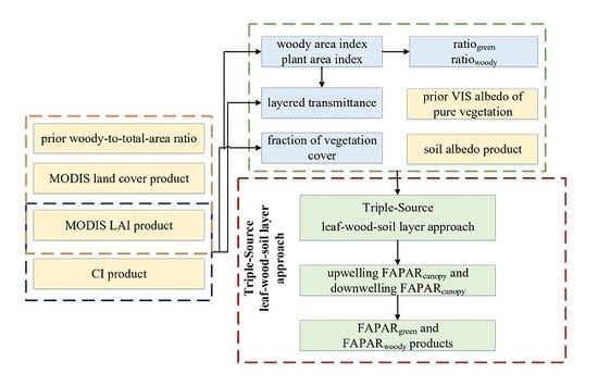
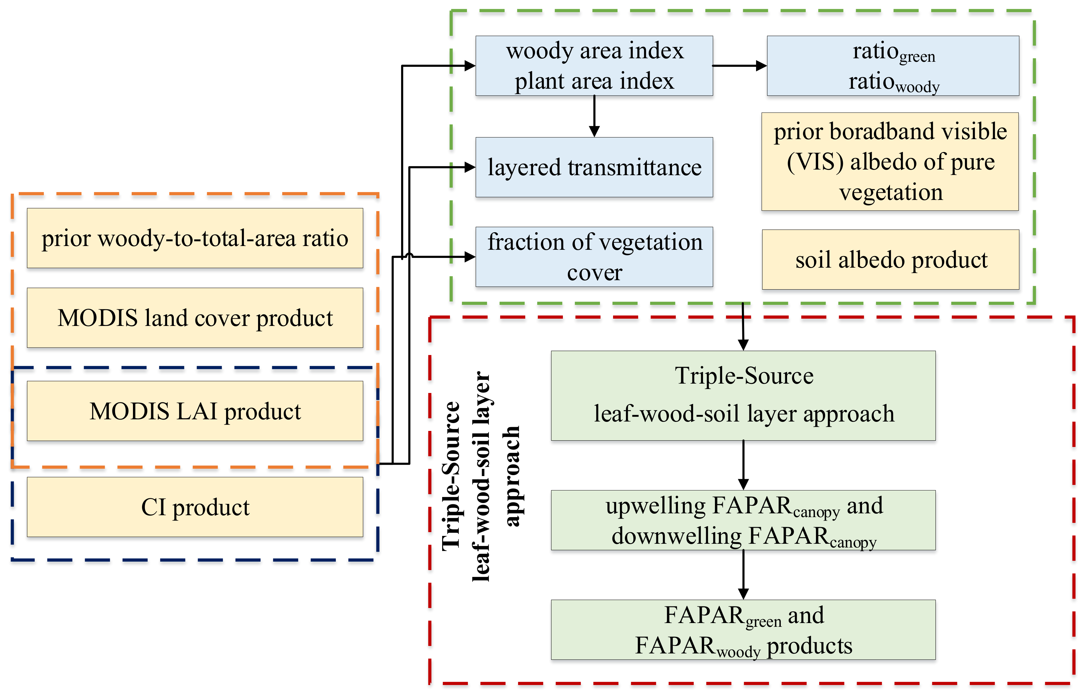
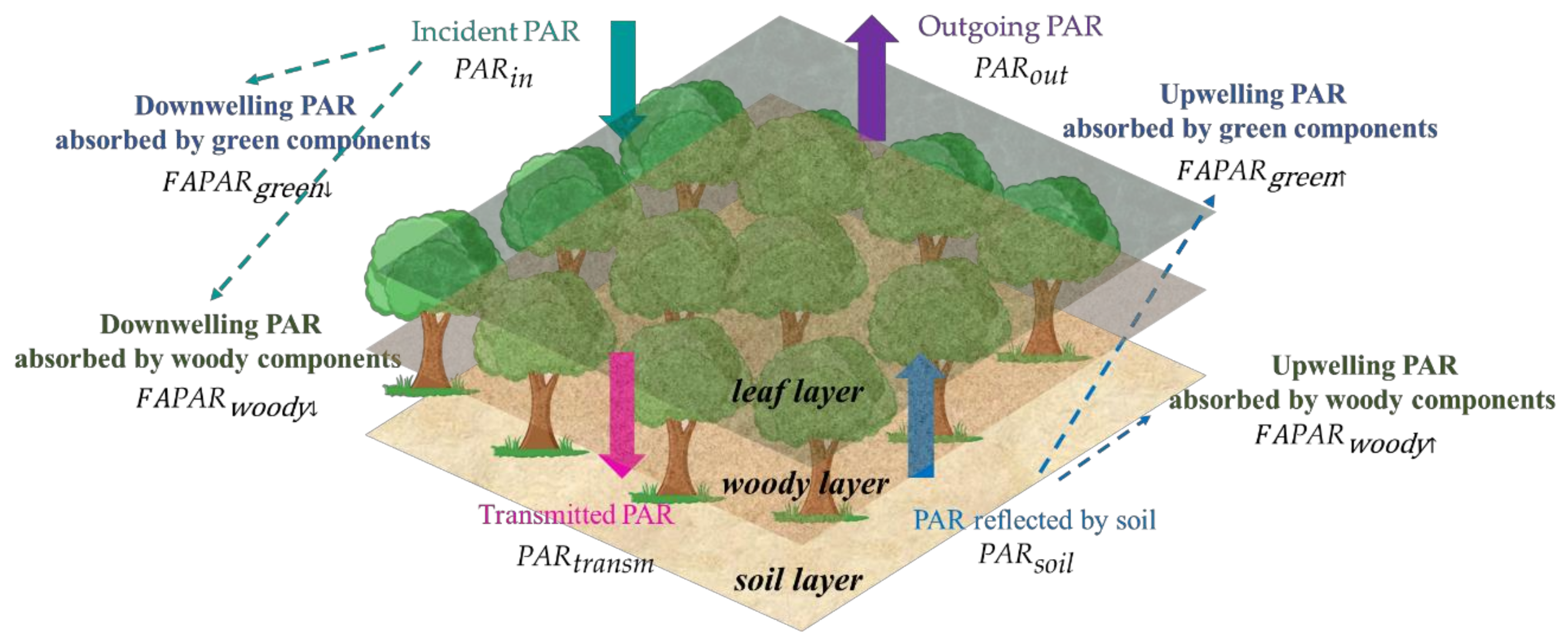
2.3.1. The Triple-Source Leaf–Wood–Soil Layer Model

A triple-source leaf–wood–soil layer model (TriLay) was developed to model the radiation transfer within the vegetation–soil system—this model is illustrated as Figure 3.
In this study, we used the layer approach to illustrate the distribution of leaves and soil in the whole canopy, which is consistent with the approach used in our previous study [15]. The layer approach assumes that the canopy consists only of green components and woody components and that all leaves are found above the canopy. The NSM model [15] was then used to simulate the canopy albedo.
The fraction of PAR absorbed by the canopy, F A P A R c a n o p y , can be separated into the fraction of PAR absorbed by the canopy for the downwelling radiation ( F A P A R c a n o p y ) and that for the upwelling radiation reflected from the soil background ( F A P A R c a n o p y ):
F A P A R c a n o p y = F A P A R c a n o p y + F A P A R c a n o p y
where F A P A R c a n o p y describes the fraction of downwelling radiation absorbed within the canopy assuming the soil background is dark, and F A P A R c a n o p y describes the fraction of upwelling radiation absorbed within the canopy due to the interaction between the ground (soil and understory) and the canopy. A point worth emphasizing is that, assuming a black soil background, the F A P A R c a n o p y is equal to the   F A P A R c a n o p y .
Therefore, F A P A R c a n o p y can be given by:
F A P A R c a n o p y = ( 1 τ P A I ) ( 1 A l b e d o p u r e F V C )
where τ P A I is the transmittance of the whole canopy, which contains green and woody parts, F V C is the fraction of vegetation cover, and A l b e d o p u r e is the visible (VIS) albedo for pure vegetation, which is represented by the VIS albedo for vegetation with a “saturated” LAI value (e.g., LAI ≥ 6) [14]. According to the statistical results by Liu et al. [15], A l b e d o p u r e was set to 0.025 (for white-sky conditions) and 0.020 (for black-sky conditions) for all woody vegetation types (including evergreen needleleaf forest, evergreen broadleaf forest, deciduous needleleaf forest, and deciduous broadleaf forest).
τ P A I can be calculated as the product of τ L A I and τ W A I , and the directional transmittance can be determined using the gap fraction model [16,53,54]:
τ P A I = τ L A I × τ W A I
τ L A I = e k 1 × G ( θ ) × C I × L A I / cos ( θ )
τ W A I = e k 2 × G ( θ ) × C I × W A I / cos ( θ )
where L A I and W A I are the leaf area index and woody area index, respectively, k 1 and k 2 are extinction coefficients for the green components and woody components, respectively, and θ is the solar zenith angle. k 1 can be determined using the leaf absorptance in the VIS band and was set to 0.88 based on simulations made using the PROSPECT-5 model and also the Leaf optical properties experiment 93 (LOPEX’93) and Leaf Optical Properties Database (an experiment conducted at the National Institute for Agricultural Research in Angers, France in June 2003) [55,56,57]. The woody components were assumed to be opaque with a constant extinction coefficient ( k 2 ) of 0.91 based on the simulated LESS data. G ( θ ) is the projection of the unit foliage area on the plane perpendicular to the solar incident direction, θ . For green leaves, G ( θ ) is normally given a value of 0.5 for canopies with a spherical leaf angle distribution. For woody components, we assuming the woody components have the same angular distribution as green leaves, which also assumed by Chen et al. [58], Kucharik et al. [59], and Sea et al. [60]. CI is the clumping index; we also assume the same CI values for both green leaves and woody components based on the findings of Chen et al. [61] and Zou et al. [62].
The gap fraction model is also used to calculate FVC for a fixed solar zenith angle of 0° and a fixed value of 1 for the leaf extinction coefficient:
F V C = 1 e G ( θ ) × L A I × C I
Similarly,   F A P A R c a n o p y can be calculated as follows:
F A P A R c a n o p y = ( 1 τ P A I ) ( 1 A l b e d o p u r e FVC )   τ P A I w s A l b e d o s o i l
where A l b e d o s o i l is the soil visible albedo, which can be generated by the NSM model proposed by Liu et al. [15]. τ P A I w s is the canopy transmittance under white-sky conditions, which can be calculated as the product of the white-sky transmittance of leaves ( τ L A I w s ) and the white-sky transmittance of woody components ( τ W A I w s ):
τ L A I w s = 2 × 0 π 2 ( e k 1 × G ( θ ) × L A I × C I / cos ( θ ) ) × sin ( θ ) × cos ( θ ) d θ
τ W A I w s = 2 × 0 π 2 ( e k 2 × G ( θ ) × W A I × C I / cos ( θ ) ) × sin ( θ ) × cos ( θ ) d θ
τ P A I w s = τ L A I w s × τ W A I w s

2.3.2. Determination of Woody Area Index

In general, it is expensive and time-consuming to make accurate estimates of the woody area index (WAI), and destructive sampling is often the only option available for the quantification of the WAI in tropical evergreen forests [63]. Therefore, for generating global F A P A R g r e e n datasets, the use of accurate estimates of WAI is unrealistic. Hence, in this study, we aimed to determine the global WAI using MCD15A2H LAI data and assumed that the WAI was constant within a given year.
First, we assumed that the woody-to-total area ratio is measured during the peak growth stage (July–August–September, JAS) when the LAI has its maximum value for the year. The woody-to- total area ratio was determined according to the forest types listed in the MODIS land cover product (MCD12Q1), including evergreen needleleaf forest (ENF), evergreen broadleaf forest (EBF), deciduous broadleaf forest (DBF), deciduous needleleaf forest (DNF) and mixed forest (MF). Therefore, WAI values for different forest vegetation types were calculated using a simple linear relationship between the plant area index (PAI) and the WAI:
W A I = P A I × r a t i o w o o d y = L A I m a x 1 r a t i o w o o d y × r a t i o w o o d y
where r a t i o w o o d y is the mean value of the woody-to-total area ratio for various forest types, as given in the literature [58,64,65]. L A I m a x is the maximum value of LAI within a given year; this was acquired from MCD15A2H LAI products.

2.3.3. Separating F A P A R g r e e n and F A P A R w o o d y from F A P A R c a n o p y

In a similar way to Equation (1), the fraction of PAR absorbed by the green and woody components can also be separated into the fraction of PAR absorbed by the canopy for the downwelling radiation and that for the upwelling radiation reflected from the soil background. Firstly F A P A R c a n o p y is split into F A P A R g r e e n and F A P A R w o o d y :
F A P A R c a n o p y = F A P A R g r e e n + F A P A R w o o d y
where F A P A R g r e e n and F A P A R w o o d y can be obtained as
F A P A R g r e e n = F A P A R c a n o p y × r a t i o g r e e n × w 1
F A P A R w o o d y = F A P A R c a n o p y × r a t i o w o o d y × w 2
where r a t i o g r e e n and r a t i o w o o d y are the ratio of leaf area index to plant area index and woody area index to plant area index, respectively. w 1 and w 2 are the weighting coefficients for the green (i.e., photosynthetic) and woody components in terms of the radiation transfer within the canopy. The terms involved in equations (10) and (11) can be given as:
  r a t i o g r e e n = L A I P A I
r a t i o w o o d y = W A I P A I
w 2 = w 1 × τ L A I
w 1 × r a t i o g r e e n + w 2 × r a t i o w o o d y = 1
F A P A R g r e e n and F A P A R w o o d y can then be obtained by solving equations (13)–(18):
F A P A R g r e e n = r a t i o g r e e n × F A P A R c a n o p y r a t i o g r e e n + τ L A I × r a t i o w o o d y
F A P A R w o o d y = r a t i o w o o d y × F A P A R c a n o p y × τ L A I r a t i o g r e e n + τ L A I × r a t i o w o o d y
Similarly, F A P A R g r e e n and F A P A R w o o d y can also be acquired:
F A P A R g r e e n = r a t i o g r e e n × F A P A R c a n o p y × τ W A I r a t i o w o o d y + τ W A I × r a t i o g r e e n
F A P A R w o o d y = r a t i o w o o d y × F A P A R c a n o p y r a t i o w o o d y + τ W A I × r a t i o g r e e n
Finally, F A P A R g r e e n and F A P A R w o o d y can be calculated as:
F A P A R g r e e n = F A P A R g r e e n + F A P A R g r e e n
F A P A R w o o d y = F A P A R w o o d y + F A P A R w o o d y

3. Results

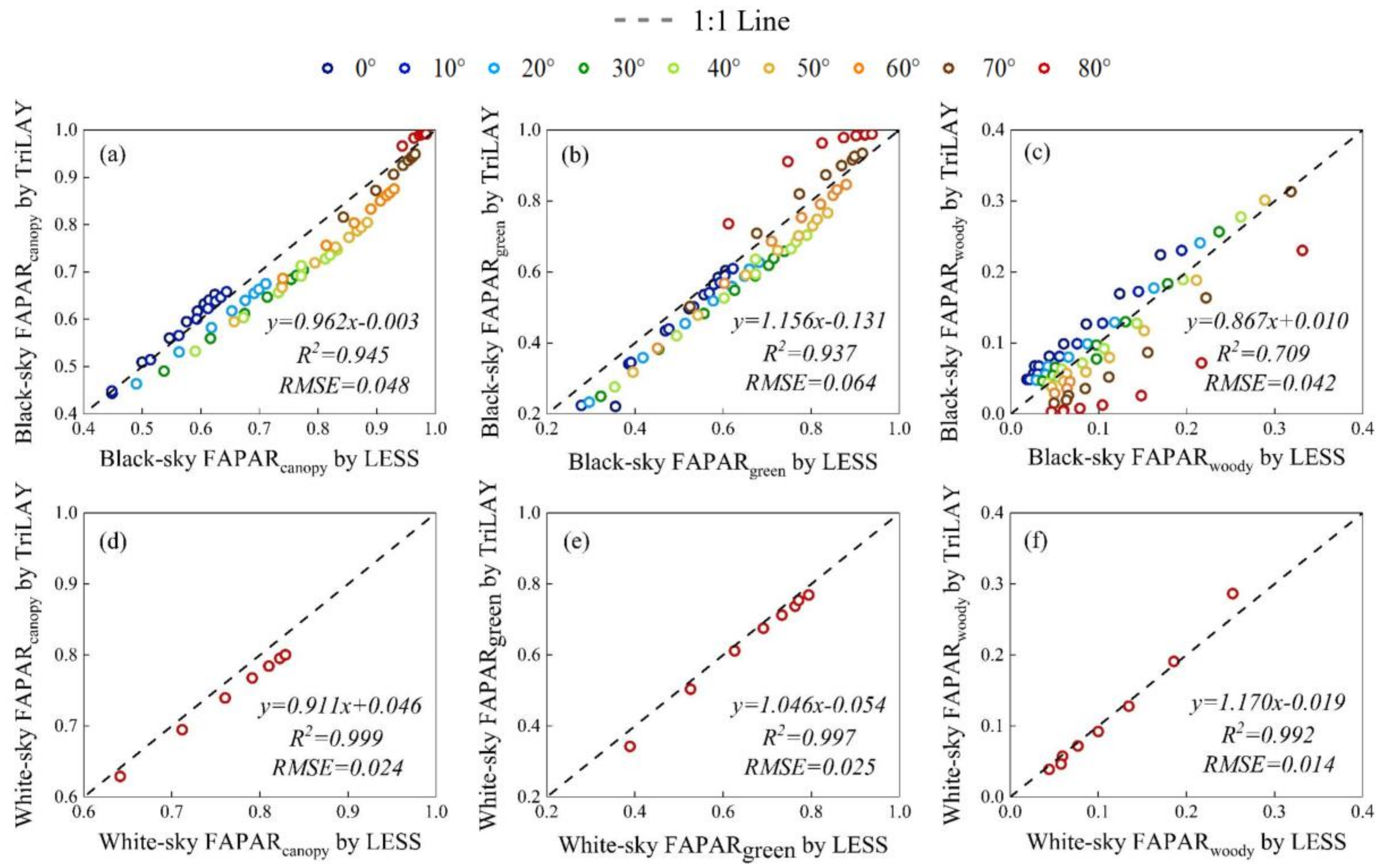
3.1. Validation of the TriLay Method using Simulations made by the LESS Model

It is too challenging to obtain in-situ measurements of F A P A R g r e e n for forests, and so the simulated dataset (Table 1) derived using the LESS model was used for the validation of the TriLay model. Seventy-two black-sky simulations of F A P A R c a n o p y , F A P A R g r e e n , and F A P A R w o o d y together with eight white-sky simulations were available for validation.
Figure 4 illustrates the validation results for F A P A R c a n o p y , F A P A R g r e e n , and F A P A R w o o d y . The estimated and simulated FAPAR values are distributed close to the 1:1 line. Also, it can be seen that the TriLay approach can produce accurate estimates of F A P A R c a n o p y , giving Root Mean Square Error (RMSEs) of 0.048 and 0.024 for black-sky and white-sky conditions, respectively, as against the LESS-simulated values. The corresponding R2 values are 0.945 and 0.999. For F A P A R g r e e n , the validation results give RMSEs of 0.064 and 0.025, respectively, for black-sky and white-sky FAPAR. Finally, it can be seen that F A P A R w o o d y can also be accurately estimated: the RMSE and R2 values are 0.042 and 0.709, respectively, for black-sky conditions, and 0.014 and 0.992 for white-sky conditions. These results show that the TriLay approach can be used to accurately estimate F A P A R c a n o p y , F A P A R g r e e n , and F A P A R w o o d y for forest land cover types.
Furthermore, as illustrated in Figure 4b, there is a slight underestimation for F A P A R g r e e n at smaller SZAs (0°–60°) and a slight overestimation for larger SZAs (70°–80°). From Figure 4c, it can be seen that F A P A R w o o d y is also slightly underestimated at smaller SZAs (0°–40°) and overestimated at larger angles (50°–80°).

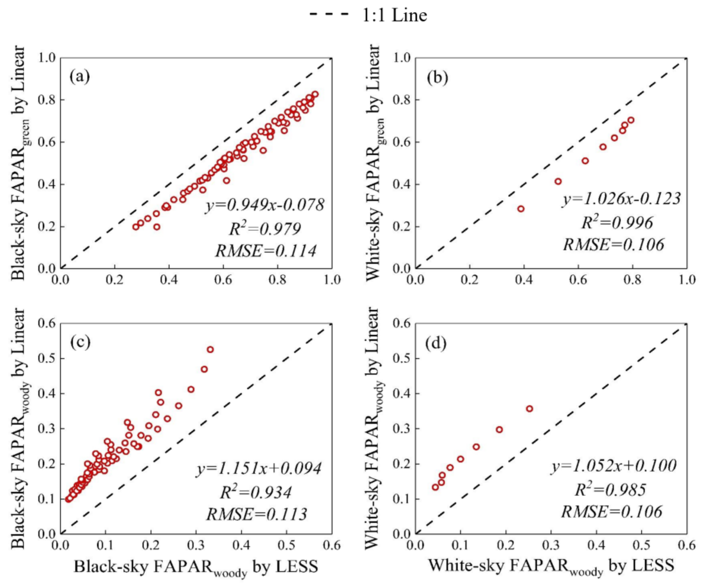
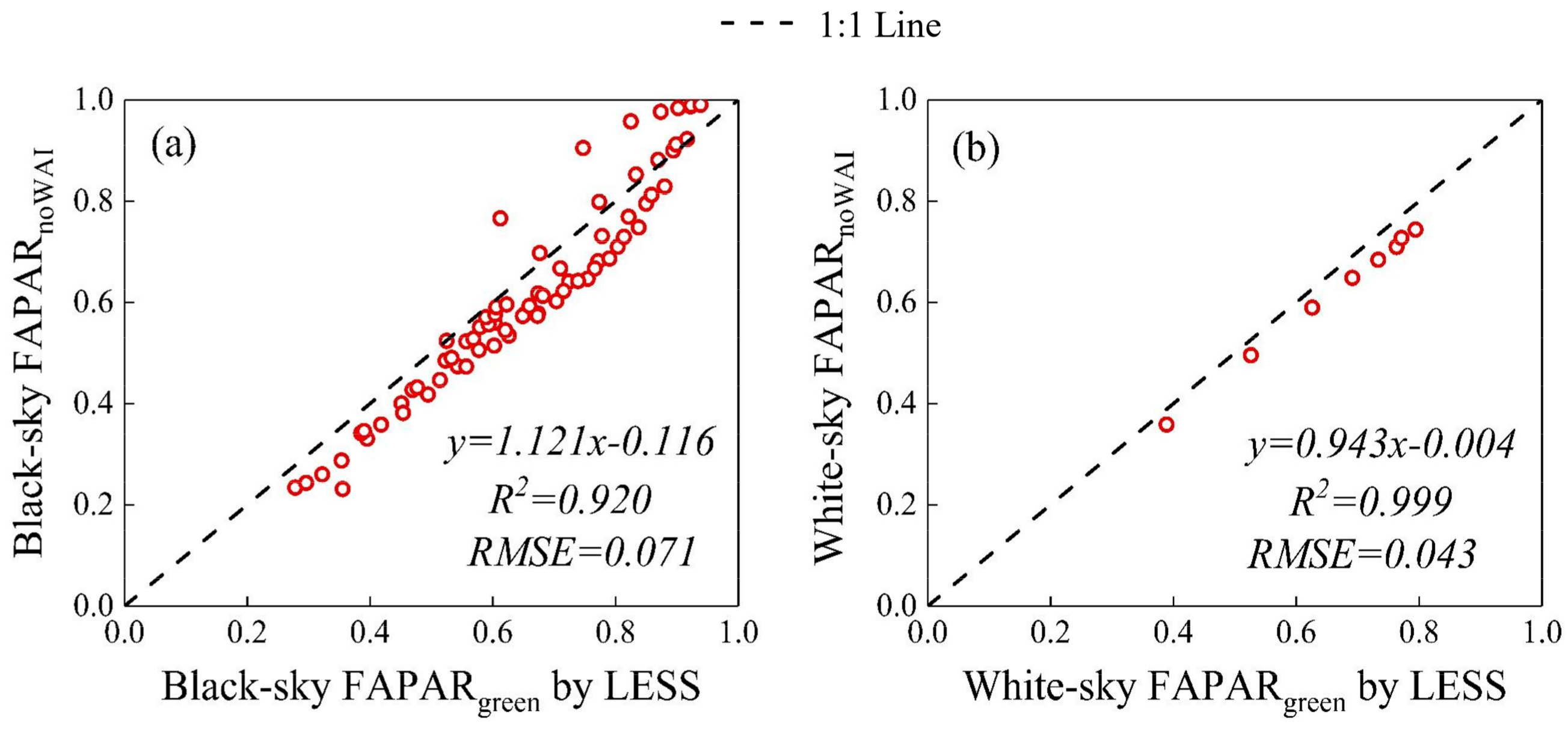
3.2. Comparison of Different Methods using the LESS Simulations

Hall et al. [38] estimated F A P A R g r e e n based on a simple linear relationship between F A P A R c a n o p y and F A P A R g r e e n . They used the ratio L A I g r e e n / L A I t o t a l to determine F A P A R g r e e n :
F A P A R g r e e n = F A P A R c a n o p y × L A I g r e e n t o t a l   L A I
where total LAI is the PAI mentioned above. In order to test the accuracy of the linear mixture method, we also validated the F A P A R g r e e n estimated by the linear mixture method [38] using LESS-simulated data.
Figure 5 shows the accuracy assessment results for the linear mixture method. The results show a noticeable underestimation for F A P A R g r e e n and a huge overestimation for F A P A R w o o d y . Although the FAPARs retrieved using the linear mixture method are highly correlated with the LESS simulation, with R2 values of 0.979, 0.996 for F A P A R g r e e n , and 0.934, 0.985 for F A P A R w o o d y under black-sky and white-sky conditions, the corresponding RMSE values are much higher than those found using our TriLay approach—0.114, 0.106 for F A P A R g r e e n as against 0.064, 0.025, and 0.113, 0.106 for F A P A R w o o d y as against 0.042, 0.014 under the black-sky and white-sky conditions, respectively.
The FAPAR values derived without considering the woody components ( F A P A R n o W A I ) were also validated using the LESS simulations; the results are shown in Figure 6. These results give an RMSE of 0.071 and R2 of 0.920 for the black-sky conditions and the corresponding values of 0.043 and 0.999 for the white-sky conditions. Although the R2 values are higher, the RMSEs are still greater than those found using the TriLay approach.
In order to further compare the performances of different methods, we also calculated the bias for F A P A R g r e e n , F A P A R w o o d y , and F A P A R n o W A I using the LESS-simulated FAPAR values. Table 2 summarizes the retrieval accuracy for these three methods. The results show that the TriLay method gave the best FAPAR retrieval results, having the smallest bias and RMSE values (RMSE = 0.064 and 0.025, and bias = −6.02%, −4.04% for F A P A R g r e e n under black-sky and white-sky conditions, respectively).

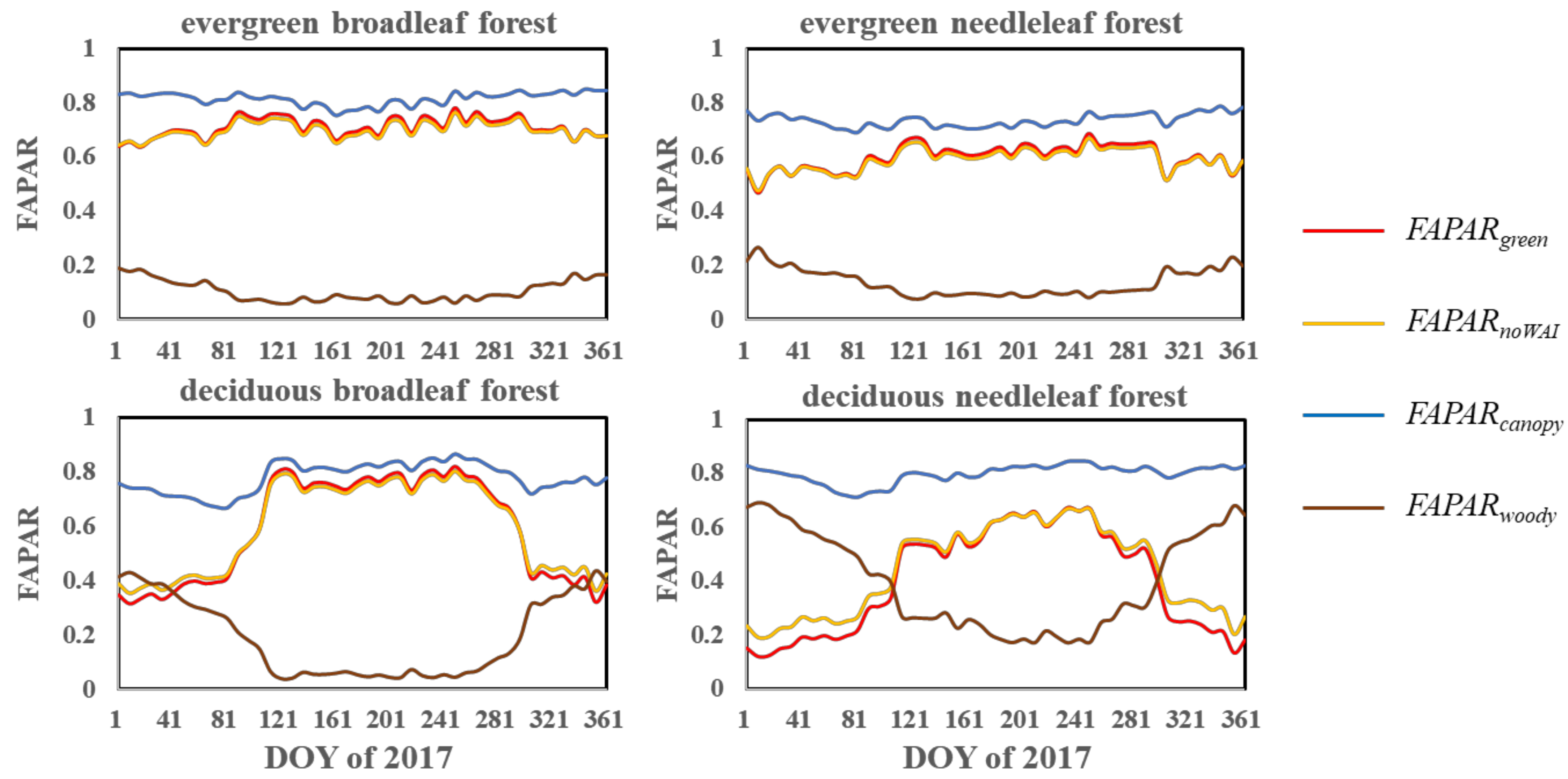
3.3. Temporal Variations in Different FAPAR Products

Using the TriLay approach, black-sky and white-sky products, including F A P A R g r e e n , F A P A R w o o d y , and F A P A R c a n o p y , and also FAPAR without woody components ( F A P A R n o W A I ), were generated for tile h10v05 in 2017. The black-sky FAPAR products were determined according to the SZA values at 10:30 am local time (the overpass time of the Terra satellite).
To investigate the seasonal variations in F A P A R g r e e n and the other FAPAR products, only the mean black-sky FAPAR values were calculated for the different forest vegetation types, as shown in Figure 7. The proportion of black-sky F A P A R g r e e n in F A P A R c a n o p y and F A P A R n o W A I , and also the bias between the black-sky F A P A R g r e e n , F A P A R c a n o p y , and F A P A R n o W A I were calculated for different periods during 2017 in order to analyze the differences between different black-sky FAPAR products, as well as to quantify the contribution of the woody components for several forest vegetation types (deciduous broadleaf forest, deciduous needleleaf forest, evergreen broadleaf forest, and evergreen needleleaf forest, referred to as DBF, DNF, EBF, and ENF, respectively). The results are illustrated in Figure 8 and Table 3.
In general, the black-sky F A P A R g r e e n and F A P A R n o W A I exhibit typical seasonal variations for the selected forest types, with low values during the early and late period (January–February–March (JFM) and October–November–December (OND)) and high values during the peak growth stage (July–August–September (JAS)). The black-sky F A P A R c a n o p y is obviously higher than the black-sky F A P A R g r e e n during the whole year and has a much smaller seasonal variation. The black-sky F A P A R w o o d y behaves in the opposite way; for deciduous seasons (JFM and OND), F A P A R w o o d y is close to or higher than its value during the peak growth stage (JAS) because the black-sky FAPAR increases with increasing SZA value. (The mean SZA at 10:30 am varies from 22.98° (22 December) to 62.25° (22 June) within tile h10v05.)
The black-sky F A P A R g r e e n is about 52.59% and 60.60% of the black-sky F A P A R c a n o p y for deciduous broadleaf forest during JFM and OND, respectively; the corresponding figures for deciduous needleleaf forest are only about 23.86% and 35.75%. During the peak growth stage (JAS), the black-sky F A P A R g r e e n is about 93.36%, 75.02%, 90.93% and 87.14% of F A P A R c a n o p y for DBF, DNF, EBF, and ENF, respectively.
There are also small discrepancies between F A P A R n o W A I and F A P A R g r e e n (Figure 8). In particular, for deciduous needleleaf forests, the black-sky F A P A R n o W A I is overestimated by 38.30% and 28.46% during the early and late stages of the year (JFM and OND). For evergreen forests, the difference can be neglected as there is only a very slight underestimation of 0.68% to 2.39% during the whole year.

4. Discussion

4.1. Uncertainty in Determining WAI

Currently, methods for measuring the woody area index (WAI) and woody-to-total area ratio can be classified into direct methods (e.g., destructive sampling) and indirect methods [66]. However, both the direct and indirect methods can only be applied at small scales and to a limited range of vegetation types. In this study, we used a constant value of the woody-to-total area ratio for each forest type and derived the WAI from the PAI value for the peak growth stage. We obtained woody-to-total area ratios for different forest types (ENF, EBF, DBF, and DNF) from an extensive literature review [58,64,65,66,67]—the statistical metrics, including the mean, standard deviation, and coefficient of variation, are shown in Table 4. These results show that the woody-to-total area ratios for different forest types vary from 0.158 to 0.3. The variation in this ratio within each of the forest types is also large—10.00% to 82.22%. Therefore, the woody-to-total area ratio not only varies with the forest type but also changes a lot for each individual forest type. This means that there is definitely some uncertainty due to these factors. Even so, Zou et al. [66] showed that the woody-to-total area ratio is relatively stable for the same forest stand and thus the assumption of a fixed woody-to-total area ratio for each forest type is reasonable. Differences in in situ measurement methods can also contribute to the variation in the ratio for a given forest type. The retrieval of F A P A R g r e e n can thus be improved if an accurate woody-to-total area ratio dataset is available.

4.2. Uncertainty Caused by the Use of Fixed Values of the Extinction Coefficients and A l b e d o p u r e

The canopy directional transmittance can be determined using the gap fraction model [16,53,54]. Splitting the canopy into green components and woody components requires that the transmittances are also calculated separately. For the green components, the leaf absorptance at the VIS band varies from 0.79 to 0.94 as the chlorophyll content varies (from 20 to 100 μg/cm2 under natural conditions), according to figures obtained using the PROSPECT-5 model [56,57]. Also, because no remote sensing leaf chlorophyll content product is available, the extinction coefficient for leaves ( k 1 ) was assumed to have a fixed value of 0.88 (corresponding to a chlorophyll content of 35 μg/cm2 [15]). For the extinction coefficient of woody components ( k 2 ), we also used a fixed value of 0.91, based on the data simulated by LESS (a needleleaf forest scene). However, Suwa et al. [68] reported a smaller extinction coefficient of 0.77 for brighter woody stems. Therefore, the extinction coefficient of woody components may vary with forest type, and thus the use of a fixed value for k 2 is also a source of error. At present, it is still very challenging to determine extinction coefficients for different forest canopy types.
In addition, a fixed value of A l b e d o p u r e was used in the TriLay model for woody vegetation types (i.e., ENF, EBF, DBF, and DNF), and was approximated based on the dense vegetation [15]. According to the statistical results obtained from the MCD43A3 albedo product by Liu et al. [15], the visible albedo of dense vegetation with a “saturated” LAI value (e.g., LAI = 6) is very low and stable, with a mean value of 0.025 and a variance of 0.007 for white-sky condition, and a mean value of 0.020 and a variance of 0.006 for black-sky conditions. Therefore, the use of the prior VIS albedo values for “pure” vegetation may introduce a very small error, but it should be negligible [14].

4.3. Setting the Clumping Index for Photosynthetic and Woody Components

The clumping index characterizes the grouping of foliage within distinct canopy structures (such as tree crowns, shrubs, and row crops) relative to a random spatial distribution of leaves and is an important structural parameter for plant canopies that can influence canopy radiation regimes [49]. In our TriLay approach, the clumping index for woody components was assumed to be the same as for green leaves, and so is another definite source of error [69]. However, it is currently challenging to obtain the clumping effects of woody components within forest canopies [62]. Furthermore, Chen et al. [61] indicated that the clumping of shoots in branches has a similar effect to the clumping of leaves within shoots. What’s more, Zou et al. [62] found that the differences between the estimated CI for canopy and woody components was below 6% at the zenithal ranges of 0 ° –75 ° , and the difference was only 2% in the range of 30 ° –60 ° , which is quite small at most medium zenithal ranges thus can represent most actual conditions. Based on these results and the unavailability of CI datasets for forest canopies at large scales, we directly used the value of CI from Jiao et al. [49] to describe the clumping effect for both leaves and woody components. Therefore, the use of the same clumping index for both leaves and woody components is reasonable and credibe enough.

5. Conclusions

In this paper, a triple-source leaf–wood–soil layer (TriLay) method for separating F A P A R g r e e n and F A P A R w o o d y from F A P A R c a n o p y using the MODIS LAI, land cover, and non-linear spectral mixture model (NSM)-retrieved soil albedo [15] together with global CI products [49] was proposed.
According to the validation carried out using LESS-simulated FAPAR values, the TriLay F A P A R g r e e n was more accurate (R2 = 0.937, RMSE = 0.064 and bias = −6.02% for black-sky conditions; R2 = 0.997, RMSE = 0.025 and bias = −4.04% for white-sky conditions) than the traditional linear method (R2 = 0.979, RMSE = 0.114 and bias = −18.04% for black-sky conditions; R2 = 0.996, RMSE = 0.106 and bias = −16.93% for white-sky conditions), and also more accurate than FAPAR obtained without the consideration of woody components ( F A P A R n o W A I ) (R2 = 0.920, RMSE = 0.071 and bias = −7.14% for black-sky conditions; R2 = 0.999, RMSE = 0.043 and bias = −6.41% for white-sky conditions). A comparison of the results for black-sky F A P A R g r e e n against F A P A R n o W A I and F A P A R c a n o p y showed that the discrepancies between the black-sky F A P A R g r e e n and other FAPAR products could not be ignored for forest types. In particular, for deciduous needleleaf forest, the black-sky F A P A R g r e e n contributed only about 23.86% and 35.75% of F A P A R c a n o p y during the early and late stages (JFM and OND) of the year, respectively, and 75.02% during the peak growth stage (JAS). There were also smaller discrepancies between the black-sky F A P A R n o W A I and F A P A R g r e e n . For deciduous needleleaf forests, in particular, the black-sky F A P A R n o W A I was overestimated by 38.30% and 28.46%, respectively, during the early and late stages of the year (JFM and OND).
Overall, this study provides a new method for partitioning F A P A R c a n o p y into F A P A R g r e e n and F A P A R w o o d y for forest types and will improve the understanding of energy exchange within the canopy. In addition, the exclusion of the contribution of woody components may certainly improve the accuracy of the F A P A R g r e e n estimates for forest types, which is significant in terms of the better modeling of vegetation photosynthesis.

Author Contributions

Conceptualization—S.C. and L.L.; methodology—S.C. and L.L.; software—S.C., X.Z. and X.C.; validation—S.C., Y.X. and D.X.; formal analysis—S.C. and X.Q.; investigation—S.C. and L.L.; resources—S.C.; writing—original draft preparation—S.C.; writing—review and editing—L.L. and X.L.

Funding

This research was funded by the National Key Research and Development Program of China, grant number 2017YFA0603001, the Key Research Program of the Chinese Academy of Sciences (ZDRW-ZS-2019-1), the National Natural Science Foundation of China (41825002).

Acknowledgments

The authors gratefully acknowledge the CI products provided by Ziti Jiao at Beijing Normal University, and the MODIS products obtained from the Land Products Land Processes Distributed Active Archive Center (LP DAAC).

Conflicts of Interest

The authors declare no conflict of interest.

References

  1. Monteith, J.L. Vegetation and the atmosphere. Volume 1. Principles. J. Appl. Ecol. 1977, 14, 655. [Google Scholar]
  2. Sellers, P.; Dickinson, R.; Randall, D.; Betts, A.; Hall, F.; Berry, J.; Collatz, G.; Denning, A.; Mooney, H.; Nobre, C. Modeling the exchanges of energy, water, and carbon between continents and the atmosphere. Science 1997, 275, 502–509. [Google Scholar] [CrossRef] [PubMed]
  3. Prince, S.D.; Goward, S.N. Global primary production: A remote sensing approach. J. Biogeogr. 1995, 22, 815–835. [Google Scholar] [CrossRef]
  4. Ruimy, A.; Dedieu, G.; Saugier, B. Turc: A diagnostic model of continental gross primary productivity and net primary productivity. Glob. Biogeochem. Cycles 1996, 10, 269–285. [Google Scholar] [CrossRef]
  5. Running, S.W.; Nemani, R.R.; Heinsch FAZhao, M.S.; Reeves, M.; Hashimoto, H. A continuous satellite-derived measure of global terrestrial primary production. Bioscience 2004, 54, 547–560. [Google Scholar] [CrossRef]
  6. Potter, C.S.; Randerson, J.T.; Field, C.B.; Matson, P.A.; Vitousek, P.M.; Mooney, H.A.; Klooster, S.A. Terrestrial ecosystem production: A process model based on global satellite and surface data. Glob. Biogeochem. Cycles 1993, 7, 811–841. [Google Scholar] [CrossRef]
  7. Verhoef, W.; Bach, H. Coupled soil-leaf-canopy and atmosphere radiative transfer modeling to simulate hyperspectral multi-angular surface reflectance and toa radiance data. Remote Sens. Environ. 2007, 109, 166–182. [Google Scholar] [CrossRef]
  8. Liu, R.; Huang, W.; Ren, H.; Yang, G.; Xie, D.; Wang, J. Photosynthetically active radiation vertical distribution model in maize canopy. Trans. Chin. Soc. Agric. Eng. 2011, 27, 115–121. [Google Scholar]
  9. Li, W.; Fang, H. Estimation of direct, diffuse, and total fpars from landsat surface reflectance data and ground-based estimates over six fluxnet sites. J. Geophys. Res. Biogeosci. 2015, 120, 96–112. [Google Scholar] [CrossRef]
  10. Myneni, R.B.; Ramakrishna, R.; Nemani, R.; Running, S.W. Estimation of global leaf area index and absorbed par using radiative transfer models. IEEE Trans. Geosci. Remote Sens. 2002, 35, 1380–1393. [Google Scholar] [CrossRef]
  11. Knyazikhin, Y.; Martonchik, J.V.; Diner, D.J.; Myneni, R.B.; Verstraete, M.; Pinty, B.; Gobron, N. Estimation of vegetation canopy leaf area index and fraction of absorbed photosynthetically active radiation from atmosphere-corrected misr data. J. Geophys. Res. Space Phys. 1998, 103, 32257–32275. [Google Scholar] [CrossRef]
  12. Tian, Y.; Zhang, Y.; Knyazikhin, Y.; Myneni, R.B.; Glassy, J.M.; Dedieu, G.; Running, S.W. Prototyping of modis lai and fpar algorithm with lasur and landsat data. IEEE Trans. Geosci. Remote Sens. 2000, 38, 2387–2401. [Google Scholar] [CrossRef]
  13. Gobron, N.; Pinty, B.; Verstraete, M.M.; Govaerts, Y. A semidiscrete model for the scattering of light by vegetation. J. Geophys. Res. Space Phys. 1997, 102, 9431–9446. [Google Scholar] [CrossRef]
  14. Xiao, Z.; Liang, S.; Rui, S.; Wang, J.; Bo, J. Estimating the fraction of absorbed photosynthetically active radiation from the modis data based glass leaf area index product. Remote Sens. Environ. 2015, 171, 105–117. [Google Scholar] [CrossRef]
  15. Liu, L.; Zhang, X.; Xie, S.; Liu, X.; Song, B.; Chen, S.; Peng, D. Global white-sky and black-sky fapar retrieval using the energy balance residual method: Algorithm and validation. Remote Sens. 2019, 11, 1004. [Google Scholar] [CrossRef]
  16. Chen, J.M. Canopy architecture and remote sensing of the fraction of photosynthetically active radiation absorbed by boreal conifer forests. IEEE IEEE Trans. Geosci. Remote Sens. 1996, 34, 1353–1368. [Google Scholar] [CrossRef]
  17. Chen, L.; Liu, Q.; Fan, W.; Li, X.; Xiao, Q.; Yan, G.; Tian, G. A bi-directional gap model for simulating the directional thermal radiance of row crops. Sci. China 2002, 45, 1087–1098. [Google Scholar] [CrossRef]
  18. Fan, W.; Yuan, L.; Xu, X.; Chen, G.; Zhang, B. A new fapar analytical model based on the law of energy conservation: A case study in china. IEEE J. Sel. Top. Appl. Earth Obs. Remote Sens. 2014, 7, 3945–3955. [Google Scholar] [CrossRef]
  19. Fang, H.; Liang, S.; Mcclaran, M.P.; Leeuwen, W.J.D.V.; Drake, S.; Marsh, S.E.; Thomson, A.M.; Izaurralde, R.C.; Rosenberg, N.J. Biophysical characterization and management effects on semiarid rangeland observed from landsat etm+ data. IEEE Trans. Geosci. Remote Sens. 2005, 43, 125–134. [Google Scholar] [CrossRef]
  20. Myneni, R.B.; Hoffman, S.; Knyazikhin, Y.; Privette, J.L.; Glassy, J.; Tian, Y.; Wang, Y.; Song, X.; Zhang, Y.; Smith, G.R.; et al. Global products of vegetation leaf area and fraction absorbed par from year one of modis data. Remote Sens. Environ. 2002, 83, 214–231. [Google Scholar] [CrossRef]
  21. Knyazikhin, Y.; Martonchik, J.; Myneni, R.B.; Diner, D.; Running, S.W. Synergistic algorithm for estimating vegetation canopy leaf area index and fraction of absorbed photosynthetically active radiation from modis and misr data. J. Geophys. Res. Space Phys. 1998, 103, 32257–32275. [Google Scholar] [CrossRef]
  22. Baret, F.; Hagolle, O.; Geiger, B.; Bicheron, P.; Miras, B.; Huc, M.; Berthelot, B.; Niño, F.; Weiss, M.; Samain, O. Lai, fapar and fcover cyclopes global products derived from vegetation: Part 1: Principles of the algorithm. Remote Sens. Environ. 2009, 110, 275–286. [Google Scholar] [CrossRef]
  23. Plummer, S.; Arino, O.; Simon, M.; Steffen, W. Establishing a earth observation product service for the terrestrial carbon community: The globcarbon initiative. Mitig. Adapt. Strat. Glob. Chang. 2006, 11, 97–111. [Google Scholar] [CrossRef]
  24. Gobron, N.; Pinty, B.; Verstraete, M.; Govaerts, Y. The MERIS Global Vegetation Index (MGVI): Description and preliminary application. Int. J. Remote Sens. 1999, 20, 1917–1927. [Google Scholar] [CrossRef]
  25. Pinty, B.; Clerici, M.; Andredakis, I.; Kaminski, T.; Taberner, M.; Verstraete, M.M.; Gobron, N.; Plummer, S.; Widlowski, J.-L. Exploiting the MODIS albedos with the Two-stream Inversion Package (JRC-TIP): 2. Fractions of transmitted and absorbed fluxes in the vegetation and soil layers. J. Geophys. Res. Space Phys. 2011, 116. [Google Scholar] [CrossRef] [Green Version]
  26. Disney, M.; Muller, J.-P.; Kharbouche, S.; Kaminski, T.; Voßbeck, M.; Lewis, P.; Pinty, B. A New Global fAPAR and LAI Dataset Derived from Optimal Albedo Estimates: Comparison with MODIS Products. Remote Sens. 2016, 8, 275. [Google Scholar] [CrossRef]
  27. Wang, Y.; Tian, Y.; Zhang, Y.; Elsaleous, N.; Knyazikhin, Y.; Vermote, E.; Myneni, R.B. Investigation of product accuracy as a function of input and model uncertainties—Case study with seawifs and modis lai/fpar algorithm. Remote Sens. Environ. 2000, 78, 299–313. [Google Scholar] [CrossRef]
  28. Camacho, F.; Cernicharo, J.; Lacaze, R.; Baret, F.; Weiss, M. GEOV1: LAI, FAPAR essential climate variables and FCOVER global time series capitalizing over existing products. Part 2: Validation and intercomparison with reference products. Remote Sens. Environ. 2013, 137, 310–329. [Google Scholar] [CrossRef]
  29. Gobron, N.; Pinty, B.; Aussedat, O.; Taberner, M.; Faber, O.; Melin, F.; Lavergne, T.; Robustelli, M.; Snoeij, P. Uncertainty estimates for the FAPAR operational products derived from MERIS—Impact of top-of-atmosphere radiance uncertainties and validation with field data. Remote Sens. Environ. 2008, 112, 1871–1883. [Google Scholar] [CrossRef]
  30. Fritsch, S.; Machwitz, M.; Ehammer, A.; Conrad, C.; Dech, S. Validation of the collection 5 MODIS FPAR product in a heterogeneous agricultural landscape in arid Uzbekistan using multitemporal RapidEye imagery. Int. J. Remote Sens. 2012, 33, 6818–6837. [Google Scholar] [CrossRef]
  31. Pickett-Heaps, C.A.; Canadell, J.; Briggs, P.R.; Gobron, N.; Haverd, V.; Paget, M.J.; Pinty, B.; Raupach, M.R. Evaluation of six satellite-derived Fraction of Absorbed Photosynthetic Active Radiation (FAPAR) products across the Australian continent. Remote Sens. Environ. 2014, 140, 241–256. [Google Scholar] [CrossRef]
  32. Tao, X.; Liang, S.; Wang, D. Assessment of five global satellite products of fraction of absorbed photosynthetically active radiation: Intercomparison and direct validation against ground-based data. Remote Sens. Environ. 2015, 163, 270–285. [Google Scholar] [CrossRef]
  33. Gitelson, A.A.; Peng, Y.; Arkebauer, T.J.; Suyker, A.E. Productivity, absorbed photosynthetically active radiation, and light use efficiency in crops: Implications for remote sensing of crop primary production. J. Plant Physiol. 2015, 177, 100–109. [Google Scholar] [CrossRef] [PubMed] [Green Version]
  34. Tewes, A.; Schellberg, J. Towards remote estimation of radiation use efficiency in maize using uav-based low-cost camera imagery. Agronomy 2018, 8, 16. [Google Scholar] [CrossRef]
  35. Miao, G.; Guan, K.; Xi, Y.; Bernacchi, C.J.; Masters, M.D. Sun-induced chlorophyll fluorescence, photosynthesis, and light use efficiency of a soybean field. J. Geophys. Res. Biogeosci. 2018, 123, 610–623. [Google Scholar] [CrossRef]
  36. Gitelson, A.A.; Arkebauer, T.J.; Suyker, A.E. Convergence of daily light use efficiency in irrigated and rainfed C3 and C4 crops. Remote Sens. Environ. 2018, 217, 30–37. [Google Scholar] [CrossRef]
  37. Asner, G.P.; Wessman, C.A.; Archer, S. Scale dependence of absorption of photosynthetically active radiation in terrestrial ecosystems. Ecol. Appl. 1998, 8, 1003–1021. [Google Scholar] [CrossRef]
  38. Hall, F.G.; Huemmrich, K.F.; Goetz, S.J.; Sellers, P.J.; Nickeson, J.E. Satellite remote sensing of surface energy balance: Success, failures, and unresolved issues in FIFE. J. Geophys. Res. Space Phys. 1992, 97, 19061–19089. [Google Scholar] [CrossRef]
  39. Zhang, Q.; Xiao, X.; Braswell, B.; Linder, E.; Baret, F.; Moore, B. Estimating light absorption by chlorophyll, leaf and canopy in a deciduous broadleaf forest using MODIS data and a radiative transfer model. Remote Sens. Environ. 2005, 99, 357–371. [Google Scholar] [CrossRef]
  40. Gitelson, A.A. Remote estimation of fraction of radiation absorbed by photosynthetically active vegetation: Generic algorithm for maize and soybean. Remote Sens. Lett. 2019, 10, 283–291. [Google Scholar] [CrossRef]
  41. Gitelson, A.A.; Peng, Y.; Arkebauer, T.J.; Schepers, J. Relationships between gross primary production, green LAI, and canopy chlorophyll content in maize: Implications for remote sensing of primary production. Remote Sens. Environ. 2014, 144, 65–72. [Google Scholar] [CrossRef]
  42. Gitelson, A.A.; Peng, Y.; Huemmrich, K.F. Relationship between fraction of radiation absorbed by photosynthesizing maize and soybean canopies and NDVI from remotely sensed data taken at close range and from MODIS 250m resolution data. Remote Sens. Environ. 2014, 147, 108–120. [Google Scholar] [CrossRef] [Green Version]
  43. Qi, J.; Xie, D.; Guo, D.; Yan, G. A large-scale emulation system for realistic three-dimensional (3-d) forest simulation. IEEE J. Sel. Top. Appl. Earth Obs. Remote Sens. 2017, 10, 4834–4843. [Google Scholar] [CrossRef]
  44. Myneni, R.; Knyazikhin, Y.; Park, T. MCD15A2H MODIS/Terra + Aqua leaf area index/FPAR 8-day L4 Global 500 m SIN Grid V006, NASA EOSDIS Land Processes DAAC. 2015. Available online: http://0-doi-org.brum.beds.ac.uk/10.5067/MODIS/MCD15A2H.006 (accessed on 12 September 2019).
  45. Vermote, E.; Vermeulen, A. Atmospheric correction algorithm: Spectral reflectances (mod09). ATBD Version 1999, 4, 1–107. [Google Scholar]
  46. Friedl, M.; McIver, D.; Hodges, J.; Zhang, X.; Muchoney, D.; Strahler, A.; Woodcock, C.; Gopal, S.; Schneider, A.; Cooper, A.; et al. Global land cover mapping from MODIS: Algorithms and early results. Remote Sens. Environ. 2002, 83, 287–302. [Google Scholar] [CrossRef]
  47. Friedl, M.A.; Sulla-Menashe, D.; Tan, B.; Schneider, A.; Ramankutty, N.; Sibley, A.; Huang, X. MODIS Collection 5 global land cover: Algorithm refinements and characterization of new datasets. Remote Sens. Environ. 2010, 114, 168–182. [Google Scholar] [CrossRef]
  48. Chen, J.; Menges, C.; Leblanc, S. Global mapping of foliage clumping index using multi-angular satellite data. Remote Sens. Environ. 2005, 97, 447–457. [Google Scholar] [CrossRef]
  49. Jiao, Z.; Dong, Y.; Schaaf, C.B.; Chen, J.M.; Roman, M.; Wang, Z.; Zhang, H.; Ding, A.; Erb, A.; Hill, M.J.; et al. An algorithm for the retrieval of the clumping index (CI) from the MODIS BRDF product using an adjusted version of the kernel-driven BRDF model. Remote Sens. Environ. 2018, 209, 594–611. [Google Scholar] [CrossRef]
  50. Liu, L.; Zhang, X. Dynamic Mapping of Broadband Visible Albedo of Soil Background at Global 500-m Scale from MODIS Satellite Products. In Land Surface and Cryosphere Remote Sensing IV; International Society for Optics and Photonics: Washington, DC, USA, 2018; p. 107770L. [Google Scholar]
  51. Irons, J.R.; Ranson, K.J.; Daughtry, C.S.T. Estimating big bluestem albedo from directional reflectance measurements. Remote Sens. Environ. 1988, 25, 185–199. [Google Scholar] [CrossRef]
  52. Carrer, D.; Meurey, C.; Ceamanos, X.; Roujean, J.L.; Calvet, J.C. Dynamic mapping of snow-free vegetation and bare soil albedos at global 1 km scale from 10-year analysis of modis satellite products. Remote Sens. Environ. 2014, 140, 420–432. [Google Scholar] [CrossRef]
  53. Widlowski, J.-L. On the bias of instantaneous FAPAR estimates in open-canopy forests. Agric. For. Meteorol. 2010, 150, 1501–1522. [Google Scholar] [CrossRef]
  54. Lhomme, J.-P.; Chehbouni, A. Comments on dual-source vegetation—Atmosphere transfer models. Agric. For. Meteorol. 1999, 94, 269–273. [Google Scholar] [CrossRef]
  55. Hosgood, B.; Jacquemoud, S.; Andreoli, G.; Verdebout, J.; Pedrini, G.; Schmuck, G. Leaf Optical Properties Experiment 93 (LOPEX93); Report EUR—16095-EN; Joint Research Centre, Institute for Remote Sensing Applications: Ispra, Italy; European Commission: Luxembourg, 1995. [Google Scholar]
  56. Jacquemoud, S.; Baret, F. PROSPECT: A model of leaf optical properties spectra. Remote Sens. Environ. 1990, 34, 75–91. [Google Scholar] [CrossRef]
  57. Féret, J.-B.; François, C.; Asner, G.P.; Gitelson, A.A.; Martin, R.E.; Bidel, L.P.; Ustin, S.L.; Le Maire, G.; Jacquemoud, S. PROSPECT-4 and 5: Advances in the leaf optical properties model separating photosynthetic pigments. Remote Sens. Environ. 2008, 112, 3030–3043. [Google Scholar] [CrossRef]
  58. Chen, J.M. Optically-based methods for measuring seasonal variation of leaf area index in boreal conifer stands. Agric. For. Meteorol. 1996, 80, 135–163. [Google Scholar] [CrossRef]
  59. Kucharik, C.J.; Norman, J.M.; Gower, S.T. Measurements of branch area and adjusting leaf area index indirect measurements. Agric. For. Meteorol. 1998, 91, 69–88. [Google Scholar] [CrossRef]
  60. Sea, W.B.; Choler, P.; Beringer, J.; Weinmann, R.A.; Hutley, L.B.; Leuning, R. Documenting improvement in leaf area index estimates from MODIS using hemispherical photos for Australian savannas. Agric. For. Meteorol. 2011, 151, 1453–1461. [Google Scholar] [CrossRef]
  61. Chen, J.M.; Leblanc, S.G. A four-scale bidirectional reflectance model based on canopy architecture. IEEE Trans. Geosci. Remote Sens. 1997, 35, 1316–1337. [Google Scholar] [CrossRef]
  62. Jie, Z.; Yan, G.; Ling, C. Estimation of canopy and woody components clumping indices at three mature. IEEE J. Sel. Top. Appl. Earth Obs. Remote Sens. 2015, 8, 1–10. [Google Scholar]
  63. Clark, D.B.; Olivas, P.C.; Oberbauer, S.F.; Clark, D.A.; Ryan, M.G. First direct landscape-scale measurement of tropical rain forest leaf area index, a key driver of global primary productivity. Ecol. Lett. 2008, 11, 163–172. [Google Scholar] [CrossRef]
  64. Zheng, G.; Ma, L.; Wei, H.; Eitel, J.U.H.; Moskal, L.M.; Zhang, Z. Assessing the contribution of woody materials to forest angular gap fraction and effective leaf area index using terrestrial laser scanning data. IEEE Trans. Geosci. Remote Sens. 2016, 54, 1475–1487. [Google Scholar] [CrossRef]
  65. Zou, J.; Zhuang, Y.; Chianucci, F.; Mai, C.; Lin, W.; Leng, P.; Luo, S.; Yan, B. Comparison of Seven Inversion Models for Estimating Plant and Woody Area Indices of Leaf-on and Leaf-off Forest Canopy Using Explicit 3D Forest Scenes. Remote Sens. 2018, 10, 1297. [Google Scholar] [CrossRef]
  66. Zou, J.; Yan, G.; Zhu, L.; Zhang, W. Woody-to-total area ratio determination with a multispectral canopy imager. Tree Physiol. 2009, 29, 1069–1080. [Google Scholar] [CrossRef] [PubMed] [Green Version]
  67. Ma, L.; Zheng, G.; Eitel, J.U.; Magney, T.S.; Moskal, L.M. Determining woody-to-total area ratio using terrestrial laser scanning (TLS). Agric. For. Meteorol. 2016, 228, 217–228. [Google Scholar] [CrossRef]
  68. Suwa, R. Canopy photosynthesis in a mangrove considering vertical changes in light-extinction coefficients for leaves and woody organs. J. For. Res. 2011, 16, 26–34. [Google Scholar] [CrossRef]
  69. Chen, J.M.; Cihlar, J. Retrieving leaf area index of boreal conifer forests using landsat tm images. Remote Sens. Environ. 1996, 55, 153–162. [Google Scholar] [CrossRef]
Figure 1. Locations of the selected Larch plots (L9) in Genhe Forestry Reserve.
Remotesensing 11 02471 g001
Figure 2. Flowchart illustrating the Triple-source leaf–wood–soil layer (TriLay) method for estimating the fraction of radiation absorbed by photosynthetic components ( F A P A R g r e e n ) and the fraction of radiation absorbed by woody components ( F A P A R w o o d y ).
Remotesensing 11 02471 g002
Figure 3. Illustration of the triple-source leaf–wood–soil layer model.
Remotesensing 11 02471 g003
Figure 4. Validation of F A P A R c a n o p y , F A P A R g r e e n and F A P A R w o o d y estimates made by the Trilay model against the LargE-Scale remote sensing data and image simulation (LESS)—simulated FAPARs: (a–c) black-sky F A P A R c a n o p y , F A P A R g r e e n , and F A P A R w o o d y ; (d–f) white-sky F A P A R c a n o p y , F A P A R g r e e n , and F A P A R w o o d y .
Remotesensing 11 02471 g004
Figure 5. Validation of F A P A R g r e e n and F A P A R w o o d y estimated by the linear method using the LESS-simulated values of FAPAR: (a–b) black-sky F A P A R g r e e n and F A P A R w o o d y against the LESS-simulated F A P A R g r e e n ; (c–d) white-sky F A P A R g r e e n and F A P A R w o o d y against the LESS-simulated F A P A R w o o d y .
Remotesensing 11 02471 g005
Figure 6. Validation of F A P A R n o W A I using the LESS-simulated FAPAR values: (a) black-sky and (b) white-sky F A P A R n o W A I against the LESS-simulated F A P A R g r e e n .
Remotesensing 11 02471 g006
Figure 7. Temporal variations in the mean black-sky F A P A R g r e e n , F A P A R n o W A I , F A P A R c a n o p y , and F A P A R w o o d y products for forest vegetation types within tile h10v05 during 2017 (tile h10v05 is located in North America, covering 30.00° N–40.00° N and 80.00° W–104.4° W).
Remotesensing 11 02471 g007
Figure 8. Bias between the black-sky F A P A R g r e e n and other black-sky FAPAR products within tile h10v05 during different periods in 2017: (a) bias between F A P A R g r e e n and F A P A R n o W A I ; (b) bias between F A P A R g r e e n and F A P A R c a n o p y . JFM, AMJ, JAS, and OND represent the four seasons January to March, April to June, July to September and October to December, respectively.
Remotesensing 11 02471 g008
Table 1. The main input parameters used in the LargE-Scale remote sensing data and image simulation (LESS) model simulations.
ParameterDefinitionUnitsRange or Values
Canopy
LAIleaf area indexm2/m21.31–8.69
WAIwoody area indexm2/m21.65
Leaf layer
Reflectance 0.041–0.205
Transmittance 0.001–0.286
Soil layer
Reflectance 0.001–0.134
Woody layer
Reflectance 0.069–0.237
Imaging Geometry
SZAsun zenith angledegrees0, 10, 20, 30, 40, 50, 60, 70, 80
R a t i o S k y ratio of diffuse light0, 1
Table 2. Retrieval accuracy of F A P A R g r e e n , F A P A R w o o d y , and F A P A R n o W A I validated using the LESS simulations.
(a) For F A P A R g r e e n Products
F A P A R g r e e n TriLayLinearnoWAI
Black-SkyWhite-SkyBlack-SkyWhite-SkyBlack-SkyWhite-Sky
R20.9370.9970.9790.9960.9200.999
RMSE0.0640.0250.1140.1060.0710.043
Bias−6.02%−4.04%−18.04%−16.93%−7.14%−6.41%
(b) For F A P A R w o o d y products
F A P A R w o o d y TriLayLinear
Black-SkyWhite-SkyBlack-SkyWhite-Sky
R20.7090.9920.9340.985
RMSE0.0420.0140.1130.106
Bias6.87%−4.64%153.84%123.47%
Table 3. The ratios of black-sky F A P A R g r e e n to black-sky F A P A R c a n o p y ( R c a n o p y ) and to F A P A R n o W A I ( R n o W A I ) for selected forest types for different periods of 2017.
Period of Year DBFDNFEBFENF
R c a n o p y R n o W A I R c a n o p y R n o W A I R c a n o p y R n o W A I R c a n o p y R n o W A I
(%)(%)(%)(%)
JFM52.5993.1423.8673.9082.94101.0174.55100.72
AMJ90.74101.9364.1396.3291.03102.2786.85102.46
JAS93.36102.2475.0299.1990.93102.1987.14102.46
OND60.6095.5035.7581.6584.54101.2078.00101.19
JFM, AMJ, JAS, and OND represent the four seasons January to March, April to June, July to September and October to December, respectively.
Table 4. Statistical details of prior woody-to-total area ratios.
Forest Vegetation TypeENFEBFDNFDBF
number of samples35834
mean value0.1850.180.30.158
standard deviation0.0620.1480.030.101
coefficient of variation33.51%82.22%10.00%63.92%

