Multi-Scale Geospatial Object Detection Based on Shallow-Deep Feature Extraction

Abstract

Multi-class detection in remote sensing images (RSIs) has garnered wide attention and introduced several service applications in many fields, including civil and military fields. However, several reasons make detection from aerial images very challenging and more difficult than nature scene images: Objects do not have a fixed size, often appear at very various scales and sometimes appear in dense groups, like vehicles and storage tanks, and have different surroundings or background areas. Furthermore, all of this makes the manual annotation of objects very complex and costly. The powerful effect of the feature extraction methods on object detection and the successes of deep convolutional neural networks (CNN) extract deep features more than traditional methods. This study introduced a novel network structure and designed a unique feature extraction which employs squeeze and excitation network (SENet) and residual network (ResNet) to obtain feature maps, named a shallow-deep feature extraction (SDFE), that improves the resolution and the localization at the same time. Furthermore, this novel model reduces the loss of dense groups and small objects, and provides higher and more stable detection accuracy which is not significantly affected by changing the value of the threshold of the intersection over union (IoU) and overcomes the difficulties of RSIs. Moreover, this study introduced strong evidence about the factors that affect the detection of RSIs. The proposed shallow-deep and multi-scale (SD-MS) method outperforms other approaches for the given ten classes of the NWPU VHR-10 dataset.

1. Introduction

Object detection in remote sensing images (RSIs) is a framework that determines if an input aerial image contains an object belonging to the category of interest and provides the location of the predicted object inside the image and its class. Object detection in RSIs is used to detect man-made objects, such as buildings, ships, vehicles, airports and bridges. However, RSIs are different from natural imagery: Natural images are obtained from any kind of camera, from a horizontal view; RSIs are obtained from any kind of satellite, from a vertical view. The most distinctive feature of remote sensing images is their size, which is very large. Furthermore, technological developments improve the resolution of RSIs. These very high resolution (VHR) images allow for many uses in geospatial object detection. Object detection in RSIs has introduced many service applications in many fields, such as military investigation, environmental monitoring, urban traffic management, geographic information system (GIS) and many other civilian applications. However, object detection in this field still suffers from many difficulties and challenges, including (1) natural challenges, such as weather situations (sometimes clouds cover the earth’s surface, the sun’s light changes, objects’ shadows change, and there is snow, etc.), which affect the detection operation; (2) unnatural challenges such as illumination, background clutter and viewpoint variation.

Based on the above definition of RSIs object detection, a spatial way to deal with this kind of object detection is needed. Therefore, such an approach has been extensively studied for many years. RSIs object detection methods mostly follow two-stage detection methods [1]: candidate extraction and target verification. Gray value filtering-based methods [2], visual saliency-based methods [3,4,5], anomaly detection-based methods [6], wavelet transform-based methods [7] and many other methods are frequently used in the first stage. Meanwhile, frequently used features include Haar-like [8], histograms of oriented gradients (HOG) [6,9,10,11] and scale invariant feature transform (SIFT) [5,12,13] in the second stage.

Some studies designed models to detect only one object (single-class). For example, [6] designed a model based on the shape and contextual information to detect inshore ships in optical satellite images. Similarly, [11] proposed a hybrid convolutional neural network (CNN) to obtain variable-scale features to detect vehicles in RSIs. With the improvement of deep learning (DL) and the research of object detection methods in remote sensing images, [14,15] used visual saliency to construct a small number of bounding boxes. Thereafter, they used deep belief networks (DBN) to extract features. These methods are suitable for simple environments. Further, [16,17,18] used less channels and more layers in the feature extraction to improve the detection of various scales of objects using the concatenated rectified linear unit (C.ReLU) and inception module. In another study, [15] added a rotation-invariant layer to CNN to improve the object detection operation, while [16,19] used CNN feature extraction with multi-scale anchor boxes on each feature map to improve the detection operation in RSIs. Furthermore, [20] introduced a framework of position-sensitive balancing (PSB) for multi-class geospatial object detection in RSIs. This method solved the dilemma between translation-invariance in both stages, namely classification and object detection by adopting the position-sensitive strategy. Although these methods of object detection in RSIs have introduced a good achievement in single-class or multi-class detection, designing a framework for complex object detection in RSIs still needs more effort to enhance the detection operation and extract the features.

While the traditional methods of object detection can implement a comparatively impressive achievement, deep learning introduces great achievement by extracting deep features from the given data. Deep learning is different from traditional methods. It has deeper networks with the ability to learn more complex features than shallow and traditional frameworks. Using deep CNNs in object detection has achieved impressive improvements and has quickly developed in recent years [21,22,23]. In general, the framework of object detection approaches can be classified into two types. The first type follows the traditional object detection method, which first generates region proposals, then classifies them into categories. This type includes region-based CNN (R-CNN), region-based fully convolutional network (R-FCN) [24], faster R-CNN [25], feature pyramid networks (FPN) [26] and mask R-CNN [21]. The second one assumes object detection as a classification or regression problem. The single shot multibox detector (SSD) [27], you only look once (YOLO) [28], YOLOv2 and deconvolutional single shot detectors (DSOD) [29] all have a unified framework to obtain object categories and their locations faster and directly. Both of these types have many successes and are used in many kinds of studies.

In [30], the authors developed an R-CNN that was divided into three phases: (1) region proposal generation. In this phase, selective search (SS) [31] was adopted to create approximately 2000 region proposals for each input image. Using this method, they improved the time of performance by reducing the searching space of SS; (2) deep CNN feature extraction crops each region proposal into a fixed resolution; (3) finally, a support vector machine (SVM) [32] is used for classification and localization. Each cropped region proposal is classified as foreground, has an interesting target, or is a background class. Then, non-maximum suppression (NMS) filters these background regions using a predefined threshold value to get the final bounding boxes (BBs).

R-CNN is costly in space and time, and to resolve this, in [33], the authors used the theory of spatial pyramid matching (SPM) [34,35] to propose spatial pyramid pooling (SPPNet). The idea behind SPPNet is that first, feature maps are obtained from each input image using a CNN. This means the feature extraction happened only one time. Then, the fixed-length of regions is generated. In this way, repeating the process of feature extraction for each region proposal is avoided. SPPNet is 20 times faster than R-CNN [1]. Therefore, to enhance the performance and speed of the feature extraction for all region proposals in R-CNN, first, the feature maps of the input image are produced using CNN layers. Then, a fixed size is extracted from each region proposal by the RoI pooling layer. After that, they are fed into the sequence of FC layers before the final operation. There are two outputs of the final operation: Classification, which uses Softmax, to obtain the category of each predicted bounding box and bounding box regression to obtain the coordinates of each detected bounding box (x, y, w, h). Fast R-CNN [36] employs the advantages of R-CNN and SPPNet and uses multi-task losses to improve accuracy. However, the detection of fast R-CNN is still limited by region proposal detection. To solve this problem, faster R-CNN [25] was developed with two stages. In the first stage, faster R-CNN uses a separate network called a region proposal network (RPN). The RPN uses fully connected (FC) to generate region proposals, and then feeds them into the RoI pooling layer in the second stage. The second stage is fast R-CNN, which is used to generate object detection for each category. In the faster R-CNN, the RPN shares the same feature maps with fast R-CNN. Hence, it optimizes the speed of the performance. Even though faster R-CNN is faster than fast R-CNN, feature extraction still needs improvement. The feature pyramid network (FPN) is presented by Lin et al. [26]. It is a feature extraction network that has three components: a bottom-up pathway (BU), a top-down pathway (TD) and lateral connections. The construction of the FPN aims to extract high-resolution and segmentation features by combining the output of the BU and TD pathways, but it takes a long time and consumes memory. At the same time, the development of computational processor devices like the graphics processing units (GPUs) have contributed to the improvement and development of image classification and recognition by introducing effective methods, like the fully convolutional network (FCN) [37], residual network (ResNet) and squeeze and excitation (SENet) [20,21,37,38,39].

Even though deep learning methods of object detection have achieved great success in natural images, these methods are not particularly created to detect small objects in aerial images. These images are known for their large size and present several challenges. The main reasons are as follows.

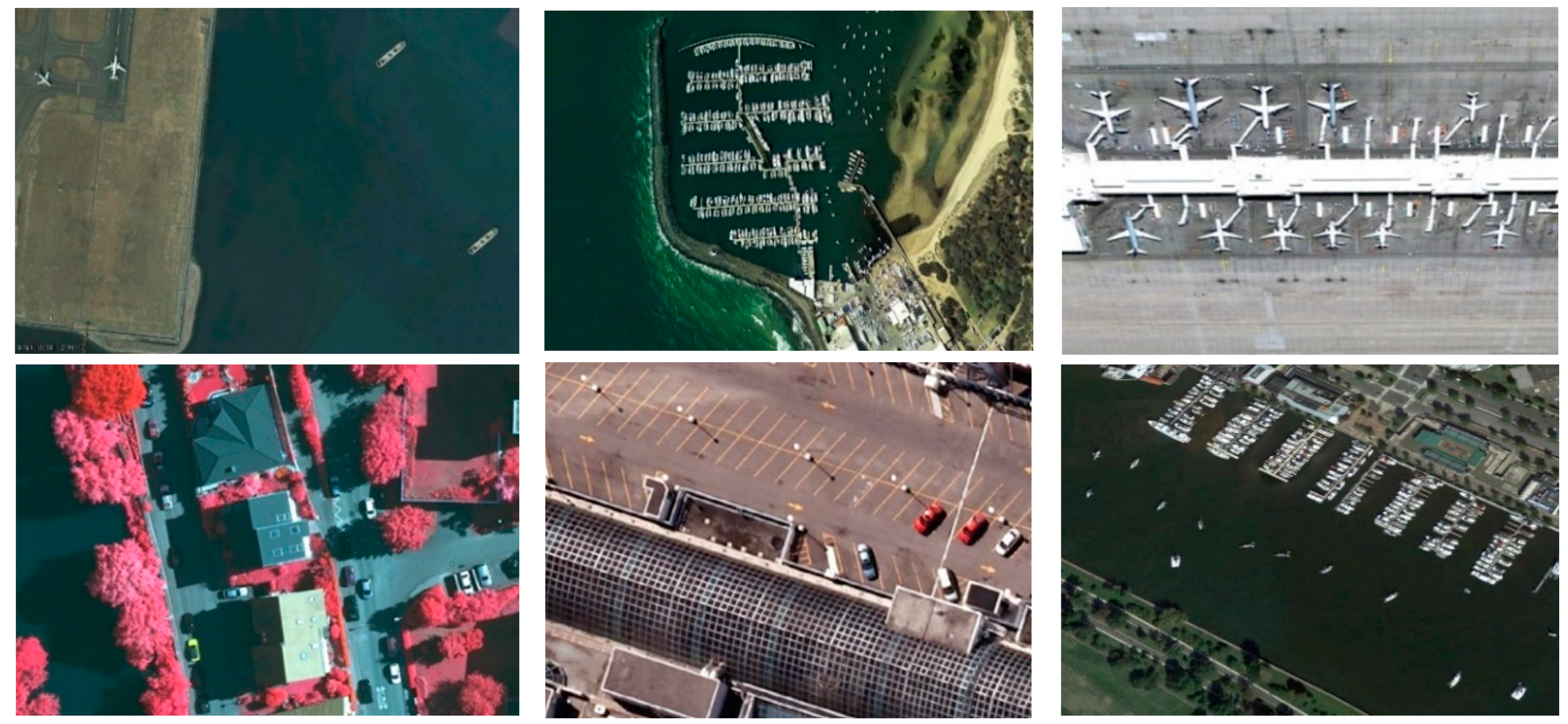
• In remote sensing images, each object does not have a fixed size and often appears at various scales. Further, the datasets mostly were collected from different resources with different resolutions.
• The remote sensing image is very large and contains a lot of small objects that sometimes appear in dense groups, such as vehicles and storage tanks. This adds significant challenges for geospatial object detection methods. By using normal object detection methods, the loss of small objects in RSI is very large, so there is an urgent need to optimize the detection methods.
• The aerial images are enormous and overcrowded with many kinds of small objects. Therefore, the manual annotation of objects is very complex and costly. Additionally, object detection in RSIs is a small sample setting problem. Although there are methods specifically designed for small sample setting problems, like rank-1 feedforward neural network (FNN) in [40], deep learning architectures are data hungry and thus, the training samples for object detection from RSIs are inadequate for training them.
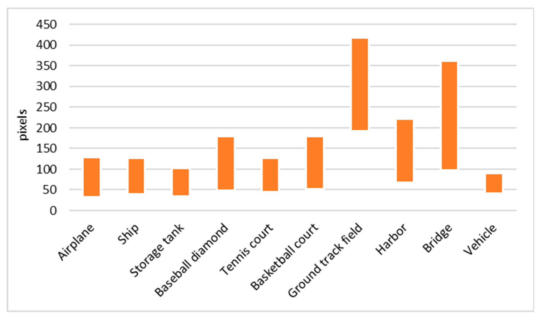
• The surrounding area of each different class is not the same as can be seen in Figure 1. For example, ships and airplanes mostly have a clear background and also have special colors and shapes that make them distinguishable. In contrast, many objects like vehicles and harbors do not have a special appearance or properties, so they need to be treated differently.

This paper deals with all of the above issues and difficulties. An effective deep CNN framework is introduced to detect multi-scale and multi-class objects in RSIs, and this framework has the ability to deal with these very large variabilities and challenges to fit the properties of the RSIs. Our framework is based on the region proposal: Its pipeline first generates the region proposals and then classifies each proposal into categories. The method of this framework is divided into two stages. The first stage is the feature extraction and the RPN. A shallow and deep CNN is constructed to extract features from each input image. These extracted features are designed to improve the resolution, reduce the loss of small objects and optimize the localization. Then, the output of shallow-deep feature extraction (SDFE) is fed into the RPN to extract multi-scale region proposals. In the RPN, to improve the accuracy, multi-scale anchor boxes with a specific CNN filter were used on multi-scale feature maps. After that, the outputs of these two networks are combined and fed into the second stage, which is fast R-CNN for the accurate detection of each object. Since RSIs have a large scale with the limitation of manual annotations, during the training, the horizontal flip is used. The main contributions of our framework are:

• A novel framework suitable for VHR remote sensing imagery was designed, which can detect the multi-scale and multi-class object in large-scale complex scenes.
• A feature pyramid extraction was designed which has a button-up pathway (BU), top-down pathway (TD) and many lateral connections to connect between the BU and TD layers to get higher semantic and resolution information to correspond with the situation of remote sensing images, which contain various sizes of objects.
• The feature map of each different layer was allocated to objects of specific scales, which increase the detection accuracy.
• The multiple feature maps produced were combined. Therefore, the resolution increased, and multiple levels of details could be considered simultaneously. Additionally, it is more accurate to detect various sizes of objects and densely packed objects.
• A shallow network was used which improves the localization and the time of performance (training and testing time).

The structure of the rest of this paper is given as follows. Section 2 describes the framework of the method in detail, the dataset description and evaluation metrics. An explanation of the results of the three different experiments and their comparisons are in Section 3. The conclusion and future work are given in Section 4.

2. Methods

The architecture of our approach is represented in Figure 2. It includes two stages, which depend on faster R-CNN. In the first stage, the feature extraction and the multi-scale RPN were used to extract the feature maps with high semantics information and the resolution was enhanced by using deeper and shallower networks. Additionally, a multi-scale and multi-filter (MS-MF) region proposal network was used. The operation of categorizing and locating each object is in the second stage. These two stages share the same multi-scale feature maps. These methods are introduced in detail.

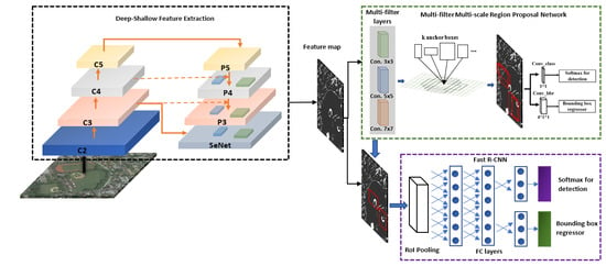
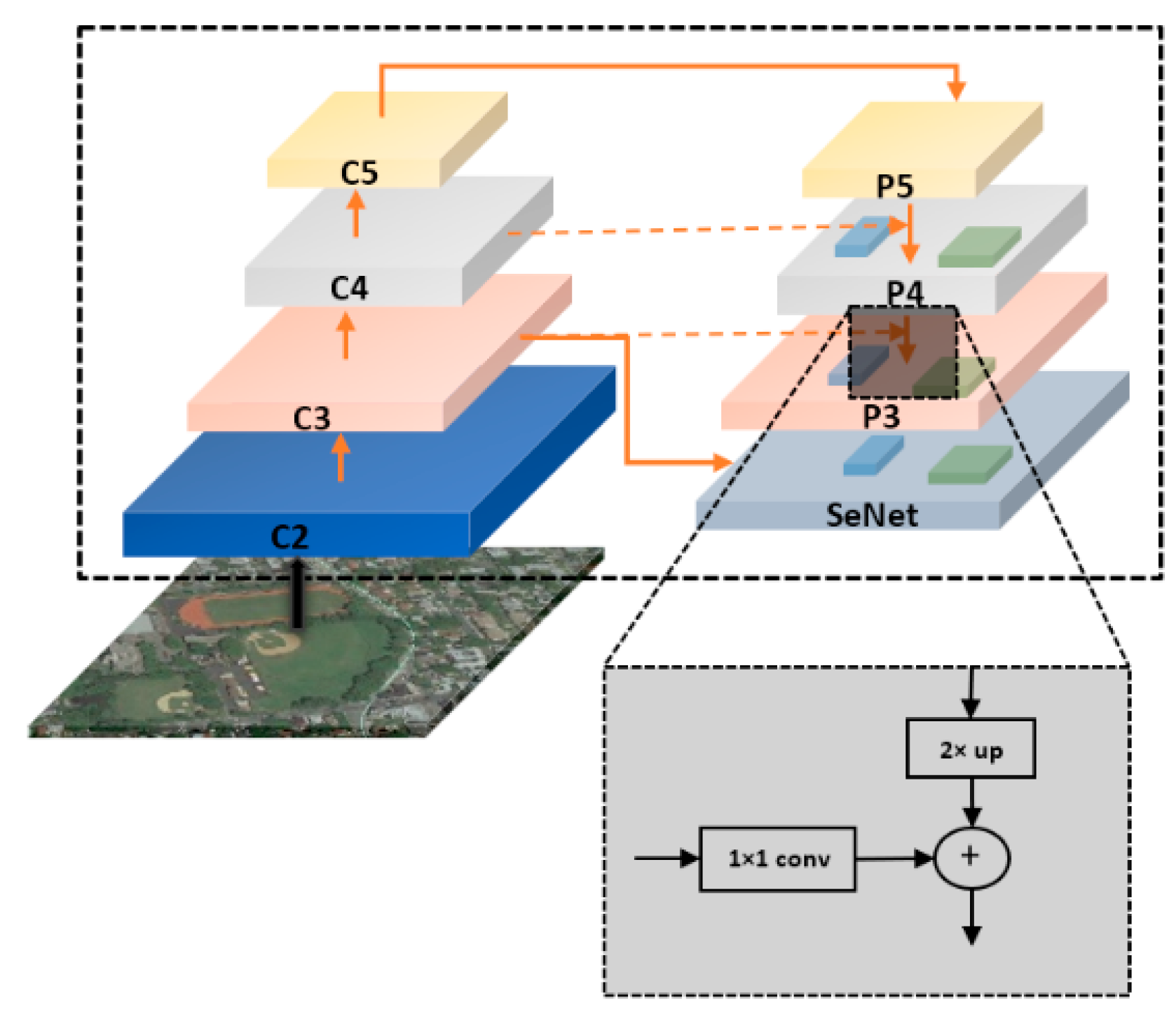
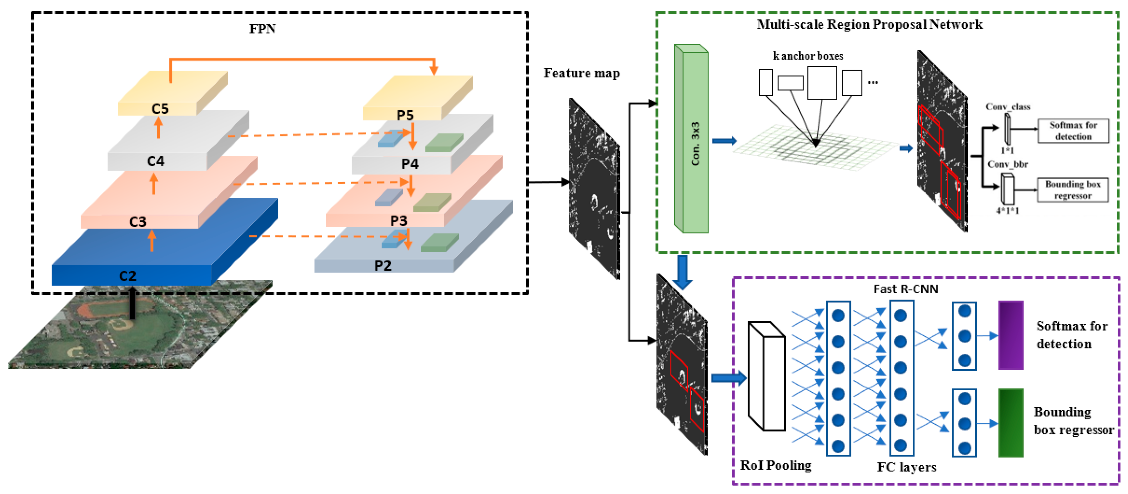
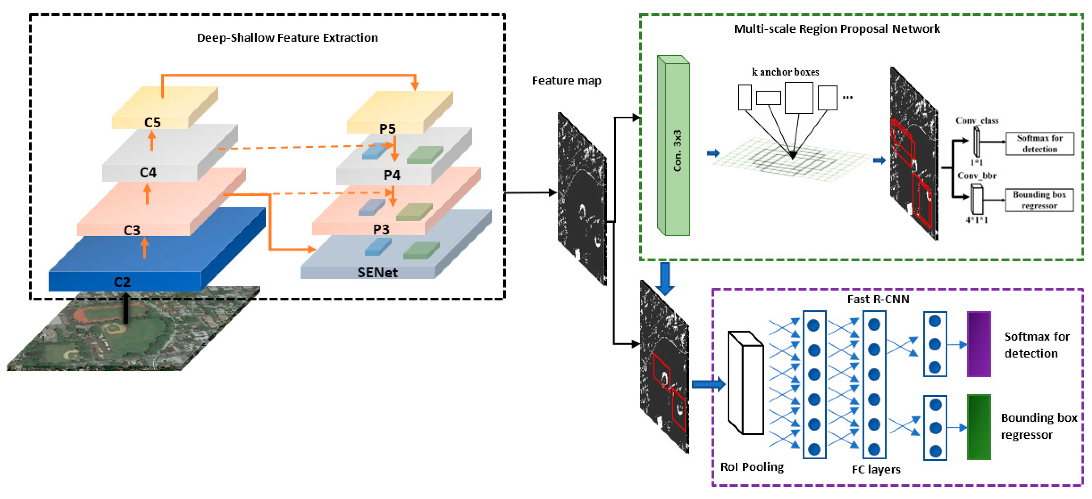
2.1. Shallow-Deep Feature Extraction Network (SDFE)

Designing the feature extractor is very important for enhancing the detection and performance operations. A very deep model needs a large amount of training samples, and there is a comparative scarcity of labeled RSIs as a dataset. Deeper models are also costly and lead to losing small objects. Based on the requirement to extract feature maps which capture large and small objects effectively, a shallow-deep network was designed to get feature maps that combine strong features and a low loss. As it is known, deep CNN is an efficient network to get stronger features and extract large objects. Shallow CNN is used to detect small objects, reduce the computational cost and improve localization.

The pyramid architecture of the feature extractor has been widely used in many studies. He et al. [23] introduced ResNet, which is an effective network to increase the accuracy of the deeper models. However, very deep models are not suitable for all kinds of data [16,41]. The principle advantage of hierarchical structures to extract features is that each level produces a multi-scale feature with strong semantics and achieves higher resolution. There are many different kinds of architectures for pyramid feature extractors [10,26], such as the feature image pyramid [42], single feature map, pyramidal feature hierarchy and FPN [26]. The first CNN pyramid hierarchy is SSD [27]. SSD reuses the multi-scale feature maps; these maps are computed from the forward-pass of different layers. As SSD does not reuse the high-resolution map of the lower layers of its hierarchy feature Figure 3a, SSD is not ideal to detect small objects. The last layer of the bottom-up feature map has higher semantic information, but the localization performance is poor [19,26,43]. In contrast, in the feature pyramid network [26], the features of the top-down pathway are enhanced by lateral connections, which merge the output of the bottom-up pathways with the top-down pathways. Each lateral connection merges feature maps of the same spatial level from these two different pathways. As a result, high resolution and strong segmentation is obtained at the same time. In this study, the idea of FPN with ResNet 101 as the BU network is adopted.

In their study, [23] proposed ResNet as a deeper and more effective framework, providing a solution for the problems of deeper networks, which are difficult to train due to the vanishing gradient problem. By using the deep residual learning framework, residual block, it can be assumed that $x$ is the input and the true output is $H(x)$, as shown in Figure 4. The residual is the difference between $x$ and $\mathscr{H}(x)$: $ℱ(x)≔\mathscr{H}(x)-x$. To get the original function, the equation was rearranged to be $\mathscr{H}(x)=ℱ(x)+x$. With this kind of shortcut connections, getting neither more parameters nor complex calculations, it is easy to use and combine ResNet with any kind of network. The equation of the ResNet building block is defined as:

$$Y=ℱ(X,\{W_i\})+X$$

(1)

where $Y,X$, and $W_i$ represent the output, input and the parameters of the $ith$ convolutional layers to be learned, respectively. $ℱ(X,\{W_i\})$ represents the residual mapping, which is already learned.

ResNet has various architectures: ResNet-50, ResNet-101 and ResNet-152. The number of each ResNet corresponds to how many residual network layers are used. In this study, ResNet-101 was used as the BU network to obtain a good balance between feature extraction and computing resources. The last blocks of Conv2, Conv3, Conv4 and Conv5, which are 3×3 convolutional kernels with {4, 8, 16, 32} strides, respectively, are named {C2, C3, C4, C5} as shown in Figure 2. To up-sample the TD feature maps, the element-wise was added to the corresponding BU map (lateral connection). Figure 5 shows the operation of merging layers. Finally, a 3×3 convolutional layer was added on each merged map to minimize the aliasing effect of the up-sampling operation and to get {P2, P3, P4, P5}, which are the final feature maps.

To carry out the requirements of the RSI situation, SENet [44] was added to the feature extraction to improve the performance and to combine the deep and shallow networks. The goal of SENet was to create a network that works to increase its sensitivity, as well as to keep and use the useful features and omit the others via two steps called squeeze and excitation, before feeding these features to the next operation. As shown in Figure 6, the first FC layer was followed by the ReLU function, adding the necessary nonlinearity. Its output channel complexity was also reduced by a certain ratio = 16, which gives a balance between the complexity and accuracy. The second FC was followed by a Sigmoid activation function, giving each channel a smooth output. With all these steps, adding a function to any model without additional computing costs can be achieved. SENet in our model was fed by the output of C3, then to another 3×3 convolutional.

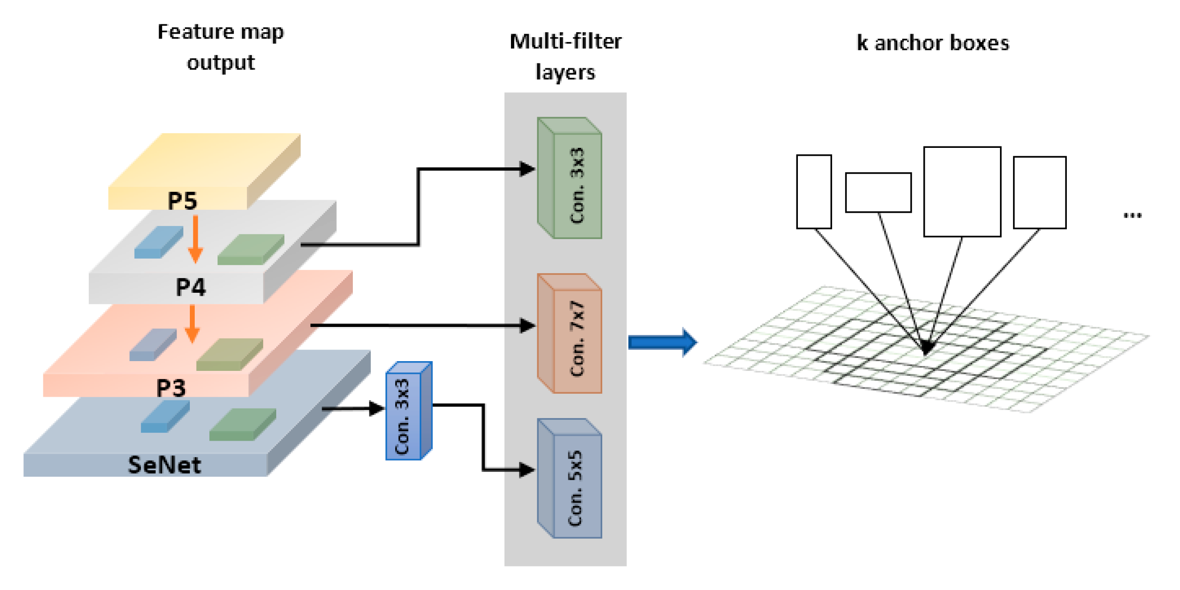
2.2. MS-MF Region Proposal Network

A good detector in geospatial object detection should have the ability to cover most objects and their various sizes. In [45], the authors broke down the R-CNN execution into several layers. In the anchor generation layer, a fixed number of anchors (bounding boxes) were generated. The number and shape of the anchors depend on the amount and values of scales and ratios. Then, in the region proposal layer, the operation of scoring each region proposal as a background or foreground class and obtaining corresponding bounding box regression coefficients occurred by using the 3×3 convolutional layer and was followed by two 1×1 convolutional layers. This study used a small network sliding over each feature map, i.e., the outputs of the P3, P4, SENet layers, with three types of convolution filter (kernel) layers (3×3, 5×5, 7×7). This is called a multi-filter (MF). The 5×5 convolution slides over SENet, 3×3 convolution slides over P4 and 7×7 convolution slides over P3, as shown in Figure 7. Each sliding window was mapped to a lower-dimensional feature (512 features). Each sliding window position has one anchor box $B_i=(b_i^x,b_i^y,b_i^w,b_i^h)$ predicted, where $b_i^x$ and $b_i^y$ are the top-left predicted region coordinates, and $b_i^w$ and $b_i^h$ are the width and the height, respectively.

In the RPN, this study used the same two different scales on each different layer of the feature map to catch as many objects as possible, see

Table 1. Training methods and what is used in each of them.

Performance Stages	Layers of Feature Map	Scales	Ratios	Filters
(a) All FPN + MS	P5, P4, P3, P2	The same two scales for each layer	[1, 0.5, 2, 1/3., 3., 1.5, 1/1.5]	-
(b) SD-MS	P4, P3, SENet	The same two scales for each layer	[1, 0.5, 2, 1/3., 3., 1.5, 1/1.5]	-
(c) SDFE + MS-MF, Figure 2	P4, P3, SENet	The same two scales for each layer	[1, 0.5, 2, 1/3., 3., 1.5, 1/1.5]	3 × 3, 5 × 5, 7 × 7 conv.

. In addition, because this study deals with a multi-category dataset (NWPU VHR-10), and this kind of dataset has images with different types of resolution and object shapes, these values were set [1, 0.5, 2, 1/3., 3., 1.5, 1/1.5] to the anchor ratios and [1.,0.12] to the anchor scales to create a multi-scale (MS) anchor over each feature map. Furthermore, the anchor assigned the object as a foreground sample if the threshold of intersection over union (IoU) ≥ 0.7, and as a background, if IoU < 0.3. In the second stage, the thresholds were 0.5 and 0, respectively. Finally, 256 was set to be the size of the mini-batch. The foreground boxes were selected by computing the IoU overlap of all the anchor boxes inside the input image with all ground-truth boxes, and those boxes were marked as foreground boxes if their maximum IoU overlaps with the ground-truth box or exceeds the value of the threshold. IoU was used to evaluate object detector performance. The formula for IoU is:

$$\mathrm{IoU}=\frac{\mathrm{area}(\mathrm{Bpb}\cap \mathrm{Bgt})}{\mathrm{area}(\mathrm{Bpb}\cup \mathrm{Bgt})}$$

(2)

where the area (Bpb ∩ Bgt) is the area of the overlap between the predicted bounding box and the ground-truth bounding box area, and area (Bpb ∪ Bgt) is the area of the union, which is the area surrounded by both the predicted bounding box and the ground-truth bounding box area.

To accelerate the operation of the RPN, only the highest score of 12,000 regression boxes was taken by the NMS operation [46,47] to get 2000 proposals. Alternatively, from 6000 regression boxes, 1000 proposals were taken in the test time, also by the NMS operation.

To calculate the loss of each detection layer in this stage, it was supposed that the combination of the loss values of the classification and bounding box regression [36] from the above equation can be defined as:

$$L(X,Y,B_{gt},B_{rb})=L_{cls}(p(X),Y)+\lambda [Y\ge 1]L_{bbr}(B_{gt},B_{rb})$$

(3)

where $L_{cls}(p(X),Y)=-\log p_y(X)$ is the log loss for true class Y (cross-entropy loss),

• X is the predicted probability anchor,
• $\lambda$ is the balancing parameter = 1,
• $[Y\ge 1]$ is used to evaluate to 1 when Y ≥ 1 and 0 otherwise,
• and $B_{rb}$ is the bounding box regression area.

We calculate the loss of the bounding box regression as the following:

$$L_{bbr}(B_{gt},B_{rb})=Smoot{h}_{L1}(x{B}_{gt}-B_{rb})$$

(4)

where

$$Smoot{h}_{L1}(x)=\{\begin{array}{lllll}0.5x^2,& & & & \left|x\right|<1\\ \left|x\right|-0.5,& & & & otherwise\end{array}$$

(5)

2.3. Object Detection Network

In the previous section, this study obtained the predicted region proposals. RoI pooling was used to extract the characteristics of each region proposal, and it was ideal to speed up the training and testing operations. Furthermore, RoI pooling can improve both the object classification and bounding box regression accuracy. The RPN, as was mentioned before in Section 2.2, was not essentially labeling the region box to its category. It is just used to determine if the predicted region proposal is either background or foreground (i.e., if the region proposal contains a target or not). Therefore, the benefit of the RoI pooling is to take all the output of the RPN and all feature vectors. These were cropped out from the SDFE by using array slicing, then they were resized to a fixed size with N strides [25], Figure 2. In this study, the RoI pooling layer was applied for each box with a fixed size (14, 14) and 2 strides. Then, it was followed by two FC layers with 1024 neurons. Finally, the output of these last two layers was fed to two separate FC layers. One of them was used to obtain the class label predictions and the other to obtain the bounding box location for each proposal. Moreover, NMS was used in the RPN and in this stage to reduce redundancy.

Here, the loss function is similar to the loss function of the RPN, but the difference is that the classification layer of the RPN deals with only two classes, the foreground and background and the last classification layer of this stage deals with all object classes [16,19].

3. Experiments

This study implemented and evaluated the model by using Keras and Tensorflow, and executed it on a PC with a Core i7-4790 CPU, NVIDIA GTX-1070 (8 GB memory), 8 GB RAM and the Windows 10 operating system.

3.1. Dataset Description

Cheng et al. in [15] proposed the NWPU VHR-10 dataset of 10 classes. This dataset is used in remote object detection to detect 10 classes. Its images were collected from two different sources with two different levels of resolution: 715 images were from Google Earth and 85 images from the Vaihingen dataset. This dataset has a separate folder containing all the ground-truth files of each image in the positive image set folder which has 650 images. Each image in this folder contains at least one object belonging to these 10 classes, and the other 150 images are in the negative image set folder without any target. Each ground-truth file has all bounding boxes information of all target objects. Bounding boxes were manually annotated. The format of each bounding box is (x1, y1), (x2, y2), where (x1, y1) represents the top-left coordinate of the bounding box and (x2, y2) represents the right-bottom coordinate of the bounding box. NWPU VHR-10 was chosen for the following reasons. First, it was collected from different resources with various resolutions. Second, it contains 10 different classes, including 124 bridges (B), 302 ships (S), 163 ground track fields (GTF), 757 airplanes (A), 390 baseball diamonds (BD), 524 tennis courts (TC), 150 basketball courts (BC), 655 storage tanks (ST), 224 harbors (H), and 477 vehicles (V). The other reason is that each class has a different size. At the same time, the same class has objects with a different size, color and appearance, as shown in Figure 8. All of that serves the purpose of this study, which is to build a model that has the ability to deal with all of these differences and challenges. In this paper, the dataset was divided into 80% for training (520 images) and 20% for testing (130 images). The network settings were an iteration of 30K, an initial learning rate of 1e-3, a momentum size of 0.9, and a weight decay of 0.0001. Additionally, during training, the horizontal flip was used.

3.2. Evaluation Metrics

To assess the performance of the object detection approach, measures such as the precision-recall curve (PRC) and average precision (AP) were widely used [11,15,48,49]. The PRC depends on the area of overlap between the ground-truth and detection. The precision computes the fraction of detections that are true positives (TP). A recall formula was used to measure the fraction of positives that were correctly identified. The AP and mean AP (mAP) were used to compute the average value of precision over different levels of recall. Therefore, a higher AP value corresponds to better performance.

$$Precision=\frac{TP}{TP+FP}$$

(6)

$$Recall=\frac{TP}{TP+FN}$$

(7)

The output is TP if the value of $IoU>0.5$ between the ground-truth bounding box and the predicted bounding box, which is obtained from Equation (2). Otherwise, it is false positive (FP). Furthermore, if numerous detections overlap with the same ground-truth bounding box, only one is measured as TP and the others as FP.

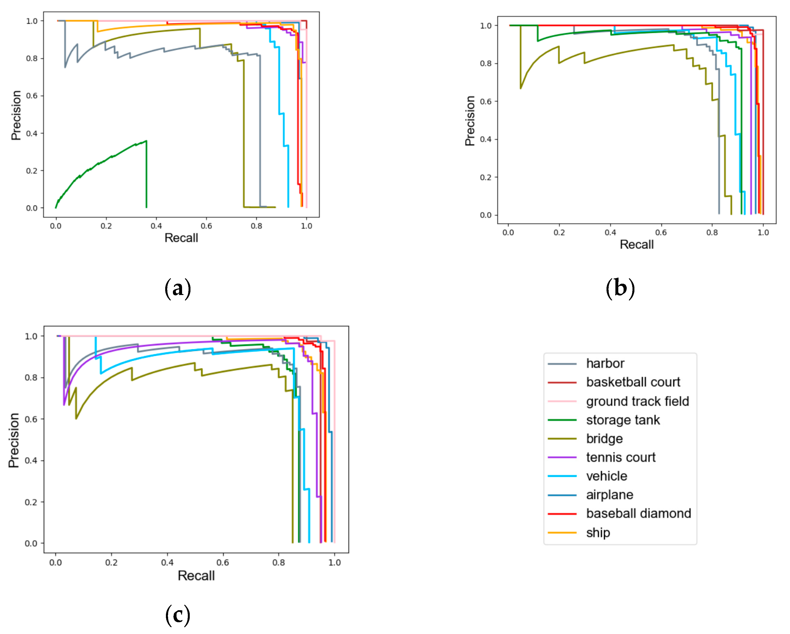
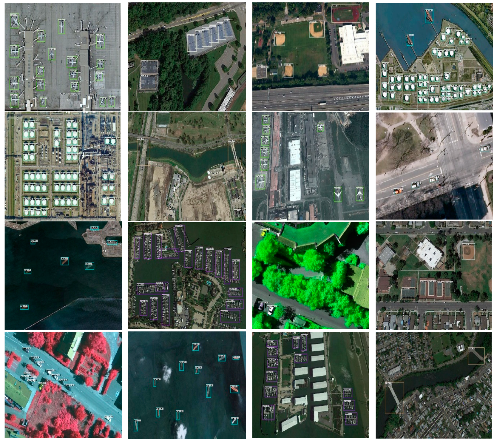
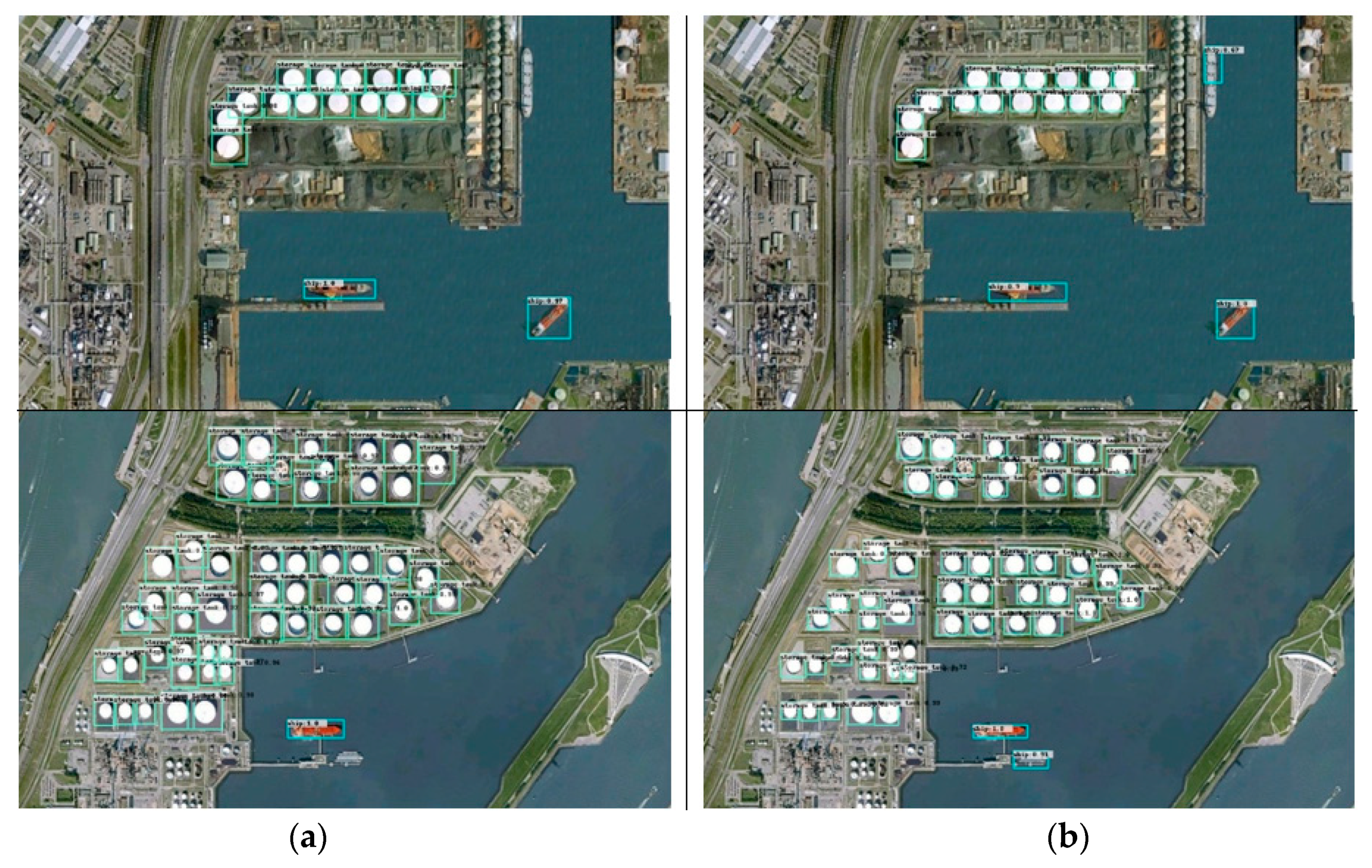
3.3. Experimental Results and Comparisons

This model was trained with three different architectures, as shown in Figure 2, Figure 9, Figure 10 and Table 1. In the first experiment, this study trained end-to-end all backbone layers of the feature extraction and the extracted anchor boxes by using the multi-scale (MS) sliding window over each feature map of [P5, P4, P3, P2] (FPN), Figure 9. For the second stage of the implementation, which is the shallow-deep feature extraction (SDFE), the P2 layer was removed and the output of C3 was connected with the SENet layer by lateral connection. Additionally, the output of P3 with the SENet layer was not combined. Thus, this method improves the quality of the feature extraction stage and increases localization performance. Furthermore, only feature maps of P3, P4 and the SENet were used. This study improved the time performance and detection accuracy. Similarly, in the last stage, the same multi-scale was used also in this experiment, as shown in Table 1b and Figure 10. Figure 2 is the architecture design of the third experiment. It is like the second experiment with only one addition, in which a different filter was added for each different feature map (MS-MF). The description of the structure is in Section 2.2. Table 1 and

Table 2. Comparisons of each experiment on the VHR-10 dataset, showing the components and results of mAP and recall for each experiment and the execution time of training and test.

Training Method	SDFE	MS	MF	mAP	Recall	Average Training Time per Image (Second)	Average Test Time per Image (Second)
All FPN + MS		√		83.31	89.46	1.2	3.3
SD-MS	√	√		91.55	94.39	0.9	2.5
SDFE + MS-MF	√	√	√	90.09	93.35	1.1	3

show the differences between all of these structures.

The results of these three different experiments are in

Table 3. The results of three experiments on the ten classes of the NWPU VHR-10 dataset.

Stages	FPN + MS		SD-MS		SDFE + MS-MF
	Recall	AP	Recall	AP	Recall	AP
A	98.02	97.60	97.03	96.98	99.01	98.36
S	97.92	96.54	98.96	97.31	96.88	95.07
ST	36.17	12.95	91.49	88.45	87.23	85.07
BD	98.29	95.69	98.29	97.62	96.58	96.05
TC	100.00	98.56	95.24	94.26	95.24	91.33
BC	100.00	100.00	100.00	99.76	95.00	94.87
GTF	100.00	99.89	100.00	99.65	100.00	99.88
H	83.95	71.14	82.72	80.37	87.65	82.54
B	87.50	70.75	87.50	73.72	85.00	73.78
V	92.73	90.01	92.73	87.35	90.91	83.96
Mean	89.46	83.31	94.39	91.55	93.35	90.09

. From this study and the results of the ten classes of NWPU VHR-10, very high accuracy detection was obtained, and from these different methods described above, the following were obtained: (1) For objects with a clear background, shape or that are not in dense groups such as airplanes and vehicles in this dataset, the first experiment with the deep feature extraction network gives very good results. (2) Alternatively, a shallow feature extraction network is the best choice to detect objects which are in dense groups, such as storage tanks and harbors. (3) Any object that has a large size with a clear shape obtained almost the same results in all experiments, like the ground track field, basketball court, tennis court and baseball diamond. (4) The last experiment with the multi-filter does not give a significant effect, but it gives evidence that a deep network is good to extract and detect the large size of an object, and small objects are probably lost using small filters. (5) Additionally, the third experiment was tested by applying a small filter on the SENet layer (3×3 conv.) and an unacceptable effect was obtained on the result: mAP was 87.03. This gives evidence that using small filters negatively affects small object detection and does not optimize the results. However, big filters improve the final results, especially for some targets, but they are not better than the second experiment (SD-MS) in general. In contrast, some results are good using different filters, such as airplanes, harbors and bridges, as can be seen in Table 3.

The following figures plot the PRCs of each experiment method among the testing classes. The recall ratio assesses the ability to detect more targets, whereas the precision assesses the performance of detecting correct objects rather than containing many false alarms. It can be observed from Figure 11 that the SD-MS obtains the best performance for all classes. It has also shown how the model is effective for extracting and detecting the different objects and obtains extremely high AP and recall values, as can be seen also in Table 3. The FPN+MS is not sufficiently balanced to deal with all of the various classes, especially with the storage tank class, as shown in Figure 11a. The SDFE + MS-MF improves the bridge detection more than the other approaches.

As discussed previously, our purpose was to detect multi-scale and multi-class objects in RSIs which have various resolutions, many small objects and dense groups. The SD-MS model detected objects of the ten classes of the test dataset. Figure 12 shows that this model (SD-MS) detected the objects effectively.

In addition, to quantitatively evaluate the proposed SD-MS model, this study compared it with eight existing methods: rotation-invariant CNN (RICNN) [15], region proposal networks with faster R-CNN (R-P-faster R-CNN) (R-P-F-R-CNN ) [50], deformable R-FCN (D-R-FCN) [51], collection of part detectors (COPD) [11], position-sensitive balancing (PSB) [20], deformable faster R-CNN (D-F-R-CNN) [52], recurrent detection with activated semantics (RDAS512) [53], and multi-scale CNN (MS-CNN) [19]. As can be seen from

Table 4. The AP values of eight object detections are compared with the two models, feature pyramid networks with multi-scale anchor (FPN+MS) and shallow-deep feature extraction with multi-scale anchor (SD-MS).

Class	RICNN	R-P-F-R-CNN	D-R-FCN	COPD	PSB	D-F-R-CNN	RDAS512	MS-CNN	FPN + MS	SD-MS
A	88.35	90.4	87.3	89.11	90.7	90.7	99.6	99.3	97.6	96.98
S	77.34	75	81.4	81.73	80.6	87.1	85.5	92	96.54	97.31
ST	85.27	44.4	63.6	97.32	80.3	70.5	89	83.2	12.95	88.45
BD	88.12	89.9	90.4	89.38	89.9	89.5	95	97.2	95.69	97.62
TC	40.83	79	81.6	73.27	75.5	89.3	89.6	90.8	98.56	94.26
BC	58.45	77.6	74.1	73.41	81.6	87.3	94.8	92.6	100	99.76
GTF	86.73	87.7	90.3	82.99	86.5	97.2	95.3	98.1	99.89	99.65
H	68.6	79.1	75.3	73.39	78.5	73.5	82.6	85.1	71.14	80.37
B	61.51	68.2	71.4	62.86	77.2	69.9	77.2	71.9	70.75	73.72
V	71.1	73.2	75.5	83.3	71	88.8	86.5	85.9	90.01	87.35
mAP	72.63	76.5	79.1	80.68	81.2	84.4	89.5	89.6	83.31	91.55

, the proposed SD-MS obtains the best mAP. It also indicates that our FPN with the MS method has the best results for the basketball court, tennis court, ground track field and vehicle classes. The best results of the ship and baseball diamond classes are obtained by SD-MS. This means that our model has had significant success in extracting and detecting the different objects. In contrast, RDAS512 is only 2% better than our FPN with MS to detect airplane objects. SD-MS is only 3.48% less than the PSB and RDAS512 methods for only bridge detection. Finally, COPD is the best model for only one object: a storage tank. As a result, the proposed SD-MS framework outperforms all comparison approaches for all ten classes of the NWPU VHR-10 dataset, which demonstrates the superiority of the proposed method compared with the eight other methods.

When the model was tested in each different experiment, it was noted that in many cases, the model of the first experiment (FPN+ MS) detected targets by drawing their bounding boxes but the value of AP was very low. For this reason, the first and the second models were tested with three different IoU evaluations (0.3, 0.4, 0.5).

Table 5. (a) is the results of the FPN+MS experiments using three different IoU values, getting big differences of results for each different IoU. The total effect is only from 4.91% to 11.42%. (b) is the results of the SD-MS experiments, and the effect of IoU is very weak. The total effect is only from 2.1% to 3.64%.

(a)				(b)
Class	0.3	0.4	0.5	0.3	0.4	0.5
A	98.71	97.60	97.60	98.00	98.00	96.98
S	98.50	98.50	96.54	97.31	97.31	97.31
ST	92.59	42.90	12.95	99.52	96.29	88.45
BD	95.69	95.69	95.69	98.47	98.47	97.62
TC	98.56	98.56	98.56	94.26	94.26	94.26
BC	100.00	100.00	100.00	99.76	99.76	99.76
GTF	99.89	99.89	99.89	99.65	99.65	99.65
H	89.20	85.51	71.14	90.52	86.78	80.37
B	84.11	73.54	70.75	86.17	78.61	73.72
V	90.01	90.01	90.01	88.22	87.35	87.35
mAP	94.73	88.22	83.31	95.19	93.65	91.55

shows that in the first experiment, the storage tank class experienced a big effect. Its AP changed from 12.95 to 92.59. The AP of the harbor class changed from 71.14 to 89.20, and the AP of the bridge class changed from 70.75 to 84.11. These three classes were affected strongly, but the other classes did not have a notable change. In contrast, the change of AP values with the SD-MS model is very low. The AP of the storage tank class only changed from 88.45 to 99.52. Additionally, the harbor class and bridge class did not experience a big change, as shown in Table 5. Most of the 10 classes did not experience any effect by changing IoU evaluations. The mAP only changed by 3.64%, which means that the SD-MS model effectively detected the different classes and obtained the goal of RSI object detection. As shown in Figure 13, the two models detect the storage tank perfectly, but the difference is that the bounding box of SD-MS is smaller and surrounded the object more perfectly than the FPN+MS model. For that reason, the mAP of SD-MS is higher.

Based on the above results and comparisons, the SD-MS model deals with most of the difficulties and challenges of RSIs. Each class has its situation and difficulties. Vehicles, ships and airplanes are small objects and sometimes appear in very complex environments. Storage tanks are small and are often in dense groups. Baseball diamonds, basketball courts, tennis courts and ground track fields appear in different sizes and colors. Shallow and deep feature extraction with multi-scale anchor boxes was used, which offered many benefits for extracting more objects and reducing the loss. Its accuracy is extremely high and has the ability to detect most of these various objects and their situations and is not affected by IoU evaluations change. In contrast, the performance time of the proposed model is long for many reasons:

• As known, VHR images take a long time for processing.
• The CPU of the device is very slow and the RAM of the GPU and of the device are both small, only 8 GB. These were important factors that slowed down processing.
• The structure of SDFE makes the process work in a straight line, happening one after the other in a series from C1 to P2. This also slows down the speed of the feature extraction. Therefore, a good way to improve the speed is by having the feature extraction structures work in parallel.

4. Conclusions

In this paper, a unique shallow-deep feature extraction framework with a multi-scale anchor size was proposed to enhance detection of the remote sensing images. The feature extractor was redesigned by combining the deep and shallow CNN based on ResNet-101 and SENet to enhance the feature extraction. After that, a different multi-scale anchor was played over each level of the feature map to improve the cropping of each different object. The experiments of our model with the NWPU VHR-10 dataset show the following: (1) Our model has the ability to extract the different object categories. (2) Our model shows the best detection for dense groups and small objects. (3) A very effective feature extraction was provided, beating most RSIs challenges. (4) By using three different stages of the experiment, this study demonstrated various factors that affect the detection. (5) The AP values of the SD-MS model do not change if the evaluation of IoU is changed, which means its accuracy is exceptionally high and does not have many false detections. (6) Our model obtained the best AP when it was compared with the eight state-of-the-art methods. In future work, the authors will focus on improving the time of the performance and feature extraction. Additionally, focus will be placed on enhancing the IoU operation to optimize the cropping of each object.

References

1. Zou, Z.; Shi, Z.; Guo, Y.; Ye, J. Object Detection in 20 Years: A Survey. arXiv 2019, arXiv:1905.05055v1. [Google Scholar]
2. Zhu, C.; Zhou, H.; Wang, R.; Guo, J. A Novel Hierarchical Method of Ship Detection from Spaceborne Optical Image Based on Shape and Texture Features. IEEE Trans. Geosci. Remote Sens. 2010, 48, 3446–3456. [Google Scholar] [CrossRef]
3. Qi, S.; Ma, J.; Lin, J.; Li, Y.; Tian, J. Unsupervised Ship Detection Based on Saliency and S-HOG Descriptor from Optical Satellite Images. IEEE Geosci. Remote Sens. Lett. 2015, 12, 1451–1455. [Google Scholar]
4. Han, J.; Zhou, P.; Zhang, D.; Cheng, G.; Guo, L.; Liu, Z.; Bu, S.; Wu, J. Efficient, simultaneous detection of multi-class geospatial targets based on visual saliency modeling and discriminative learning of sparse coding. ISPRS J. Photogramm. Remote Sens. 2014, 89, 37–48. [Google Scholar] [CrossRef]
5. Han, J.; Zhang, D.; Cheng, G.; Guo, L.; Ren, J. Object Detection in Optical Remote Sensing Images Based on Weakly Supervised Learning and High-Level Feature Learning. IEEE Trans. Geosci. Remote Sens. 2015, 6, 53. [Google Scholar] [CrossRef]
6. Shi, Z.; Yu, X.; Jiang, Z.; Li, B. Ship Detection in High-Resolution Optical Imagery Based on Anomaly Detector and Local Shape Feature. IEEE Trans. Geosci. Remote Sens. 2014, 52, 4511–4523. [Google Scholar]
7. Tang, J.; Deng, C.; Huang, G.-B.; Zhao, B. Compressed-Domain Ship Detection on Spaceborne Optical Image Using Deep Neural Network and Extreme Learning Machine. IEEE Trans. Geosci. Remote Sens. 2015, 53, 1174–1185. [Google Scholar] [CrossRef]
8. Viola, P.; Jones, M. Rapid object detection using a boosted cascade of simple features. IEEE Comput. Soc. Conf. Comput. Vis. Pattern Recognit. 2001, 1, 511–518. [Google Scholar]
9. Dalal, N.; Triggs, B. Histograms of oriented gradients for human detection. In Proceedings of the 2005 IEEE Computer Society Conference on Computer Vision and Pattern Recognition (CVPR’05), San Diego, CA, USA, 20–26 June 2005; Volume 1, pp. 886–893. [Google Scholar]
10. Zhao, Z.; Zheng, P.; Xu, S.; Wu, X. Object Detection with Deep Learning: A Review. IEEE Trans. Neural Netw. Learn. Syst. 2019, 1–21. [Google Scholar] [CrossRef]
11. Cheng, G.; Han, J.; Zhou, P.; Guo, L. Multi-class geospatial object detection and geographic image classification based on collection of part detectors. ISPRS J. Photogramm. Remote Sens. 2014, 98, 119–132. [Google Scholar] [CrossRef]
12. Wan, L.; Zheng, L.; Huo, H.; Fang, T. Affine Invariant Description and Large-Margin Dimensionality Reduction for Target Detection in Optical Remote Sensing Images. IEEE Geosci. Remote Sens. Lett. 2017, 14, 1116–1120. [Google Scholar] [CrossRef]
13. Yuan, Y.; Hu, X. Bag-of-Words and Object-Based Classification for Cloud Extraction from Satellite Imagery. IEEE J. Sel. Top. Appl. Earth Obs. Remote Sens. 2015, 8, 4197–4205. [Google Scholar] [CrossRef]
14. Zhang, F.; Du, B.; Zhang, L.; Xu, M. Weakly Supervised Learning Based on Coupled Convolutional Neural Networks for Aircraft Detection. IEEE Trans. Geosci. Remote Sens. 2016, 54, 5553–5563. [Google Scholar] [CrossRef]
15. Cheng, G.; Zhou, P.; Han, J. Learning Rotation-Invariant Convolutional Neural Networks for Object Detection in VHR Optical Remote Sensing Images. IEEE Trans. Geosci. Remote Sens. 2016, 54, 7405–7415. [Google Scholar] [CrossRef]
16. Deng, Z.; Sun, H.; Zhou, S.; Zhao, J.; Lei, L.; Zou, H. Multi-scale object detection in remote sensing imagery with convolutional neural networks. ISPRS J. Photogramm. Remote Sens. 2018, 145, 3–22. [Google Scholar] [CrossRef]
17. Kim, K.-H.; Hong, S.; Roh, B.; Cheon, Y.; Park, M. PVANET: Deep but Lightweight Neural Networks for Real-time Object Detection. arXiv 2016, arXiv:1608.08021. [Google Scholar]
18. Hong, S.; Roh, B.; Kim, K.-H.; Cheon, Y.; Park, M. PVANet: Lightweight Deep Neural Networks for Real-time Object Detection. arXiv 2016, arXiv:1611.08588. [Google Scholar]
19. Guo, W.; Yang, W.; Zhang, H.; Hua, G. Geospatial Object Detection in High Resolution Satellite Images Based on Multi-Scale Convolutional Neural Network. Remote Sens. 2018, 10, 131. [Google Scholar] [CrossRef]
20. Zhong, Y.; Han, X.; Zhang, L. Multi-class geospatial object detection based on a position-sensitive balancing framework for high spatial resolution remote sensing imagery. ISPRS J. Photogramm. Remote Sens. 2018, 138, 281–294. [Google Scholar] [CrossRef]
21. He, K.; Gkioxari, G.; Dollár, P.; Girshick, R. Mask R-CNN. In Proceedings of the IEEE International Conference on Computer Vision (ICCV), Venice, Italy, 22–29 October 2017; pp. 2980–2988. [Google Scholar]
22. Krizhevsky, A.; Sutskever, I.; Hinton, G.E. ImageNet Classification with Deep Convolutional Neural Networks. In Proceedings of the Advances in Neural Information, Lake Tahoe, NV, USA, 3–6 December 2012; pp. 1097–1105. [Google Scholar]
23. He, K.; Zhang, X.; Ren, S.; Sun, J. Deep Residual Learning for Image Recognition. In Proceedings of the 2016 IEEE Conference on Computer Vision and Pattern Recognition (CVPR), Las Vegas, NV, USA, 26 June–1 July 2016; pp. 770–778. [Google Scholar]
24. Dai, J.; Li, Y.; He, K.; Sun, J. R-FCN: Object Detection via Region-based Fully Convolutional Networks. arXiv 2016, arXiv:1605.06409v1. [Google Scholar]
25. Ren, S.; He, K.; Girshick, R.; Sun, J. Faster R-CNN: Towards Real-Time Object Detection with Region Proposal Networks. IEEE Trans. Pattern Anal. Mach. Intell. 2017, 39, 1137–1149. [Google Scholar] [CrossRef] [PubMed] [Green Version]
26. Lin, T.-Y.; Dollár, P.; Girshick, R.; He, K.; Hariharan, B.; Belongie, S. Feature Pyramid Networks for Object Detection. arXiv 2017, arXiv:1612.03144. [Google Scholar]
27. Wei Liu, D.A.; Erhan, D.; Szegedy, C.; Reed, S.; Fu, C.-Y.; Berg, A.C. SSD: Single Shot MultiBox Detector. Proc. Eur. Conf. Comput. Vis. 2016, 2016, 21–37. [Google Scholar]
28. Redmon, J.; Divvala, S.; Girshick, R.; Farhadi, A. You Only Look Once: Unified, Real-Time Object Detection. In Proceedings of the IEEE Conference on Computer Vision and Pattern Recognition (CVPR), Las Vegas, NV, USA, 27–30 June 2016; pp. 779–788. [Google Scholar]
29. Shen, Z.; Liu, Z.; Li, J.; Jiang, Y.-G.; Chen, Y.; Xue, X. DSOD: Learning Deeply Supervised Object Detectors from Scratch. arXiv 2018, arXiv:1708.01241. [Google Scholar]
30. Girshick, R.; Donahue, J.; Darrell, T.; Malik, J. Region-Based Convolutional Networks for Accurate Object Detection and Segmentation. IEEE Trans. Pattern Anal. Mach. Intell. 2016, 38, 142–158. [Google Scholar] [CrossRef] [PubMed]
31. Uijlings, J.R.R.; Van De Sande, K.E.; Gevers, T.; Smeulders, A.W.M. Selective Search for Object Recognition. Int. J. Comput. Vis. 2013, 104, 154–171. [Google Scholar] [CrossRef] [Green Version]
32. Cortes, C.; Vapnik, V. Support vector machine. Mach. Learn. 1995, 20, 273–297. [Google Scholar] [CrossRef]
33. He, K.; Zhang, X.; Ren, S.; Sun, J. Spatial Pyramid Pooling in Deep Convolutional Networks for Visual Recognition. IEEE Trans. Pattern Anal. Mach. Intell. 2015, 37, 1904–1916. [Google Scholar] [CrossRef] [Green Version]
34. Lazebnik, S.; Schmid, C.; Ponce, J. Beyond Bags of Features: Spatial Pyramid Matching for Recognizing Natural Scene Categories. In Proceedings of the IEEE Computer Society Conference on Computer Vision and Pattern Recognition (CVPR’06), New York, NY, USA, 17–22 June 2006; pp. 2169–2178. [Google Scholar]
35. Perronnin, F.; Sánchez, J.; Mensink, T. Improving the Fisher Kernel for Large-Scale Image Classification. In European Conference on Computer Vision; Springer: Berlin/Heidelberg, Germany, 2010; pp. 143–156. [Google Scholar] [Green Version]
36. Girshick, R. Fast R-CNN. In Proceedings of the 2015 IEEE International Conference on Computer Vision (ICCV), Santiago, Chile, 7–13 December 2015; pp. 1440–1448. [Google Scholar]
37. Roy, A.G.; Navab, N.; Wachinger, C. Recalibrating Fully Convolutional Networks with Spatial and Channel “Squeeze and Excitation” Blocks. IEEE Trans. Med. Imaging 2019, 38, 540–549. [Google Scholar] [CrossRef]
38. Lin, Z.; Ji, K.; Leng, X.; Kuang, G. Squeeze and Excitation Rank Faster R-CNN for Ship Detection in SAR Images. IEEE Geosci. Remote Sens. Lett. 2019, 16, 751–755. [Google Scholar] [CrossRef]
39. Liu, F.; Chen, C.; Gu, D.; Zheng, J. FTPN: Scene Text Detection with Feature Pyramid Based Text Proposal Network. IEEE Access 2019, 7, 44219–44228. [Google Scholar] [CrossRef]
40. Makantasis, K.; Doulamis, A.D.; Doulamis, N.D.; Nikitakis, A. Tensor-Based Classification Models for Hyperspectral Data Analysis. IEEE Trans. Geosci. Remote Sens. 2018, 56, 6884–6898. [Google Scholar] [CrossRef]
41. Yang, X.; Fu, K.; Sun, H.; Yang, J.; Guo, Z.; Yan, M.; Zhang, T.; Xian, S. R2CNN++: Multi-Dimensional Attention Based Rotation Invariant Detector with Robust Anchor Strategy. arXiv 2018, arXiv:1811.07126. [Google Scholar]
42. Felzenszwalb, P.F.; Girshick, R.B.; McAllester, D.; Ramanan, D. Object Detection with Discriminatively Trained Part-Based Models. IEEE Trans. Pattern Anal. Mach. Intell. 2010, 32, 1627–1645. [Google Scholar] [CrossRef]
43. Kong, T.; Sun, F.; Yao, A.; Liu, H.; Lu, M.; Chen, Y. RON: Reverse Connection with Objectness Prior Networks for Object Detection. In Proceedings of the IEEE Conference on Computer Vision and Pattern Recognition (CVPR), Honolulu, HI, USA, 21–26 July 2017; pp. 5244–5252. [Google Scholar]
44. Hu, J.; Shen, L.; Albanie, S.; Sun, G.; Wu, E. Squeeze-and-Excitation Networks. IEEE Trans. Pattern Anal. Mach. Intell. 2019. [Google Scholar] [CrossRef]
45. Girshick, R.; Donahue, J.; Darrell, T.; Malik, J. Rich Feature Hierarchies for Accurate Object Detection and Semantic Segmentation. In Proceedings of the IEEE Conference on Computer Vision and Pattern Recognition, Columbus, OH, USA, 23–28 June 2014; pp. 580–587. [Google Scholar]
46. Neubeck, A.; Gool, L.V. Efficient Non-Maximum Suppression. In Proceedings of the International Conference on Pattern Recognition (ICPR’06), Hong Kong, China, 20–24 August 2006; pp. 850–855. [Google Scholar]
47. Wan, L.; Eigen, D.; Fergus, R. End-to-end integration of a Convolutional Network, Deformable Parts Model and non-maximum suppression. In Proceedings of the IEEE Conference on Computer Vision and Pattern Recognition (CVPR), Boston, MA, USA, 7–12 June 2015; pp. 851–859. [Google Scholar]
48. Han, J.; Zhang, D.; Cheng, G.; Liu, N.; Xu, D. Advanced Deep-Learning Techniques for Salient and Category-Specific Object Detection: A Survey. IEEE Signal Process. Mag. 2018, 35, 84–100. [Google Scholar] [CrossRef]
49. Cheng, G.; Han, J. A survey on object detection in optical remote sensing images. ISPRS J. Photogramm. Remote Sens. 2016, 117, 11–28. [Google Scholar] [CrossRef] [Green Version]
50. Han, X.; Zhong, Y.; Zhang, L. An Efficient and Robust Integrated Geospatial Object Detection Framework for High Spatial Resolution Remote Sensing Imagery. Remote Sens. 2017, 9, 666. [Google Scholar] [CrossRef]
51. Xu, Z.; Xu, X.; Wang, L.; Yang, R.; Pu, F. Deformable ConvNet with Aspect Ratio Constrained NMS for Object Detection in Remote Sensing Imagery. Remote Sens. 2017, 9, 1312. [Google Scholar] [CrossRef]
52. Ren, Y.; Zhu, C.; Xiao, S. Deformable Faster R-CNN with Aggregating Multi-Layer Features for Partially Occluded Object Detection in Optical Remote Sensing Images. Remote Sens. 2018, 10, 1470. [Google Scholar] [CrossRef]
53. Chen, S.; Zhan, R.; Zhang, J. Geospatial Object Detection in Remote Sensing Imagery Based on Multiscale Single-Shot Detector with Activated Semantics. Remote Sens. 2018, 10, 820. [Google Scholar] [CrossRef]
Figure 1. Objects often have very different appearances and scales, and sometimes appear with a very complicated surrounding area in remote sensing images.
Remotesensing 11 02525 g001
Figure 2. Shallow-deep feature extraction with the multi-filter multi-scale region proposal network (RPN) architecture.
Remotesensing 11 02525 g002
Figure 3. (a) Visualization of the feature pyramid of single shot multibox detector (SSD) and its prediction operation, (b) visualization of the architecture of feature pyramid networks (FPN) (adapted from [26]).
Remotesensing 11 02525 g003
Figure 4. Visualization of the residual block of the residual network (ResNet).
Remotesensing 11 02525 g004
Figure 5. Lateral connection architecture and the way of merging the layers by the addition operation.
Remotesensing 11 02525 g005
Figure 6. Architecture of the original inception module (left) and the SE-inception module (right).
Remotesensing 11 02525 g006
Figure 7. Multi-filter multi-scale region proposal network (RPN) architecture.
Remotesensing 11 02525 g007
Figure 8. Object sizes of each class in the NWPU VHR-10 dataset.
Remotesensing 11 02525 g008
Figure 9. Feature pyramid networks (FPN) is feature extraction with multi-scale region proposal network (RPN) and is the architecture of the first training experiment.
Remotesensing 11 02525 g009
Figure 10. The architecture of the second stage of performance, using shallow-deep feature extraction with multi-scale region proposal network (RPN), (SD-MS).
Remotesensing 11 02525 g010
Figure 11. (a) The average precision (AP) values of the ten classes of the NWPU VHR-10 dataset obtained by the feature pyramid network (FPN) with the MS method (the first experiment). (b) The AP values of the ten classes of the NWPU VHR-10 dataset obtained by the SD-MS model (the second experiment). (c) The AP values of the ten classes of the NWPU VHR-10 dataset obtained by our shallow-deep feature extraction (SDFE) with MS-MF model (the third experiment).
Remotesensing 11 02525 g011
Figure 12. Detection results of our model SD-MS, which used ten classes of the NWPU VHR-10 dataset to test the results.
Remotesensing 11 02525 g012
Figure 13. (a) The results of the feature pyramid networks with multi-scale anchor (FPN+MS) experimentation by using three different threshold values of the intersection over union (IoU). The bounding box is larger than its target, which strongly influenced the accuracy of the measurement AP. (b) The detection results of the shallow-deep feature extraction with multi-scale anchor (SD-MS) model for the storage tank class. Each detected bounding box of each target is very close. This has a positive impact on the accuracy.
Remotesensing 11 02525 g013