Automated Extraction of Antarctic Glacier and Ice Shelf Fronts from Sentinel-1 Imagery Using Deep Learning

Abstract

Sea level rise contribution from the Antarctic ice sheet is influenced by changes in glacier and ice shelf front position. Still, little is known about seasonal glacier and ice shelf front fluctuations as the manual delineation of calving fronts from remote sensing imagery is very time-consuming. The major challenge of automatic calving front extraction is the low contrast between floating glacier and ice shelf fronts and the surrounding sea ice. Additionally, in previous decades, remote sensing imagery over the often cloud-covered Antarctic coastline was limited. Nowadays, an abundance of Sentinel-1 imagery over the Antarctic coastline exists and could be used for tracking glacier and ice shelf front movement. To exploit the available Sentinel-1 data, we developed a processing chain allowing automatic extraction of the Antarctic coastline from Seninel-1 imagery and the creation of dense time series to assess calving front change. The core of the proposed workflow is a modified version of the deep learning architecture U-Net. This convolutional neural network (CNN) performs a semantic segmentation on dual-pol Sentinel-1 data and the Antarctic TanDEM-X digital elevation model (DEM). The proposed method is tested for four training and test areas along the Antarctic coastline. The automatically extracted fronts deviate on average 78 m in training and 108 m test areas. Spatial and temporal transferability is demonstrated on an automatically extracted 15-month time series along the Getz Ice Shelf. Between May 2017 and July 2018, the fronts along the Getz Ice Shelf show mostly an advancing tendency with the fastest moving front of DeVicq Glacier with 726 ± 20 m/yr.

1. Introduction

The coastline of the Antarctic continent consists not only of solid rock but also dynamic glacier and ice shelf fronts. Iceberg calving and recent disintegration events of ice shelves make the Antarctic coastline a constantly changing boundary between land ice and ocean. Ice shelf and glacier fronts are sensitive indicators for glaciological processes and play an important role for ice sheet dynamics and mass balance. Changes in ice front position can influence ice sheet discharge as retreating fronts may enhance ice sheet flow through reduced buttressing effects [1]. If we want to understand the sea level rise contribution of Antarctica, besides many other parameters, current calving front dynamics have to be tracked. Only in this way, recent changes in glacier and ice shelf front movement can be detected. Additionally, our understanding of forces controlling calving front location (CFL) change is still limited as continuous Antarctic coastal-change time series are scarce [2]. This is attributed to the lack of suitable amounts of remote sensing imagery and the time-consuming manual delineation of calving fronts. But since the launch of Sentinel-1 year-round, medium-resolution and weather independent imagery over the Antarctic coastline with weekly revisit times is available. To exploit this abundance of data, a novel automatic approach for coastline extraction is needed to continuously track glacier and ice front fluctuations. But, so far, no automatic method exists to track dynamic glacier and ice shelf front change intra-annually.

Automatic coastline extraction from SAR (Synthetic Aperture Radar) imagery has been a challenging task for several decades [3]. Speckle and wind roughed sea lower the intensity contrast between sea and land and other object boundaries may have higher contrast than the actual coastline [4,5,6]. For the Antarctic coastline and polar coastlines in general, additional difficulties arise. The Antarctic coastline is defined as the boundary between the ice sheet (including floating ice shelves and glacier tongues) and the ocean [7]. In many cases, the Antarctic coastline can be difficult to detect on remote sensing imagery. For example, fast ice is fastened to the ice sheet, has similar backscatter values as the ice shelf surface but has originally developed from sea ice. Additionally, icebergs enclosed by slushy sea ice reduce the contrast between sea ice and the glacier tongue which makes the delineation more difficult. Therefore, most general image processing techniques like segmentation and edge detection don’t perform accurate enough [8]. Besides edge detection, classification-based approaches are used to extract the coastline, sometimes additionally with active contours [6,9,10,11,12]. For polar regions, classification approaches on SAR imagery are difficult to apply as backscatter varies exceptionally over the same spot throughout the year. Seasonal changes in sea ice and snow properties and melt modify backscatter characteristics over the ocean and ice sheet [13,14,15,16]. For example, the higher parts of the ice sheet may have the same backscatter intensity as open water and ice mélange scatters similar to a rough glacier surface.

Despite the many challenges that have to be faced to extract polar coastlines from SAR imagery, a few (semi-)automated approaches exist. Sohn and Jezek 1999 [15] applied the Roberts operator for edge extraction after edge enhancement and local thresholding for the Jacobshavn Glacier in Greenland based on ERS-1 imagery. They extracted the calving front of Jacobshavn Glacier with an accuracy of 2–3 pixels (200–300 m) for the year 1992. Liu and Jezek 2004 [4,8] developed an image processing chain for the RADARSAT mosaic from 1997 (later on also for 2000). After speckle reduction and edge enhancement, the image is segmented by using local adaptive thresholding. In the post-processing step, the Antarctic coastline is extracted by the canny edge detector. Errors occur in areas with wind roughened sea, wet snow, and fast ice. Their developed approach was very successful as it could be applied on a Circum-Antarctic RADARSAT mosaic, even though the accuracy was inferior in areas with fast ice and mélange and manual correction had to be applied. Krieger and Floricioiu [17] combined a simple Canny edge detector with a pixel tracing technique to delineate the calving front location of Zachariae Isstroem from TerraSAR-X and Sentinel-1 imagery for two dates. Compared to manual delineation, the results deviated on average 159 m and 246 m, respectively. All described approaches perform well for the selected scenes and acquisition times, but unfortunately were not tested for large-scale applications, spatial transferability, or dense temporal analysis which we pursued.

An alternative to established image processing techniques using hand crafted feature extraction algorithms (e.g., filter for edge detection) can be a deep learning approach. Deep learning was applied successfully to solve complex image processing tasks, even for complex remote sensing imagery, with outstanding accuracies, and further developments are still improving this state-of-the-art technique [18]. In recent years, deep convolutional neural networks (DCNN) outperformed conventional machine learning classifiers such as random forest and support vector machine in many cases [18,19]. Specifically, fully convolutional networks (FCN) proved to perform best for semantic segmentation tasks, where for each pixel a semantic label is created based on contextual and pixel information of an image (e.g., [20,21,22]). This general technique from computer vision is perfectly transferable to classify remote sensing images [23,24,25]. For coastline extraction, traditional thresholding and segmentation approaches were tested against different FCN architectures. The latter outperformed the traditional image processing techniques with better accuracies [26]. The best performance for segmentation in coastal areas was performed by FCNs based on the U-Net architecture [19] introduced by Ronneberger et al. [22]. The initial U-Net got very popular as it performed very well on medical gray scale imagery even in low contrast areas with only a low amount of training imagery [22]. The key features are skip connections between the down- and up-sampling blocks allowing accurate located pixel by pixel classification. So far, two studies exist on the application of the U-Net for calving front delineation for selected Greenlandic glaciers. Mohajerani et al. [27] used optical Landsat imagery to extract the calving front of Jakobshavn, Sverdrup, Kangerlussuaq, and Helheim Glacier. The FCN results outperform common edge detection techniques with a mean deviation of 96.3 m (approx. 2 pixels). Major drawbacks of this approach are the low resolution of the input image, rotation of the input image into flow direction, and training on the edge only. For a continuous coastline, a low cost path has to be found between the classified edge pieces within a 500 m buffer which might not cover huge calving events occurring in Antarctica. The second study focused on the multi-temporal analysis of glacier front change and created a dense time series for Jakobshavn Isbrae glacier based on TerraSAR-X imagery [28]. Zhang et al. created a very dense time series with a mean difference of 104 m (17.3 pixels) with respect to manual delineated ones. Nevertheless, their approach was only tested for a single glacier and required many high resolution training images.

In this study we use a modified U-Net to create a framework for Antarctic glacier and ice shelf front extraction that is able to create dense CFL time series for large-scale areas. For the first time, we propose a modified U-Net that can handle radar remote sensing data of different polarizations and elevation information. Our approach allows to track coastal change along the Antarctic coastline and to assess the fluctuations of glacier and ice shelf fronts automatically. In this paper, we first describe our study areas used for training and also later for testing to prove transferability. Afterwards, we describe our input data and explain the developed processing chain. The performance of our approach is tested for transferability in space and time in two ways. First, the classification accuracy and distance difference compared to a manual delineated coastline is calculated for four training and four test sites. Second, transferability in time and space is assessed by the creation of a monthly CFL time series for a part of Marie Byrd Land, which has not been in the training areas and is compared to manual delineations of the coastline.

2. Study Areas

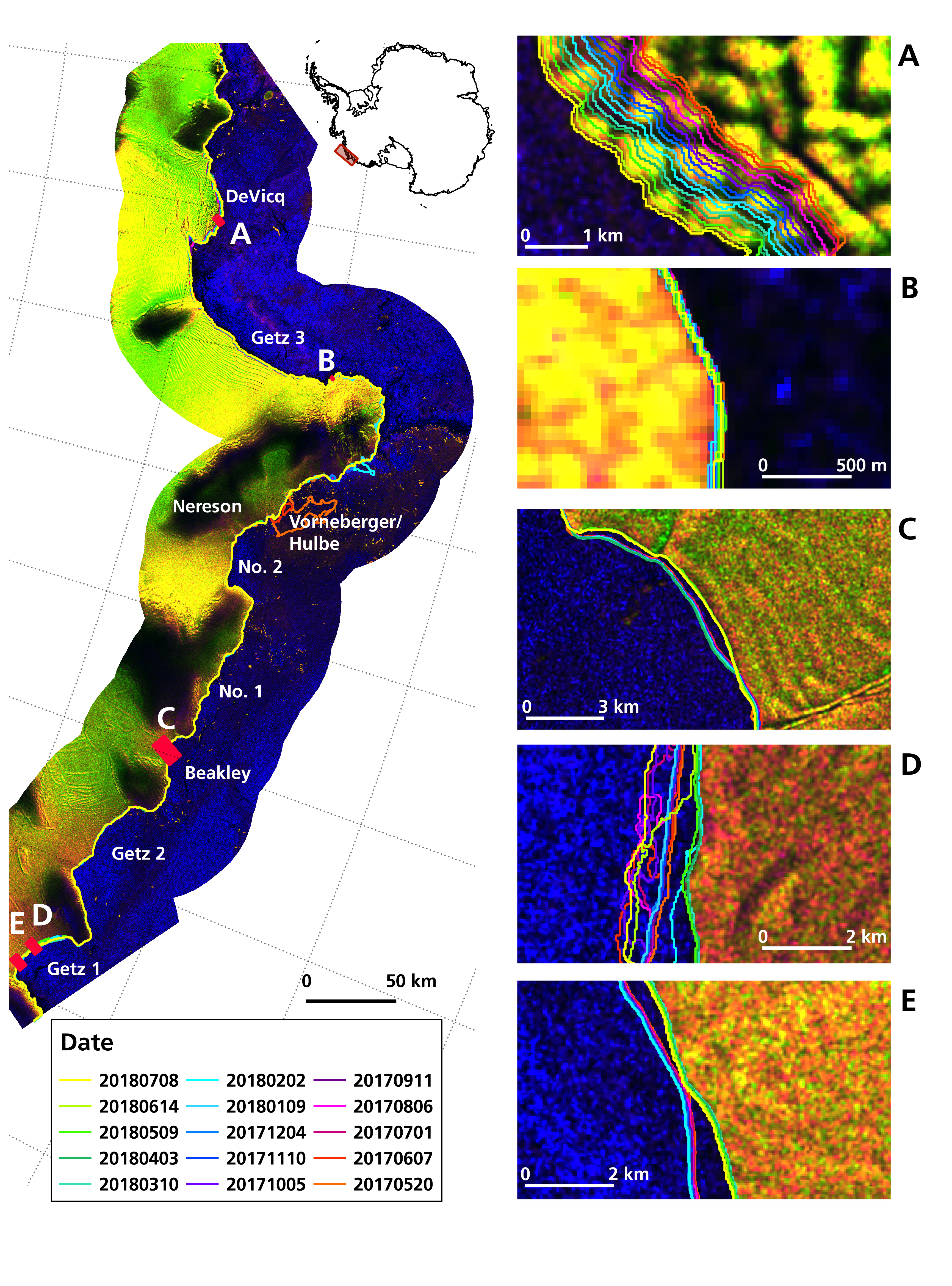
To develop a glacier and ice shelf front extraction algorithm, it needs to handle all kinds of different Antarctic coastline morphologies such as huge ice shelves, ridged glacier tongues, and solid rock. Therefore, we chose eight different training and test sites with different characteristics. The training areas are used to train the model and test it later on with new scenes over this region. Test areas are only used for testing the model and are not presented to the network before. All locations of the training and test sites are shown in Figure 1 and described in the following.

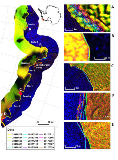
The area around the Sulzberger Ice Shelf is characterized by the fast moving Land Glacier (about 1.6 km/yr) and the slower moving glaciers (10-200 m/yr) flowing into the Nickerson (60 km wide) and Sulzberger Ice Shelf (more than 100 km wide) [29,30]. A huge ice shelf with a length of 400 km is represented by the Shackleton Ice Shelf site [31] with changing sea ice conditions. The part of Wilkes Land consists mostly of dynamic glaciers with myriads of icebergs and ridged glacier tongues. Additionally, sea ice conditions and mélange are challenging in this area. Finally, along Victoria Land, long glacier tongues enter the ocean between steep terrain. Later on, the developed workflow shall be tested on the following four test sites to demonstrate the transferability of our approach. Ekstromisen is a 143 km wide ice shelf along Queen Maud Land, far away from any training sites. The disintegrated Wordie Ice Shelf and the surrounding glaciers lay along the Antarctic Peninsula within steep terrain. The third test site is at Oats Land with long glacier tongues and ice shelves in different shapes. Lastly, a part of Marie Byrd Land is selected because of the multi-year ice areas. Within this area, the Getz Ice Shelf was also chosen to test our algorithm on time series generation as little is known about the current frontal fluctuations [2]. The Getz Ice Shelf is the largest ice shelf along West Antarctica with an area of 33,395 km² and pinned with islands along the front [32]. Getz experienced the highest mass loss compared to all other ice shelves along West Antarctica with −67.6 ±12 Gt per year between 2003 and 2008 [33]. Basal melt accounts for about three quarter of the mass loss and calving for one quarter [33] but can vary as Getz is subject to changeable ocean forcing conditions [32]. Between 2008 and 2013/2015 the glacier flow of glaciers feeding the Getz Ice Shelf increased by 10 to 100 m/yr at the grounding line (6% increase of discharge) [34]. The grounding line itself of the Getz Ice Shelf retreated 100–200 m per year between 2010 and 2016 [35]. Taken together, those factors indicate that Getz Ice Shelf is exposed to changing environmental conditions.

3. Input Data

3.1. Sentinel-1 Data

The Sentinel-1 mission is a constellation of two satellites with radar imaging sensors operating at C-band (5.4 GHz/5.6 cm). The two satellites Sentinel-1A (launch 2014) and Sentinel-1B (launch 2016) complement each other allowing six days revisit times or even less (in polar regions). For the Antarctic coastline, a high-resolution IW (interferometric wide-swath) mode with single HH polarization and 10 m spatial resolution exists. The other available imaging mode is the extra wide-swath (EW) with dual polarization HH+HV and a spatial resolution of 40 m. The EW product was selected over the higher resolution IW product because of the better spatial coverage and the two available polarizations which are crucial for ice type classification [36,37,38,39,40]. Additionally, the active microwave sensor acquires data independent from polar night and cloud cover ensuring continuous acquisitions compared to optical imaging systems. To train our DCNN, we use 38 pre-processed Sentinel-1 scenes covering the four training sites, Sulzberger Ice Shelf (20 scenes), Shackleton Ice Shelf (6), Wilkes Land (6), and Victoria Land (6) during various seasons with different sea ice conditions (see Table S1). We chose all available 20 scenes for the Sulzberger ice sheet to have one data set with all possible sea ice and backscatter variations through the year. The other training areas required fewer scenes but added different shapes of glaciers. Here, only every two months a scene was selected in the course of a year. The month June 2018 was excluded from every site as it is used for testing afterwards.

3.2. Antarctic TanDEM-X

The Antarctic TanDEM-X was acquired between April 2013 and November 2014 and is available with 12 m and 90 m spatial resolution. Over ocean areas, the DEM (digital elevation model) was edited to exclude error values over sea ice and icebergs. For the editing, the ice sheet was clipped to the TanDEM-X coastline product retrieved by thresholding on elevation and amplitude as well as manual editing afterwards. The 90 m DEM product is used in this study as only a rough value for elevation is necessary. Additionally, it reduces computation time. Elevation information is necessary as radar imagery water and the higher ice sheet have very low backscatter values. To reduce classification errors in those regions, the elevation information helps the model to distinguish those two classes better. As the DEM is only a rough orientation value, it does not matter that the fronts in the TanDEM-X are from earlier years.

3.3. Training Labels

To train a machine learning classifier, ground truth labels are necessary. For Sentinel-1 imagery, only a few manually delineated fronts in the Antarctic Digital Database (ADD) exist. In-situ measured front positions do not exist. Therefore, we had to create our own labels, which is a challenging task on SAR imagery and requires expert knowledge. Even in already existing manually delineated coastline products, huge differences can be observed. Especially in areas of multi-year sea ice, mélange, and glacier termini with icebergs, the coastline products differ. This demonstrates how subjective manual coastline and ice front delineation is and asks for a general definition. In order to create accurate and consistent front labels, we define the calving front as the border between ocean and land ice including floating ice shelves and glacier tongues. As soon as an iceberg calves and is no longer connected to the ice shelf or glacier, it is considered as ocean. For additional help and a better impression on the Antarctic coastline, we used previous coastline products from the MODIS Mosaic of Antarctica, the RADARSAT Antarctic Mapping Project, and the USGS (United States Geological Survey) Coastal Change Project and optical imagery from Bing Maps, Google Earth, and Landsat. The TanDEM-X digital elevation model helped to distinguish multi-year sea ice from shelf ice as sea ice is lower in elevation. Even though, we labeled the fronts in all conscience they still represent our subjectively defined front position. For the exact position of the coastline, ground truth measurements would have been necessary. A more detailed explanation of the training label selection is given in Section 4.3.

4. Method

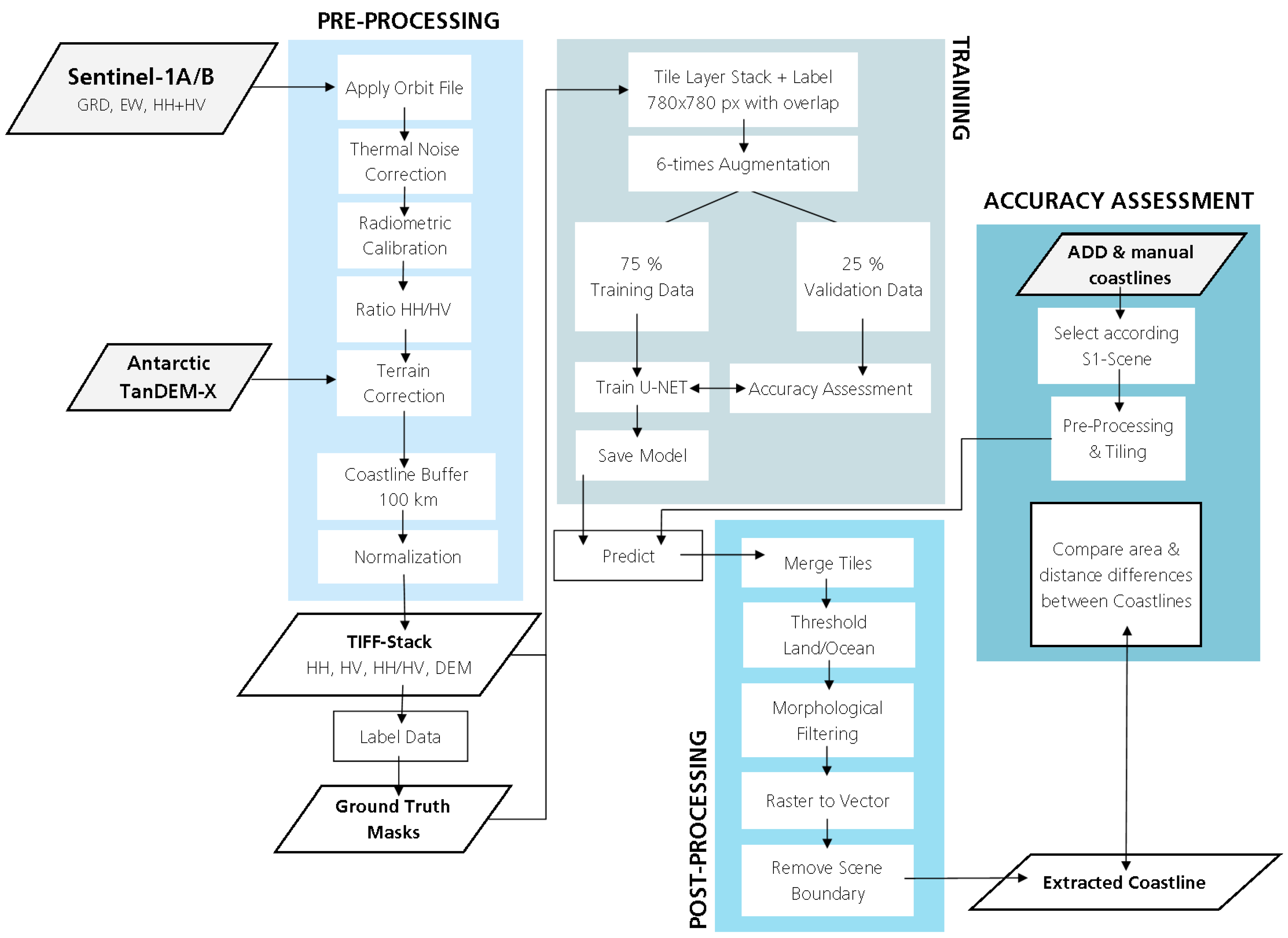
4.1. Pre-Processing SAR Data

The pre-processing of Sentintel-1 EW GRD (Ground Range Detected) scenes was performed with the ESA SNAP (Sentinel Application Platform) software 6.0 including the following steps:

• Apply Orbit File;
• Thermal noise removal;
• Radiometric calibration;
• Geometric terrain correction with TanDEM-X 90 m;
• Stacking of HH, HV, HH/HV, and TanDEM-X 90 m.

The Orbit File is applied to update satellite position and satellite velocity for more accurate orbit state vectors. Afterwards, thermal noise is reduced by the thermal noise removal. Radiometric calibration converts the backscatter intensity to the backscatter coefficient sigma nought. Now, the pixel values represent the backscatter of the reflecting surface and make comparison between different scenes possible. Usually, speckle filtering is applied afterwards but we decided to forgo this step as it might reduce the appearance of edges. Finally, to remove distance distortions in the signal due to topography, we corrected for terrain with the TanDEM-X 90 m. With the terrain corrected scene, a four-layer stack is created with the polarizations HH and HV, as well as the ratio HH/HV and the digital elevation model.

4.2. U-Net Architecture for Image Segmentation

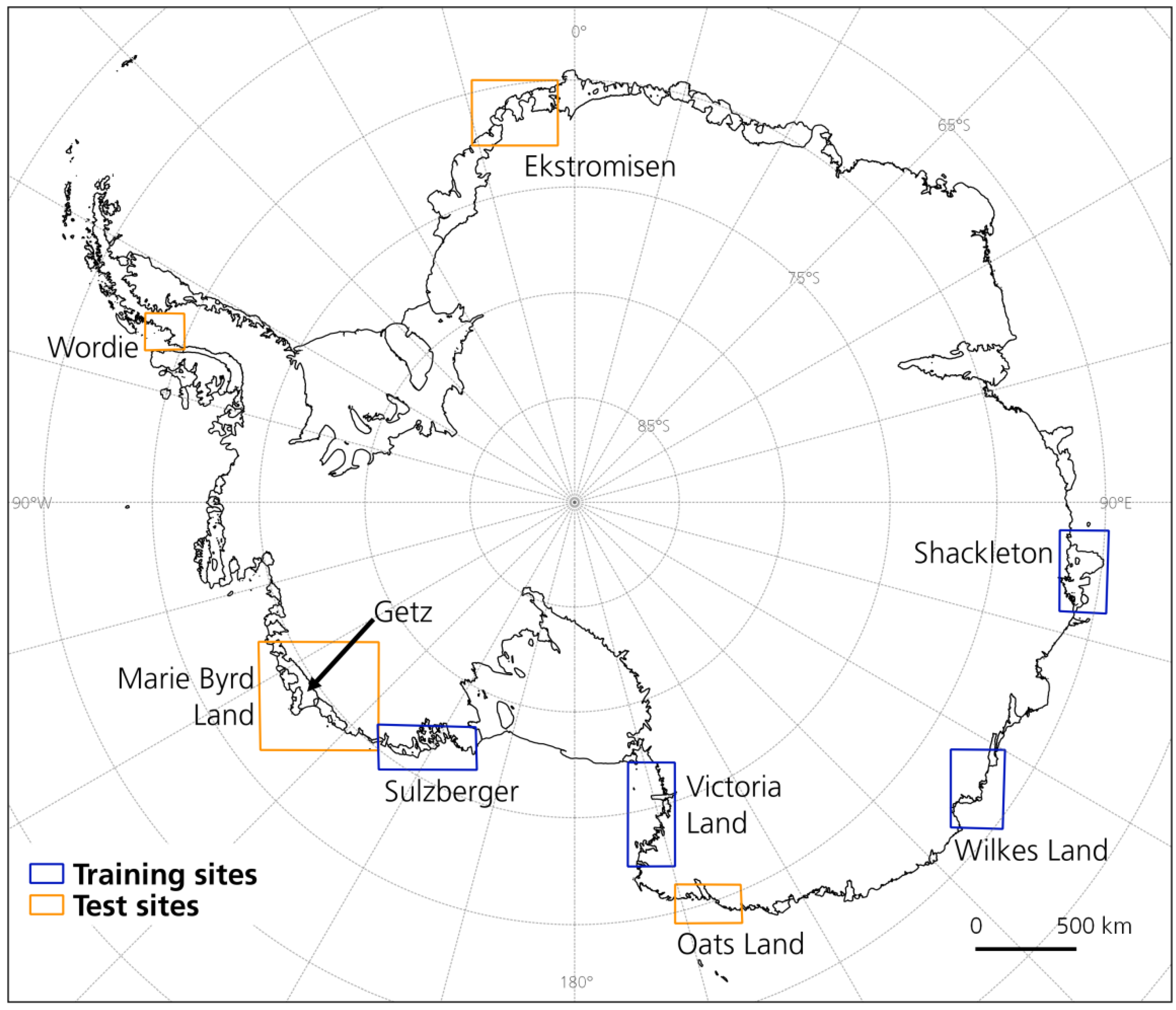
To extract the border between the two classes, land ice and ocean, we use a classifier which takes the pixel value as well as the spatial context into account. We chose the basic structure from the originally developed U-Net from Ronneberger et al. [22] and modified the architecture for our purpose. Main modifications include (1) the usage of bigger input tiles; (2) starting with 32 feature channels (instead of 64) and increasing only to 512 (instead of 1024); (3) including drop out; and (4) feeding four input channels instead of one. Figure 2 visualizes our modified U-net architecture with four down-sampling units (red arrows) in the encoder block and four up-sampling units (green arrows) in the decoder block as well as skip-connections (black arrows). In the following, we explain the basic function of the U-Net, hyperparameter selection, and why we entered modifications.

To train the network, we feed 780 x 780 pixel tiles with four input channels (HH, HV, DEM, HH/HV). Four input channels were selected to be able to not only use gray scale images but to include different polarizations and elevation information. The tile size was increased compared to the initial U-Net as bigger tiles include more spatial context, which is crucial for feature detection along the Antarctic coastline. For training, each of the input tiles is convoluted by a 3 x 3 kernel with stride 1. The kernel consists of a 3 x 3 matrix of random initialized weights which gets updated during the training process using the Adam optimizer in TensorFlow 1.12 with the default learning rate of 0.001, the default cost function categorical cross entropy and the activation function ReLU (rectified linear units). Also, bigger kernels were tested but increased the computational cost and were neglected. The trained weights can be seen as a filter that extracts specific features of the input image. Hence, after each convolution, feature maps are generated from the input image for the number of available filters. In our case, the four input channels are convoluted to 32, 64, 265, and 512 feature maps. As our input tiles and the glacial features are bigger than the cells in the medical imagery from the initial U-Net, we selected less but bigger feature maps. This keeps the computational cost low, whereas still enough trainable parameters are obtained. With each down-sampling block, the number of feature maps increases whereas the tile size decreases by a 2 × 2 max pooling operation. This technique allows reducing the image size and computational cost by taking the maximum value of each 2 × 2 pixel matrix. This extracts the most important information. After each pooling, dropout is applied to randomly exclude a given amount of the trained weights (for each training step) to prevent overfitting. Finally, at the end of the encoding block, 512 feature maps of the size 48 × 48 pixel exist.

Thereafter, the decoder block up-samples this densified information again to assign each pixel of the input image a classification result. Rows and columns of the input feature maps are repeated to increase the tile size to the initial input size. This step is connected to the previous feature map via convolution. The contextual information is derived from the encoder via the copy and crop skip connections. The last 32 feature channels are pooled by a 1 × 1 convolution with the Sigmoid activation function to obtain prediction probabilities for each class. Finally, the output image has the same size as the input image with two channels for the classification probabilities for each class (land ice/ocean). Our fully convolutional network consists of 7.8 million trainable parameters.

4.3. Training

For training, the final 38 scene stacks are normalized and then tiled into 780 × 780 pixel patches. The patch size is limited by GPU RAM and batch size. We chose the biggest possible tile size for a higher spatial context, accepting the drawback of small batch sizes as described by [22]. Tiling is done with a 200 pixel overlap to reduce image borders and increase training data. To increase training effectively, we sorted our scene tiles into tiles with border areas, tiles covering only one class, and tiles with coastline. The most important tiles covering the coastline were augmented six-times by flipping and rotating for 90, 180, and 270 degrees. This creates a more intense training on the calving front. For training, we only used 30% of the border tiles, 90% of the single class tiles, and all augmented calving front tiles. Finally, we had 19,576 patches, out of them we randomly selected 25% for validation. Validation data is important as it tells after how many epochs the model converges and training has to be stopped. We trained the U-Net with a batch size of two on a GeForce GTX 1080 GPU with 12 GB RAM. The model converged after 30 epochs with a dropout value of 0.3 (30% of the weights are randomly dropped after updating). This was empirically calculated and outperformed dropout with the values 0.0, 0.2, and 0.5. Also, batch normalization was tested but resulted in worse results probably because the batch size is very small. 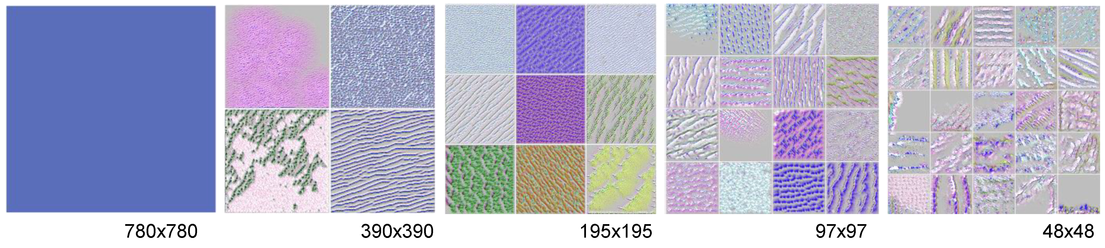Figure 3 is a visualization of some of the learned filters in the down-sampling blocks. From left to right, the image size decreases from 780 to 48 pixels. Low level features are recognized after the first convolution. For example, the first filter is sensitive to the HH polarization and the DEM information (R: HH, G: HV, B: DEM, alpha: ratio). After one pooling operation, the filters start to be sensitive to broader ice-related features. After more convolutions and pooling operations, the filters get much more detailed. Ice structures in various orientations can be recognized very clearly, especially for the last two down-sampling blocks. The trained weights are able to produce classification accuracies of 98.14% for the training and 98.16% for the validation data set (after 30 Epochs).

4.4. Post-Processing

The main reason for post-processing is to generate shapefiles from the classification results. First, we merge all tiles of each Sentinel-1 scene to a georeferenced raster tiff. In overlapping areas, the mean of both classification results is taken. The prediction probabilities from the U-Net are thresholded by 0.5, so every pixel classified with a 50% probability or higher is classified as land ice. Afterwards, morphological filtering is applied with the python package scikit-image. Holes in the ice area are closed before removing islands in the water (e.g., icebergs wrongly classified as land ice). The class land ice in the output raster is finally converted to a shapefile representing the extracted coastline from the initial Sentinel-1 scene. The above described framework is summarized in the flowchart of Figure 4.

4.5. Time Series Generation

A set of extracted calving fronts over the same area can be used to analyze calving front fluctuations. We extracted a 15-month time series from Sentinel-1A/B scenes in ascending mode. The distance change was calculated relative to an offshore baseline with the Digital Shoreline Analysis System (DSAS). Along the baseline, transects with 1 km spacing were used to measure the distance to the baseline at the intersection with the front position.

5. Accuracy Assessment

The performance of our framework is tested in two ways. First, we assess the classification accuracy for the two classes, land ice and ocean, after post-processing to compare our results with other deep learning studies. Second, the error is estimated by calculating the distance between the manually labeled coastline and the automatically extracted one. This is a better indicator for the distance deviation of the automatically extracted coastline to a manual one.

For testing, we use four satellite scenes covering the training areas in June 2018 as this month had not been used for training the network. Furthermore, four satellite images (also June 2018) covering the test sites are used for testing as well. Please see Table S1 for a list of all training and test scenes. As reference we use manually labeled coastlines for all training and test sites for June 2018. We selected this month as it was not used for training the model and because an external coastline from the ADD (Antarctic Digital Database) exists along Marie Byrd Land for June 2018.

The classification accuracy is calculated for a 1 km buffer area along the manual delineated coastline. We decided to focus on the frontal area only as classification accuracies for the entire 100 km buffer area are for all training and test sites over 99% and hence, less meaningful. Common standard performance measures (recall, precision, f1-score) are derived for the classification result. Especially to monitor calving front change, it is useful to also know the distance error of an automatically extracted coastline compared to a manual one. Therefore, we created for each training and test site a baseline for 1 km spaced vertical transects. These transects are automatically generated, only in areas of crossing transects or non-perpendicular transects we corrected them manually. Along those, the distance between both lines is calculated in Antarctic Polar Stereographic Projection. Transect generation and distance calculations were performed with the Digital Shoreline Analysis System (DSAS) provided by USGS. It is a free MATLAB-based tool which can run with ArcGIS.

5.1. Classification Accuracy

The classification accuracy is tested with the three standard parameters precision, recall, and f1-score for a 1 km buffer along the manual coastline for the classes land ice and ocean. Precision is a good measure for false positives, recall for capturing real positives and f1-score is the balance between both. The accuracies are given for June 2018 (

Table 1. Classification performance for all training and test sites (June 2018). High/low values are indicated in bold.

		Training Sites				Test Sites
	Accuracy measure	Sulzberger	Victoria Land	Wilkes Land	Shackleton	Marie Byrd Land	Oats Land	Ekstromisen	Wordie	Mean Train	Mean Test
ice	precision	0.85	0.89	0.87	0.92	0.91	0.92	0.91	0.85	0.88	0.90
	recall	0.85	0.98	0.92	0.96	0.94	0.91	0.94	0.91	0.93	0.93
	f1-score	0.85	0.93	0.89	0.94	0.93	0.91	0.93	0.88	0.90	0.91
water	precision	0.79	0.97	0.91	0.96	0.92	0.91	0.94	0.90	0.91	0.92
	recall	0.86	0.87	0.86	0.92	0.90	0.92	0.90	0.84	0.88	0.89
	f1-score	0.83	0.92	0.88	0.94	0.91	0.91	0.92	0.87	0.89	0.90

). The average f1-score for ice in all train sites is 90% and for the test sites 91%, for water 89% and 90%, respectively. Within the different training and test areas, the accuracy varies slightly. The classification for Shackleton Ice Shelf performed best with 94% accuracy for both classes. In contrast, Sulzberger Ice Shelf only reaches 85% for ice and 83% for water. Better performance can be reached for the test site Ekstromisen with 93% (ice) and 92% (water). The area along the disintegrated Wordie Ice Shelf has slightly lower accuracies with 88% for ice and 87% for water. In general, for ice classification the true positives are captured well but the lower value in precision indicates more false positives. Hence, a slight over-classification for the class land ice exists.

5.2. Error Estimation

The error of the automated coastline is presented as the distance difference to a manual delineated coastline. The difference can either be calculated along transects or as the average width of the enclosed area between the manual and automated coastline. The advantage of using transects is twofold. Transects can be drawn for selected sections along the coastline which allows to calculate the distance error for frontal sections and stable coastline areas separately. Additionally, with calculating the median instead of the mean distance of several transects, outliers can be eliminated and the estimated frontal change is more accurate.

A second way to calculate the error in distance is to divide the area difference of both coastlines (manual and automated) by their averaged length (short A/F). This way, the calculated error in distance can be calculated quickly but extreme values are smoothed out. Nevertheless, we calculated this often-used formula for comparison with already published studies.

The error estimation results are presented in

Table 2. Distance measured errors (in meters) along transects for frontal and stable coastline sections as well as the entire study region. An estimate for the difference between two manually delineated coastlines is given with the ADD (Antarctic Digital Database) coastline (mean error). A/F is the averaged width of the enclosed area between the automated and manual delineated coastline for each study region.

		Training Sites				Test Sites
	Measured Coastline	Sulzberger	Victoria Land	Wilkes Land	Shackleton	Marie Byrd Land	Oats Land	Ekstromisen	Wordie	Mean Train	Mean Test
mean	complete	267	112	153	72	118	162	126	210	151	154
	front	421	174	208	80	171	119	172	338	221	200
	stable	46	68	127	49	53	70	62	235	73	105
median	complete	8	-31	-13	-27	-7	4	-8	3	-16	-2
	front	20	-56	19	-32	-9	1	6	2	-12	0
	stable	-2	-25	-61	-22	-4	5	-12	15	-28	1
ADD	complete	1539	-	-	-	416	-	-	-	-	-
	front	3098	-	-	-	313	-	-	-	-	-
	stable	180	-	-	-	186	-	-	-	-	-
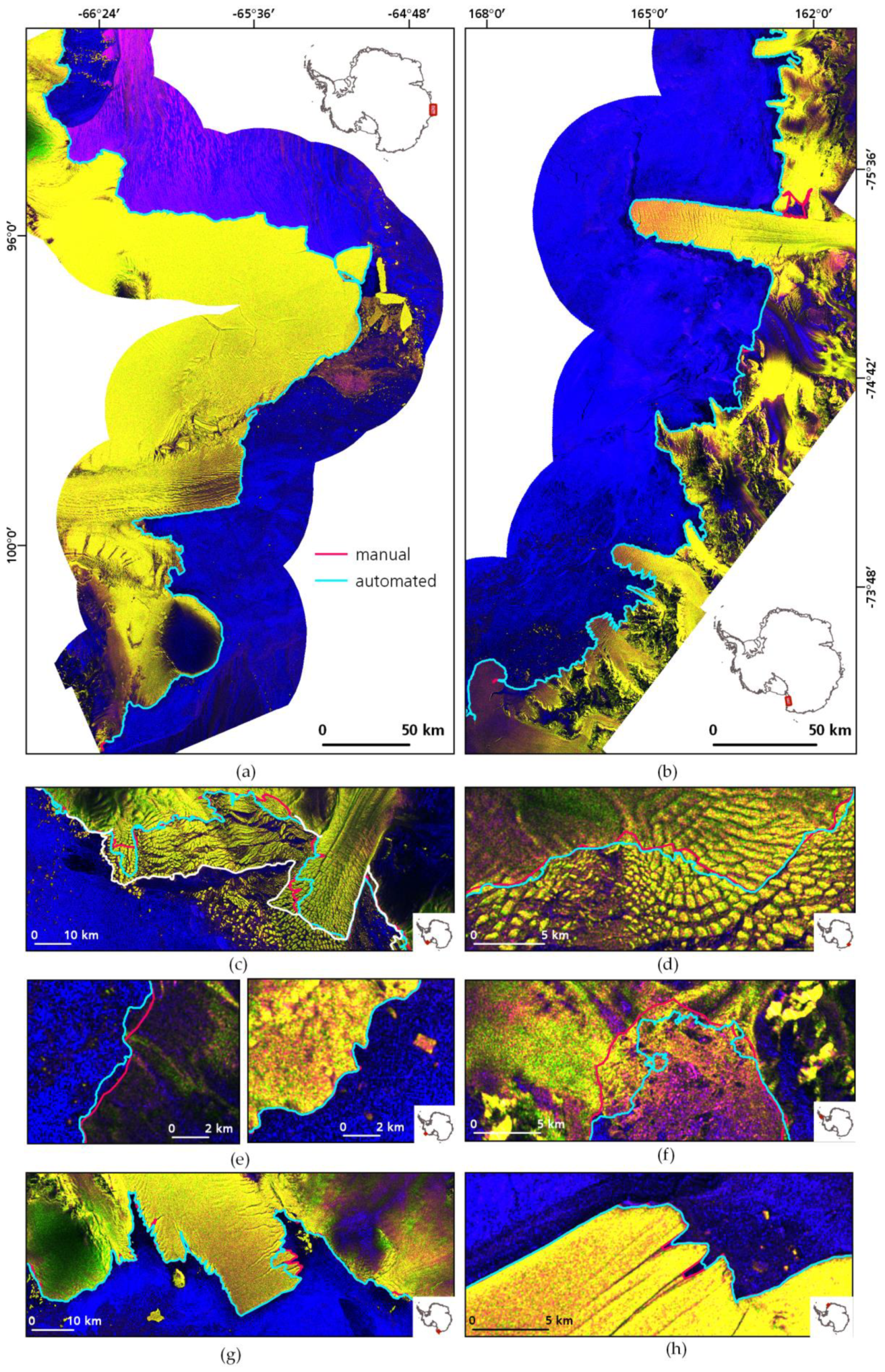
A/F	complete	121	103	35	54	108	104	66	153	78	108

with the absolute mean, the median, and the A/F value. The difference between the automatically extracted coastline and the manual delineation is on average 151 m for areas included in training and 154 m for test areas. For stable coastline areas, the error is lower as for frontal areas. Taking the median instead of the mean of all transect measurements, the error reduces to -16 m for training and -2 m for test areas. Best results are performed for the Shackleton and Ekstromisen Ice Shelf. Larger errors occur in the area of the Sulzberger Ice Shelf and the disintegrated Wordie Ice Shelf. To compare the achieved differences to the error between two manually delineated coastlines, we chose the ADD coastline for Marie Byrd Land which was delineated manually on the same Sentinel-1 scenes. Unfortunately, the error is quite huge as the ADD coastline was not very accurately delineated, including many areas of fast ice and calved glacier ice (see Figure 5 and Figure S1). Hence, the error for frontal areas only and the entire coastline is overestimated. The error in stable areas could still be a good indicator of a manual delineation error as the subjectivity in glacier and ice shelf front definition is excluded. The average error between two manual delineations is 180 m and 186 m for the Sulzberger Ice Shelf and the remaining Marie Byrd Land, respectively.

In general, the average width of the enclosed area is lower than the error calculated with transect-measurements. For training areas, the error is less than 2 px (78 m) for training, and 2.69 px (108 m) for test areas.

5.3. Time Series Evaluation

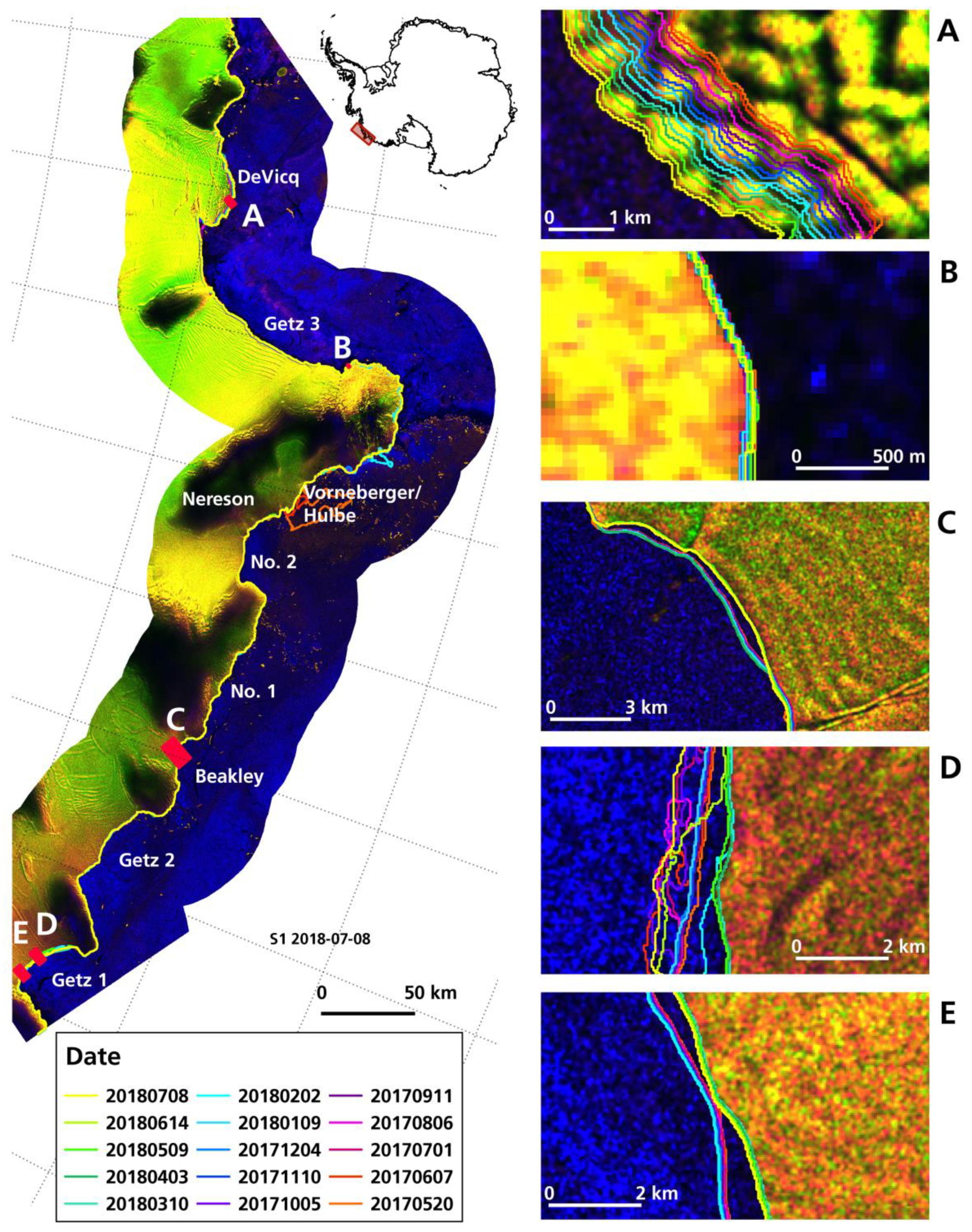
To assess how good calving front change can be tracked with our approach, we compare the presented 15-month time series with five manual delineated coastlines (see

Table 3. Error calculation for the Getz time series with five manual reference coastlines. The distance to the reference coastlines is presented as the absolute mean of the measured transect values.

	Distance (Absolute Mean) to Manual Reference (m)					abs. metrics (m)
	05-2017	07-2017	12-2017	03-2018	07-2018	mean	sd
Beakley	34	41	71	98	56	60	26
DeVicq	43	185	91	87	91	99	52
Getz 1	72	237	433	1018	1103	573	464
Getz 2	36	23	101	79	79	64	33
Getz 3	48	31	76	44	53	50	16
Nereson	149	43	72	134	60	92	47
No. 1	44	29	63	61	82	56	20
No. 2	40	29	45	77	58	50	18
Vorneberger/Hulbe	-	156	193	164	132	161	75

for dates) covering different months. The error is presented in Table 3 and

Table 4. Error calculation for the Getz time series with five manual reference coastlines. The distance to the reference coastlines is presented as the median of the measured transect values.

	Distance (Median) to Manual Reference (m)					abs. metrics (m)
	05-2017	07-2017	12-2017	03-2018	07-2018	mean	sd
Beakley	−17	−30	−66	−91	−49	51	29
DeVicq	5	42	−24	−50	−52	35	20
Getz 1	−37	−50	−146	−75	−1231	308	518
Getz 2	−29	−9	−84	−78	−73	55	33
Getz 3	−20	8	−64	−36	−38	33	21
Nereson	−32	5	−43	−107	−49	47	37
No. 1	−23	−19	−71	−58	−71	48	26
No. 2	−12	9	−48	−71	−47	37	26
Vorneberger/Hulbe	-	−5	−97	−73	−65	60	39

as the absolute mean and the median of the differences between the five reference coastlines and the automatic extracted one. The median is a more robust measure as it compensates errors and extreme values. The comparison of absolute mean and median calculations in Table 2 and Table 3 demonstrate that the difference between the automated and manual coastlines is smaller when using the median. We also present the absolute mean error with standard deviation for each glacier/ice shelf. Overall, the distance error is 1-2 px with some exceptions for the Vorneberger/Hulbe Glacier and Getz 1 (see Table 3 and Table 4).

To assure the reliability of our generated time series, we added a quality threshold. In some months with difficult sea ice conditions, extreme over estimations of land ice can occur. To exclude those miss-classifications, we added an outlier detection that removes extreme front positions with a distance greater than the one and a half times of the upper interquartile range plus the 90%-quantile. Additionally, we calculate the R² of the calculated regression through the time series for each glacier. In case the frontal change shows a clear signal in advance or retreat, the R² value will be high. Low values can indicate that a front experienced a major calving event or periodic calving.

6. Results

6.1. Mapping Results

Samples of the extracted coastlines are presented in Figure 5. The most accurately extracted coastline for the Shackleton Ice Shelf is presented in Figure 5a with a mean A/F deviation of 54 m. The turquoise coastline was automatically extracted and the manual reference is shown in magenta. The icebergs in front of the shelf are excluded from the ice shelf and only the huge, almost broken off, iceberg is correctly considered as ice shelf. In contrast, the coastline of Victoria Land (Figure 5c) deviated on average for 103 m. Specifically, the enclosed but open water area besides the Drygalski Glacier Tongue was not delineated accurately as it was closed in the post-processing step. Also, in parts of dark glacier surface and steeper terrain, slight deviations exist. For all other study regions, we selected snapshots of areas with delineation errors to assess weaknesses of our approach (Figure 5c–h). Figure 5c shows the Land Glacier of the training region “Sulzberger Ice Shelf”. As a manual delineated coastline from the ADD exists for the same date, it is shown in white for reference. This is a very good example of how subjective front delineation can be, as the two manual fronts deviate several kilometers in the area where calved glacier ice is trapped at the glacier fronts. The example for Wilkes Land (Figure 5d) shows only slight differences in the manual and automated results. Here it is often difficult to judge whether an iceberg already calved. Hence, the deviation is mostly only the width of an iceberg. Challenges due to radar shadow are demonstrated in Figure 5e. The front of the Siple Dome is clearly visible at the sensor facing side (Figure 5e, right). In the sensor turned away slope of the Siple Dome, the front is difficult to detect as the radar shadow darkens this area and lowers the contrast. For the area around the disintegrated Wordie Ice Shelf, robust results were obtained along stable coastline areas (Figure 5e, left). Major deviations just occurred in front of the right branch of the Flemming Glacier and Prospect Glacier with a lot of mélange and icebergs at the front (Figure 5f). The region Oats Land was extracted almost perfectly. Only a part of the Rennick Ice Shelf was not recognized as properly as it should be (Figure 5f). Very accurate results were obtained for the Ekstromisen Ice Shelf with only little deviations in the lateral crevasses of the ice shelf fronts.

6.2. Time Series Getz Ice Shelf

The time series of glacier and ice shelf front fluctuations was created for the Getz Ice Shelf from May 2017 to July 2018, limited through scene availability (see Table S2 for used scenes). The coastline extraction algorithm performed well in this test region. The advance of the DeVicq Glacier is very accurately extracted as can be seen in Figure 6A. In comparison, in stable areas the coastline is detected at almost the same spot (Figure 6B). Figure 6C demonstrates at the Beakley Glacier how good calving events of small widths (315 m) are captured. Calving events were also detected at the Getz 1 Ice Shelf (Figure 6E). Besides these accurate results, two errors occurred. A piece of the Getz 1 front is randomly miss-extracted (see Figure 6D). Additionally, in May and June 2017 a huge mélange area was misclassified in front of the Vorneberger and Hulbe Glacier (see Figure 6).

With the DSAS tool, a time series of glacier front fluctuations for all major calving fronts was generated. Figure 7 shows the relative advance/retreat compared to May 2017. Obviously, the DeVicq Glacier has the highest advance rate with 726 ± 20 m/yr, and Nereson Glacier with 23 ± 37 m/yr the lowest (see

Table 5. Glacier change rates per year with mean standard deviation from Table 4 and R-square of the linear regression.

Glacier/Ice Shelf	m/yr	R2
Beakley	−170 ±29	0.24
DeVicq	726 ± 20	0.95
Getz 1	37 ± 518	0.00
Getz 2	222 ± 33	0.82
Getz 3	463 ± 21	0.99
Nereson	23 ± 37	0.23
No. 1	52 ± 26	0.77
No. 2	141 ± 32	0.98
Vorneberger/Hulbe	232 ± 39	0.98

). The time series of Getz 1 and Beakely are the only noticeable fronts not following the general, almost linear advance. Beakely Glacier retreated by −170 m/yr. For Getz 1, the earlier mentioned miss-classifications (Figure 6D), which were not detected by our outlier detection, distract the time series. On the contrary, the miss-classifications in front of the Vorneberger/Hulbe Glacier are well detected with our outlier detection and excluded from the linear regression calculation to estimate average calving front movement. On average, the absolute mean of the distance error compared to a manual delineated coastline is relatively low with 75 ± 181 m for the entire front of the Getz Ice Shelf.

7. Discussion

7.1. Coastline Extraction

Glacier and ice shelf front dynamics are closely connected to the mass balance of the Antarctic ice sheet, explaining why a continuous, automated extraction of these fronts is desirable. Unfortunately, calving front monitoring from remote sensing imagery has been a challenging task due to changing sea ice conditions and mélange at the calving front. This lowers the contrast between land ice and ocean, making the glacier and ice shelf front extraction very challenging. Within the last years, CNNs performed well for coastline extraction on non-polar environments, which yields potential for the application on polar coastlines if the low contrast between different ice types can be tackled [19,26]. Recent studies on single glaciers presented first achievements by implementing convolutional neural networks for glacier front detection [27,28]. Those studies concentrated on single glaciers and their frontal dynamics by training a neural network on that specific region with a very high amount of training scenes. Here, a novel workflow for glacier and ice shelf front extraction has been proposed by taking advantage of the current developments in deep learning for computer vision combined with radar remote sensing data. Compared to previous studies, we improved the calving front extraction through the implementation of a U-Net, allowing for spatial and temporal transferability. The key innovations are the usage of multi-channel input data for more accurate classification results, the applicability for the Antarctic coastline with complex ice conditions, as well as the transferable applicability for large-scale coastal change analysis on a monthly scale. The created time series of monthly calving front fluctuations allow for the detection and dating of calving events for large-scale areas. This reveals changes in glacier and ice shelf extent on a so far unpreceded spatial and temporal scale and can give insights into current Antarctic coastal change dynamics.

Within our training and test sites, differences in obtained accuracies occurred. Interestingly, overall classification accuracies were almost similar for the training sites compared to the test sites. On average, the coastline deviated 151 m for training and 154 m for test areas measured along transects. Calculating the deviation with the A/F method, the training areas deviated less with 78 m compared to the test areas (108 m). One would have expected better results for areas included in the training as the network recognizes the specific shapes. But for training areas, as well as for test areas, better (Shackleton, Ekstromisen) and worse results (Sulzberger, Wordie) exist. It seems that the accuracy is rather dependent on the complexity of the region. For example, the area around the Sulzberger Ice Shelf has many fast ice areas that are challenging to detect (see Figure S2), which can also be seen by the results of Liu and Jezek [8]. They had to edit their automated coastline for those multi-year sea ice areas. Also, Wilkes Land has challenging fronts as it is often difficult to judge whether an iceberg has calved in this area (see Figure 5d). The area around the former Wordie Ice Shelf illustrates that in areas with low contrast, steep terrain, and mélange, the classification is less accurate. For better results, training areas along the Antarctic Peninsula should be included as terrain and glacier size are different from the existing training set. Results with higher accuracies were obtained for Ekstromisen, Marie Byrd Land, and Oats Land. Those regions were not presented to the network before but are more accurately delineated as some of the training areas. Those fronts are easier to detect as less difficult mélange and iceberg features exist and the contrast between ocean and land ice is higher.

Additionally, the method for accuracy assessment should be considered, as the results differ depending on accuracy measure (see Table 2). Many different ways exist to assess glacier change, with their advantages and drawbacks [41]. Our calculations via enclosed area and transects illustrate the differences. Wilkes Land is a good example to demonstrate differences in accuracy measure. The deviation of 153 m measured along transects is 4-times higher compared to 35 m calculated with the A/F method. The very long coastline through many small glaciers and bays compensated for the higher difference along transects. Comparing the average results for training and test areas, the values are quite close no matter what measuring technique was chosen and only deviate 5–6 m. By calculating the median of the transect measurements, the distance error is less with -31 to 8 meters. But it should be mentioned that calculating the median for the entire test or training site is less applicable if only selected glaciers are expected to be analyzed. In this case, the median has to be calculated for each front separately, which leads to an error of 1–2 px (see Table 4), but is still more accurate than the absolute mean.

Compared to existing studies, we were able to increase the classification accuracy from 92.4% for the training and 93.6% [27] for the validation data set to 98.1% and 98.2%, respectively. The training scene inputs from recent studies were also reduced from 123 images [27] and 75 images [28] to 38 images. Additionally, using several input layers with different polarizations and also the selection of bigger training areas, including a wide selection of coastline shapes, helped to reduce the training input. Additionally, wise selection of training tiles and only augmentation on prioritized tiles reduced the required training epochs. The deviation in distance to a manual front is comparable to previous published studies [27,28]. We achieved on average 1.96 px (78 m) for training and 2.69 px (108 m) for test areas. This is comparable to the work from Mohajerani et al. [27]. A slightly higher error was published by Zhang et al. [28] with 104 m (17.3 px). Here, the much higher spatial resolution of 6 m does not seem to improve the distance error in this case. Even though more detailed ice structures can be extracted from higher resolution imagery, the spatial context is lower in each image tile, which decreases the performance of the U-Net. In comparison, Krieger et al. [17] achieved slightly worse results with their edge tracing algorithm with deviations of 159 m (TerraSAR-X) vs. 246 m (S1). Here, the higher resolution satellite imagery seems to improve the extraction result. Sohn and Jezek [15] achieved accuracies of 2–3 px (approx. 200 m). Depending on the region and glacier morphology, the error of manual delineated coastlines lies in the same range of automated results. Manual delineations deviate on average between 38 m [28], 92.5 m [27], and 183 m (as we calculated for entire Marie Byrd Land). Conclusively, our approach can automatically extract Antarctic coastlines and still keep up with manual delineation accuracies.

7.2. Time Series of Getz Ice Shelf

A 15-month time series of calving front fluctuations was extracted to demonstrate transferability in space and time. Accurate results were obtained with a minor deviation of 75 ± 181 m on average, compared to manually delineated coastlines. The high standard deviation can be explained as a part of Getz 1 was extracted erroneously. This was probably caused by radar shadow, as the part of the Getz 1 front behind Wright Island appears much darker than the rest of the area. Radar shadow also occurred at the Siple Dome. Here, the two erroneous fronts of Vorneberger and Hulbe Glaciers were successfully removed by our outlier detection. To improve our proposed method, radar shadow areas could be masked to avoid false classifications. In all other cases, the fronts were extracted precisely. Even slight advances of 1 px per month were tracked as shown at the DeVicq Glacier front (Figure 6A). In case of calving events, they were captured exactly as demonstrated for the Beakely Glacier. All in all, the workflow allows an efficient processing and accurate assessment of current Antarctic calving front dynamics, which has not been possible with manual delineation.

The extracted time series along the Getz Ice Shelf presents a steady advance in all analyzed calving fronts (except Beakley and the erroneous front of Getz 1). But it should be noted, that the observation period is short and the observed advance could be interrupted by calving events at any time. Nevertheless, only a few of the fronts show an advancing tendency indicated by high R-square values. The fronts of DeVicq, Getz 2 and 3, No. 2, and Vorneberger/Hulbe advance significantly whereas the advance of No. 1 and Nereson Glacier is close to zero and lower than the standard deviation of measurement. Hence, those glaciers were comparatively stable during the period of measurement. Analyzing the time series for the Beakley Glacier, the sudden drop in advance indicates a calving event between April and May 2017.

The current calving front fluctuations show in some cases contrasting tendencies compared to previous observations. The Getz Ice Shelf was described as a pretty stable ice shelf with phases of slight retreat and advance [29]. DeVicq Glacier is one of the fast flowing glaciers along Marie Byrd Land [42]. Between 1973 and 1988, the glacier retreated 5 km [43], and 18.6 km between 1973 and 1997 [29]. Compared to available coastline products (see Section 3.3 for products), the retreat from the maximum extent in 1973 decreased slightly in the 1980s and further until 1997. Since then, a phase of advance started until our last measurement in July 2018, when the maximum extent of 1973 was almost reached. With the current speed of 726 ± 40 m/yr the maximum extent from the 1970s would be reached in 2020. For the remaining Getz Ice Shelf, the fronts were almost stable between 1973 and 1988/1990. Only at Getz 2 the front retreated 2 km. Compared to the coastline of the USGS mapping project, the current front is around the stage of the 1980s and slightly lower in extent than the maximum extent in the 1970s. Getz 3 experienced retreat between the 1970s and 2014. Since then a phase of advance started, compared to the referred coastline products. Changes in retreat to advance of the ice shelf front can have many reasons. Jacobs et al. [32] emphasized the very changeable ocean forcing for the Getz Ice Shelf which might also influence front position. They are closely connected to changes in wind conditions and sea ice cover. Sea ice cover days between 1979–2000 were pretty much equal along the Getz Ice Shelf but reduced between 2000–2012 [44]. Further investigations are necessary to assess the possible connections between reduced buttressing due to less sea ice cover and advancing fronts of the Getz Ice Shelf.

8. Conclusions

This study presents a novel workflow to extract Antarctic glacier and ice shelf fronts based on a convolutional neural network. The core of our approach is a modified U-Net to segment dual-pol Sentinel-1 scenes into land ice and ocean and to extract the coastline in-between afterwards. Spatial and temporal transferability is demonstrated on eight training and test sites. The mean deviation between our automated results with manual delineated coastlines is on average 78 m and 108 m for training and test areas, respectively. Results are obtained for all training and test areas with best performances for huge ice shelves such as Shackleton and Ekstromisen and slightly lower accuracies for areas including fast ice, mélange, or steep terrain causing radar shadow (e.g., Sulzberger, Wordie). The applicability of our approach to automatically track calving front dynamics on a high temporal and spatial scale is demonstrated on the time series along the front of the Getz Ice Shelf. Even small calving events could be captured and dated. The majority of the front along the Getz Ice Shelf shows a general tendency of advance between May 2017 and July 2018. The fastest advance is measured for DeVicq Glacier with 726 ± 20 m/yr.

In the future, the spatial and temporal transferability of our approach will allow the assessment of the Circum-Antarctic calving front dynamics after adding more training sites. This could provide new insights into the current dynamics of Antarctic coastal change and help to link environmental forcing to glacier and ice shelf front extent fluctuations.