An Empirical Assessment of Angular Dependency for RedEdge-M in Sloped Terrain Viticulture


Environmental Remote Sensing and Geoinformatics, Trier University, 54286 Trier, Germany
*
Author to whom correspondence should be addressed.
Remote Sens. 2019, 11(21), 2561; https://0-doi-org.brum.beds.ac.uk/10.3390/rs11212561
Submission received: 2 September 2019
/
Revised: 25 October 2019
/
Accepted: 29 October 2019
/
Published: 31 October 2019
(This article belongs to the Special Issue Remote Sensing in Viticulture)
Abstract
:For grape canopy pixels captured by an unmanned aerial vehicle (UAV) tilt-mounted RedEdge-M multispectral sensor in a sloped vineyard, an in situ Walthall model can be established with purely image-based methods. This was derived from RedEdge-M directional reflectance and a vineyard 3D surface model generated from the same imagery. The model was used to correct the angular effects in the reflectance images to form normalized difference vegetation index (NDVI) orthomosaics of different view angles. The results showed that the effect could be corrected to a certain scope, but not completely. There are three drawbacks that might restrict a successful angular model construction and correction: (1) the observable micro shadow variation on the canopy enabled by the high resolution; (2) the complexity of vine canopies that causes an inconsistency between reflectance and canopy geometry, including effects such as micro shadows and near-infrared (NIR) additive effects; and (3) the resolution limit of a 3D model to represent the accurate real-world optical geometry. The conclusion is that grape canopies might be too inhomogeneous for the tested method to perform the angular correction in high quality.
1. Introduction
The concept of precision viticulture [1] has rapidly developed and extended to a variety of unmanned aerial vehicle (UAV) applications in recent years. These include digital 3D vineyard structure reconstruction from UAV imagery for precise row monitoring [2,3] and crop status quantification, such as evaluating growth conditions with hyperspectral sensors [4], RGB, multispectral, thermal sensors combined together [5], and utilizing machine-learning techniques for multispectral sensors to schedule the irrigation [6]. All of the mentioned quantification works have used optical sensors, which heavily rely upon the accurate derivation of canopy reflectance.
In viticulture, this demand faces two unique geometric problems. First, the canopy converges to a narrower shape after pruning, limiting the retrievable information from nadir orthophotos. Second, although the former problem can be improved by tilting the camera’s view angle to observe the side of the canopies, the enlarged sun-target-sensor angle in the sloped areas will further interfere with the target reflectance anisotropy. The resulting consequences have been demonstrated in other scenarios. One study on wheat [7] showed that SCOPE-modeled directional reflectance was largely different from the UAV hyperspectral spectrometer measurement in low-tilt angles. Another hyperspectral study [8] highlighted the influence of viewing geometry on the Normalized Differential Vegetation Index (NDVI) values, demanding the necessary compensation.
The angular reflectance dependency has been intensively studied within the framework of the bidirectional reflectance distribution function (BRDF) [9]. For vegetation canopies, the anisotropic reflectance can be dependent on the canopy structure (surface curvature, leaf layers, shadow proportion, leaf orientations, etc.) and visible background at different view geometries. This has resulted in a series of modeling tools. One of the commonly used models was described by Walthall et al. [10]. It was then improved in a detailed layout in Nilson and Kuusk’s work [11], which was illustrated by Beisl et al. [12]. Another commonly used model was proposed by Rahman et al. [13]. These models have been used to semi-empirically establish the relation between canopy directional reflectance and geometry. Further modeling with BRDF simulation tools, such as PROSAIL [14,15], can also be found in application reviews [16].
Early works have used ground goniometers to study the angular reflectance dependency [17,18]. But by paralleling the goniometer measured ground truth and UAV measurements, studies have already shown that the UAV-mounted cameras can obtain bidirectional reflectance factors without ground measurements. For example, a correspondence was found between goniometer and UAV commercial camera on a smooth snow surface [19]. A low standard deviation between goniometer and UAV directional reflectance on reference panels was found in another study [20]. By involving a sun sensor, UAV directional reflectance can also be derived without a reference panel [7,21,22]. Such a method was tested and evaluated in a very recent work, where high correlation coefficients were found between UAV measurement and literature goniometer values on a spectralon white reference panel [23].
A range of dedicated UAV reflectance anisotropy studies have been conducted on different types of vegetation. Aside from the wheat study mentioned before [7], another hyperspectral study on wheat and barley [24] found that the scattering parameter in the Rahman–Pinty–Verstraete model differed by the crop heading stage. It also found a strong backscattering reduction in potato after the full coverage of canopies [25], indicating the potential of crop-growth stage monitoring by angular observation. Taking the bidirectional effect into consideration, the radiometric correction via geometric block adjustment method [26,27] was developed to significantly improve the uniformity of spectral mosaics. Another assessment study of BRDF in UAV near-infrared (NIR) imagery has illustrated the compensation method for angular radiometric disturbances [28].
As part of a UAV-monitoring project on a sloped vineyard, this paper focuses on delivering a feasible approach to sample, model, and correct the angular dependency for the vine canopy reflectance from UAV imagery without field measurements. In the study, the UAV carried a tilted RedEdge-M sensor to take the images from a sloped vineyard. The reflectance anisotropy was studied on these images by combining the RedEdge Python package [29] and the 3D-reconstruction software Agisoft© Metashape [30] applications. Then, both the corrected and uncorrected reflectance images of the red and NIR bands were used to compute their side-view orthomosaics and corresponding NDVI maps from different directions.
The goal of this study is to deliver a 3D NDVI surface that is independent of the angular effects. The hypothesis is that the corrected NDVI values from different views should be significantly lower than the uncorrected ones.
2. Materials and Methods
2.1. Study Area, UAV Trials, and Materials
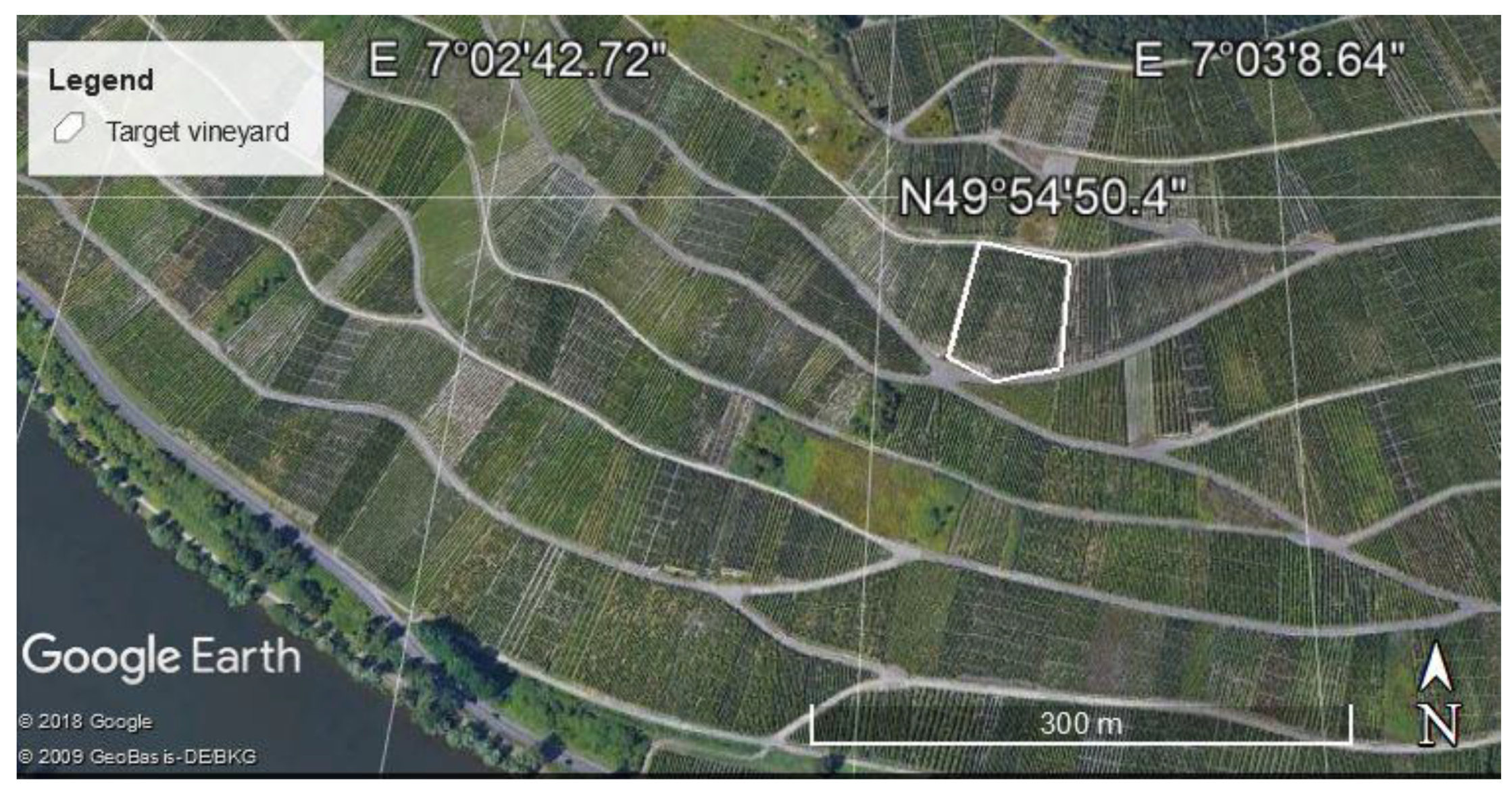
The study area is located at Bernkastel-Kues, Germany, a Riesling vineyard on the Mosel valley (Figure 1). The vineyard slope angle is around 19°, facing southwest. The average row distance is 1.3m, and the average canopy distance is 1.2m. The soils between rows were slightly weeded. For the BRDF study in this paper, the particular imagery on 13 July 2018 was used, just 2 weeks after pruning. The time point was between fruit set and veraison.
The UAV is an RC-Upgrade© BlackSnapper-L-pro quad helicopter frame cored with a DJI© A3 flight control system. The MicaSense© RedEdge-M is a 5-discrete-narrowband frame multispectral sensor that is commonly used in remote-sensing studies and precision agriculture. The band information is summarized in Table 1. It contains a downwelling light sensor (DLS) module that measures the ambient light for each spectral band during flight [31]. It is also configured with a 3DR© GPS (accuracy, 2–3 m) and a 3-axis magnetometer module that records the UAV’s exterior orientation for each capture. This information is used to geometrically trace back the illumination on each specific field of view (FOV) for direct reflectance computation.
The flight lasted around 12 minutes (from 11:39 to 11:51), during which the camera was configured 20 degrees zenith from nadir, always toward the northwest. There was no wind during the flight. The flight altitude was kept at around 242 m above sea level (30–50m relative to the slope). The nadir pixel resolution was around 2.6 cm.
The 3D processing was conducted in Agisoft© Metashape 1.5.1. After 3D processing, the report showed that GPS errors ranged from 0.8~3 m. Image-wise geometric analysis and correction were processed in Python, with certain original codes from RedEdge-M packages modified. Sampling points allocation, canopy mask building, NDVI computation, and results visualization were conducted in ESRI© ArcGIS [32].
2.2. BRDF Sampling, Modeling, and Correction
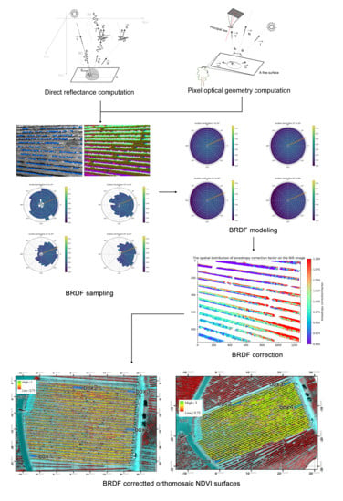
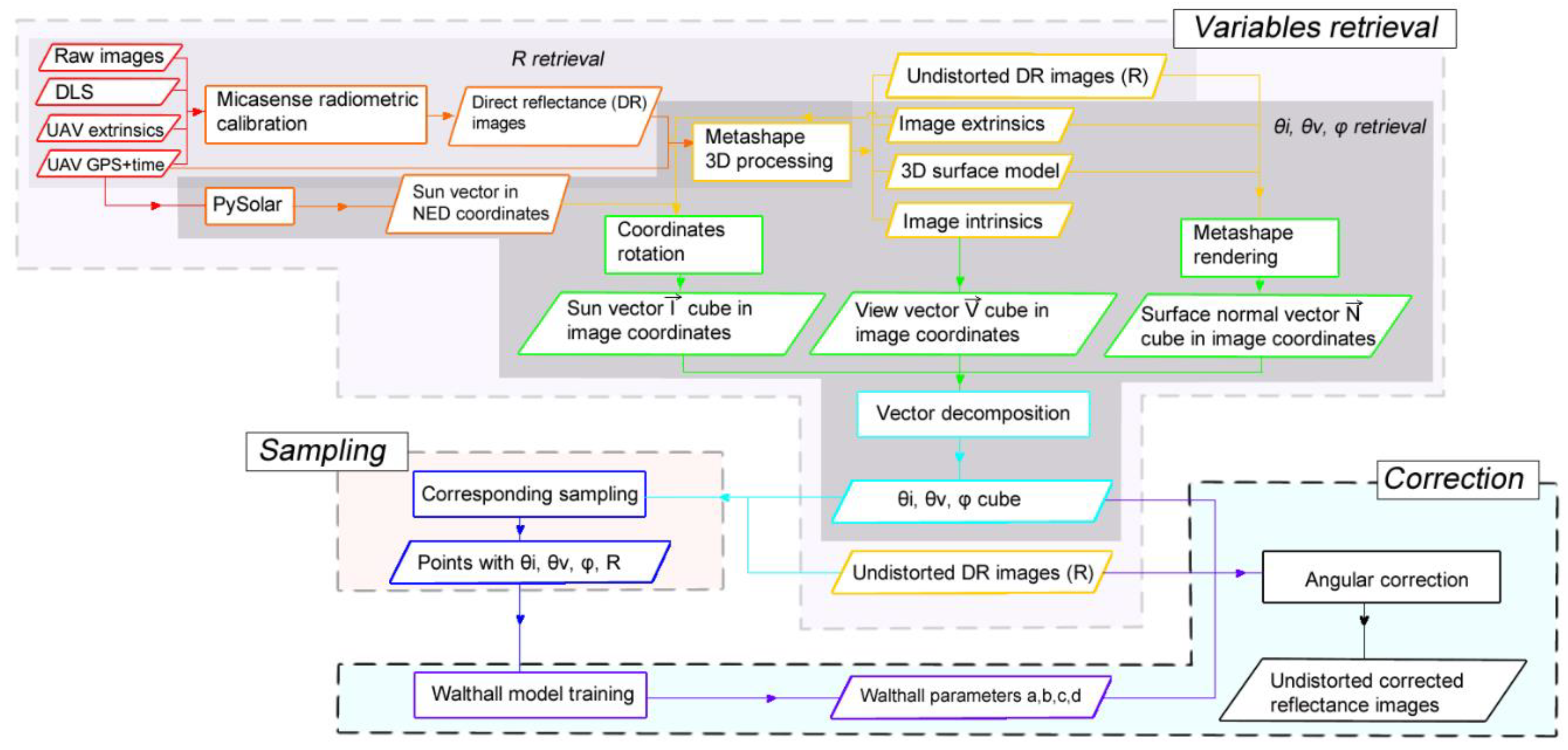
As illustrated in the schema (Figure 2), the whole procedure can be divided into three major modules: BRDF variables retrieval, sampling, and correction. The variables retrieval can be further divided into two sub-modules: the direct reflectance (R) retrieval and the geometry (θi, θv, and φ) retrieval.
This study utilized the Walthall model [10,11,12] in Equation (1), which was developed for homogenous spherical canopies such as wheat and soybeans. For computation, the variables consist of two major compartments: (1) the dependent variable reflectance factor R and (2) the independent geometric variables.
where:
- R—the observed directional reflectance factor;
- θi—the solar incident zenith;
- θv—the view zenith;
- φ—the relative azimuth;
- a, b, c, and d—coefficients to be empirically determined.
2.2.1. BRDF Variables Retrieval
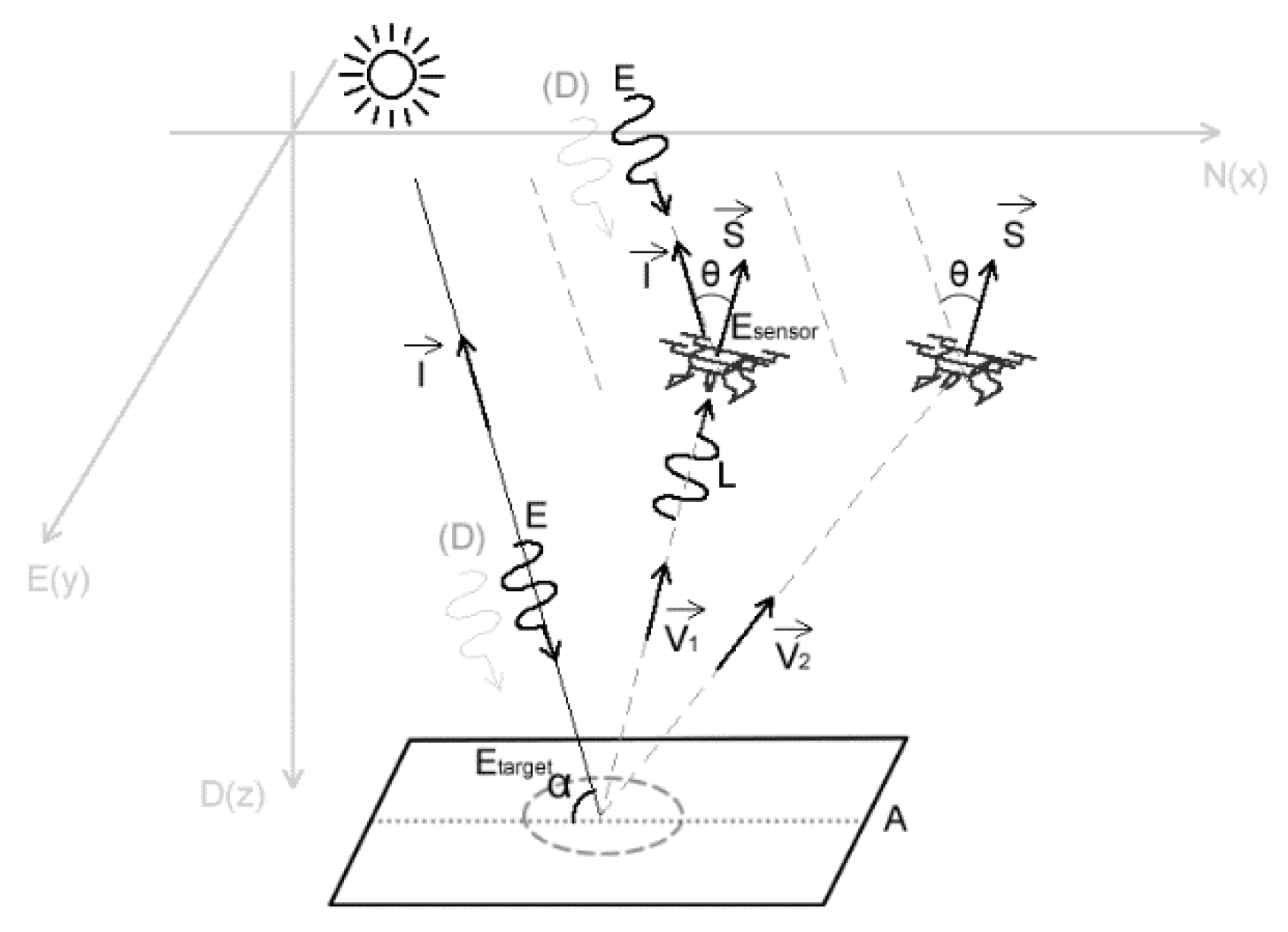
For the first sub-module of variables retrieval, the dependent variable (R) is calculated within the framework of RedEdge radiometric calibration applications. This is the bidirectional reflectance factor, defined as the ratio of the radiant flux reflected by a target surface to the radiant flux from an ideal diffusive surface of the identical geometry [9]. Illustrated by Figure 3, the reflectance factor (R) of an infinitesimal surface (A) under incoming radiance (Etarget) from any view direction () is expressed by Equation (2). For reading convenience, the proof of involving RedEdge computed at-sensor-radiance (L) and at target irradiance (Etarget) in this equation is attached in Appendix A.
where:
- R—the observed reflectance factor;
- L—at-sensor-radiance (W/m2);
- Etarget—the irradiance (W/m2) at the target surface A;
- —the BRDF that takes the parameters of incoming zenith and azimuth θi, φi, and view zenith and azimuth θv, φv. To reduce one degree of freedom, the function is normally written as , where φ is the relative azimuth of φv counterclockwise rotated from φi. Here, this function is the Walthall model in Equation (1).
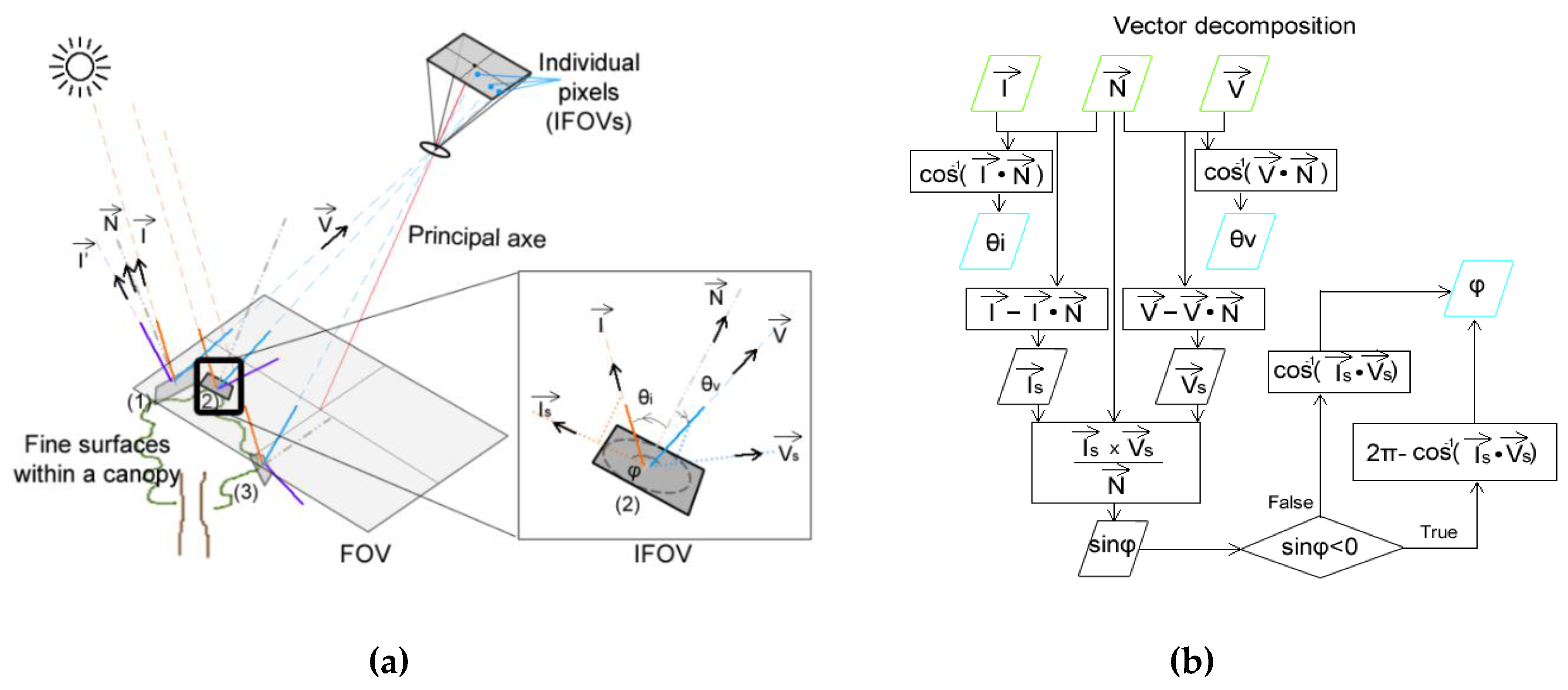
The second sub-module retrieves the geometric variables at the fine optical level. Within an FOV as illustrated by Figure 4a, an individual sun-target-sensor geometry can be established for each instantaneous field of view (IFOV), or pixel. This pixel depicts a “fine” surface section from a canopy. Corresponding to a directional reflectance value, the geometry contains three vectors: a solar incident vector , a surface normal vector that describes the “fine” surface, and a view vector that describes the viewing angle of the pixel.
Given the three vectors, the geometric parameters required by the Walthall model can be easily decomposed as illustrated by the workflow in Figure 4b.
As the first element of the three vectors, unit solar incident () data cubes are computed. When provided with GPS and timestamp of one image, a unit solar incident can be computed in the north-east-down (NED) coordinate system by PySolar packages [33]. The vector is then rotated back to the RedEdge image perspective coordinates by the image exterior orientations latter computed from Metashape. For each pixel within an image, is the same.
For the second element, the 3D reconstruction workflow of Metashape was implemented to compute a surface model. A typical workflow generally consists of the following steps:
- A robust scale-invariant feature and match detection on image pairs. In this case, the direct reflectance images were used, and the RedEdge band was used as the master-band, due to its vegetation sensitivity.
- A sparse point cloud generation that computes the robust matching features in the 3D coordinates and aligns the camera extrinsic via structure from motion (SfM) methods.
- Depth maps generation on fine elements (on a downscaling of four pixels) by stereo pairs.
- A dense point cloud generation that computes the fine elements on the 3D coordinates based on their depth.
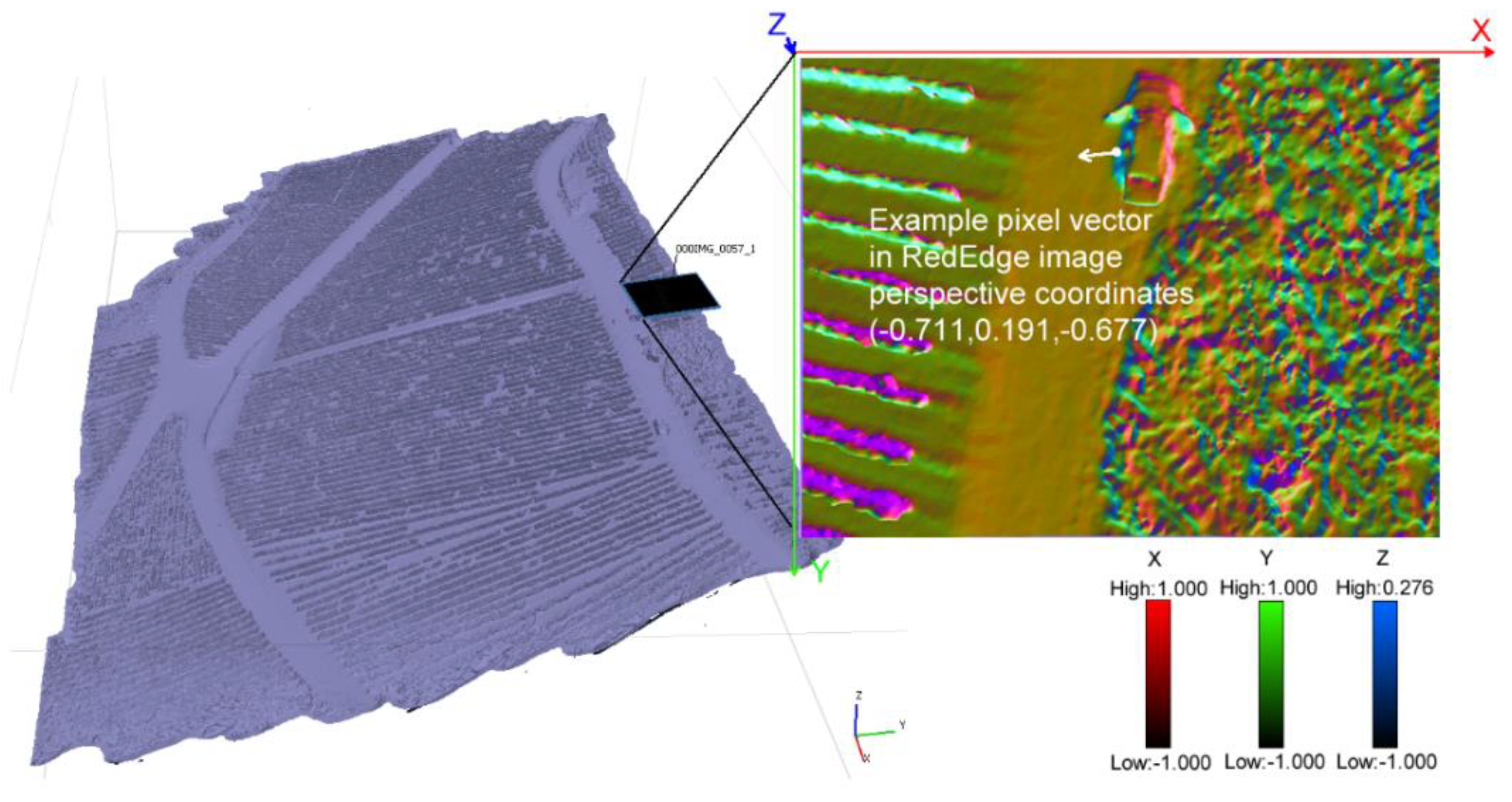
- Since the dense points do not have the image resolution, the mesh generation triangular irregular network (TIN) interpolates the dense points to the pixel level in the 3D coordinates to fill the gaps. In Figure 5, this mesh is visually described by the TIN faces (the violet 3D surface map on the left and the colorful micro triangle surfaces on the right) and numerically described by the unit surface normal vectors.
- Rendered by the FOVs from the mesh, the data cubes for all the images are thus reached.
Illustrated in Figure 6, the remaining view vector from a pixel (x, y) to the focal point (O) within the RedEdge image perspective coordinates is defined by Equation (3), which needs to be scaled to a unit vector afterward. The view vector is computed from an undistorted image, where travels in a straight line. For one camera (i.e., red or NIR), the data cube is always the same in the image perspective coordinates, which is determined by the camera intrinsics.
where:
- (x, y)—the location of the pixel in RedEdge image perspective coordinates;
- (x0, y0)—the location of the principal point in RedEdge image perspective coordinates computed from Metashape;
- p—the pixel size;
- f—the focal length of each camera.
When computing all the vectors of interest under the RedEdge image perspective coordinates, the procedure favored the optical parameters (e.g., principal point location and distortion parameters) and camera exterior orientation computed by Metashape. The reason is that vector geometries between 3D and 2D should be as aligned as possible, where optimized intrinsic and extrinsic are preferred over the original ones. Also, since the gimbal did not carry an inertial measurement unit (IMU), camera exterior orientations had to be computed by Metashape.
2.2.2. BRDF Sampling
After computing the necessary variables, every single pixel became a possible BRDF study object. Nine hundred and seventy-two camera shots in one flight made over one billion pixels (972 shots * 960 rows * 1280 columns) available for anisotropy study, which was a very large dataset.
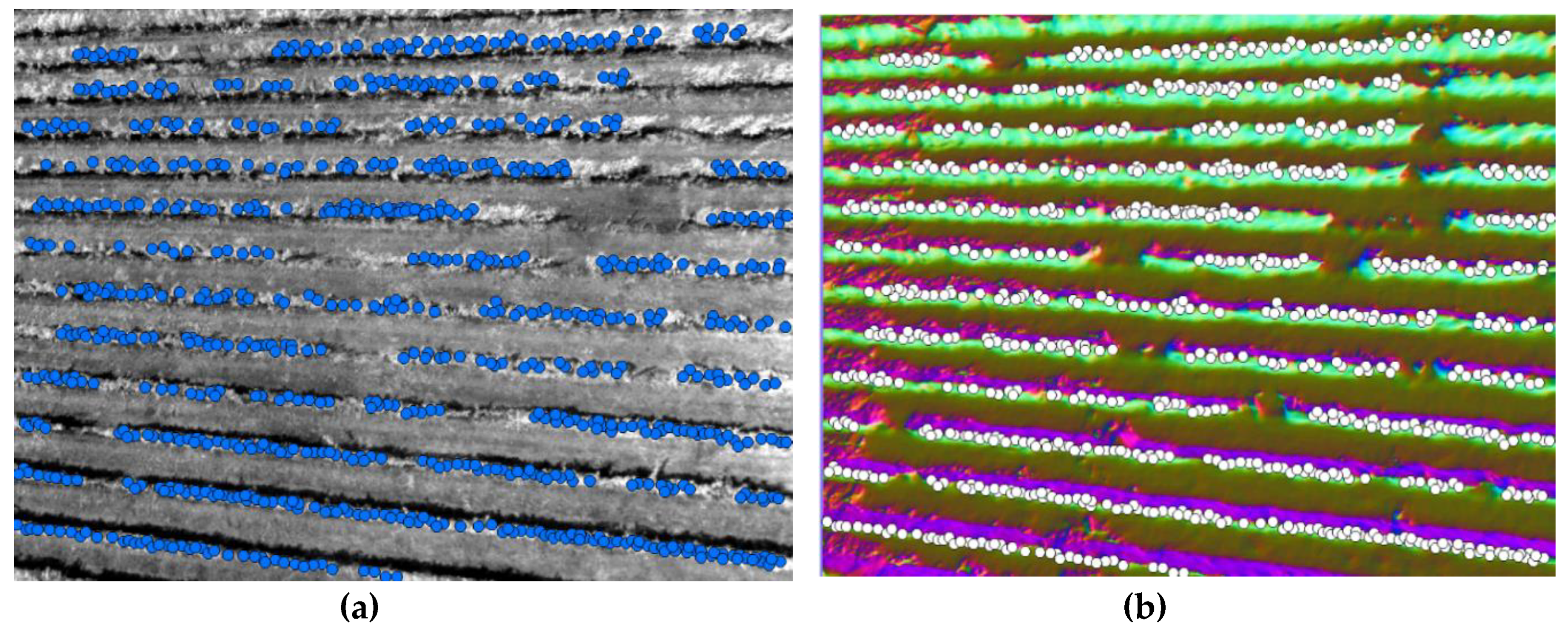
For sampling, this study narrowed down to red and near-infrared (NIR) bands for NDVI analysis. Large quantities of points were manually allocated to the reflectance–normal image pairs (Figure 7). With the assistance of normal maps, the manual sampling has the following visual criteria: (1) a point falls on a vine canopy; (2) that canopy has not been affected by disease or drought or is severely shadowed (most representative for the study area canopy majority); (3) the geometries of points should be as diverse as possible (to ensure the anisotropy variety).
Six images were selected for both red and NIR bands as the training dataset. Then, 4856 points were sampled for red, and 3386 points were sampled for NIR. Three images were selected as the validation dataset, with 1390 points sampled for red, and 1373 for NIR. The difference in point number was due to the manual points allocation, where “confident sampling” differed from the human judgment on the individual image of each band.
To sample the directional reflectance, a 3 x 3 pixel window was center-located at a point and took the average value from this window. To sample the geometric variables, the points directly took the pixel values that were decomposed from the three-image vector-data cubes (, , and ) via the method described in Figure 4b. The reason for this sampling method is that the computed normal map is spatially continuous, while the direct reflectance image representing the real world is not; thus, it needs to be kernel smoothed.
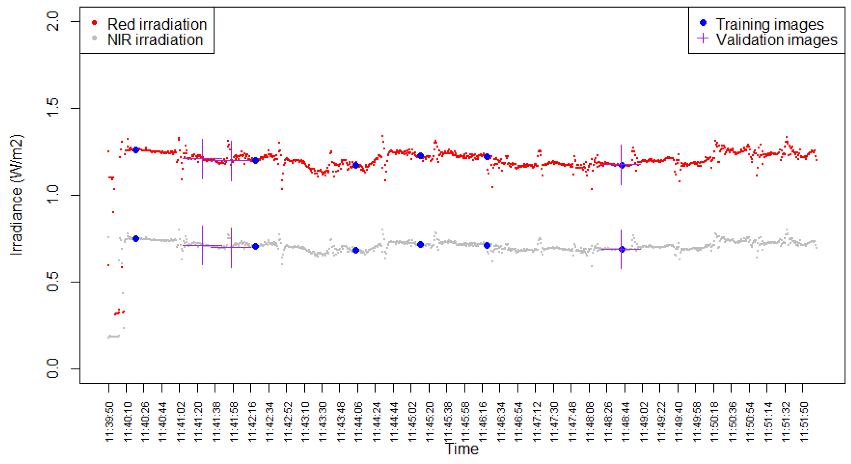
The training and validation images were evenly distributed during the flight (Figure 8), without a sudden change of sunlight.
2.2.3. BRDF Modeling and Correction
After sampling, the three geometric variables θi, θv, and φ, along with the R from the training dataset, were imported into the Walthall model in Equation (1), as multilinear regression, to empirically determine the four coefficients.
2.3. Result Analysis
2.3.1. Sample and Model Visualization
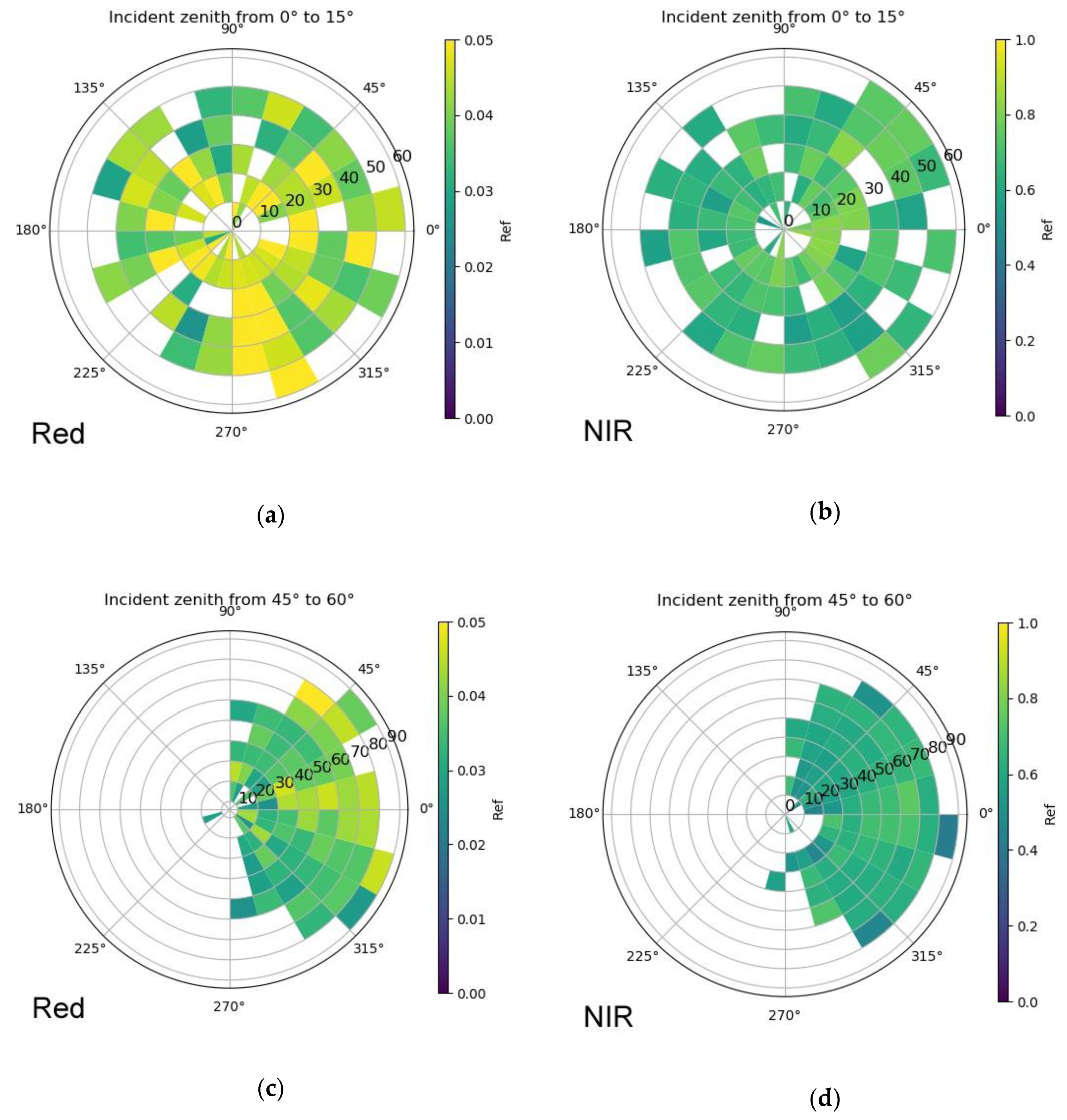
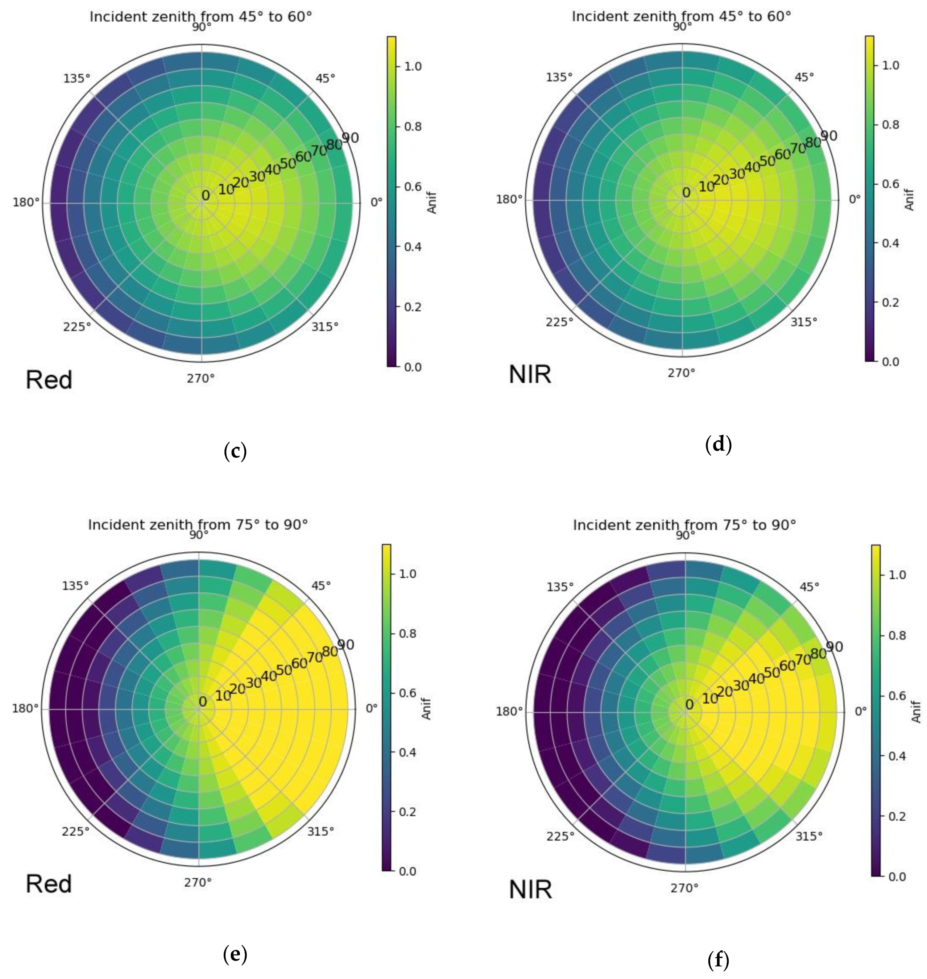
First, the results of BRDF sampling and modeling were illustrated in the polar plots of six incident zenith classes. The anisotropy was classified into 1296 angle classes (6 incident zenith x 24 relative azimuth x 9 view zenith).
The values that fell in every incident zenith range class were displayed on a single polar plot, where the incident light comes from the azimuth 0° (right) and an incident zenith range is shown on the subtitle. On this plot, the view zenith increases outward from the center (each circle is 10°), and the relative azimuth increases counterclockwise from the right (each grid is 15°). Due to the fine angular resolution, a grid displays only the median of the corresponding values within an angle class.
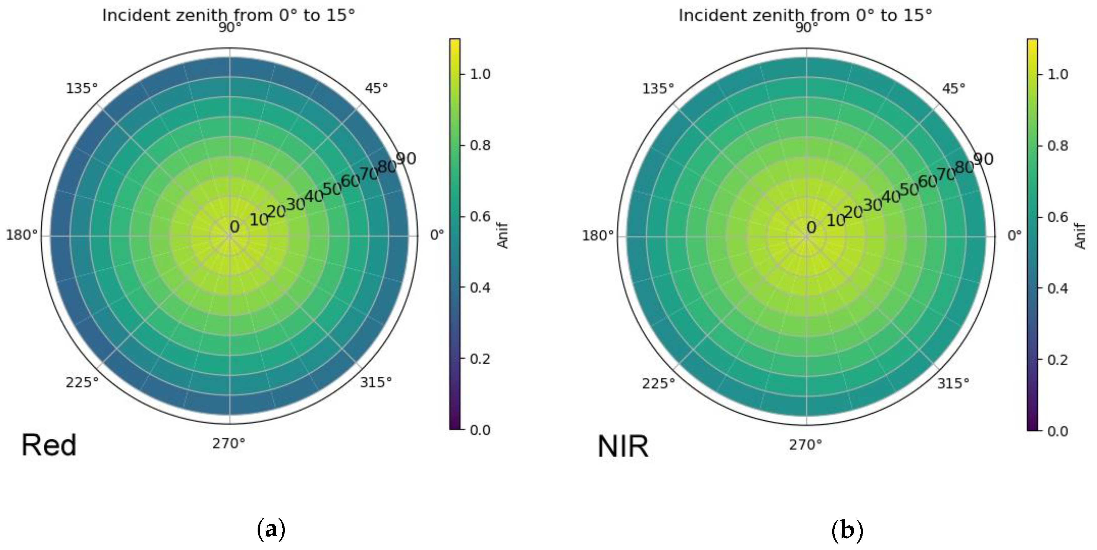
The sampling was illustrated by the reflectance, while the modeling result was illustrated by the anisotropy factor anif = for literature comparison.
2.3.2. Prediction Assessment on Validation Points
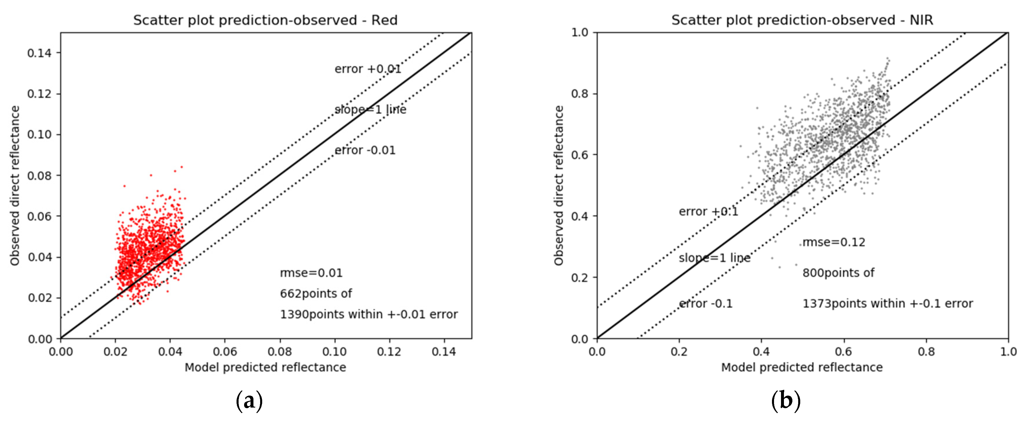
After the polar visualization of the trained models, the prediction accuracy was assessed by the validation points. Due to the vegetation sensitivity difference in red and NIR bands, the vine canopy reflectance varied in significantly different ranges (red 0.01~0.04, NIR 0.6~0.8). To analyze the accuracy in a similar scope, root-relative square errors (RRSEs) were first computed between the predicted and observed reflectance, along with RMSEs on the validation points. A result close to 0 indicates good performance.
Then the observed and predicted reflectance was scatter plotted for the validation points. A converged shape of points on slope = 1 indicates an ideal prediction. Due to the large number of values and the canopy complexity, a certain level of errors was unavoidable. Therefore, reflectance error threshold lines were arranged beside the slope = 1. They were set as ±0.01 for the red band and ±0.1 for the NIR, which make the common spectral error range for vegetation remote sensing.
2.3.3. Correction Assessment on Validation Points
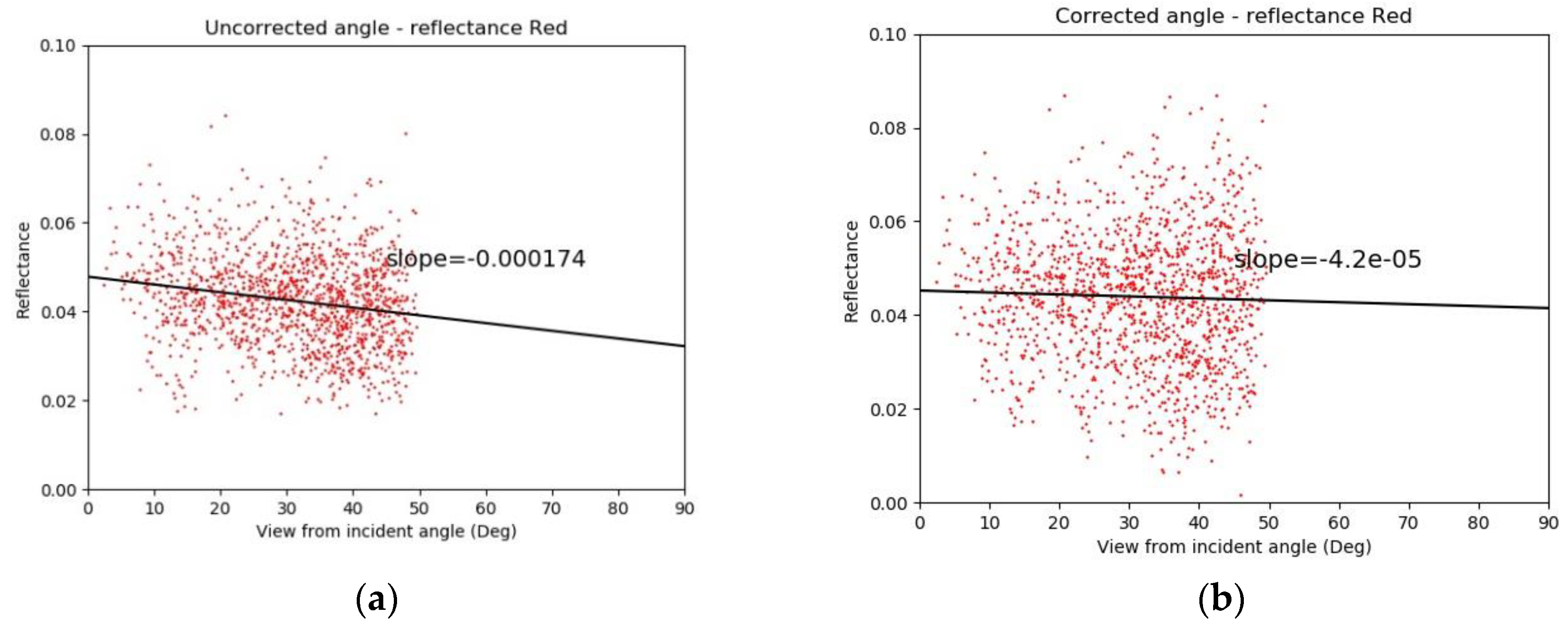
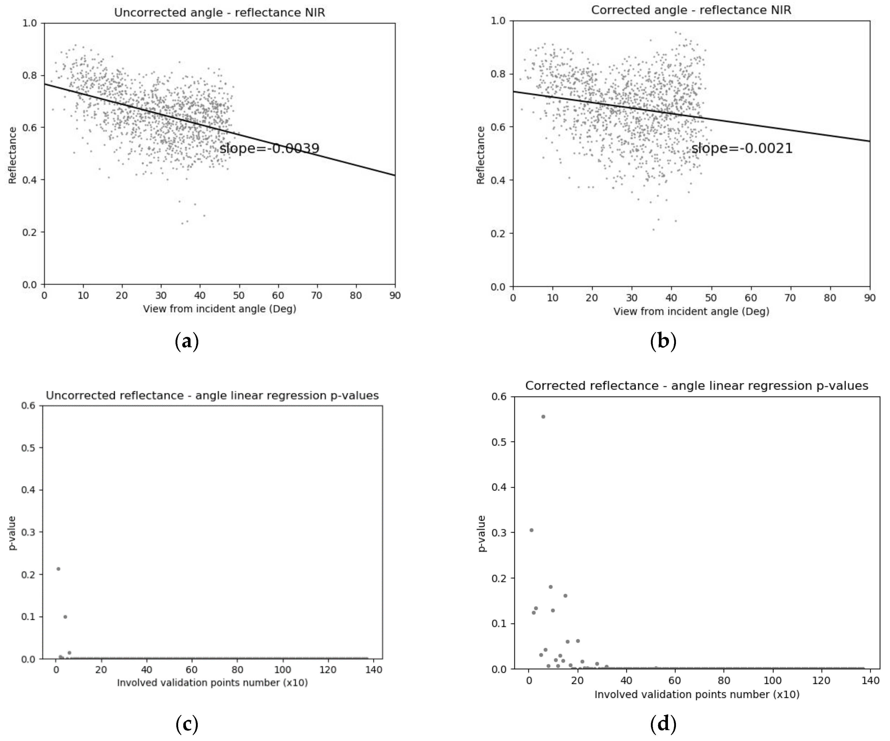
After angular correction, the performance was first assessed on the validation points. Based on the results of modeling, the backscattering effect dominated the vine canopy directional reflectance, where the reflectance increases by the decreasing view-incident angle. To illustrate this angular dependency and the independency after correction, reflectance and view-incident angles were scatter plotted for the validation points, without considering the surface normal (for 2D plot illustration simplification).
Again, due to the large quantities of points, a single p-value from reflectance-angle linear regression always tends to be significant. Therefore, a p-series analysis was conducted. An increasing number of points (once every +10 points) were randomly pair-selected from both corrected and uncorrected validation points, where a p-value for the reflectance-angle regression was separately computed. Then the p-values were plotted against the number of the points involved in the regression. In this pair, the later the low p-value appears in the correction series, the more successfully the angular correction performs.
2.3.4. Correction Assessment on NDVI Orthomosaics
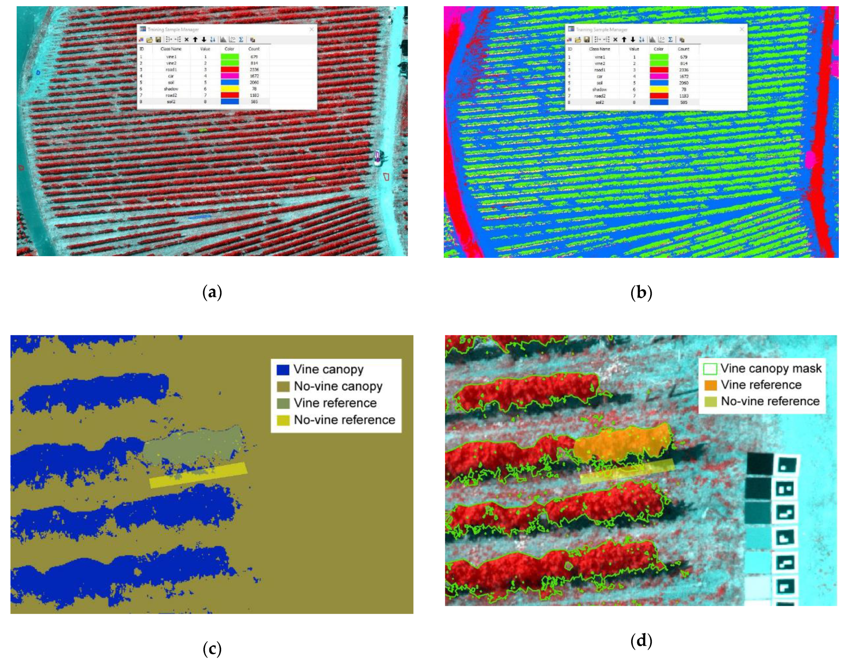
Both corrected and uncorrected orthomosaics were computed from two different view directions. Since the angular correction was uniformly performed on all pixels, all non-vine pixels were “corrected” in the final orthomosaics. To focus on the vine canopies, a supervised maximum likelihood classification in ArcGIS was implemented on the uncorrected orthomosaic to form an effective canopy mask first.
The classification steps are: (1) major thematic class mask selection (vine, soil, shadow, car, etc.) on an orthomosaic in Figure 9a; (2) inputting the 5 bands’ spectral signature of these masks to the algorithm for classifier training; (3) applying the classifier on the whole orthomosaic to form the class-map in Figure 9b; (4) converting the class map to a binary mask for vine and non-vine canopy in Figure 9c.
The method yielded an acceptable canopy mask. For instance, in Figure 9c,d, the two user-defined references concluded that 2976 out of 3046 pixels were correct in a vine reference, and 1173 out of 1342 pixels were correct in a no-vine reference. The kappa statistics was therefore 86.9%, yielding satisfying accuracy. In Figure 9d’s direct illustration, the only false classified targets are the dense grasses that stand very close to the vine canopy bottom.
On each view direction, the canopy mask retrieved the red and NIR data cube from both the corrected and uncorrected orthomosaics, resulting in 4 NDVI maps (uncorrected vs corrected on 2 different angles). Four boxes were put on four canopy rows to extract values from these NDVI maps. The median value differentials between the two directions were computed on each box for both the uncorrected and corrected. This was also computed for all the pixels in the NDVI maps. The median differential from the corrected should be smaller than the uncorrected, due to angular independence.
3. Results
3.1. Sample and Model Visualization
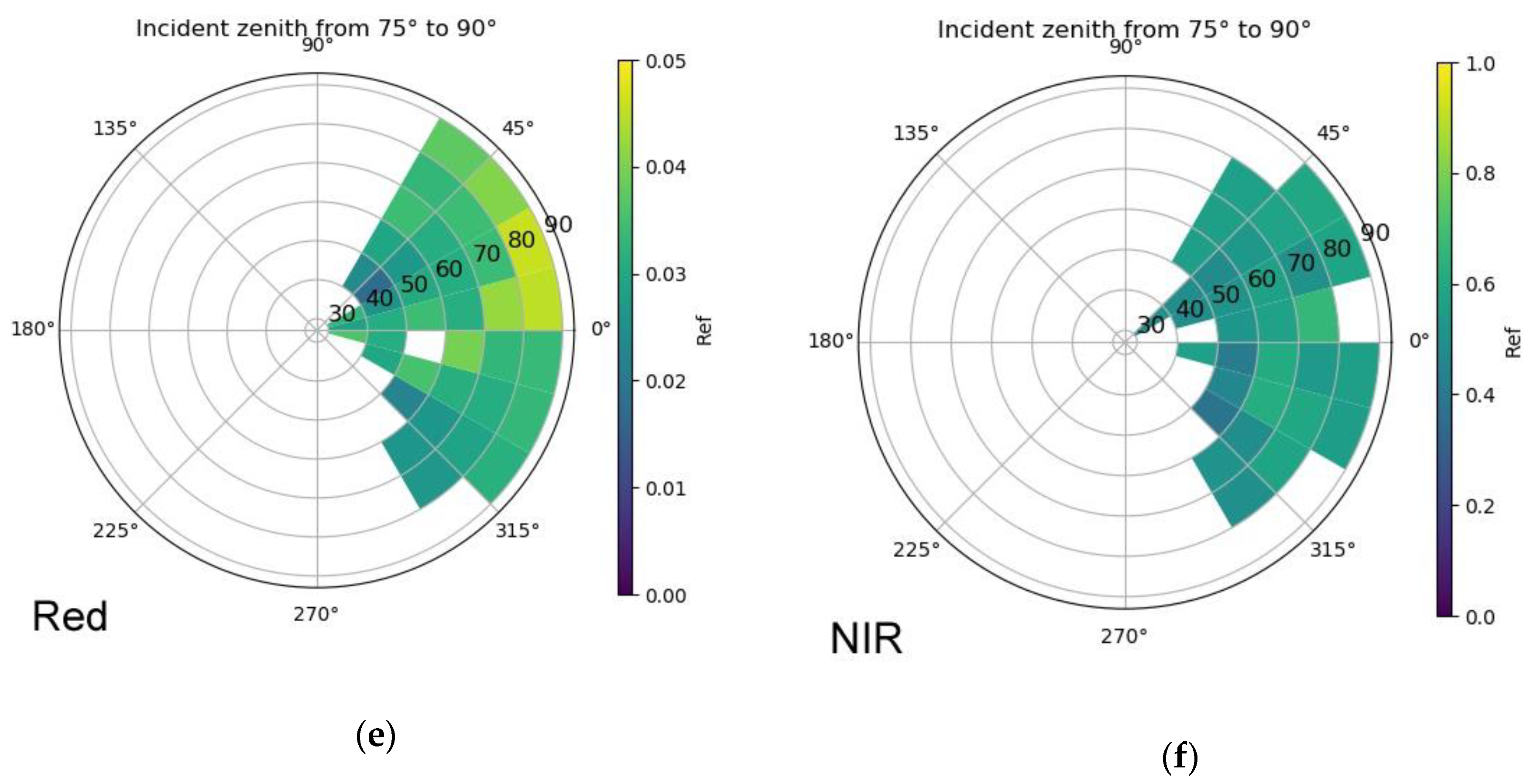
Figure 10 shows that the sampled reflectance of three incident range classes for both the red and NIR bands. Generally, the angular dependency has similar patterns for red and NIR reflectance, with brighter backscattering reflectance and darker forward-scattering. The brightness is most pronounced in the small incident zenith backscattering direction (Figure 10a,b).
As the incident angle increased, the number of reflectance samples in the forward-scattering (the left part in a polar plot) decreased.
Figure 11 illustrates the anisotropy factor development from low to high sun incident zenith for red and NIR bands. Both bands showed backscattering effects, with the increasing anisotropy factor toward the solar incident direction. The red anisotropy factor spread wider than NIR in the large incident zenith.
3.2. Prediction Assessment on Validation Points
As illustrated by Table 2 and Table 3, although the NIR RMSE was larger than the red, the RRSE suggests that NIR model prediction was comparatively better than the red model, when values were standardized by the original observations.
Illustrated by Figure 12a, 47.63% of the red points were accurately predicted within ±0.01 prediction errors. In Figure 12b, 58.27% of the NIR points were accurate within ±0.1 prediction errors. This proved the RRSE statement before.
The R2 of prediction to observation upon slope = 1 is –1.01 for red and –0.36 for NIR, expressing no linearity in both cases. Excluding the points that are outside of the error ranges, the R2 is increased to 0.41 for red and to 0.52 for NIR.
Judged from the observation–prediction point distribution, underestimations are observed in both red and NIR predictions.
3.3. Correction Assessment on Validation Points
In Figure 13, the reflectance-angle slope is flattened after angular correction. The p-series analysis suggests that the red reflectance is completely angular independent for the corrected validation points.
Similarly, in Figure 14, the reflectance-angle slope has also been flattened, but there is still a very low-level linear relation. Also, after involving more than 210 validation points, the significance of the angular dependency showed up again. This indicates that the angular effect was not completely removed from the NIR band.
The anisotropy correction factor in Figure 15c illustrates the spatial distribution of correction factors when the model was image-wise applied to all the canopy pixels.
For the canopy reflectance in this image, 15.9% of the pixels are reduced by more than 10%, while 13.3% of them are increased by more than 10%, and the majority of correction factors are around 1 (no change). The decreased reflectance pixels (purple) locate in the upper and bottom edges; the increased (red) are mainly in the right bottom corner, and the unchanged (cyan) dominate the central left down.
3.4. Correction Assessment on NDVI Orthomosaics
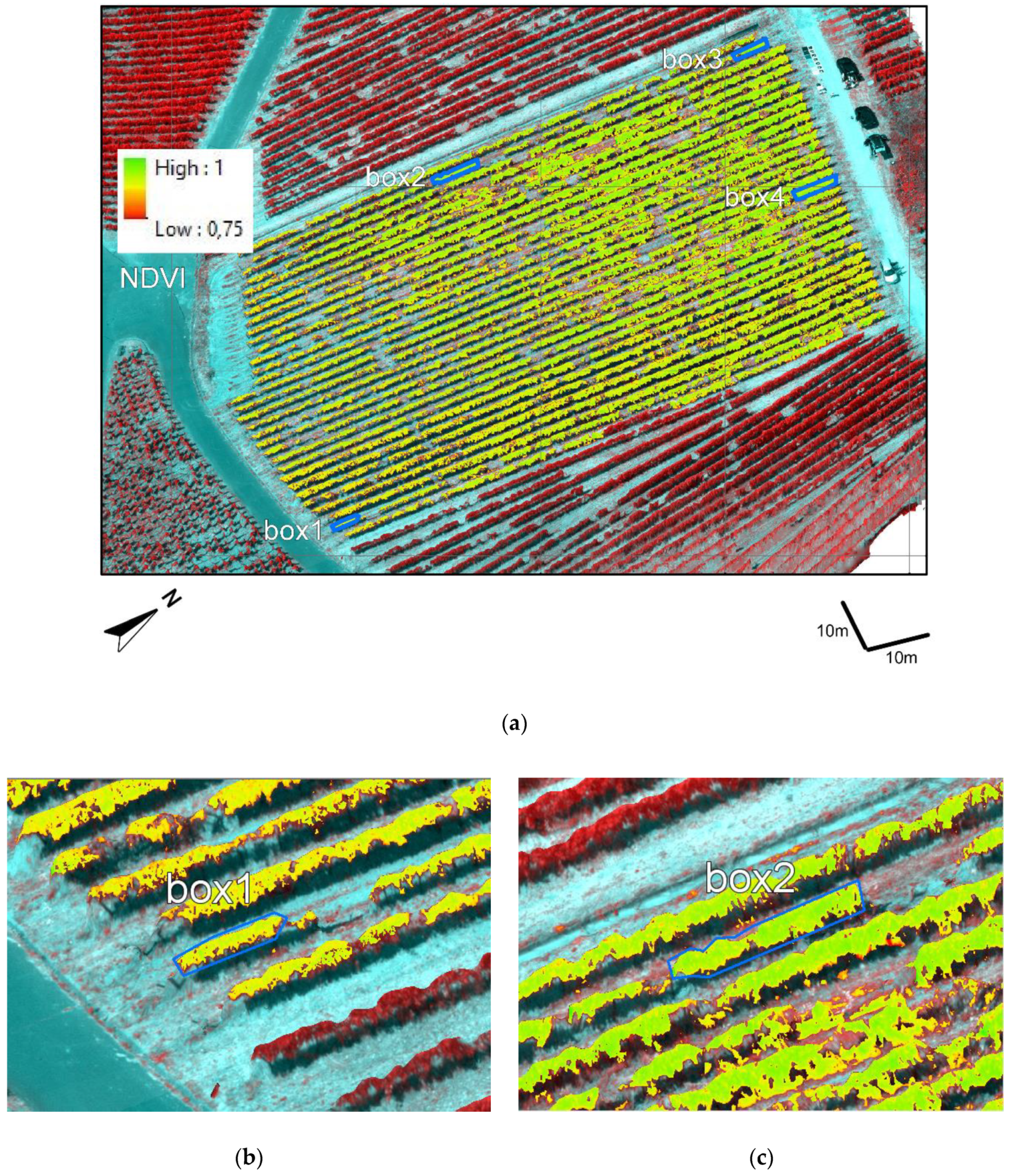
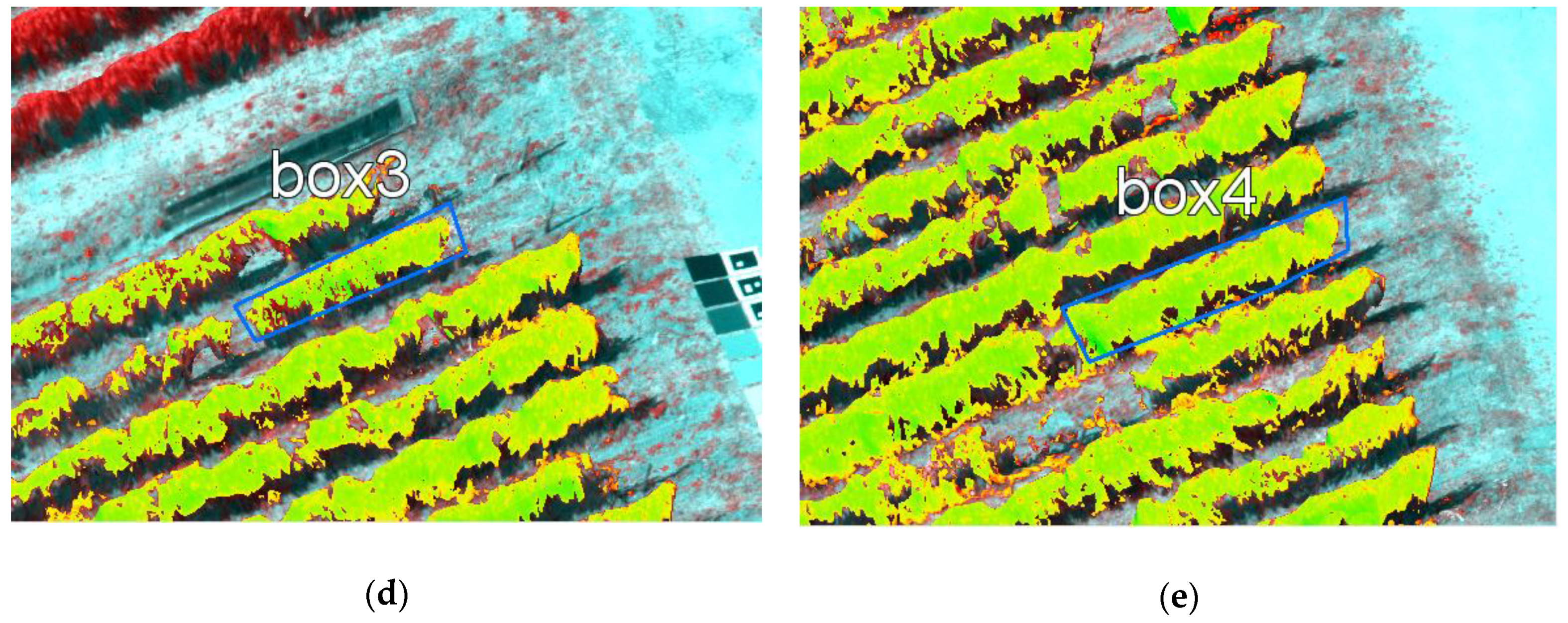
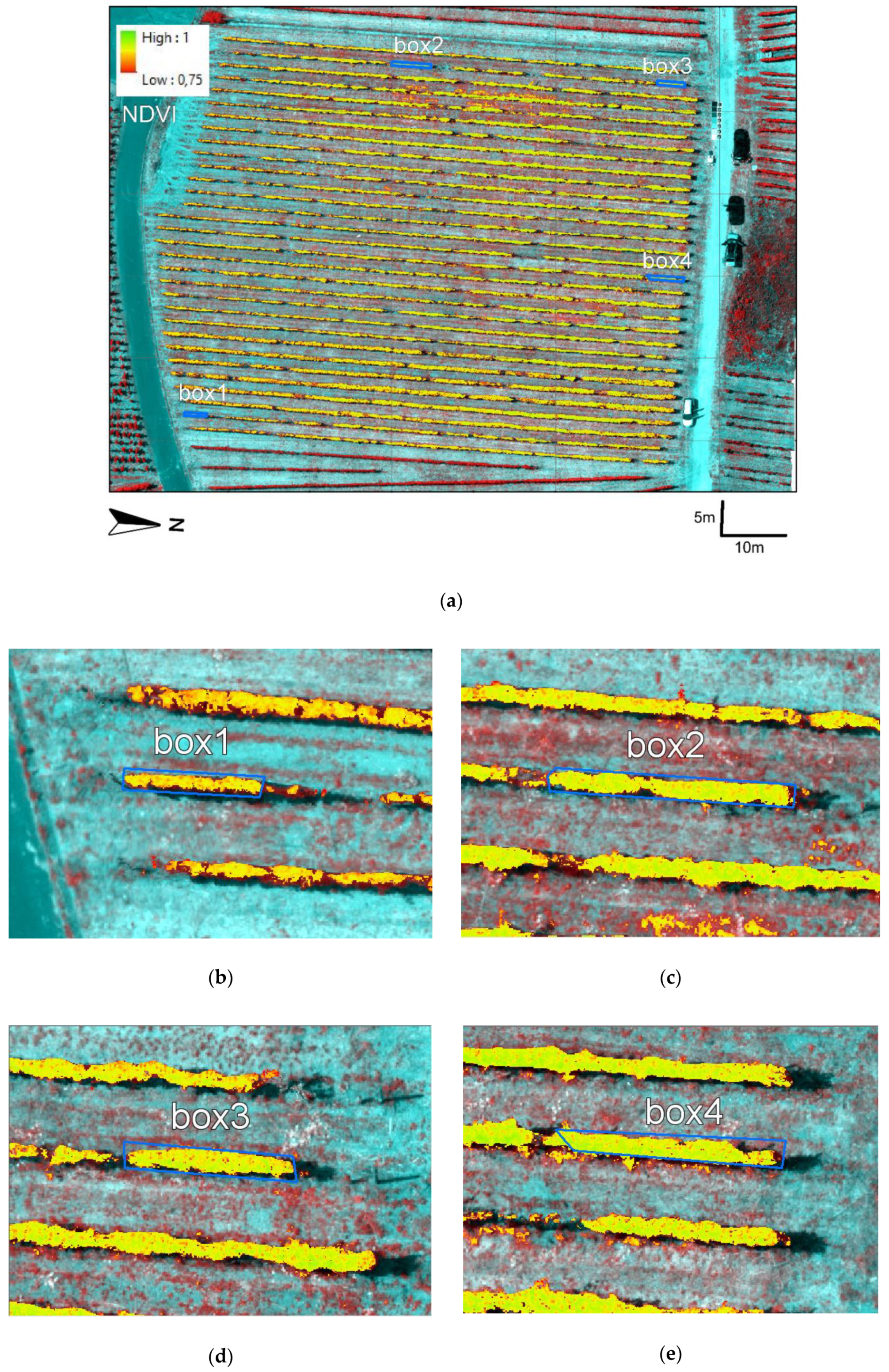
Figure 16 and Figure 17 illustrate the corrected NDVI orthomosaics from two different viewing directions in locally defined coordinate systems, with the canopy row boxes displayed on the zoomed-in images. Compared with the first direction, the second direction was closer to nadir. Aside from the shape, the depicting canopy section sizes (pixel number) are also different. Canopy-viewing sections from the first direction are larger than those in the second.
The medians of the directional NDVI differentials are summarized in Table 4. The uncorrected directional NDVIs were actually smaller in Box 3, Box4, and also the whole NDVI map.
4. Discussion
The proposed procedure was evaluated by the sample- and model-result visualization, the prediction and correction assessment on validation points, and finally the correction performance assessment on NDVI orthomosaics.
In Figure 10c–f, no forward-scattering reflectance could be sampled when incident zenith was large. This was limited by the actual flight scenario. For instance, when the high sun elevation and steep canopy surface formed a large incident angle on the fine surface (3) illustrated in Figure 3, the forward directions were downward; thus, they could not be captured by the UAV mounted camera.
The model visualization in Figure 11 has yielded expected results. Figure 11c has a similar pattern as illustrated by an RPV model simulated red reflectance on black spruce [9] under incident sun zenith 30°. Figure 11e,f also shares similar patterns with the Walthall model derived anisotropy on winter wheat, under incident sun zenith 39.8° [26]. This proves the procedure’s functionality at the methodology level.
As for the prediction, this study reached 0.64 and 0.52 (red R2 = 0.41 and NIR R2 = 0.52) for vine canopy, when excluding the points out of the accepting error ranges. Compared with the high correlation coefficients (0.87~0.94 for red, 0.83~0.93 for NIR) on a spectralon [23] obtained under a clear sky, there is a limitation. Nevertheless, given the complexity of a canopy and the amounts of the points, the results showed a reasonable level of prediction accuracy.
For both the red and NIR bands, a certain level of underestimation was observed. The most likely explanation is the micro shadow variation involved in the training procedure. One of the major advantages of high-resolution UAV images is the canopy structure details, but this also enlarges the observable heterogeneity where the tiny shadow variations are visible on the image. Therefore, the training data could include directional reflectance that was affected by the shadows. In the red band, the major absorption in the wavelength reduced the vegetation red reflectance to a very low scope, leading to the confusion between real vegetation reflectance and shadows. Meanwhile, this problem was further complicated by the high reflectance-vegetation sensitivity in the NIR. The hidden layer beneath the canopy surface that increased NIR reflectance, which could not be distinguished by a feature-detection-based 3D computation, was further combined with this micro-shadow effect. In short, when variant reflectance was corresponding to the same geometries, errors were produced. Indeed, the vegetation detail features, such as LAI, can have major impacts on the canopy bidirectional effect, as other studies have shown [22,23].
Another possible limitation is from the 3D surface model, which causes the inaccuracy of inputting geometric variables. Although this can be improved by computing the dense points of higher resolution, the time cost will be increased. Also, the detail of the computable dense points is limited by the detectable contrast in an image, which is namely linked with the vegetation sensitivity of the sensor itself.
Accordingly, it was also proved on the validation points that the angular dependency is removed from red and partially removed from NIR.
However, when magnifying from points to map level, the hypothesis could not be completely proved on the NDVI orthomosaics. It was originally assumed that the procedure could correct the angular dependency at fine resolution level purely from the canopy out-surface structures, yet the changing view directions also corresponded to the changing of relative canopy features to the sensor, such as hidden layer thickness and leaf orientation. The variation of these unknown features, combined together with micro shadows, could have frustrated the results.
There are several points in this procedure that could be proved. The first is the sampling procedure. Instead of the human selection on the individual bands, a highly accurate band-alignment algorithm could help the retrieval of sampling points from the same real-world location for each band. Also, an NDVI mask could be created on this alignment to assist the point sampling, avoiding the micro shadows to a certain scope. Further image-based methods to derive more detailed vine canopy features (LAI, leaf orientation, etc.) with other BRDF modeling tools are expected to improve the functionalities.
5. Conclusions
This paper has illustrated an example workflow for a tilted MicaSense© RedEdge-M multispectral sensor to sample, model, and correct the vine canopy angular reflectance in a sloped area.
This method utilized the sensor’s own radiometric package to derive the directional reflectance, computed the canopy out-surface geometries by Agisoft© Metashape, and empirically established the Walthall BRDF model.
The study showed that such methods could sample and model the angular dependency without ground measurements. The validation points showed that an empirically established model could achieve prediction accuracy to RRSE 1.42 in the red band and to RRSE 1.17 in the NIR band. This means the procedure can be useful for modeling bidirectional reflectance captured by this sensor under any other circumstances.
The correction showed certain effectiveness on validation points, but could not on NDVI orthomosaics. This indicates that the proposed procedure can function on a coarser resolution, but cannot be applied on a fine-resolution orthomosaics for inhomogeneous vegetation such as vine canopies.
Author Contributions
All authors provided editorial advice and participated in the review process; R.R. and T.U. conceived of and designed the project experiments; conceptualization, methodology, and results interpretation by C.G., H.B., and T.U.; data curation by R.R.; and T.U. led the research group.
Acknowledgments
The experiment was designed in cooperation with Matthias Porten (DLR Mosel, Dep. Of Viticulture and Enology), who provided the test site and grape assessments, together with Christopher Hermes. UAV configuration (including sensor) and flight were carried out by Freimut Stefan (DLR Mosel). The publication was funded by the Open-Access Fund of Universität Trier and the German Research Foundation (DFG) within the Open-Access Publishing funding program.
Conflicts of Interest
The authors declare no conflicts of interest.
Appendix A
To compute the raw image pixel value to absolute spectral at-sensor-radiance (L) in units of W/m2, the RedEdge radiometric model is used [35].
where:
- L—absolute spectral radiance for the pixel (W/m2) at a given wavelength;
- V(x,y)—pixel-wise vignette correction function, see (Equation (A4));
- a1, a2, a3—RedEdge calibrated radiometric coefficients;
- te—image exposure time;
- g—sensor gain;
- x,y—the pixel column and row number;
- p—normalized raw pixel value;
- pBL—normalized black level value, attached in image metadata
The vignette correction function V(x,y) is defined by Equation (A2):
where:
- r—the distance of the pixel from the vignette center;
- cx,cy—vignette center location;
- k—a vignette polynomial function of 6 freedom degrees [36];
- k0, k1, k2, k3, k4, and k5—the MicaSense calibrated vignette coefficients.
To rotate any vector in the RedEdge-M image perspective coordinates to world north-east-down (NED) coordinates, as illustrated in Figure 6, the following rotation matrix is used:
where:
- —a vector in real-world NED coordinates;
- —a vector in image perspective coordinates;
- α—the roll angle;
- β—the pitch angle;
- γ—the yaw angle;
- R—the overall rotation matrix.
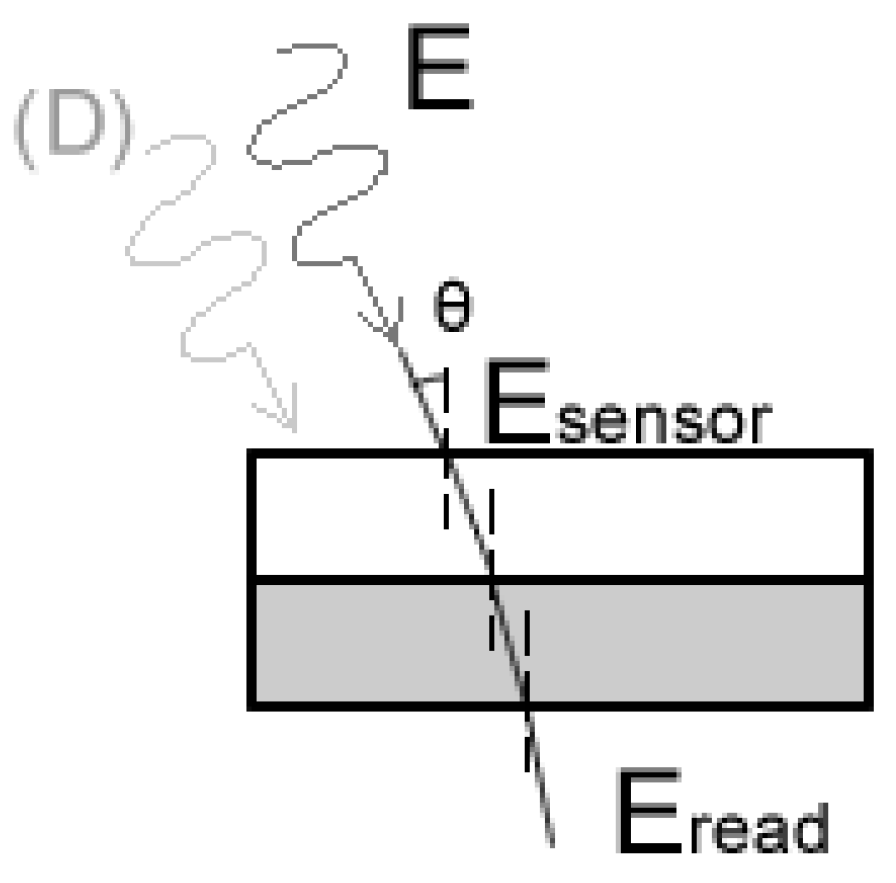
When the DLS is upward configured in the UAV, its directional vector in the RedEdge image perspective coordinate is (0,0,–1). It is rotated into the real world NED coordinate . As illustrated by Figure 3, the θ between the incident sun vector () and DLS direction () can be thus computed by the arccosine of .
As stated by the Fresnel equations, the transmittance of an individual media (mi (i = 1,2,3)) in the multilayer DLS sensor is defined by the Equation (A6). In this equation, the fractions of s and p polarization reflection are both assumed to be ½. The fractions are calculated by Equations (A7) and (A8). Starting by the sun-DLS sensor zenith as the initial incident zenith, the transmissivity of each layer is iteratively computed by the exiting layer zenith (θi) and the current layer media refractive index (ni). The incident angle (θi+1) for the next media is determined by the Snell’s law ni = ni+1 , where the final transmittance is the accumulated transmittance multiplication product of all the layers in Equation (A9).
where:
- —the s-polarized reflectance of the media mi;
- —the p-polarized reflectance of the media mi;
- —the incident zenith on the media mi;
- —the refractive index of the media mi;
- —the transmissivity of media mi, when the fractions of reflectance are both assumed ½;
- —the overall transmissivity of the multilayer DLS receiver of 3 layers.
Figure A1.
The DLS transmissivity

By reaching the overall transmittance, the irradiance at the top of the DLS sensor is Esensor = Eread/T. Assuming an isotropic atmospheric diffusive compartment of 1/6 is added to the direct incoming radiance beam under clear weather conditions, the global incident radiance in the study area at that moment is computed as E = Esensor/(cosθ + 1/6), where θ is the zenith of sun incident on DLS sensor. As illustrated by Figure 3, the incoming radiance at target Etarget = E(sinα + 1/6), where α is the solar altitude on a flat surface.
Illustrated by the literature [9] case 1, the bidirectional reflectance factor is defined by the ratio of the reflected radiant flux to the reflected radiant flux from an ideal diffuse surface under identical view geometry by Equation (A10). Expanding the flux to cosine radiance multiplied by the solid angle on the area dA as Equation (A11), terms can be simplified as Equation (A12). Since the ideal diffusive reflectance is 1/π, Equation (A13) is finally reached, where and can be sampled by the at-sensor-radiance (L) and at-target-irradiance (Etarget) explained above, proving Equation (2).
References
- Arnó, J.; Martínez-Casasnovas, J.A.; Ribes-Dasi, M.; Rosell, J.R. Review. Precision Viticulture. Research topics, challenges and opportunities in site-specific vineyard management. Span. J. Agric. Res. 2009, 7, 779–790. [Google Scholar]
- Weiss, M.; Baret, F. Using 3D Point Clouds Derived from UAV RGB Imagery to Describe Vineyard 3D Macro-Structure. Remote Sens. 2017, 9, 111. [Google Scholar] [CrossRef]
- De Castro, A.I.; Jiménez-Brenes, F.M.; Torres-Sánchez, J.; Peña, J.M.; Borra-Serrano, I.; López-Granados, F. 3-D Characterization of Vineyards Using a Novel UAV Imagery-Based OBIA Procedure for Precision Viticulture Applications. Remote Sens. 2018, 10, 584. [Google Scholar] [CrossRef]
- Zarco-Tejada, P.J.; Berjón, A.; López-Lozano, R.; Miller, J.R.; Martín, P.; Cachorro, V.; González, M.R.; De Frutos, A. Assessing vineyard condition with hyperspectral indices: Leaf and canopy reflectance simulation in a row-structured discontinuous canopy. Remote Sens. Environ. 2005, 99, 271–287. [Google Scholar] [CrossRef]
- Matese, A.; Di Gennaro, S.F. Practical Applications of a Multisensor UAV Platform Based on Multispectral, Thermal and RGB High Resolution Images in Precision Viticulture. Remote Sens. 2018, 8, 116. [Google Scholar] [CrossRef]
- Romero, M.; Luo, Y.; Su, B.; Fuentes, S. Vineyard water status estimation using multispectral imagery from an UAV platform and machine learning algorithms for irrigation scheduling management. Comput. Electron. Agric. 2018, 147, 109–117. [Google Scholar] [CrossRef]
- Burkart, A.; Aasen, H.; Fryskowska, A.; Alonso, L.; Menz, G.; Bareth, G.; Rascher, R. Angular Dependency of Hyperspectral Measurements over Wheat Characterized by a Novel UAV Based Goniometer. Remote Sens. 2015, 7, 725–746. [Google Scholar] [CrossRef] [Green Version]
- Aasen, H. Influence of the viewing geometry within hyperspectral images retrieved from UAV snapshot cameras. ISPRS Ann. Photogramm. Remote Sens. Spat. Inf. Sci. 2016, 3, 257. [Google Scholar] [CrossRef]
- Schapeman-Strub, G.; Schapeman, M.E.; Painter, T.H.; Dangel, S.; Martonchik, J.V. Reflectance quantities in optical remote sensing-definitions and case studies. Remote Sens. Environ. 2006, 103, 27–42. [Google Scholar] [CrossRef]
- Walthall, C.L.; Norman, J.M.; Welles, J.M.; Campbell, G.; Blad, B.L. Simple equation to approximate the bidirectional reflectance from vegetative canopies and bare soil surfaces. Appl. Opt. 1985, 24, 383. [Google Scholar] [CrossRef]
- Nilson, T.; Kuusk, A. A reflectance model for the homogeneous plant canopy and its inversion. Remote Sens. Environ. 1989, 27, 157–167. [Google Scholar] [CrossRef]
- Beisl, U.; Woodhouse, N. Correction of atmospheric and bidirectional effects in multispectral ADS40 images for mapping purposes. Int. Arch. Photogramm. Remote Sens. 2004, B7, 1682–1750. [Google Scholar]
- Rahman, H.; Pinty, B.; Verstraete, M.M. Coupled surface-atmosphere reflectance (CSAR) model 2. Semiempirical surface model usable with NOAA advanced very high resolution radiometer data. J. Geophys. Res. 1993, 98, 20791–20801. [Google Scholar] [CrossRef]
- Baret, F.; Jacquemoud, S.; Guyot, G.; Leprieur, C. Modeled analysis of the biophysical nature of spectral shifts and comparison with information content of broad bands. Remote Sens. Environ. 1992, 41, 133–142. [Google Scholar] [CrossRef]
- Jacquemoud, S.; Verhoef, W.; Baret, F.; Bacour, C.; Zarco-Tejada, P.J.; Asner, G.P.; François, C.; Ustin, S.L. PROSPECT + SAIL models: A review of use for vegetation characterization. Remote Sens. Environ. 2009, 113, 56–66. [Google Scholar] [CrossRef]
- Berger, K.; Atzberger, C.; Danner, M.; D’Urso, G.; Mauser, W.; Vuolo, F.; Hank, T. Evaluation of the PROSAIL Model Capabilities for Future Hyperspectral Model Environments: A Review Study. Remote Sens. 2018, 10, 85. [Google Scholar] [CrossRef]
- Deering, D.W.; Eck, T.; Otterman, J. Bidirectional reflectance of selected desert surfaces and their three-parameter soil characterization. Agric. For. Meteorol. 1990, 52, 71–93. [Google Scholar] [CrossRef]
- Jackson, R.D.; Teillet, P.M.; Slater, P.N.; Fedosejevs, G.; Jasinski, M.F.; Aase, J.K.; Moran, M.S. Bidirectional Measurements of Surface Reflectance for View Angle Corrections of Oblique Imagery. Remote Sens. Environ. 1990, 32, 189–202. [Google Scholar] [CrossRef]
- Hakala, T.; Suomalainen, J.; Peltoniemi, J.I. Acquisition of Bidirectional Reflectance Factor Dataset Using a Micro Unmanned Aerial Vehicle and a Consumer Camera. Remote Sens. 2010, 2, 819–832. [Google Scholar] [CrossRef]
- Honkavaara, E.; Markelin, L.; Hakala, T.; Peltoniemi, J.I. The Metrology of Directional, Spectral Reflectance Factor Measurements Based on Area Format Imaging by UAVs. Photogramm. Fernerkund. Geoinf. 2014, 3, 175–188. [Google Scholar] [CrossRef]
- Hakala, T.; Honkavaara, E.; Saari, H.; Mäkynen, J.; Kaivosoja, J.; Pesonen, L.; Pölönen, I. Spectral Imaging from UAVs under varying Illumination Conditions. In Proceedings of the International Archives of the Photogrammetry, Remote Sensing and Spatial Information Sciences, Rostock, Germany, 4–6 September 2013; pp. 189–194. [Google Scholar]
- Hakala, T.; Markelin, L.; Honkavaara, E.; Scott, B.; Theocharous, T.; Nevalainen, O.; Näsi, R.; Suomalainen, J.; Viljanen, N.; Greenwell, C.; et al. Direct Reflectance Measurements from Drones: Sensor Absolute Radiometric Calibration and System Tests for Forest Reflectance Characterization. Remote Sens. 2018, 18, 1417. [Google Scholar] [CrossRef] [PubMed]
- Schneider-Zapp, K.; Cubero-Castan, M.; Shi, D.; Strecha, C. A new method to determine multi-angular reflectance factor from lightweight multispectral cameras with sky sensor in a target-less workflow applicable to UAV. Remote Sens. Environ. 2019, 229, 60–68. [Google Scholar] [CrossRef] [Green Version]
- Roosjen, P.P.J.; Suomalainen, J.M.; Bartholomeus, H.M.; Clevers, J.G.P.W. Hyperspectral reflectance anisotropy measurements using a pushbroom spectrometer on an unmanned aerial vehicle-results for barley, winter wheat, and potato. Remote Sens. 2016, 8, 909. [Google Scholar] [CrossRef]
- Roosjen, P.P.J.; Suomalainen, J.M.; Bartholomeus, H.M.; Clevers, J.G.P.W. Mapping reflectance anisotropy of a potato canopy using aerial images acquired with an unmanned aerial vehicle. Remote Sens. 2016, 8, 909. [Google Scholar] [CrossRef]
- Honkavaara, E.; Khoramshahi, E. Radiometric Correction of Close-Range Spectral Image Blocks Captured Using an Unmanned Aerial Vehicle with a Radiometric Block Adjustment. Remote Sens. 2018, 10, 256. [Google Scholar] [CrossRef]
- Aasen, H.; Honkavaara, E.; Lucieer, A.; Zarco-Tejada, P.J. Quantitative Remote Sensing at Ultra-High Resolution with UAV Spectroscopy: A Review of Sensor Technology, Measurement Procedures, and Data Correction Workflows. Remote Sens. 2018, 10, 1091. [Google Scholar] [CrossRef]
- Wierzbicki, D.; Kedzierski, M.; Fryskowska, A.; Jasinski, J. Quality Assessment of the Bidirectional Reflectance Distribution Function for NIR Imagery Sequences from UAV. Remote Sens. 2018, 10, 1348. [Google Scholar] [CrossRef]
- Micasense/imageprocessing on Github. Available online: https://github.com/micasense/imageprocessing (accessed on 16 April 2019).
- Agisoft Metashape. Available online: https://www.agisoft.com/ (accessed on 16 April 2019).
- Downwelling Light Sensor (DLS) Integration Guide (PDF Download). Available online: https://support.micasense.com/hc/en-us/articles/218233618-Downwelling-Light-Sensor-DLS-Integration-Guide-PDF-Download- (accessed on 16 April 2019).
- ArcMap. Available online: http://desktop.arcgis.com/en/arcmap/ (accessed on 16 April 2019).
- PySolar. Available online: https://pysolar.readthedocs.io/en/latest/ (accessed on 18 April 2019).
- Beisl, U. Reflectance Calibration Scheme for Airborne Frame Camera Images. In Proceedings of the 2012 XXII ISPRS Congress International Archives of the Photogrammetry, Remote Sensing and Spatial Information Sciences, Melbourne, Australia, 25 August–1 September 2012; pp. 1–5. [Google Scholar]
- RedEdge Camera Radiometric Calibration Model. Available online: https://support.micasense.com/hc/en-us/articles/115000351194-RedEdge-Camera-Radiometric-Calibration-Model (accessed on 17 April 2019).
- Kordecki, A.; Palus, H.; Ball, A. Practical Vignetting Correction Method for Digital Camera with Measurement of Surface Luminance Distribution. SIViP 2016, 10, 1417–1424. [Google Scholar] [CrossRef]
Figure 1.
Study area valley overview in ©Google Earth. Data provider ©2009 GeoBasis-DE/BKG.

Figure 2.
The schema of RedEdge-Metashape combined processing workflow.

Figure 3.
Target reflectance geometry. From any unmanned aerial vehicle (UAV) exterior orientation, the θ between the upwards downwelling light sensor (DLS) vector and incident sun vector is computed. This angle, together with each layer’s refractive index within the DLS, determines the overall transmittance of the DLS sensor, enabling the computation of global incoming irradiance E from the at-sensor-reading Eread. With the sun altitude α and an estimated isotropic atmospheric diffusion coefficient 1/6 under a clear sky, the theoretical target irradiance from the incident direction Etarget = (1/6 + sinα)E. For any specific view vector intersecting with , its reflectance factor = πL/Etarget.

Figure 4.
Fine optical geometry: (a) within a field of view (FOV), each instantaneous FOV has a unique set of three vectors , , and by the fine surface it depicts; (b) the workflow that decomposes the vectors to the variable angles on each IFOV.
Figure 4.
Fine optical geometry: (a) within a field of view (FOV), each instantaneous FOV has a unique set of three vectors , , and by the fine surface it depicts; (b) the workflow that decomposes the vectors to the variable angles on each IFOV.

Figure 5.
A surface normal vector map rendered from the 3D surface model. A unit normal vector originating from the left side of a car is illustrated with its RGB (X, Y, and Z) compositions in the image perspective coordinates. Note that the Metashape 3D coordinates system is different from the RedEdge perspective coordinates, with Y and Z in opposite directions.

Figure 6.
Pixel vector between north-east-down (NED) and RedEdge image perspective coordinates.

Figure 7.
Bidirectional reflectance distribution function (BRDF)-point sampling example on a reflectance–geometry pair: (a) on a directional reflectance image, the reflectance of interest is the average value from a 3 x 3 pixel window that is center-located at a point; (b) on the surface normal map, a surface normal vector of interest is sampled directly by a point locating on this pixel.

Figure 8.
The wavelength-dependent (red and NIR) irradiance (W/m2) computed from the DLS sensor. The solar irradiance was generally stable. The beginning low values belong to the DLS adaption period, covering 10–15 images that were discarded during processing. The sharp jumps in the series belong to the UAV turnings during the flight. The wavelength-dependent irradiance for the training (blue points) and validation (purple crosses) images are distributed evenly on the series. Images with the steep irradiance jumps are avoided in training validation image selection.

Figure 9.
Canopy mask derivation: (a) class selection on the orthomosaic, (b) maximum likelihood classification result; (c) the binary masks between the vine and no-vine canopy in a zoomed view; (d) the vine canopy mask displayed on the orthomosaic in a zoomed view.
Figure 9.
Canopy mask derivation: (a) class selection on the orthomosaic, (b) maximum likelihood classification result; (c) the binary masks between the vine and no-vine canopy in a zoomed view; (d) the vine canopy mask displayed on the orthomosaic in a zoomed view.

Figure 10.
Sampled reflectance. Generally, the reflectance anisotropy dependence of red and NIR bands are very similar: (a,b) a wide range of anisotropy was sampled; (c,d) the amount of forwarding direction reflectance is significantly lower when zenith is increased by 45°, and reflectance is also reduced; (e,f) at very large incident zenith, only a low amount of backscattering reflectance can be sampled, and reflectance reduces further.


Figure 11.
Anisotropy factor on the red and NIR band. The anisotropy increases toward the increasing incident direction and decreases toward the forwarding direction. (a,b) The red anisotropy is more converged (darker outside) than the NIR at increasing sun zenith; (c,d) both anisotropies grow toward the increasing incident, with not very strong visible difference between two bands; (e,f) the red anisotropy hot spot is wider than the NIR in the large sun zenith.


Figure 12.
Prediction vs. observed reflectance on all validation points: (a) 47.63% of points fall in the ±0.01 reflectance prediction error for red band, R2 of 1390 points on the slope = 1 is –1.01, R2 of 662 points is 0.41; (b) 58.27% of points fall in the ±0.1 reflectance prediction error for NIR band, R2 of 1373 points on the slope = 1 is –0.36, R2 of 800 points is 0.52.

Figure 13.
Uncorrected vs. corrected reflectance on red validation points: (a,b) the slope of angular dependency is reduced from −0.0002 to 0; (c,d) from involving more than 200 points, the significance (<0.05) of angular dependency starts to be stable for uncorrected reflectance, while the corrected reflectance stays angular independent all the way to the end.


Figure 14.
Uncorrected vs. corrected reflectance on NIR validation points: (a,b) the slope is reduced from −0.0039 to −0.0021; (c,d) from involving more than 30 points, the significance starts to be stable for uncorrected reflectance; while for corrected, more than 210 points are required to stabilize the significance.

Figure 15.
Example NIR angular correction of one image: (a,b) uncorrected and corrected NIR reflectance images, no intuitive differences; (c) the spatial distribution of anisotropy correction factor for canopy on the NIR image; (d) the histogram of anisotropy factor, 15.9% of which <0.9 and 13.3% of which >1.1.

Figure 16.
The corrected NDVI map from one direction in local coordinates: (a) the NDVI map overview; (b–e) zoomed in on the boxes.
Figure 16.
The corrected NDVI map from one direction in local coordinates: (a) the NDVI map overview; (b–e) zoomed in on the boxes.


Figure 17.
The corrected NDVI map from another direction in local coordinates: (a) the NDVI map overview; (b–e) zoomed in on the boxes.
Figure 17.
The corrected NDVI map from another direction in local coordinates: (a) the NDVI map overview; (b–e) zoomed in on the boxes.


Table 1.
RedEdge-M band parameters.
| Band Name | Center Wavelength (nm) | Bandwidth (nm) |
|---|---|---|
| Blue | 475 | 20 |
| Green | 560 | 20 |
| Red | 668 | 10 |
| RedEdge | 717 | 10 |
| NIR | 840 | 40 |
Table 2.
BRDF prediction error on the red band.
| Validation Image | Amount of Validation points | RMSE | RRSE |
|---|---|---|---|
| Red_vali img 1 | 303 | 0.0148 | 1.27 |
| Red_vali img 2 | 659 | 0.0159 | 1.74 |
| Red_vali img 3 | 428 | 0.0117 | 1.33 |
| All above | 1390 | 0.0145 | 1.42 |
Table 3.
BRDF prediction error on the NIR band.
| Validation Image | Amount of Validation points | RMSE | RRSE |
|---|---|---|---|
| NIR_vali img 1 | 317 | 0.1071 | 1.11 |
| NIR_vali img 2 | 687 | 0.1079 | 1.15 |
| NIR_vali img 3 | 602 | 0.1345 | 1.43 |
| All above | 1373 | 0.1155 | 1.17 |
Table 4.
Normalized Differential Vegetation Index (NDVI) median value differential between view angle (a) and view angle (b) for both uncorrected and corrected maps.
Table 4.
Normalized Differential Vegetation Index (NDVI) median value differential between view angle (a) and view angle (b) for both uncorrected and corrected maps.
| Box | Uncorrected Median NDVI Angular Differential | Corrected Median NDVI Angular Differential |
|---|---|---|
| Box1 | 0.019 | 0.016 |
| Box2 | 0.032 | 0.022 |
| Box3 | 0.026 | 0.035 |
| Box4 | 0.015 | 0.023 |
| All pixels | 0.018 | 0.019 |
© 2019 by the authors. Licensee MDPI, Basel, Switzerland. This article is an open access article distributed under the terms and conditions of the Creative Commons Attribution (CC BY) license (http://creativecommons.org/licenses/by/4.0/).
Share and Cite
MDPI and ACS Style
Gong, C.; Buddenbaum, H.; Retzlaff, R.; Udelhoven, T. An Empirical Assessment of Angular Dependency for RedEdge-M in Sloped Terrain Viticulture. Remote Sens. 2019, 11, 2561. https://0-doi-org.brum.beds.ac.uk/10.3390/rs11212561
AMA Style
Gong C, Buddenbaum H, Retzlaff R, Udelhoven T. An Empirical Assessment of Angular Dependency for RedEdge-M in Sloped Terrain Viticulture. Remote Sensing. 2019; 11(21):2561. https://0-doi-org.brum.beds.ac.uk/10.3390/rs11212561
Chicago/Turabian StyleGong, Chizhang, Henning Buddenbaum, Rebecca Retzlaff, and Thomas Udelhoven. 2019. "An Empirical Assessment of Angular Dependency for RedEdge-M in Sloped Terrain Viticulture" Remote Sensing 11, no. 21: 2561. https://0-doi-org.brum.beds.ac.uk/10.3390/rs11212561
Note that from the first issue of 2016, this journal uses article numbers instead of page numbers. See further details here.