Automated Detection of Conifer Seedlings in Drone Imagery Using Convolutional Neural Networks


Abstract
:
1. Introduction
1.1. Introduction
1.2. Remote Sensing of Forest Regeneration: Related Work
1.3. Contributions of Our Approach
2. Materials and Methods
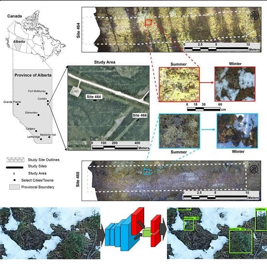
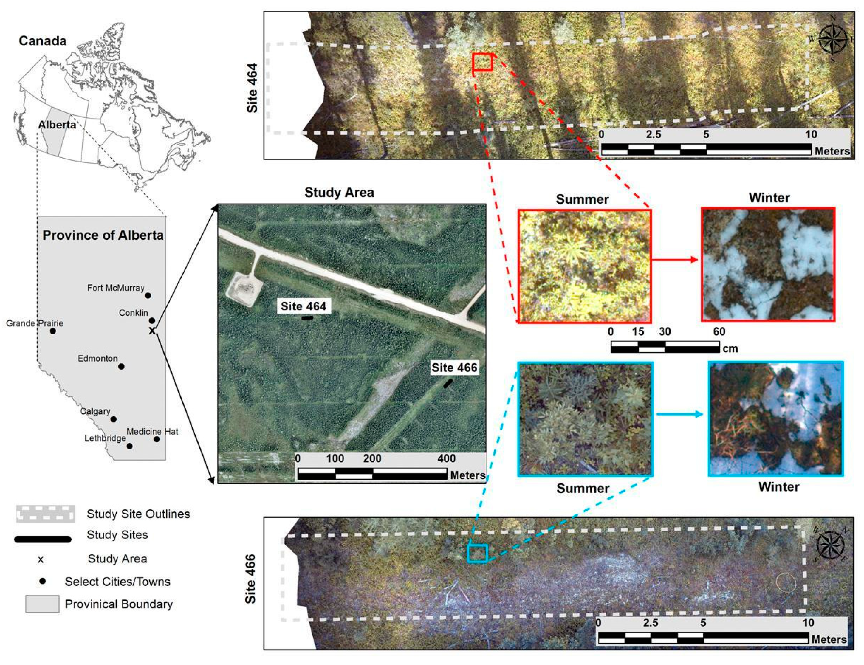
2.1. Study Area
2.2. Image Data
2.3. Image Preprocessing
2.4. Image Annotation
2.5. Automated Seedling Detection Architectures
2.5.1. Object Detection Architectures
2.5.2. Pretrained Feature Maps
2.5.3. Data Augmentation
2.5.4. Seasonal Influence
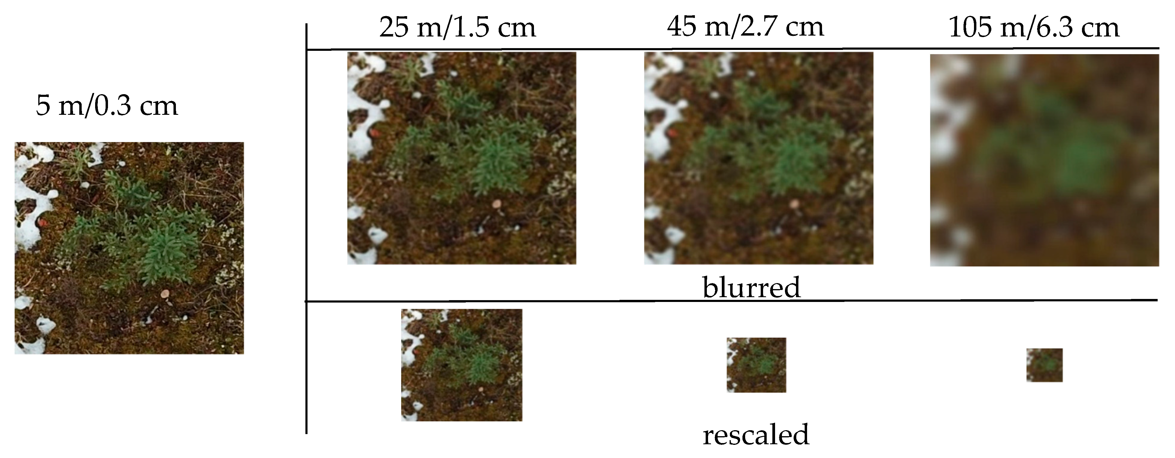
2.5.5. Emulated Flying Altitude and Ground Sampling Distance
2.5.6. Training Set Size
2.5.7. Seedling Size
2.6. Evaluation Metrics for Automated Seedling Detection
3. Results
3.1. Influence of the CNN Used to Generate the Feature Map
3.2. The Effect of Pre-Training
3.3. Data Augmentation
3.4. Seasonal Influence
3.5. Emulated Flying Altitude and Ground Sampling Distance
3.6. Dataset Size
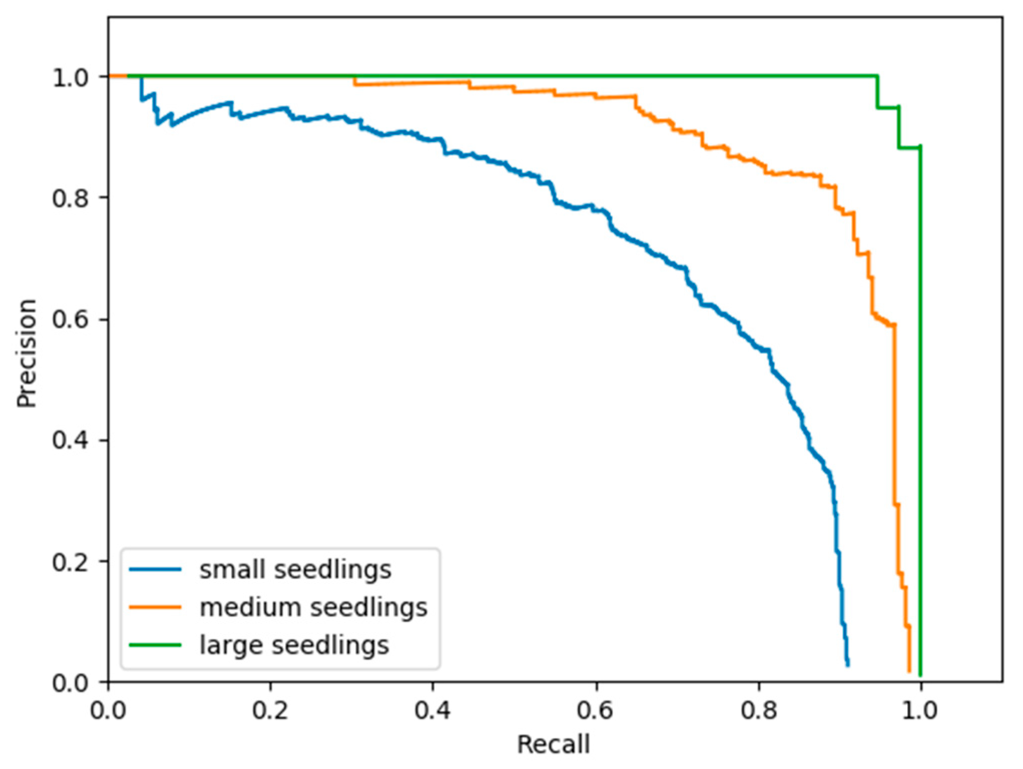
3.7. Seedling Size
4. Discussion
5. Conclusions
Author Contributions
Funding
Acknowledgments
Conflicts of Interest
References
- Goodbody, T.R.; Coops, N.C.; Marshall, P.L.; Tompalski, P.; Crawford, P. Unmanned aerial systems for precision forest inventory purposes: A review and case study. For. Chron. 2017, 93, 71–81. [Google Scholar] [CrossRef] [Green Version]
- Ullman, S. The interpretation of structure from motion. Proc. R. Soc. B 1979, 203, 405–426. [Google Scholar]
- Ciresan, D.; Meier, U.; Schmidhuber, J. Multi-column deep neural networks for image classification. In Proceedings of the 2012 IEEE Conference on Computer Vision and Pattern Recognition, Providence, RI, USA, 16–21 June 2012; pp. 3642–3649. [Google Scholar]
- Dabros, A.; Pyper, M.; Castilla, G. Seismic lines in the boreal and arctic ecosystems of North America: Environmental impacts, challenges, and opportunities. Environ. Rev. 2018, 26, 214–229. [Google Scholar] [CrossRef]
- Hall, R.J.; Aldred, A.H. Forest regeneration appraisal with large-scale aerial photographs. For. Chron. 1992, 68, 142–150. [Google Scholar] [CrossRef] [Green Version]
- Goodbody, T.R.; Coops, N.C.; Hermosilla, T.; Tompalski, P.; Crawford, P. Assessing the status of forest regeneration using digital aerial photogrammetry and unmanned aerial systems. Int. J. Remote Sens. 2017, 39, 5246–5264. [Google Scholar] [CrossRef]
- Puliti, S.; Solberg, S.; Granhus, A. Use of UAV photogrammetric data for estimation of biophysical properties in forest stands under regeneration. Remote Sens. 2019, 11, 233. [Google Scholar] [CrossRef]
- Feduck, C.; McDermid, G.; Castilla, G. Detection of coniferous seedlings in UAV imagery. Forests 2018, 9, 432. [Google Scholar] [CrossRef]
- Ashqar, B.A.; Abu-Nasser, B.S.; Abu-Naser, S.S. Plant Seedlings Classification Using Deep Learning. IJAISR 2019, 3, 7–14. [Google Scholar]
- Ferreira, A.D.S.; Freitas, D.M.; Da Silva, G.G.; Pistori, H.; Folhes, M.T. Weed detection in soybean crops using ConvNets. Comput. Electron. Agric. 2017, 143, 314–324. [Google Scholar] [CrossRef]
- Kamilaris, A.; Prenafeta-Boldú, F.X. Deep learning in agriculture: A survey. Comput. Electron. Agric. 2018, 147, 70–90. [Google Scholar] [CrossRef] [Green Version]
- Scion 2019. Deep Learning Algorithm Can Identify Seedlings. Research Highlight. Available online: http://www.scionresearch.com/about-us/about-scion/corporate-publications/annual-reports/2019-annual-report/research-highlights/deep-learning-algorithm-can-identify-seedlings (accessed on 23 September 2019).
- Zhu, X.X.; Tuia, D.; Mou, L.; Xia, G.S.; Zhang, L.; Xu, F.; Fraundorfer, F. Deep learning in remote sensing: A comprehensive review and list of resources. IEEE Geosci. Remote Sens. Mag. 2017, 5, 8–36. [Google Scholar] [CrossRef]
- Ma, L.; Liu, Y.; Zhang, X.; Ye, Y.; Yin, G.; Johnson, B.A. Deep learning in remote sensing applications: A meta-analysis and review. ISPRS J. Photogramm. Remote Sens. 2019, 152, 166–177. [Google Scholar] [CrossRef]
- Li, W.; Fu, H.; Yu, L.; Cracknell, A. Deep learning based oil palm tree detection and counting for high-resolution remote sensing images. Remote Sens. 2017, 9, 22. [Google Scholar] [CrossRef]
- Branson, S.; Wegner, J.D.; Hall, D.; Lang, N.; Schindler, K.; Perona, P. From Google Maps to a fine-grained catalog of street trees. ISPRS J. Photogramm. Remote Sens. 2018, 135, 13–30. [Google Scholar] [CrossRef] [Green Version]
- Morales, G.; Kemper, G.; Sevillano, G.; Arteaga, D.; Ortega, I.; Telles, J. Automatic Segmentation of Mauritia flexuosa in Unmanned Aerial Vehicle (UAV) Imagery Using Deep Learning. Forests 2018, 9, 736. [Google Scholar] [CrossRef]
- Natural Regions Committee. Natural Regions and Subregions of Alberta; Compiled by Downing, D.J. and Pettapiece, W.W.; Government of Alberta: Edmonton, AB, Canada, 2006. [Google Scholar]
- Environment Canada. Recovery Strategy for the Woodland Caribou (Rangifer Tarandus Caribou), Boreal Population, in Canada; Environment Canada: Ottawa, ON, Canada, 2012. [Google Scholar]
- Dickie, M.M. The Use of Anthropogenic Linear Features by Wolves in Northeastern Alberta. Master’s Thesis, University of Alberta, Edmonton, AB, Canada, 2015. [Google Scholar]
- Government of Alberta. Provincial Restoration and Establishment Framework for Legacy Seismic Lines in Alberta. In Prepared for Alberta Environment and Parks, Land and Environment Planning Branch; Government of Alberta: Edmonton, AB, Canada, 2017; Volume 9, p. 70. [Google Scholar]
- LabelImg, T. Git Code. 2015. Available online: https://github.com/tzutalin/labelImg (accessed on 12 September 2017).
- Ren, S.; He, K.; Girshick, R.; Sun, J. Faster R-CNN: Towards Real-Time Object Detection with Region Proposal Networks. In Proceedings of the NIPS 2015, Montreal, QC, Canada, 7–12 December 2015. [Google Scholar]
- Dai, J.; Li, Y.; He, K.; Sun, J. R-FCN: Object Detection via Region-based Fully Convolutional Networks. In Proceedings of the NIPS 2016, Barcelona, Spain, 5–10 December 2016. [Google Scholar]
- Liu, W.; Anguelov, D.; Erhan, D.; Szegedy, C.; Reed, S.; Fu, C.-Y.; Berg, A.C. SSD: Single Shot MultiBox Detector. In Proceedings of the ECCV 2016, Amsterdam, The Netherlands, 11–14 October 2016; pp. 21–37. [Google Scholar]
- Kingma, D.; Ba, J. Adam: A Method for Stochastic Optimization. In Proceedings of the International Conference on Learning Representations, Banff, AB, Canada, 14–16 April 2014. [Google Scholar]
- Uijlings, J.R.R.; van de Sande, K.E.A.; Gevers, T.; Smeulders, A.W.M. Selective Search for Object Recognition. Int. J. Comput. Vis. 2013, 104, 154–171. [Google Scholar] [CrossRef] [Green Version]
- Christian, S.; Vincent, V.; Sergey, I.; Jonathon, S.; Zbigniew, W. Rethinking the Inception Architecture for Computer Vision. In Proceedings of the 2016 IEEE Conference on Computer Vision and Pattern Recognition 2016, Las Vegas, NV, USA, 27–30 June 2016; pp. 2818–2826. [Google Scholar]
- He, K.; Zhang, X.; Ren, S.; Sun, J. Deep Residual Learning for Image Recognition. In Proceedings of the 2016 IEEE Conference on Computer Vision and Pattern Recognition 2016, Las Vegas, NV, USA, 27–30 June 2016; pp. 770–778. [Google Scholar]
- Christian, S.; Sergey, I.; Vincent, V. Inception-v4, Inception-ResNet and the Impact of Residual Connections on Learning. CoRR 2016, arXiv:1602.07261. [Google Scholar]
- Lin, T.-Y.; Maire, M.; Belongie, S.; Hays, J.; Perona, P.; Ramanan, D.; Dollár, P.; Zitnick, C.L. Microsoft COCO: Common Objects in Context. In Proceedings of the ECCV 2014, Zurich, Switzerland, 6–12 September 2014; pp. 740–755. [Google Scholar]


| Experiment | Train/Test | Site 464 | Site 466 | Total | |||||||
|---|---|---|---|---|---|---|---|---|---|---|---|
| Winter (leaf-off) | Summer (leaf-on) | Winter (leaf-off) | Summer (leaf-on) | ||||||||
| Images | Tiles | Images | Tiles | Images | Tiles | Images | Tiles | Images | Tiles | ||
| Summer | Train | 37 | 387 | 14 | 132 | 51 | 519 | ||||
| Test | 21 | 215 | 21 | 215 | |||||||
| Winter | Train | 59 | 670 | 59 | 670 | ||||||
| Test | 86 | 896 | 86 | 896 | |||||||
| Summer -> Winter | Train | 37 | 387 | 35 | 347 | 72 | 734 | ||||
| Test | 116 | 1177 | 82 | 894 | 198 | 2071 | |||||
| Winter -> Summer | Train | 116 | 1177 | 82 | 894 | 198 | 2071 | ||||
| Test | 37 | 387 | 35 | 347 | 72 | 734 | |||||
| Combination | Train | 32 | 235 | 37 | 387 | 82 | 894 | 35 | 347 | 186 | 1863 |
| Test | 54 | 661 | 54 | 661 | |||||||
| Convolutional Net | Speed (ms) | Parameters | Layers | MS COCO MAP |
|---|---|---|---|---|
| Inception v2 | 58 | 10 M | 42 | 28 |
| ResNet-50 | 89 | 20 M | 50 | 30 |
| ResNet-101 | 106 | 42 M | 101 | 32 |
| Inception ResNet v2 | 620 | 54 M | 467 | 37 |
| Object Detector | Layers | Parameters | COCO MAP | Seedling MAP |
|---|---|---|---|---|
| Inception v2 | 42 | 10 M | 0.28 | 0.66 |
| ResNet-50 | 50 | 20 M | 0.30 | 0.66 |
| ResNet-101 | 101 | 42 M | 0.32 | 0.81 |
| Inception ResNet v2 | 467 | 54 M | 0.72 | 0.71 |
| Object Detector | Without Pre-Training | With Pre-Training |
|---|---|---|
| SSD | 0.65 | 0.58 |
| R-FCN | 0.68 | 0.71 |
| Faster R-CNN | 0.71 | 0.81 |
| Object Detector | No Augmentation | Data Augmentation |
|---|---|---|
| SSD | 0.58 | 0.69 |
| R-FCN | 0.71 | 0.76 |
| Faster R-CNN | 0.81 | 0.80 |
| Object Detector | Summer | Winter | Both |
|---|---|---|---|
| SSD | 0.45 | 0.41 | 0.65 |
| R-FCN | 0.69 | 0.59 | 0.71 |
| Faster R-CNN | 0.71 | 0.65 | 0.81 |
| Object Detector | 5 m/0.3 cm | 25 m/1.5 cm | 45 m/2.7 cm | 105 m/6.3 cm |
|---|---|---|---|---|
| SSD | 0.58 | 0.56 | 0.50 | 0.45 |
| R-FCN | 0.71 | 0.66 | 0.67 | 0.57 |
| Faster R-CNN | 0.81 | 0.75 | 0.72 | 0.66 |
| Object Detector | 5 m/0.3 cm | 25 m/1.5 cm | 45 m/2.7 cm | 105 m/6.3 cm |
|---|---|---|---|---|
| SSD | 0.58 | 0.56 | 0.17 | 0.00 |
| R-FCN | 0.71 | 0.72 | 0.16 | 0.00 |
| Faster R-CNN | 0.81 | 0.78 | 0.22 | 0.02 |
| Object Detector | Pre-Trained | 200 | 500 | 1000 | 2000 | 3940 |
|---|---|---|---|---|---|---|
| SSD | () | 0.15 | 0.24 | 0.36 | 0.48 | 0.65 |
| R-FCN | () | 0.39 | 0.49 | 0.58 | 0.61 | 0.68 |
| Faster R-CNN | () | 0.52 | 0.59 | 0.62 | 0.65 | 0.71 |
| SSD | (×) | 0.16 (+1%) | 0.30 (+6%) | 0.39 (+3%) | 0.51 (+3%) | 0.58 (–7%) |
| R-FCN | (×) | 0.66 (+27%) | 0.67 (+18%) | 0.69 (+11%) | 0.73 (+12%) | 0.71 (+3%) |
| Faster R-CNN | (×) | 0.68 (+14%) | 0.70 (+11%) | 0.75 (+13%) | 0.76 (+12%) | 0.81 (+10%) |
| Object Detector | Small | Medium | Large | All |
|---|---|---|---|---|
| SSD | 0.43 | 0.79 | 0.99 | 0.58 |
| SSD (aug) | 0.55 | 0.84 | 0.97 | 0.65 |
| R-FCN | 0.48 | 0.85 | 0.99 | 0.71 |
| Faster R-CNN | 0.72 | 0.91 | 1.00 | 0.81 |
© 2019 by the authors. Licensee MDPI, Basel, Switzerland. This article is an open access article distributed under the terms and conditions of the Creative Commons Attribution (CC BY) license (http://creativecommons.org/licenses/by/4.0/).
Share and Cite
Fromm, M.; Schubert, M.; Castilla, G.; Linke, J.; McDermid, G. Automated Detection of Conifer Seedlings in Drone Imagery Using Convolutional Neural Networks. Remote Sens. 2019, 11, 2585. https://0-doi-org.brum.beds.ac.uk/10.3390/rs11212585
Fromm M, Schubert M, Castilla G, Linke J, McDermid G. Automated Detection of Conifer Seedlings in Drone Imagery Using Convolutional Neural Networks. Remote Sensing. 2019; 11(21):2585. https://0-doi-org.brum.beds.ac.uk/10.3390/rs11212585
Chicago/Turabian StyleFromm, Michael, Matthias Schubert, Guillermo Castilla, Julia Linke, and Greg McDermid. 2019. "Automated Detection of Conifer Seedlings in Drone Imagery Using Convolutional Neural Networks" Remote Sensing 11, no. 21: 2585. https://0-doi-org.brum.beds.ac.uk/10.3390/rs11212585