Modeling Population Density Using a New Index Derived from Multi-Sensor Image Data


Institute of Remote Sensing and Geographic Information System, Peking University, 5 Summer Palace Road, Beijing 100871, China
*
Author to whom correspondence should be addressed.
Remote Sens. 2019, 11(22), 2620; https://0-doi-org.brum.beds.ac.uk/10.3390/rs11222620
Submission received: 30 September 2019
/
Revised: 6 November 2019
/
Accepted: 7 November 2019
/
Published: 8 November 2019
(This article belongs to the Special Issue Global Geospatial Information and Hazards Management for Smart Environments)
Abstract
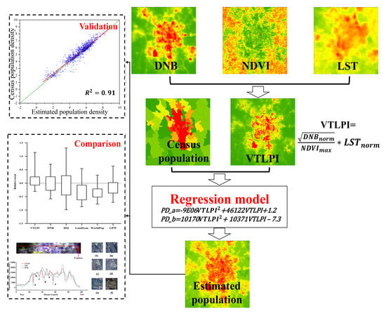
:The detailed information about the spatial distribution of the population is crucial for analyzing economic growth, environmental change, and natural disaster damage. Using the nighttime light (NTL) imagery for population estimation has been a topic of interest in recent decades. However, the effectiveness of NTL data in population estimation has been impeded by some limitations such as the blooming effect and underestimation in rural regions. To overcome these limitations, we combine the NPP-VIIRS day/night band (DNB) data with normalized difference vegetation index (NDVI) and land surface temperature (LST) data derived from the moderate resolution imaging spectroradiometer (MODIS) onboard the Terra satellite, to create a new vegetation temperature light population index (VTLPI). A statistical model is developed to predict 250m grid-level population density based on the proposed VTLPI and the least square regression approach. After that, a case study is implemented using the data of Sichuan Province, China in 2015, and the results indicates that the VTLPI-estimated population density outperformed the results from other two methods based on nighttime light imagery or human settlement index, and the three publicized population products, LandScan, WorldPop, and GPW. When using the census data as reference, the mean relative error and median absolute relative error on a township level are 0.29 and 0.12, respectively, and the root-mean-square error is 212 persons/km2. The results show that our VTLPI-based model can achieve a better estimation of population density in rural areas and urban suburbs and characterize more spatial variations at 250m grid level both in both urban and rural areas. The resultant population density offers better population exposure data for assessing natural disaster risk and loss as well as other related applications.
1. Introduction
Population is one of the most explicit indicators for characterizing human activities, and thus, population data are extensively used in the fields of ecological and environmental modeling, urban planning, public health assessment, and resource development [1,2,3,4]. Accurate and detailed information of the spatial patterns of population density is an important part of disaster risk management [1,5], and spatial superposition analysis of the strength of natural hazard factors such as seismic intensity and the elements at risk such as population exposure is a key step in risk assessment of various natural disasters [5]. Hence, it is necessary for emergency rescue and disaster relief to access quality data of population exposure in disaster situations.
Census data are currently the most available population data usually being captured based on administrative units. Despite their authoritativeness, some limitations have hampered the usefulness of population census data. First, the census method is time-consuming and extremely expensive, and consequently population census work can only be conducted in every specific years [6]. For instance, the Chinese government conducts countrywide population census regularly every 10 years, and 1% population sampling survey is usually conducted between the two census times. The latest countrywide census work and sampling survey in China were finished in 2010 and 2015, respectively. Second, because the census data are usually collected on administrative units, they cannot provide spatially explicit details, which are necessary to describe the spatial distribution of human population in the administrative units [7,8,9]. Third, it often happens that the study area for a specific study is inconsistent with the census boundary and consequently spatial mismatching problems have arisen when the census data are adopted in these applications [10]. The spatial mismatching presents a persistent problem in geography, planning, hazard analysis and other fields [11]. Finally, due to the change of unit boundaries among different census years, the temporal inconsistency problem may exist, which impedes demographic temporal comparison and analysis [12,13,14].
With the development of new technologies such as geographic information systems (GIS) and remote sensing, alternative methods have been developed to disaggregate the census data [8,15]. Among them, areal weighting and dasymetric methods are the most widely used ones. As for the areal weighting method, the population within source areas is spatially apportioned into the target areas based on how much of each source area falls within each target area [16]. This method does not use any other geographic data and assumes that the population density is distributed evenly over the administrative units [17]. The gridded population data of the world (GPW, http://sedac.ciesin.columbia.edu/data/collection/gpw-v4) released by the Center for International Earth Science Information Network is one of the most widely used population datasets created by the areal weighting approach [16]. The main advantage of this method is the maintenance of the fidelity of the input data and can be easily updated [17]. However, its performance is dependent on the assumption of homogeneous population density, and in fact, the human beings are usually distributed in a non-uniform or clumped way [18]. Thus, although the areal weighting method is simple and requires very few variables, it is hard to reflect the details at a grid cell location and the accuracy of downscaling population products needs to be improved based on some other information.
The dasymetric mapping method was developed to improve the areal weighting method [19]. Census data are apportioned into each grid cell based on the weights derived from auxiliary data, and land cover data are the most widely used ancillary data for the implementation of the dasymetric mapping [8,20,21]. The global population dataset, LandScan (https://landscan.ornl.gov/), was created using a dasymetric mapping approach by the Oak Ridge National Laboratory (ORNL), USA. Different from the GPW product, a residential population dataset, the LandScan dataset represents an ambient population product, which means average population distribution over a 24-h time period [18]. Ambient population density is a temporally averaged measure of population density that incorporates human mobility, which takes into account where people work, relax, commute, etc. Hence, it can be a more useful representation for many applications such as hazard loss assessment and crime analysis [22]. In addition, the WorldPop dataset (www.worldpop.org/) used random forest model to disaggregate population from census data, providing a finer population grid at 100 × 100 m resolution [18,19]. The dasymetric mapping method can combine multi-source data for population estimation, but some auxiliary data may not be available at large ranges, and the determination of the weight for each variable is complicated and time-consuming [5]. In addition, both the dasymetric mapping and area weighting methods might be affected by the modifiable areal unit problem (MAUP) [23,24], which arises as a result of statistical analysis by being performed on different combinations of aggregated data with scale effects and different subzones [2,3].
To overcome the drawbacks of the abovementioned methods and improve the accuracy of population data products, some new remotely sensed data were utilized to create more effective and robust spatial statistical models to characterize population distribution over an area better [5,25,26]. Land cover data were primarily used in the modeling of the spatial distribution of population in early years [6,8,15,27], but the resultant population density is limited in accuracy due to the insufficient characterization of human activities in the land cover data. One improvement is the use of nighttime light (NTL) imagery in the modeling of population density over a large area [5,10,20,24,26,28,29,30]. For instance, NTL data from Defense Meteorological Satellite Program’s Operational Line-Scan System (DMSP-OLS), sensors have been used extensively as a proxy of human activities, but the use is hampered by several limitations, including insufficient dynamic range, blooming effect, and saturation effect [31,32,33]. The National Polar-Orbiting Partnership/Visible Infrared Imaging Radiometer Suit (NPP/VIIRS) is a new generation sensor and the 16-bit NPP/VIIRS DNB data have great improvement in spatial and radiometric resolution [34]. Thus, the NPP/VIIRS DNB can better identify weak light sources and is more suitable for estimating socioeconomic [35,36] and population distribution [26,37]. However, it is worth noting that the use of NTL data in the modeling of population distribution may lead to underestimation in rural areas, especially in the rural villages and small towns of undeveloped countries, and thus they were mostly adopted to estimate the population in urban areas [7,30,38,39]. Besides, using NTL data alone may lead to unreasonable estimation in some specific areas, for example, some researchers reported the overestimation in commercial zones and underestimation in residential areas affected by the lamp types and lamp density [40], and the overestimation in urban green space affected by the blooming effect in the NTL data.
A recent trend is to incorporate NTL data together with some other data sources, to improve the estimation of population density further [7,29]. Besides the land cover data, vegetation index (VI) was also used in the estimation of population distribution, which can reduce down errors in the estimation of human settlements or built-up areas from NTL data [41,42]. For example, the human settlement index (HSI) [41] that incorporates DNB with VI was used to estimate the population of Zhejiang Province, China [5]. Speaking generally, integration of NTL, VI and land cover data can reveal more spatial variations of population distribution, but we still need to examine some drawbacks and problems deliberately. First, the ability of current methods is still insufficient to estimate the population in some small residential areas, particularly in rural or suburban areas because of very low nighttime light values in these areas, which made it hard to detect by NTL satellite sensors. Second, the human habitats in these areas are relatively small and often fragmented in rural areas, and difference of the NDVI or land cover types between the human habitats and the surrounding bare soil lands is relatively small. Therefore, using VI or land cover data to estimate the population distribution in these areas may cause large deviations. Third, radiance variations within rural and suburban areas are suppressed [43], and consequently, if only using the NTL data for population estimation, there may be overestimation in urban areas while underestimation in suburbs and countryside villages. Finally, the NTL and VI are very susceptible to other factors such as economic development levels, leading to some unreasonable estimation of population distribution [44].
This study intends to incorporate NPP-VIIRS DNB, MODIS VI, and LST, and land cover data into the modeling of population density over a large area to overcome the aforementioned disadvantages and drawbacks in the use of NTL data for the estimation of population density. A case study in Sichuan Province, China with our proposed model is to be implemented and presented in Section 3 to demonstrate the usefulness of our model, and finally discussion and conclusion are described respectively in Section 4 and Section 5.
2. Data and Method
2.1. Data Collection and Preprocessing
The remotely sensed data used in this study include NPP/VIIRS DNB, MODIS NDVI, and LST, and 30m FROM-GLC (Finer Resolution Observation and Monitoring of Global Land Cover) data. The Shuttle Radar Topography Mission (SRTM) digital elevation model (DEM) data covering the study area and related census data are also collected. All the remote sensing image data were downloaded and preprocessed using the Google Earth Engine (GEE). GEE is a cloud-based geospatial processing platform supported by Google’s cloud infrastructure that provides free PB-level global scale geoscience data [45,46]. The computation in GEE is based on automated parallel processing of Google infrastructure, which significantly improves the efficiency of the data processing [47,48].
The NPP-VIIRS DNB composite data with a spatial resolution of 15 arc-seconds (about 500 m) were produced by the National Geophysical Data Center, NOAA, USA (https://www.ngdc.noaa.gov/eog/viirs/download_dnb_composites.html) [40]. As a preliminary product, they contain light intensity from human activity areas, fires, gas flares, volcanoes, and auroras [44,49]. Some pixels with negative values in the NPP-VIIRS data may be caused by the background noise of the data [29], and there are some abnormal big pixel values in the original NPP-VIIRS data, which may be associated with the light reflected by high reflectance surfaces (e.g., snow-capped mountains). Therefore, the original NPP-VIIRS data have to be corrected as follows. First, the VIIRS-DNB images for 12 months of the year were averaged so that each pixel in the image represents the annual average brightness to address the issue of abrupt brightness [50]. Second, the maximum light intensity value of the most developed cities was selected as the maximum value for all the pixels in the study area, and those values larger than it were replaced by the maximum value [51]. Furthermore, the pixels with negative values were replaced with zero value [29]. However, small light values in water and snow areas still existed in the images. Since these values are irrelevant to human activities and maybe resulted from the reflected moonlight at night by water bodies, the water and snow mask created from the FROM-GLC data were applied to remove these noises by setting their pixel values as zero. After the preprocessing abovementioned, the VIIRS-DNB data were re-projected into Albers conical equal-area (ACEA) projection and resampled to 250 m images using the bilinear interpolation algorithm.
The 16-days Terra MODIS NDVI products (MOD13Q1) at a spatial resolution of 250 m were created from atmospherically corrected bidirectional surface reflectance and masked for water, cloud, heavy aerosol, and cloud shadows [52,53]. In order to eliminate the impact of bare soil, cloud contamination and solar elevation angles, maximum value composition (MVC) method was applied to create an annual maximal NDVI image, and they were also projected into the ACEA projection using the nearest-neighbor algorithm [33]. The MODIS LST data are the MOD11A2 that provides an average 8-day land surface temperature in a 1200 × 1200 m grid [33]. Each pixel value in MOD11A2 is a simple average of all the corresponding MOD11A1 LST pixels collected within that 8-day period. The annual mean composition was applied to create a mean LST image of a year, which enables to simulate the ground surface temperature and reduce the sensitivity of the LST to seasonal variations [54]. If a certain pixel has a value on several dates, the average is applied to them, and if it has a value only at one date, the value of that date is used as the synthesized value of the pixel in question. This processing can also fill in those missing values and eliminate outliers effectively. Finally, the mean LST imagery was then re-projected into the ACEA projection using the nearest-neighbor algorithm and resampled to a 250-m resolution. It should be mentioned that nearest-neighbor algorithm was selected to resample NDVI and LST images for the reason that LST and NDVI have explicit physical meanings, and the values are very sensitive to changes over land cover types. Therefore, we use the nearest-neighbor algorithm to try to keep the original values after resampling the NDVI and LST images.
The SRTM/DEM v3 product (SRTM Plus) provided by NASA JPL is at a resolution of one arc-second, approximately 30 m [55]. The DEM data were re-projected into the ACEA projection and resampled to 250 m using the bilinear interpolation algorithm, which can maintain smoother interpolation in the resampling.
In addition, Land cover data, the 30 m FROM-GLC 2015 were used as reference data with which to validate the performance of the vegetation temperature light population index (VTLPI). The classification system includes 10 types of land covers, including cropland, forest, grassland, wetland, water, tundra, impervious surface, bare land, and cloud [56]. The FROM-GLC data covering the study area were clipped and re-projected to the same projection system. The impervious surface class of FROM-GLC data was used as the urban class in this study, and the percentages within 250-m urban grid cells were calculated for each pixel and the urban fraction image was formed with the pixel values ranging from 0 to 1.
2.2. Vegetation Temperature Light Population Index
Since different remotely sensed data have their own advantages and can offer different information for characterizing population distribution, the combination of multi-source data could provide a more accurate estimation of population density than individual sensor data [41]. Therefore, we will examine the combination of different remote sensing data and create a new and effective index for the estimation of population density.
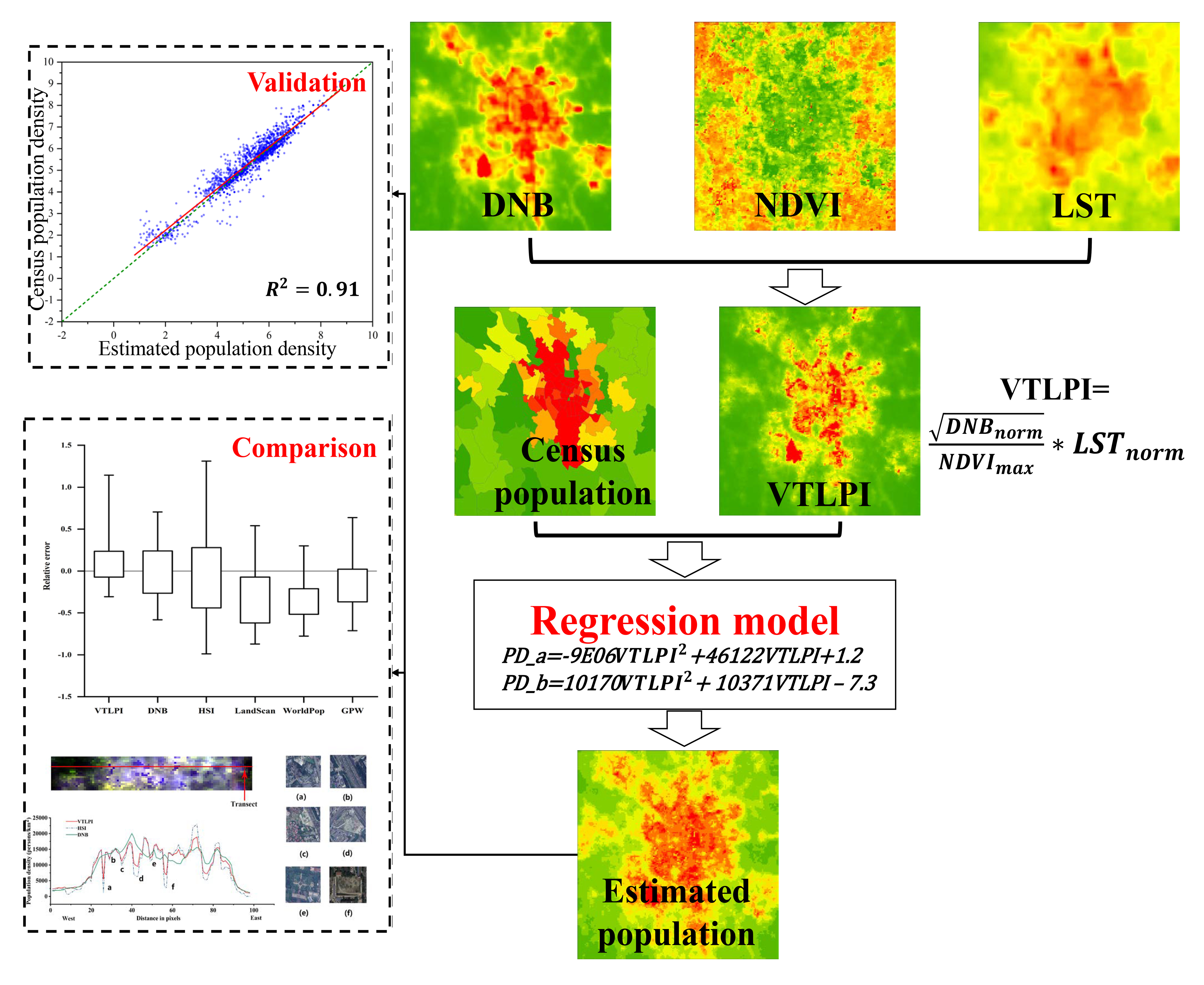
The NTL images are one of the most important data to reveal population activity and our proposed method uses NPP VIIRS DNB data for population estimation. However, as we already mentioned in the section of the introduction, because of the imbalance in radiance distribution of NPP VIIRS DNB data, the population density may be overestimated in urban areas and underestimated in suburbs and rural villages. To this end, we use the square root transformation to smooth this effect [43,44]. As can be seen in Figure 1, the radiance jump within the downtowns in the study area has been suppressed and the radiance variance outside the city has been enhanced after the square root transformation.
For example, before the transformation, the maximum light value at the longitude of 104.04°E inside the city is nearly 60 times the light value at the longitude of 103.62°E in the suburbs. However, after the transformation, the difference of the transformed NTL values between these two locations is only about 14 times. If the original NTL data are directly used to estimate population density, it tends to distribute the population excessively into the urban area. Therefore, using the transformed NTL data to estimate the population density will alleviate the overestimating problem in the urban area. As a result, the NPP/VIIRS DNB radiance after the transformation has distinct variations and the human activities with small NTL values can be detected better by using the transformed NTL images especially in the suburbs and rural areas. In addition, some areas such as airports and tall buildings have extremely high DNB values [57], which may lead to the overestimation of the population in these areas, and the square root transformation can also remove the impact of this phenomenon [44].
Although NTL is a good indicator for human activity, demographic information reflected by the NTL data alone is insufficient. VI can reflect human activities and quantify land cover properties [33], and usually negatively correlated with urban impervious surfaces [58]. A high fraction of settlements has larger digital number (DN) values in NTL imagery and smaller DN values in NDVI imagery. Hence, the combination of VI and NTL has been used together for extracting the impervious layers and urban ranges [41]. Some studies combine NTL with land cover data and VI data for urban studies and population estimates.
As an important environmental variable, LST is also closely related to different land covers and is therefore widely used in land use and land cover classification [59] as well as urban extraction [33,60,61]. However, there are still few studies using LST to enhance the estimation of population density. Thus, we intend to explore the incorporation of LST information into the new index formation to estimate population density mainly for the following reasons. Previous research has proven that there is a significant temperature gradient between urban and rural areas [62]. Therefore, LST can reflect urban-rural differences. At the same time, the correlation between LST and impervious surface area (ISA) is significant [63], and the proportion of ISA can show the mixed land use types in urban areas. Therefore, LST can reflect the spatial distribution of the population. In addition, human habitats in rural areas often have similar NDVI values with surrounding rural areas, but due to differences in heat exchange, LST in urban environment varies widely. Therefore, the LST information can enhance the distinguishing of the impervious layer both in urban and rural areas, and thus can reflect the difference in population distribution between urban and rural areas. In addition, the relationship between LST and VI is closely related to urban land use types and can be used to assist in land cover mapping and land use change analysis. This relationship is represented by the LST–NDVI feature space. Since different land covers are situated in different locations in the LST-NDVI feature space [64,65,66,67], the ratio between the LST and NDVI can increase the ability to identify features [66,68,69] and has proven to be an effective aggregate measure for large-scale land cover classification. Therefore, the difference of population distribution in different land cover types can be detected and the accuracy of the estimation of population density is expected to be improved by using the ratio between the LST and NDVI.
Furthermore, although the blooming effect of VIIRS data has significantly been removed [70], some green lands in the central urban areas may still be affected by the surrounding built-up areas that have much higher NTL values, resulting in the overestimation of the population in the green land. Such problems can be resolved to some extent by the ratio of LST and NDVI. For example, the urban built-up area has a higher LST but lower NDVI, while the vegetation area—such as urban green space, farmland, forestland, etc.—is the opposite. In addition, some bare soil areas have lower NDVI values, but generally also have lower LST values than built-up areas. The usefulness of LST in the modeling of population can be illustrated in Figure 2. It is seen that the NDVI values decreased around the locations of A, B, and C, where are located the snow-covered areas or bare hilly areas with smaller NDVI values. If only using VI and NTL to estimate the population density, it may lead to overestimation according to the decrease of the NDVI values in these three areas. Considering the temperatures in these areas are also relatively low, the overestimation can be reduced down to a large extent with the introduction of LST information into the modeling. Thus, we developed a new index termed vegetation temperature light population index (VTLPI) by combining the ratio between the LST and NDVI with VIIRS/DNB data in our study.
where DNBnorm denotes the normalized DNB. NDVImax and LSTnorm are the maximum composite NDVI and normalized LST, respectively. It should be mentioned that the use of NDVI is not a general requirement and other vegetation indices (e.g., enhanced vegetation index, EVI) can be used in the formation of VTLPI. To keep all data sources in the same range between 0 and 1, the LST image is normalized with Equation (2).
where is the normalized with range [0,1], and is the original . , is the minimum LST and maximum LST, respectively. Similarly, the DNB image is also normalized using Equation (3).
where is the normalized DNB with range [0,1], and is the original . , is the minimum and maximum DNB, respectively.
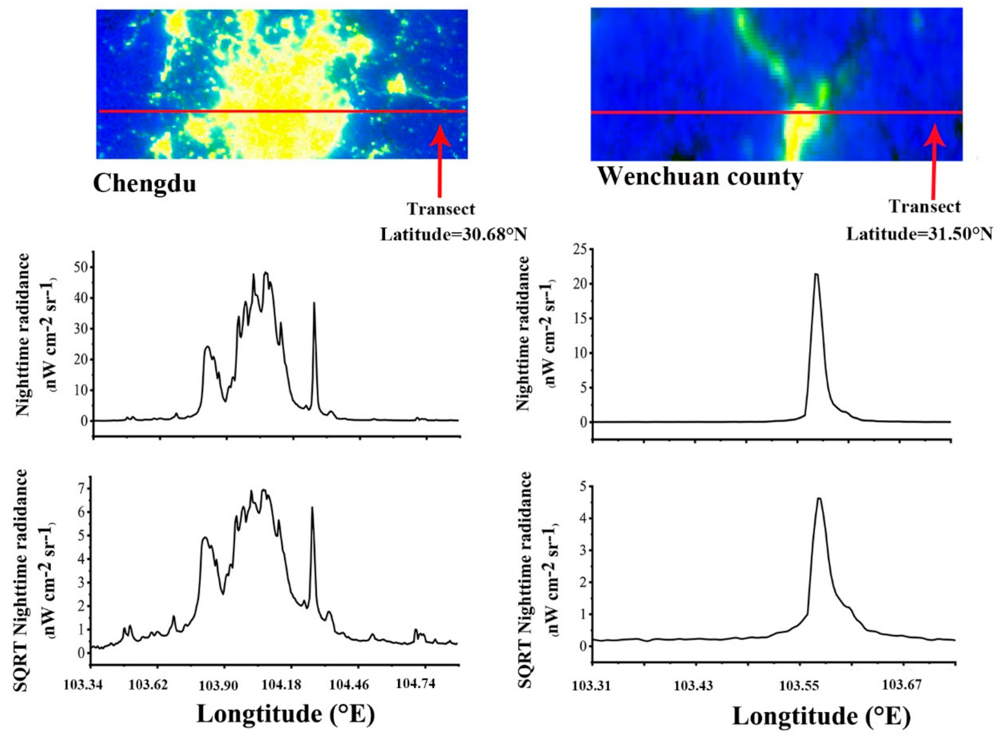
To demonstrate the usefulness of the proposed VTLPI index in reflecting human activities, a transect profile from the west to east on the false color composite image (R=DNB, G=Urban percentage and B=VTLPI) of the Chengdu City was generated (Figure 3). It can be seen in Figure 3 that the proposed VTLPI index is more sensitive to changes in human activities and urban components than the DNB, and the urban percentage is well correlated with the VTLPI. Therefore, the VTLPI index can reflect the spatial distribution characteristics of the population in different regions and increase the details of population changes, and as a result, it can offer a better modeling of population distribution.
2.3. Elevation Correction of VTLPI
Due to the heterogeneity of urbanization among different regions, the models for population estimation in different sub-regions should be adjusted and optimized [40]. The incorporation of VI might introduce the VTLPI values over unlit areas at high elevation or with densely vegetated areas that are general not habitable. Consequently, the VTLPI may result in the overestimation of population density in high altitude areas. Therefore, considering the correlation between population distribution and elevation, a zonal modeling strategy was used to reduce the geographic difference of land covers and customize model parameters for local regions [8]. The elevation correction method proposed by Yang et al. [5] is modified and adapted to enhance the accuracy of population estimation in mountainous areas. Therefore, before the proposed index VTLPI is used to model the spatial distribution of population, we apply the elevation correction to the index VTLPI. Assuming that there is a threshold elevation value D, it can be used to classify all the census units in the study area into region A (where average elevation values are greater than D) and region B (where average elevation values are smaller than D).
According to Yang et al. [5], the D value was subjectively decided based on a visual check to the scatterplot between the population density and averaged DEM values of the counties in question. To derive this parameter better, we proposed a quantitative partitioning method in our study, finding an optimal D value to achieve maximum correlative coefficients in both regions A and B. Starting with a small value of D, then increase it gradually with a certain step. For each D value, the administrative units for population census are grouped into regions A (≥D) and region B (<D) based on the average elevation of the census unit (e.g., county). The correlation coefficient between the elevation and natural log-transformed population density in areas A and B is calculated, respectively, and , and then is obtained by summing the absolute values of these two coefficients. The D value that achieves maximum is adopted finally to perform the elevation correction. After that, the exponential regression model can be created between population density and mean elevation of each census unit in Region A (e.g., county) as Equation (4).
where α is the constant coefficient of the regression equation, C is the coefficient for elevation correction, H is averaged elevation of each census unit in Region A, and POP is averaged population of each census unit. Consequently, the VTLPI can be modified to remove the elevation effect in region A using Equation (5).
where VTLPIcorr is the elevation corrected VTLPI, C is the coefficient for elevation correction, and H is averaged elevation of each census unit in Region A.
2.4. Modeling of Population Density based on VTLPI
Based on the proposed VTLPI index, two least square regression (LSR) models for estimating county-level population density at region A and region B are created to characterize the relationship quantitatively between the population density and the average VTLPI of each census unit (e.g., county).
After masking the water bodies and snow areas, the average VTLPI values over a county is calculated from the elevation corrected VTLPI images.
where xi is the average VTLPI of i-th county, DNij is the VTLPI of pixel j in the county i, and Ni is the total number of the pixels at county i.
It has been proved that LSR in population modeling can achieve better stability, robustness, and predictive capacity at both local and regional levels than other models such as geographically weighted regression (GWR) models [30]. The cross-validation strategy is adopted to select the most appropriate regression equations to guarantee them to work efficiently and prevent overfitting. For every region, the census data are randomly divided into two parts, 70% for training and 30% for testing, and the root-mean-square error (RMSE) calculated from the testing data set is used as a criterion to decide on the selection of an optimal model. The sample dataset is scrambled multiple times, and the training set as well as the testing set is reselected, and the RMSE is re-calculated every time. Finally, the models with the smallest average RMSE are chosen to predict population density in the study area.
The selected regression models are used to predict the spatial distribution of population density in the region A and region B. In the county level, the modeled total population may not exactly equal to the corresponding census values of the same counties, especially when the regression models are nonlinear. Hence, the estimated total population should be further calibrated using the census data to obtain the population density value for each grid of each county [10,25]
where and are the population density of grid j in county i before and after calibration, respectively. is the census population in county i and is the total estimated population of county i before calibration.
2.5. Validation
Accuracy assessment is a critical step for population estimation. Besides and RMSE, the mean relative error (MRE) is a good indicator to quantify the performance of the model [5,59,71] and calculated using Equation (8).
The RE is the ratio of the difference between the estimated and census population to the census population at county i, and n is the total number of counties in the study area. Median absolute relative error (MdRE) is also used in this study because the MRE is sensitive to extreme values. To evaluate the proposed index VTLPI, the two state-of-the-art regression models for population estimation, DNB-based [26,38,72,73] and HSI-based [5,20] as well as other publicized population products are chosen for comparison, and the township-level sampling surveyed data are used as reference to validate the modeling results.
3. Results
3.1. Implementation of the Proposed Model
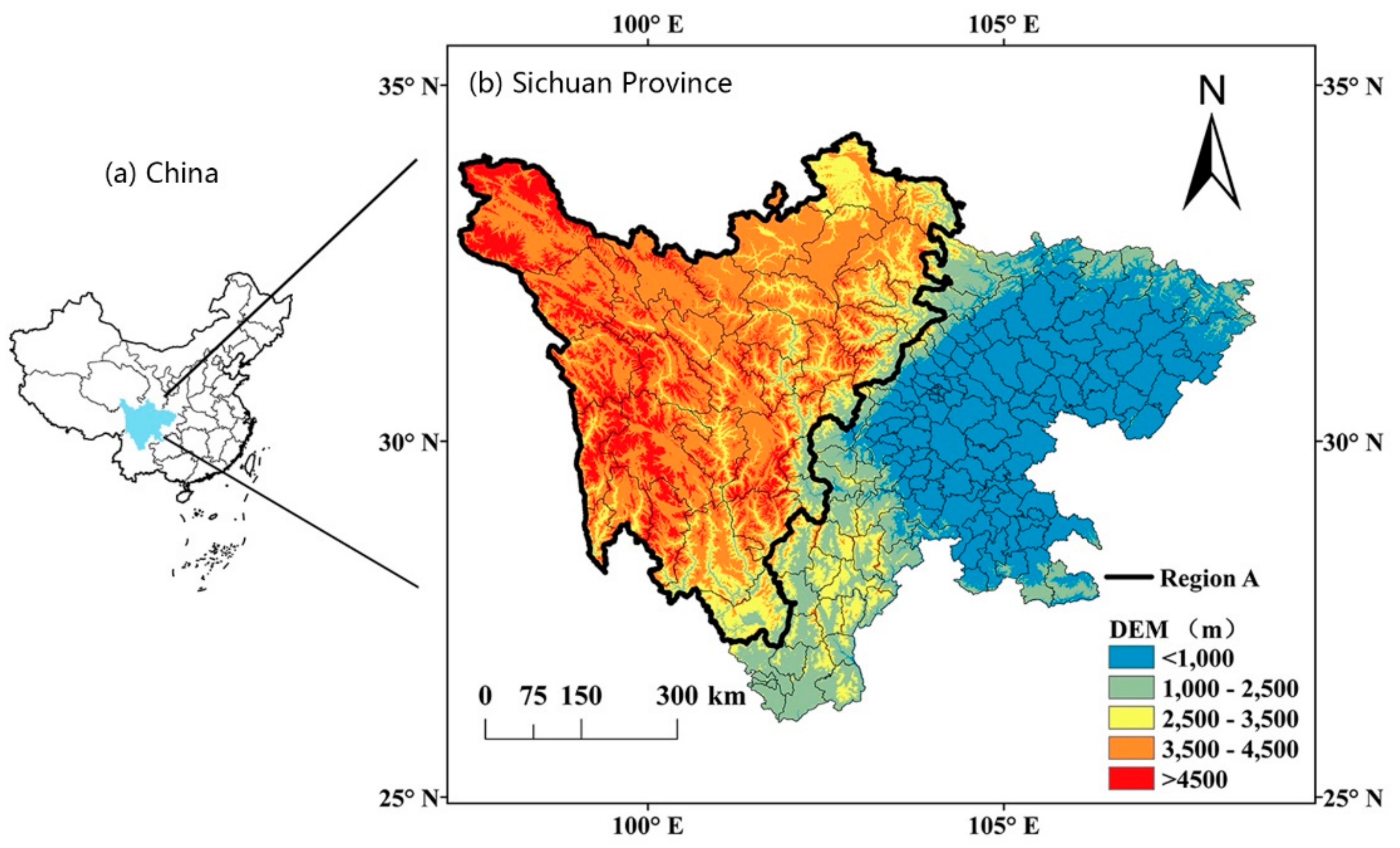
To demonstrate the effectiveness of our proposed approach, a case study in Sichuan Province of China, where people are in high risk of earthquakes and the frightened Wenchuan earthquake took place in the west of the Chengdu City on May 12, 2008, has been implemented and presented in this section using the related data of the year 2015. Sichuan province consists of 181 counties in total and the county-level sampling surveyed population data in these counties were used as initial input in our study. The population sampling survey work was conducted in 2015 covering a population of about 14 million, and the smallest spatial unit for population data gathering is township. It should be mentioned that the sampling census data used in this study were the resident population instead of the household registration population. According to the definition, the resident population refers to the population who live at home all the time or at home for more than six months, including immigrants.
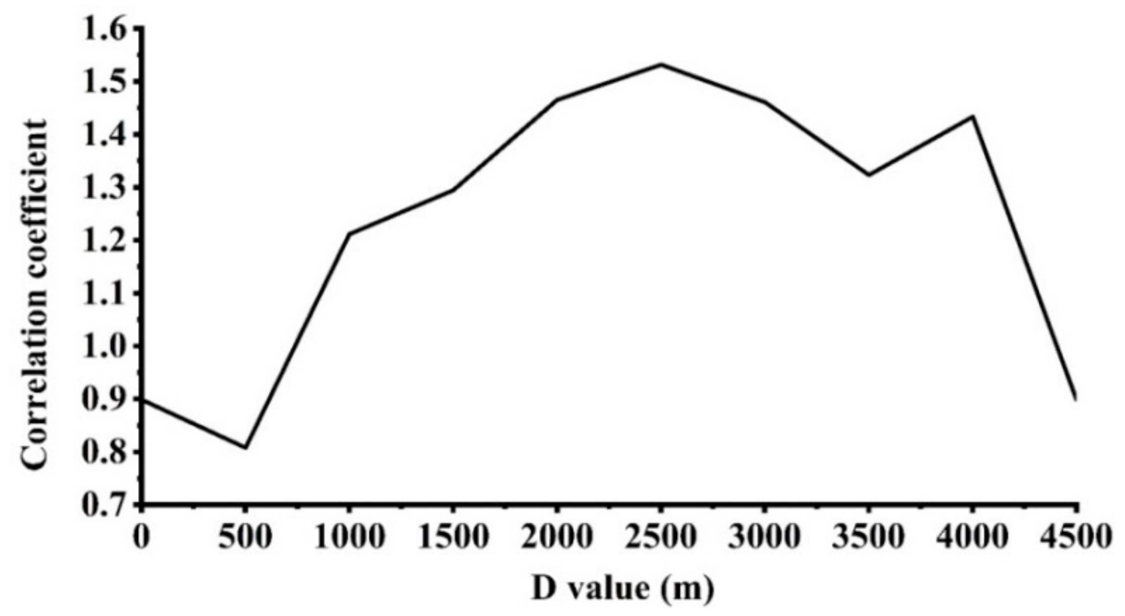
The terrain of Sichuan Province is very complex, and mountains, plateaus, and hills account for 97.46% of the total land area of the province. In the elevation correction, we set an initial value of 0 m for D and increase it by a step of 500 m, to calculate the correlation coefficients of region A and region B as well as at each D value (Figure A1). It can be seen in Figure A1 that when D equals to about 2500 m, reaches the maximum, so we finally selected 2500 m for the parameter D. The counties with an average elevation above 2500 m were categorized into region A, including 37 counties, and the rest of 146 counties make up of region B (Figure 4).
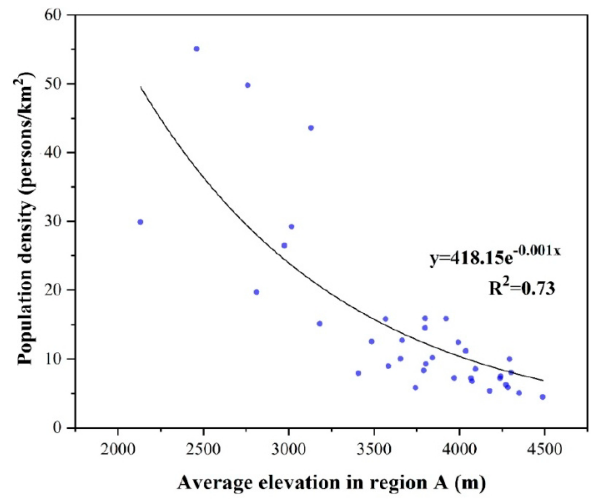
Figure 5 showed the relationship between the population density and mean elevation at the county level in Region A. Same as the finding in reference [5], the relationship can be described by the e-based exponential function. Based on the regression analysis, it was observed that the population density and elevation were highly correlated with of 0.73. C was a coefficient decided by the relationship between the population density and averaged elevation of each county in region A, and the value -0.001 is assigned to C based on the statistical analysis (Figure 5) and used to calibrate the VTLPI in region A using Equation (5).
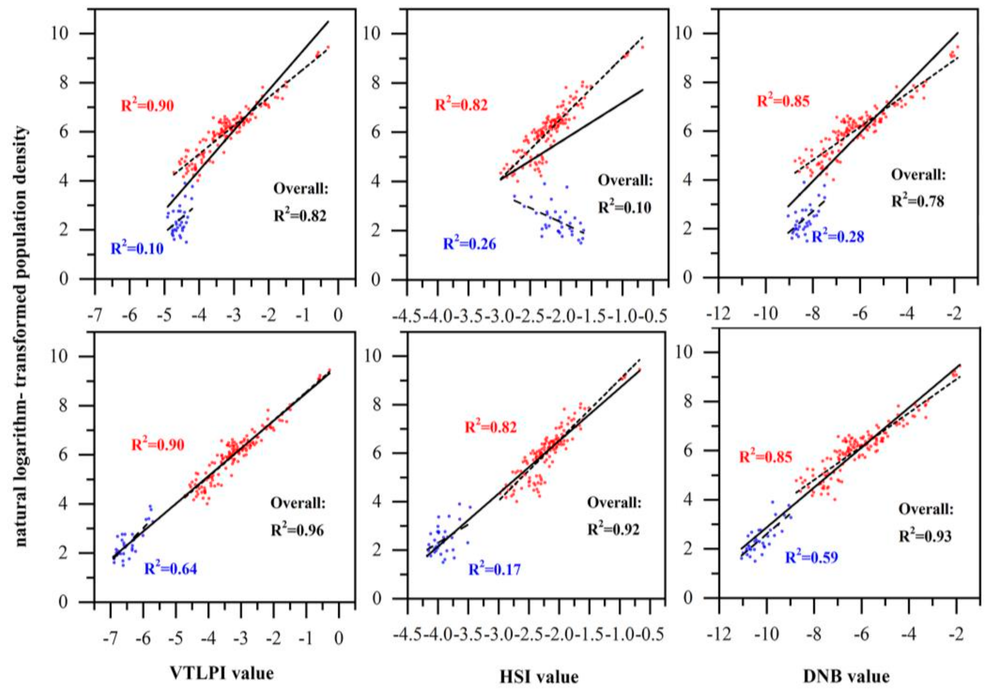
The correlation between VTLPI, HSI, and VIIRS/DNB and natural logarithm-transformed population density at the county-level in Sichuan Province is illustrated in Figure 6 in which the blue dots belong to region A and red dots belong to Region B. It can be seen that the correlation between the population density and the three indices can be significantly improved after the elevation correction with the of VTLPI-based regression model increasing from 0.10 to 0.64.
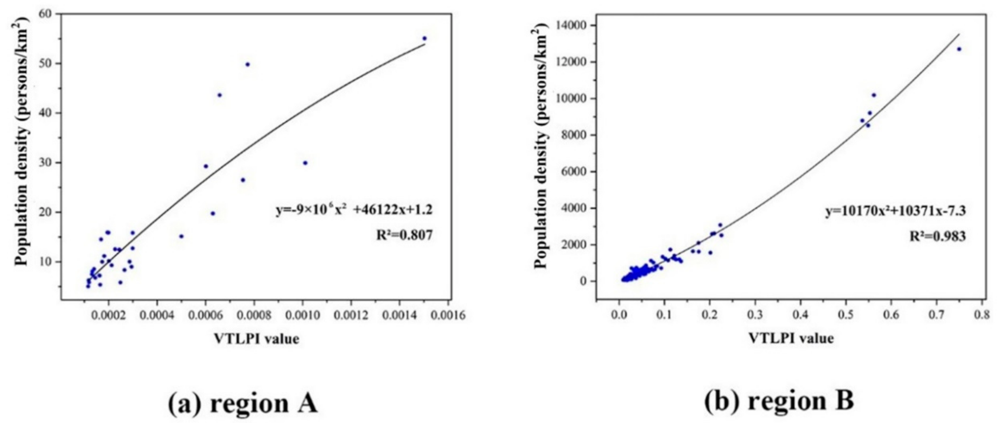
After the elevation correction in region A, the relationships between the population density and the averaged VTLPI values at the county level in the two regions are illustrated in Figure A2, and it can be described by the quadratic function after making a cross-validation comparison with other models such as linear, exponential and logarithmic models. Statistical evaluation of our proposed model indicated that the selected regression models were statistically significant based on F-test at less than 0.0001 (Table 1). The R2 in regions A and B are 0.807 and 0.983, respectively.
The MRE is 0.26 and the MdRE is 0.19, which might mean that the population density was accurately estimated with our models in most counties. The population density at the 250m grid level of Sichuan province in 2015 is shown in Figure 7, and it can be seen that the result accurately reflects the population diversity in Sichuan Province. The spatial distribution of the population was uneven and the population density decreased in turn in the east, south and west. The western mountainous areas were very sparsely populated in 2015 while the eastern plains and hilly areas were relatively much densely populated. The Chengdu City had the highest population density in Sichuan and several satellite cities around the Chengdu downtown, about 10 kilometers away from the city center, also had high population density. The population density had spatially decreased sharply from the inside to outside of the City.
3.2. Accuracy Assessment
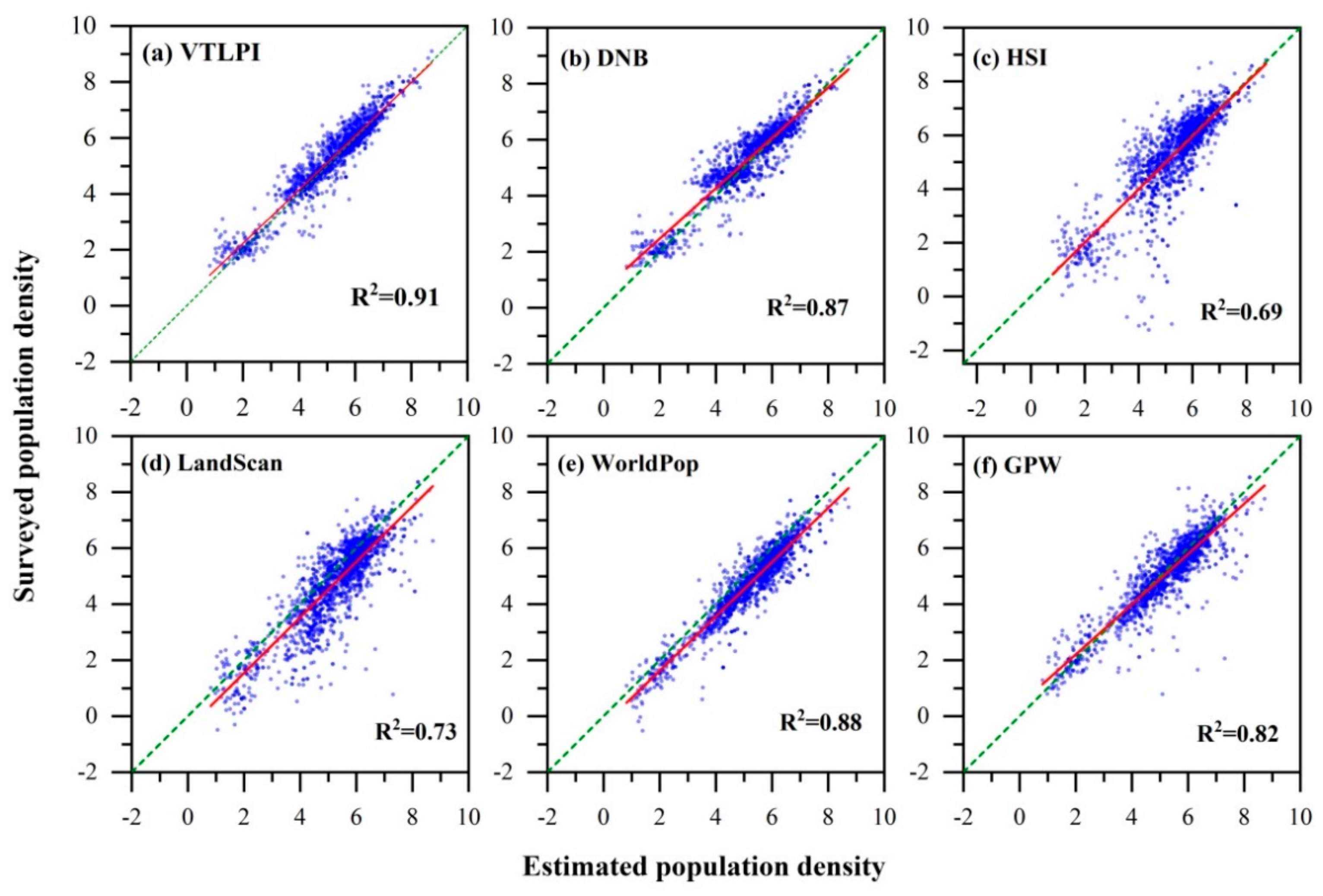
The sampling survey work was conducted in Sichuan Province in 2015 and the population data of totally 3285 townships were investigated and collected, among which 2000 townships and sub-districts were randomly selected for assessing the accuracy of our proposed model. The relationship between the VTLPI-modeled population density and sampling surveyed population density is illustrated in Figure 8a. The modeled population density well correlated with the census data and our model achieved a reasonable estimation of population density, both in the western mountainous area and the eastern plains and hilly area. When the sampling surveyed population density of the 2000 townships was used as reference, the determination coefficient of is 0.91, the RMSE is 212 person/km2, the MAR is 0.29 and the MdRE is 0.12.
3.3. Comparison with Other Methods
3.3.1. Comparative Analysis at the County and Township Levels
To fully evaluate the proposed index VTLPI, we selected two existing methods, DNB-based [26,38,72,73] and HSI-based [5] for comparison. The same input dataset and training samples of our VTLPI-based model were adopted to implement these two models, and the elevation correction was performed for each model. Comparative analysis of the three models (Table 2) indicated that all the three models had good performance ( ≥ 0.7), and our VTLPI-based model appears to be the best one with of 0.91 and RMSE of 206.46 person/km2. Moreover, the VTLPI-based estimate achieved the smallest MRE and MdRE—0.26, and, 0.19 respectively—which proved that the VTLPI-based model had the best performance in the estimation of population density at the county level among the three regression methods.
After building the three regression models using the same county-level census data, the sampling survey population data of 2000 townships and sub-districts were used to assess the performance of the three models (VTLPI-, DNB-, and HSI-based) and the three datasets, the LandScan (https://landscan.ornl.gov), WorldPop (https://www.worldpop.org/) and GPW (http://sedac.ciesin.columbia.edu/data/collection/gpw-v4).
Moreover, the model fittings between the estimated and the surveyed population density at the township level for the six population data products were examined for the purpose of comparison (Table 3, Figure 8). The VTLPI-based approach achieved significantly higher accuracy with the of 0.91 than the other five data products. It is clear that the VTLPI-based population data product has the best performance, and the RMSE, MAE, and MdRE are 212.31 person/km2, 0.29, and 0.12, respectively.
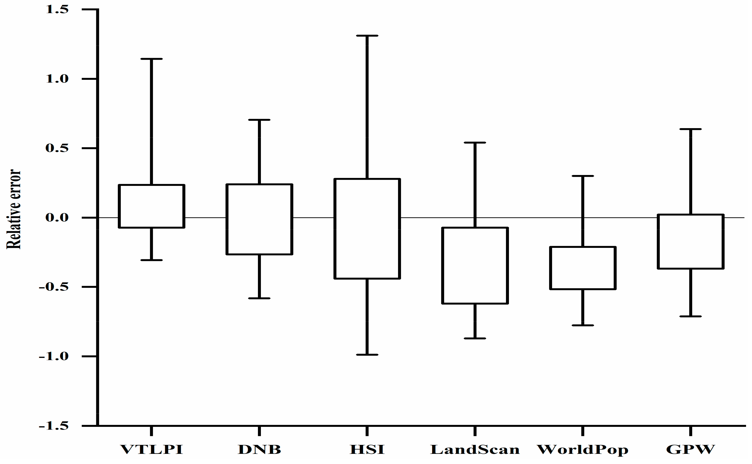
The box plot in Figure 9 showed the RE values of the modeled population density and the three population products. The lower whisker and upper whisker represent the 5th percentiles and the 95th percentiles, respectively. A quick visual check indicated that VTLPI-based estimation achieved a much better result than the other five results, and the relative errors lie in the second narrowest range. Although the WorldPop dataset achieved the narrowest RE distribution, it has obvious negative bias, which means underestimation of population density. The RE values of HSI- and DNB-based estimations have similar distributing patterns, but HSI-based estimation has the largest error range in the six estimations. It is also seen in Figure 9 that the population density in most townships was relatively underestimated in the LandScan, WorldPop, and GPW products.
3.3.2. Comparison of Specific Spatial Locations
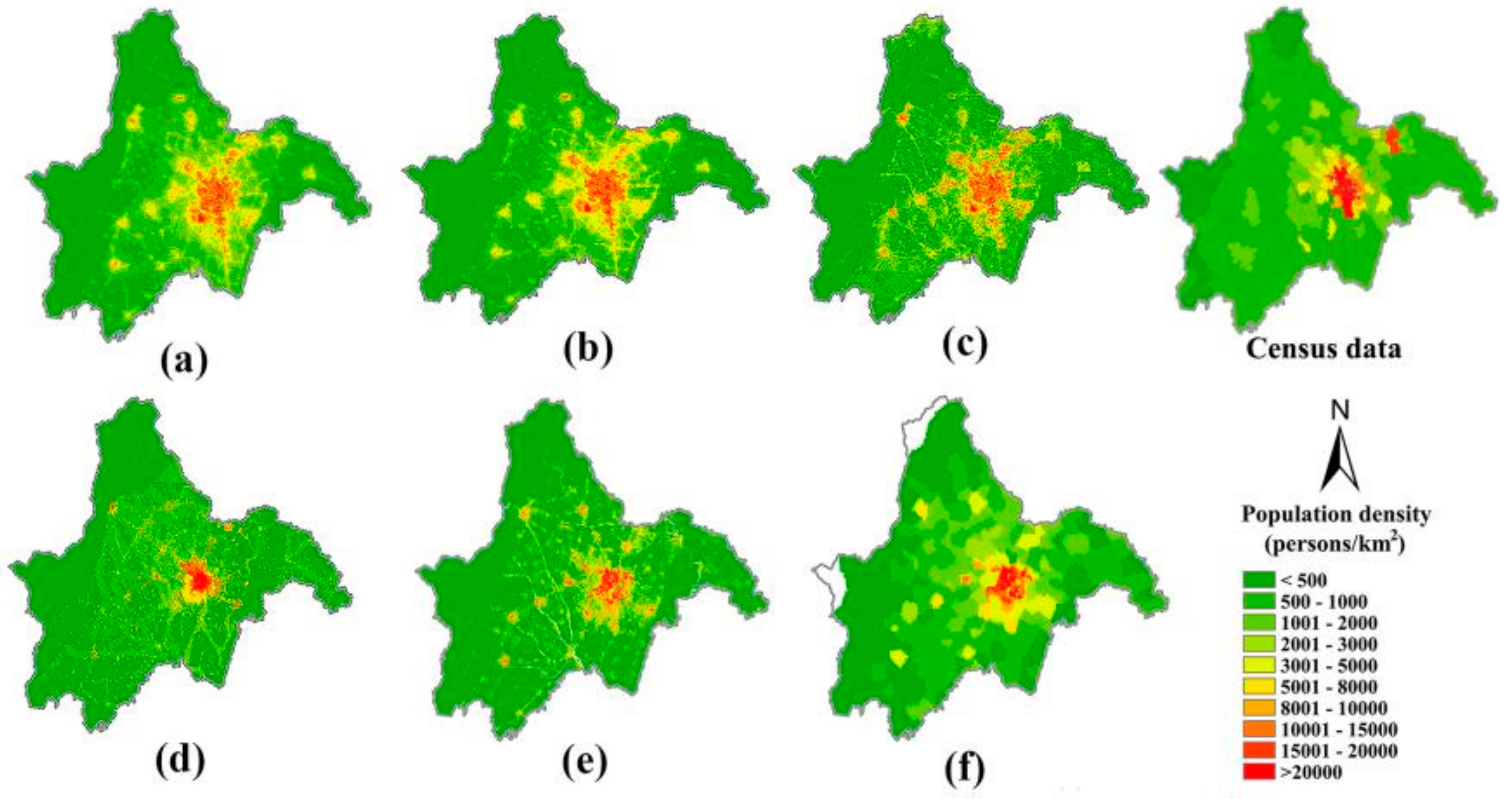
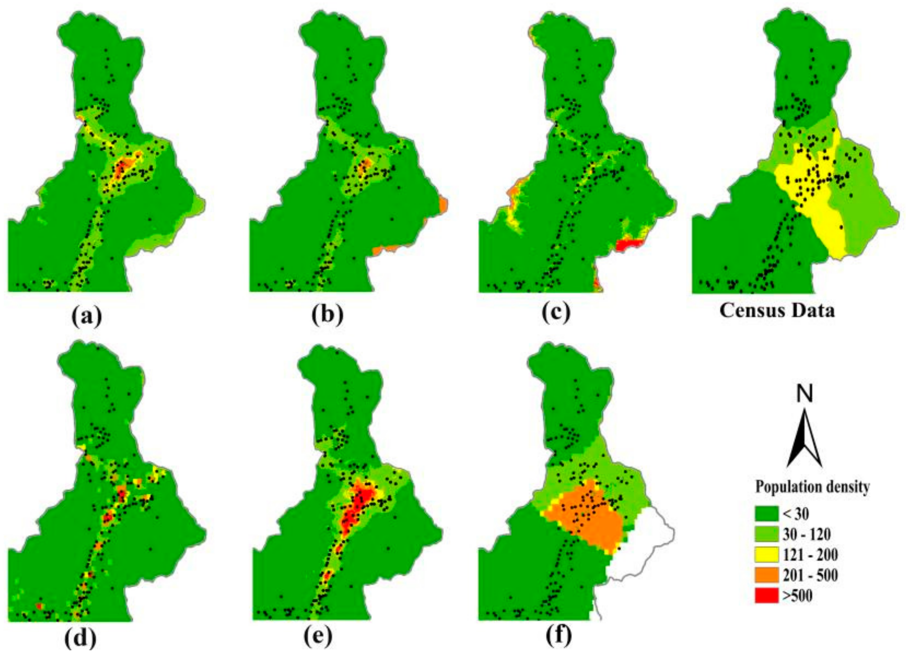
All the six population data products were re-projected into ACEA projection and resampled to 250 m images using the bilinear interpolation algorithm. It is seen in Figure 10 that compared with the LandScan, GPW, and WorldPop datasets, the population data products that were generated by the three regression models (Figure 10a–c) can offer larger spatial variations in the modeled population density in Chengdu City.
It can be seen that the VTLPI-based population density in the suburban areas is the highest and greater than 500 person/km2, which is consistent with the actual population distribution characterized by the census data (Figure 10). The suburban population density predicted by the other five products is relatively smaller. Two population datasets, LandScan and WorldPop, both using dasymetric mapping method, had similar spatial patterns of population density (e.g., areas with greater than 1000 person/km2). However, both the spatial distribution and the density values are obviously different from the actual population distribution in the Chengdu metropolitan area. Moreover, the population density of the two population products on both sides of the roads is abnormally large in these two data products. Compared with the LandScan data, the WorldPop data could provide more spatial details of population distribution. The GPW data had the lowest accuracy on the pixel scale because of the limitation of the areal weighting method that we already mentioned in the section of the introduction. The HSI-based model underestimated population density in the suburban areas, and the population distribution showed big variation in the rural areas, which is not the regular pattern of population distribution in Sichuan. Furthermore, HSI is particularly sensitive to the change of NDVI [57], leading to some unreasonable overestimation, especially in the areas with lower DNB values. As showed in Figure 10c, NDVI was unexpectedly small in the rural areas (e.g., on the side of the roads) and the estimated population density was over 1000 persons/km2. Similar phenomena appeared in bare mountains where the population density even exceeded that in some urban areas. Although the population density modeled by DNB was relatively reasonable in the rural areas, it could not reveal many details especially in urban core areas because of the limitation of DNB data such as blooming phenomenon. Among the three population data products estimated by VTLPI, HSI, and DNB, the population densities in the Shuangliu International Airport were the highest, 49,063; 176,406; and 124,029 persons/km2, respectively. It is obvious that VTLPI could effectively suppress overestimation caused by the excessive NTL values resulted from some external factors such as economic development level or special needs of light in some places (e.g., airport, large transportation hubs).
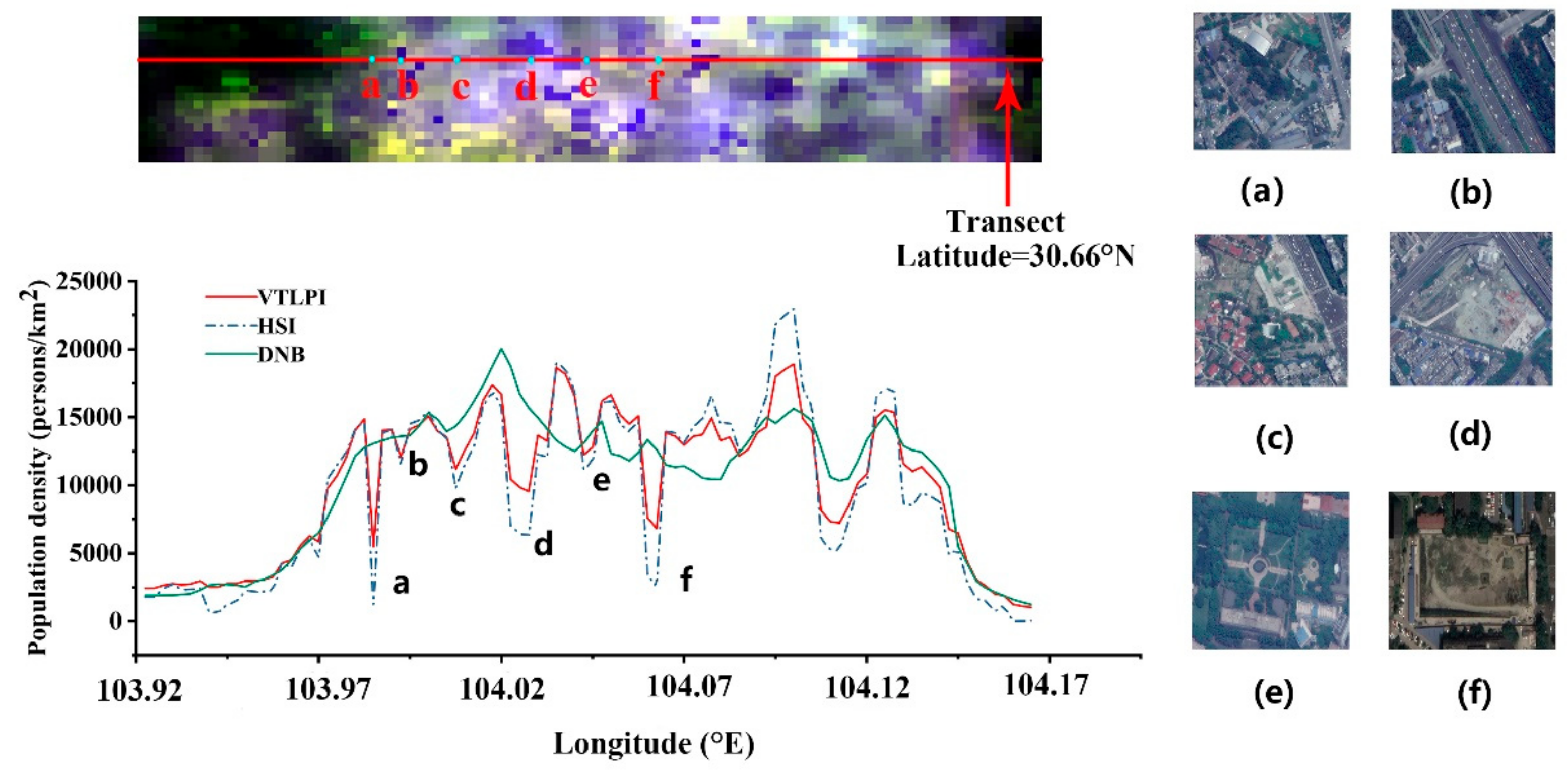
Three latitudinal profiles of the population density images estimated by the VTLPI-based, HSI-based, and DNB-based models were also created to conduct a comparative study (Figure A3). It can be seen that the trends of population density distribution along the profiles using the three regression models were quite similar. However, the DNB-estimated population density had smaller variability in the urban core area, and the population density was overestimated in some urban green spaces (Figure A3a–f). These areas were less populated but had higher light values affected by the blooming effect from adjacent pixels. The population density estimated using the VTLPI and HSI around these pixels obviously decreased. This indicated that the integration of LST and VI data could prevent the overestimation of population density derived from single DNB data in certain places.
The spatial distribution of population density in the Wenchuan County in Sichuan province is examined (Figure A4) and similar improvements in the estimation of population density were observed in this county. Details of the comparison are presented in Appendix A4.
4. Discussion
4.1. Performance of VTLPI for Population Estimation
Based on the assessment in Section 3, VTLPI-based estimation achieved a better result at county, town, and grid levels, and could offer a much richer spatial variation of population distribution in both rural and urban areas. The VTLPI-based model removed some drawbacks of DNB-based [38,72,73] and HSI-based [5,20] or those combined methods, in which the booming effect of NTL, economic developing levels, and bright facilities (e.g., airports, overpasses) can lead to over- or under-estimation of population density. The effect of using VTLPI to estimate the population mainly lies in two points, adding LST information and square root transformation of the light data. Compared with HSI and DNB, the VTLPI-based regression model significantly inhibits the overestimation in airport areas and urban green areas (Figure 10 and Figure A3). However, both VTLPI and HSI use VI as an essential variable for population estimation, in which the premise is that vegetation coverage and NDVI values are much smaller in towns and villages, but the NDVI values in human settlements in arid regions such as deserts and oasis are even larger than the bare lands. Consequently, the proposed method might lead to overestimation in the oasis and desert areas. We also found that our VTLPI-based model might overestimate the population density at some factories with high temperatures, such as power plants.
Moreover, this study also proved that the elevation correction could significantly improve the accuracy of population density estimation. After the elevation correction in Region A in our study, the determinant coefficient for the VTLPI-based regression model was enhanced from 0.52 to 0.80, and RMSE was declined from 8.47 to 5.54. Most of the human settlements are in lower elevations [5,14], thus the correction is necessary for population estimation, especially in high altitudes or mountains.
Future work may incorporate some social sensing data such as POI data and global navigation satellite system (GNSS) tracking data into the modeling of population density to create dynamic population distribution, termed ambient population data, to meet the requirements of some applications such as earthquake loss assessment.
4.2. Regression Analysis Versus Dasymetric Mapping
Regression analysis and dasymetric mapping are two mainstream methods for population estimation over a large area. Speaking generally, in the case of having other auxiliary data and sufficient labor and material resources, dasymetric mapping can be used to obtain a finer scale population density. It can more easily combine multi-source remote sensing data, and various social sensing data, such as point-of-interest (POI) points, GNSS positioning data, etc. However, these data usually can only be obtained at small scales (such as a certain city). Therefore, when the dasymetric mapping is used for large-scale mapping, it may be less accurate in some areas due to the lack of detailed and complete auxiliary data. As shown in the Figure 10e, although the resolution of WorldPop dataset (https://www.worldpop.org/) is 100 × 100 m, it can be seen that in some areas, the population distribution presenting regular blocks (the scale much larger than 100 m), which is not consistent with the actual spatial distribution of the population. This may be directly affected by the auxiliary data with a relatively coarse resolution or grouping population numbers directly into administrative units. In addition, the process of determining the weights of different variables is often very complicated, and sometimes the weights do not conform to the patterns of population distribution. For example, the distance from the road network is often an important variable in the dasymetric mapping. As can be seen in Figure 10d,e, the population density obtained by the dasymetric mapping is significantly higher nearby the roads. More and more studies used random forest algorithm to get the weight to redistribute the population [20,23,74,75], but this method still requires further mechanistic explanation.
Compared with the dasymetric mapping, regression analysis relies on statistical models that are more suitable for population mapping in cases where auxiliary data are difficult to obtain, and it is much easier to be implemented when the derivatives from remotely sensed imagery are used in the estimation of population density. For instance, the proposed VTLPI from multi-sensor data in this study can be well incorporated into the modeling of the population density of Sichuan Province. However, it is difficult for regression analysis to include some social sensing data into the estimation of the population because of their spatially discrete distribution.
This study also finds that the integration of land cover data with VIIRS DNB data did not significantly improve the accuracy of population estimation, different from some previous research [10,30]. That might be owed to the fact that the urban land covers were usually classified into one class, and the land cover data could not provide enough variations inside a city. For example, the FROM-GLC data simply classified almost the entire Chengdu City into the impervious surface. Moreover, land cover products often failed to reflect small village information, which leads to lower accuracy of rural population estimation.
Due to the above problems, it is necessary to integrate social sensing data and remote sensing data for population estimation. An effective population mapping method is to combine the dasymetric mapping with the regression analysis. First, in large areas (e.g., provinces) which lack sufficient auxiliary data, using remote sensing data to construct regression models to obtain coarse gridded population density. Second, the dasymetric mapping method can be used to further refine the previously obtained population density grids in a specific city with sufficient auxiliary data (e.g., POI data).
5. Conclusions
This study presented a robust mapping approach for population distribution based on multi-sensor remote sensing data. A new index VTLPI combining the NPP/VIIRS DNB, MODIS NDVI, and MODIS LST data was proposed and used to build the regression model for the estimation of the 250 m gridded population density. The proposed approach aims to avoid the overestimation of population density in urban areas and underestimation in suburbs and rural villages. A case study with our proposed method was implemented using the data of Sichuan Province, China in 2015. The results indicated that the estimated 250 m population density outperformed the results from DNB-based and HSI-based models as well as the three population datasets, LandScan data, WorldPop data, and GPW. The mean relative error and median absolute relative error at the town level are 0.29 and 0.12 respectively, and the RMSE is 212.31 persons/ when the census data of 2000 townships and sub-districts were used as reference. The results also demonstrated that the VTLPI-estimated population distribution had more spatial variations and richer information in both urban and rural areas, and could prevent the underestimation in the rural areas well, and the overestimation in the urban green spaces and facilities with a high density of lamps (e.g., airports, overpasses).
Future work may focus on incorporating multi-sensor data with social sensing data (e.g., POI) to estimate the dynamic variations of population distribution at a grid spatial resolution. We will extend the validation work to other areas such as Gansu and Xinjiang, where earthquake risk is relatively high and household or street census data should be collected to verify our VTLPI-based model better.
Author Contributions
X.Z. and P.L. conceived and designed the study. P.L. designed and implemented the methods, analyzed the data and performed the experiments. J.C. and Q.S. collected in-situ data and analyzed the census data.
Funding
This research was jointly funded by National Key Research and Development Program of China (grant no. 2017YFC1500902) and by the Xinjiang Production and Construction Corps (grant no. 2017DB005).
Conflicts of Interest
The authors declare no conflict of interest.
Appendix A
Appendix A1. Determination of Parameter C
Figure A1.
Relationship between and D. It can be seen that the correlative coefficient achieves maximum when approximately 2500m is assigned to D.
Figure A1.
Relationship between and D. It can be seen that the correlative coefficient achieves maximum when approximately 2500m is assigned to D.

Appendix A2. Regression Analysis in Region A and B
Figure A2.
Modeling of the relationship between the corrected VTLPI and county-level census data in the two regions of the study area. The dots in (a) represent all the counties at region A and the dots in (b) represent those counties at region B.
Figure A2.
Modeling of the relationship between the corrected VTLPI and county-level census data in the two regions of the study area. The dots in (a) represent all the counties at region A and the dots in (b) represent those counties at region B.

Appendix A3. The Latitudinal Transect in the Chengdu City
Figure A3.
The color composite images (population density estimated using VTLPI, HSI, and DNB as R, G, and B), and the latitudinal transects of the three population density in Chengdu City. (a–f) images on the right are Google images in 2015 corresponding to the locations in latitudinal transects. The blue dots on the transect line corresponds to the six positions from a to f.

Appendix A4. Comparison of Population Density in the Wenchuan County
It can be seen in Figure A4 that the population density of the majority of the Wenchuan township was greater than 30 persons/ based on the VTLPI-estimated population and WorldPop products, which is well consistent with the census data. However, the population density of the WorldPop data in the central areas of the Wenchuan town was relatively higher than the VTLPI-modeled result, and the areas with a population density above 500 persons/ are much larger than the VTLPI-estimated, which is not consistent with the actual population distribution in the census data. The other four population data products had significant underestimations in the central Wenchuan town and its suburbs (Figure A4b–d,f). It proved that our VTLPI-based model could enhance human activity information even in small habitats. Among the three population datasets, the LandScan and GPW products were not convincing in the Wenchuan area while the WorldPop dataset could provide more details in urban areas and reveal information of the small villages compared with the other two products (Figure A4e). In sum, our proposed VTLPI-based model can achieve a better estimation of the population density in the Wenchuan county, both in urban and rural areas.
Figure A4.
Census data map and six population data products in the Wenchuan town generated by the three regression models, (a) VTLPI, (b) DNB, (c) HSI, and the three products, (d) LandScan, (e) WorldPop, and (f) GPW. The dots represent the central location of the villages in the Wenchuan County.
Figure A4.
Census data map and six population data products in the Wenchuan town generated by the three regression models, (a) VTLPI, (b) DNB, (c) HSI, and the three products, (d) LandScan, (e) WorldPop, and (f) GPW. The dots represent the central location of the villages in the Wenchuan County.

References
- Hay, S.I.; Noor, A.M.; Nelson, A.; Tatem, A.J. The accuracy of human population maps for public health application. Trop. Med. Int. Health 2005, 10, 1073–1086. [Google Scholar] [CrossRef] [PubMed]
- Ahola, T.; Virrantaus, K.; Krisp, J.M.; Hunter, G.J.; Ahola, T.; Virrantaus, K.; Krisp, J.M.; Hunter, G.J. A spatio-Temporal population model to support risk assessment and damage analysis for decision-making. Int. J. Geogr. Inf. Sci. 2007, 21, 935–953. [Google Scholar] [CrossRef]
- Aubrecht, C.; Özceylan, D.; Steinnocher, K.; Freire, S. Multi-level geospatial modeling of human exposure patterns and vulnerability indicators. Nat. Hazards 2013, 68, 147–163. [Google Scholar] [CrossRef]
- Jia, P.; Qiu, Y.; Gaughan, A.E. A fine-scale spatial population distribution on the High-resolution Gridded Population Surface and application in Alachua County, Florida. Appl. Geogr. 2014, 50, 99–107. [Google Scholar] [CrossRef]
- Yang, X.; Yue, W.; Gao, D. Spatial improvement of human population distribution based on multi-sensor remote-sensing data: An input for exposure assessment. Int. J. Remote Sens. 2013, 34, 5569–5583. [Google Scholar] [CrossRef]
- Yang, X.; Huang, Y.; Dong, P.; Jiang, D.; Liu, H. An updating system for the gridded population database of china based on remote sensing, GIS and spatial database technologies. Sensors 2009, 9, 1128–1140. [Google Scholar] [CrossRef]
- Roy Chowdhury, P.K.; Maithani, S.; Dadhwal, V.K. To Estimation of urban population in Indo-Gangetic Plains using night-time OLS data. Int. J. Remote Sens. 2012, 33, 2498–2515. [Google Scholar] [CrossRef]
- Tian, Y.; Yue, T.; Zhu, L.; Clinton, N. Modeling population density using land cover data. Ecol. Model. 2005, 189, 72–88. [Google Scholar] [CrossRef]
- Elvidge, C.D.; Baugh, K.E.; Kihn, E.A.; Kroehl, H.W.; Davis, E.R.; Davis, C.W.; Baugh, K.E.; Kihn, E.A.; Kroehl, H.W.; Davis, E.R. Relation between satellite observed visible-near infrared emissions, population, economic activity and electric power consumption. Int. J. Remote Sens. 1997, 18, 1373–1379. [Google Scholar] [CrossRef]
- Tan, M.; Li, X.; Li, S.; Xin, L.; Wang, X.; Li, Q.; Li, W.; Li, Y.; Xiang, W. Modeling population density based on nighttime light images and land use data in China. Appl. Geogr. 2018, 90, 239–247. [Google Scholar] [CrossRef]
- Chen, K.; McAneney, J.; Blong, R.; Leigh, R.; Hunter, L.; Magill, C. Defining area at risk and its effect in catastrophe loss estimation: A dasymetric mapping approach. Appl. Geogr. 2004, 24, 97–117. [Google Scholar] [CrossRef]
- Zoraghein, H.; Leyk, S.; Ruther, M.; Butten, B.P. Exploiting temporal information in parcel data to re fi ne small area population estimates. Comput. Environ. Urban Syst. 2016, 58, 19–28. [Google Scholar] [CrossRef]
- Zoraghein, H.; Leyk, S. Enhancing areal interpolation frameworks through dasymetric refinement to create consistent population estimates across censuses Enhancing areal interpolation frameworks through. Int. J. Geogr. Inf. Sci. 2018, 32, 1948–1976. [Google Scholar] [CrossRef] [PubMed]
- Zoraghein, H.; Leyk, S. Data-enriched interpolation for temporally consistent population compositions. GISci. Remote Sens. 2019, 56, 430–461. [Google Scholar] [CrossRef]
- Zandbergen, P.A.; Ignizio, D.A. Comparison of Dasymetric Mapping Techniques for Small-Area Population Estimates. Cartogr. Geogr. Inf. Sci. 2010, 37, 199–214. [Google Scholar] [CrossRef]
- Balk, D.; Yetman, G. The Global Distribution of Population: Evaluating the Gains in Resolution Refinement; Columbia University Press: New York, NY, USA, 2004; Available online: https://sedac.ciesin.columbia.edu/downloads/docs/gpw-v3/gpw3_documentation_final.pdf (accessed on 8 November 2019).
- Doxsey-Whitfield, E.; Macmanus, K.; Adamo, S.B.; Pistolesi, L.; Squires, J.; Borkovska, O.; Baptista, S.R.; Macmanus, K.; Adamo, S.B.; Pistolesi, L.; et al. Taking Advantage of the Improved Availability of Census Data: A First Look at the Gridded Population of the World, Version 4. Pap. Appl. Geogr. 2015, 1, 226–234. [Google Scholar] [CrossRef]
- Bhaduri, B.; Bright, E.; Coleman, P.; Urban, M.L. LandScan USA: A high-resolution geospatial and temporal modeling approach for population distribution and dynamics. GeoJournal 2007, 69, 103–117. [Google Scholar] [CrossRef]
- Mennis, J. Generating Surface Models of Population Using Dasymetric Mapping. Prof. Geogr. 2003, 55, 31–42. [Google Scholar]
- Ye, T.; Zhao, N.; Yang, X.; Ouyang, Z.; Liu, X.; Chen, Q.; Hu, K.; Yue, W.; Qi, J.; Li, Z.; et al. Science of the Total Environment Improved population mapping for China using remotely sensed and points-of-interest data within a random forests model. Sci. Total Environ. 2019, 658, 936–946. [Google Scholar] [CrossRef]
- Yue, T.X.; Wang, Y.A.; Chen, S.P.; Liu, J.Y.; Qiu, D.S.; Deng, X.Z.; Liu, M.L.; Tian, Y.Z. Numerical simulation of population distribution in China. Popul. Environ. 2003, 25, 141–163. [Google Scholar] [CrossRef]
- Sutton, P.C.; Elvidge, C.; Obremski, T. Building and Evaluating Models to Estimate Ambient Population Density. Photogramm. Eng. Remote Sens. 2003, 69, 545–553. [Google Scholar] [CrossRef]
- Gaughan, A.E.; Stevens, F.R.; Linard, C.; Jia, P.; Tatem, A.J. High Resolution Population Distribution Maps for Southeast Asia in 2010 and 2015. PLoS ONE 2015, 8, e55882. [Google Scholar] [CrossRef] [PubMed]
- Sutton, P.C.; Taylor, M.J.; Elvidge, C.D. Using DMSP OLS Imagery to Characterize Urban Populations in Developed and Developing Countries. In Remote Sensing of Urban and Suburban Areas; Springer: Dordrecht, The Netherlands, 2010; pp. 329–348. [Google Scholar]
- Gallego, F.J. A population density grid of the European Union. Popul. Environ. 2010, 31, 460–473. [Google Scholar] [CrossRef]
- Liu, X.; Zhu, X.; Pan, Y.; Ma, Y.; Li, T.; Chen, S. Mapping population distribution by integrating night-time light satellite imagery and land-cover data. In Proceedings of the International Geoscience and Remote Sensing Symposium (IGARSS), Milan, Italy, 26–31 July 2015; IEEE: Piscataway, NJ, USA, 2015; pp. 2186–2189. [Google Scholar]
- Linard, C.; Gilbert, M.; Snow, R.W.; Noor, A.M.; Tatem, A.J. Population distribution, settlement patterns and accessibility across Africa in 2010. PLoS ONE 2012, 7, e31743. [Google Scholar] [CrossRef]
- Sutton, P.; Roberts, D.; Elvidge, C.; Baugh, K. Census from Heaven: An estimate of the global human population using night-time satellite imagery. Int. J. Remote Sens. 2001, 22, 3061–3076. [Google Scholar] [CrossRef]
- Jing, X.; Shao, X.; Cao, C.; Xiaodong, L.Y. Comparison between the Suomi-NPP Day-Night Band and DMSP-OLS for Correlating Socio-Economic Variables at the Provincial Level in China. Remote Sens. 2016, 8, 17. [Google Scholar] [CrossRef]
- Bagan, H.; Yamagata, Y. Analysis of urban growth and estimating population density using satellite images of nighttime lights and land-use and population data. GISci. Remote Sens. 2015, 52, 765–780. [Google Scholar]
- Small, C.; Pozzi, F.; Elvidge, C.D. Spatial analysis of global urban extent from DMSP-OLS night lights. Remote Sens. Environ. 2005, 96, 277–291. [Google Scholar] [CrossRef]
- Imhoff, M.; Lawrence, W.T.; Elvidge, C.D. A technique for using composite DMSP/OLS “City Lights” satellite data to map urban area. Remote Sens. Environ. 1997, 61, 361–370. [Google Scholar] [CrossRef]
- Zhang, X.; Li, P. A temperature and vegetation adjusted NTL urban index for urban area mapping and analysis. ISPRS J. Photogramm. Remote Sens. 2018, 135, 93–111. [Google Scholar] [CrossRef]
- Miller, S.D.; Turner, R.E. A dynamic lunar spectral irradiance data set for NPOESS/VIIRS day/night band night time environmental applications. IEEE Trans. Geosci. Remote Sens. 2009, 47, 2316–2329. [Google Scholar] [CrossRef]
- Chen, Z.; Yu, B.; Hu, Y.; Huang, C.; Shi, K.; Wu, J. Estimating House Vacancy Rate in Metropolitan Areas Using NPP-VIIRS Nighttime Light Composite Data. IEEE J. Sel. Top. Appl. Earth Obs. Remote Sens. 2015, 8, 2188–2197. [Google Scholar] [CrossRef]
- Wang, X.; Rafa, M.; Moyer, J.D.; Li, J.; Scheer, J.; Sutton, P. Estimation and Mapping of Sub-National GDP in Uganda Using NPP-VIIRS Imagery. Remote Sens. 2019, 11, 163. [Google Scholar] [CrossRef]
- Chen, X.; Nordhaus, W. A test of the new VIIRS lights data set: Population and economic output in Africa. Remote Sens. 2015, 7, 4937–4947. [Google Scholar] [CrossRef]
- Amaral, S.; Câmara, G.; Monteiro, A.M.V.; Quintanilha, J.A.; Elvidge, C.D. Estimating population and energy consumption in Brazilian Amazonia using DMSP night-time satellite data. Comput. Environ. Urban Syst. 2005, 29, 179–195. [Google Scholar] [CrossRef]
- Dong, N.; Yang, X.; Cai, H.; Wang, L. A novel method for simulating urban population potential based on urban patches: A case study in Jiangsu Province, China. Sustainability 2015, 7, 3984–4003. [Google Scholar] [CrossRef]
- Yu, B.; Lian, T.; Huang, Y.; Yao, S.; Ye, X.; Chen, Z.; Yang, C.; Wu, J. Integration of nighttime light remote sensing images and taxi GPS tracking data for population surface enhancement Bailang. Int. J. Geogr. Inf. Sci. 2019, 33, 687–706. [Google Scholar] [CrossRef]
- Lu, D.; Tian, H.; Zhou, G.; Ge, H. Regional mapping of human settlements in southeastern China with multisensor remotely sensed data. Remote Sens. Environ. 2008, 112, 3668–3679. [Google Scholar] [CrossRef]
- Maithani, P.K.R.C.S. Monitoring Growth of Built-up areas in Indo-Gangetic Plain using Multi-sensor Remote Sensing Data. J. Indian Soc. Remote Sens. 2010, 38, 291–300. [Google Scholar]
- Yu, B.; Tang, M.; Wu, Q.; Yang, C.; Deng, S.; Shi, K.; Peng, C.; Wu, J.; Chen, Z. Urban built-up area extraction from log-transformed NPP-VIIRS nighttime light composite data. IEEE Geosci. Remote Sens. Lett. 2018, 15, 1279–1283. [Google Scholar] [CrossRef]
- Guo, W.; Lu, D.; Wu, Y.; Zhang, J. Mapping impervious surface distribution with integration of SNNP VIIRS-DNB and MODIS NDVI Data. Remote Sens. 2015, 7, 12459–12477. [Google Scholar] [CrossRef]
- Gorelick, N.; Hancher, M.; Dixon, M.; Ilyushchenko, S.; Thau, D.; Moore, R. Remote Sensing of Environment Google Earth Engine: Planetary-scale geospatial analysis for everyone. Remote Sens. Environ. 2017, 202, 18–27. [Google Scholar] [CrossRef]
- Lobell, D.B.; Thau, D.; Seifert, C.; Engle, E.; Little, B. Remote Sensing of Environment A scalable satellite-based crop yield mapper. Remote Sens. Environ. 2015, 164, 324–333. [Google Scholar] [CrossRef]
- Xiong, J.; Thenkabail, P.S.; Gumma, M.K.; Teluguntla, P.; Poehnelt, J.; Congalton, R.G.; Yadav, K.; Thau, D. ISPRS Journal of Photogrammetry and Remote Sensing Automated cropland mapping of continental Africa using Google Earth Engine cloud computing. ISPRS J. Photogramm. Remote Sens. 2017, 126, 225–244. [Google Scholar] [CrossRef]
- Goldblatt, R.; You, W.; Hanson, G.; Khandelwal, A.K. Detecting the Boundaries of Urban Areas in India: A Dataset for Pixel-Based Image Classification in Google Earth Engine. Remote Sens. 2016, 8, 634. [Google Scholar] [CrossRef]
- Chen, J.; Chen, J.; Liao, A.; Cao, X.; Chen, L.; Chen, X.; He, C.; Han, G.; Peng, S.; Lu, M.; et al. ISPRS Journal of Photogrammetry and Remote Sensing Global land cover mapping at 30 m resolution: A POK-based operational approach. ISPRS J. Photogramm. Remote Sens. 2015, 103, 7–27. [Google Scholar] [CrossRef]
- Chen, Z.; Yu, B.; Song, W.; Liu, H.; Wu, Q.; Shi, K.; Wu, J. A New Approach for Detecting Urban Centers and Their Spatial Structure With Nighttime Light Remote Sensing. IEEE Trans. Geosci. Remote Sens. 2017, 55, 6305–6319. [Google Scholar] [CrossRef]
- Li, X.; Xu, H.; Chen, X.; Li, C. Potential of NPP-VIIRS nighttime light imagery for modeling the regional economy of China. Remote Sens. 2013, 5, 3057–3081. [Google Scholar] [CrossRef]
- Bhandari, S.; Phinn, S.; Gill, T.; Bhandari, S.; Phinn, S.; Gill, T. Assessing viewing and illumination geometry effects on the MODIS vegetation index (MOD13Q1) time series: Implications for monitoring phenology and disturbances in forest communities in. Int. J. Remote Sens. 2011, 32, 7513–7538. [Google Scholar] [CrossRef]
- Huete, A.; Didan, K.; Miura, T.; Rodriguez, E.P.; Gao, X.; Ferreira, L.G. Overview of the radiometric and biophysical performance of the MODIS vegetation indices. Remote Sens. Environ. 2002, 83, 195–213. [Google Scholar] [CrossRef]
- Zhao, L.; Lee, X.; Smith, R.B.; Oleson, K. Strong contributions of local background climate to urban heat islands. Nature 2014, 511, 216–219. [Google Scholar] [CrossRef] [PubMed]
- Santillan, J.R.; Makinano-santillan, M. Vertical accuracy assessment of 30-m resolution alos, aster, and srtm global dems over northeastern mindanao, philippines. Int. Arch. Photogramm. Remote Sens. Spat. Inf. Sci. 2016, 41, 149–156. [Google Scholar] [CrossRef]
- Gong, P.; Wang, J.; Yu, L.; Zhao, Y.; Zhao, Y.; Liang, L.; Yu, L.; Wang, L.; Liu, X.; Shi, T.; et al. Finer resolution observation and monitoring of global land cover: First mapping results with Landsat TM and ETM + data. Int. J. Remote Sens. 2013, 34, 2607–2654. [Google Scholar] [CrossRef]
- Ma, T.; Zhou, C.; Pei, T.; Haynie, S.; Fan, J. Responses of Suomi-NPP VIIRS-derived nighttime lights to socioeconomic activity in Chinas cities. Remote Sens. Lett. 2014, 5, 165–174. [Google Scholar] [CrossRef]
- Weng, Q.; Lu, D.; Schubring, J. Estimation of land surface temperature – vegetation abundance relationship for urban heat island studies. Remote Sens. Environ. 2004, 89, 467–483. [Google Scholar] [CrossRef]
- Lu, D.; Weng, Q.; Li, G. Residential population estimation using a remote sensing derived impervious surface approach. Int. J. Remote Sens. 2006, 27, 3553–3570. [Google Scholar] [CrossRef]
- Hao, R.; Yu, D.; Sun, Y.; Cao, Q.; Liu, Y.; Liu, Y. Integrating multiple source data to enhance variation and weaken the blooming effect of DMSP-OLS light. Remote Sens. 2015, 7, 1422–1440. [Google Scholar] [CrossRef]
- Heinl, M.; Hammerle, A.; Tappeiner, U.; Leitinger, G. Determinants of urban-rural land surface temperature differences—A landscape scale perspective. Landsc. Urban Plan. 2015, 134, 33–42. [Google Scholar] [CrossRef]
- Du, Y.; Xie, Z.; Zeng, Y.; Shi, Y.; Wu, J. Impact of urban expansion on regional tempera- ture change in the Yangtze River Delta. J. Geogr. Sci. 2007, 17, 387–389. [Google Scholar] [CrossRef]
- Li, J.; Song, C.; Cao, L.; Zhu, F.; Meng, X.; Wu, J. Remote Sensing of Environment Impacts of landscape structure on surface urban heat islands: A case study of Shanghai, China. Remote Sens. Environ. 2011, 115, 3249–3263. [Google Scholar] [CrossRef]
- Price, J.C. Using spatial context in satellite data to infer regional scale evapotranspiration. IEEE Trans. Geosci. Remote Sens. 1990, 28, 940–948. [Google Scholar] [CrossRef] [Green Version]
- Yue, W.; Xu, J.; Tan, W.; Xu, L. The relationship between land surface temperature and NDVI with remote sensing: Application to Shanghai Landsat 7 ETM + data. Int. J. Remote Sens. 2007, 28, 3205–3226. [Google Scholar] [CrossRef]
- Lambin, E.F.; Ehrlich, D. Land-cover Changes in Sub-Saharan Africa (1982–1991): Application of a Change Index Based on Remotely Sensed Surface Temperature and Vegetation Indices at a Continental Scale. Remote Sens. Environ. 1997, 61, 181–200. [Google Scholar] [CrossRef]
- Melesse, A.M.; Jordan, J.D. Spatially distributed watershed mapping and modeling: Thermal maps and vegetation indices to enhance land cover and surface microclimate mapping: Part 1. J. Spat. Hydrol. 2003, 3, 1–29. [Google Scholar]
- Lambin, E.F.; Ehrlich, D. Combining vegetation indices and surface temperature for land-cover mapping at broad spatial scales. Int. J. Remote Sens. 1995, 16, 573–579. [Google Scholar] [CrossRef]
- Lambin, E.F.; Ehrlich, D. The surface temperature-vegetation index space for land cover and land-cover change analysis. Int. J. Remote Sens. 1996, 17, 463–487. [Google Scholar] [CrossRef]
- Small, C.; Elvidge, C.D.; Baugh, K. Mapping Urban Structure and Spatial Connectivity with VIIRS and OLS Night Light Imagery. In Proceedings of the Joint Urban Remote Sensing Event 2013, São Paulo, Brazil, 21–23 April 2013; IEEE; pp. 230–233. [Google Scholar]
- Dong, P.; Ramesh, S.; Nepali, A. Evaluation of small-area population estimation using LiDAR, Landsat TM and parcel data. Int. J. Remote Sens. 2010, 31, 5571–5586. [Google Scholar] [CrossRef]
- Gao, B.; Huang, Q.; He, C.; Ma, Q. Dynamics of Urbanization Levels in China from 1992 to 2012: Perspective from DMSP/OLS Nighttime Light Data. Remote Sens. 2015, 7, 1721–1735. [Google Scholar] [CrossRef] [Green Version]
- Zhou, Y.; Smith, S.J.; Elvidge, C.D.; Zhao, K.; Thomson, A.; Imhoff, M. A cluster-based method to map urban area from DMSP/OLS nightlights. Remote Sens. Environ. 2014, 147, 173–185. [Google Scholar] [CrossRef]
- Stevens, F.R.; Gaughan, A.E.; Linard, C.; Tatem, A.J. Disaggregating Census Data for Population Mapping Using Random Forests with Remotely-Sensed and Ancillary Data. PLoS ONE 2015, 10, e0107042. [Google Scholar] [CrossRef]
- Gaughan, A.E.; Stevens, F.R.; Huang, Z.; Nieves, J.J.; Sorichetta, A.; Lai, S.; Ye, X.; Linard, C.; Hornby, G.M.; Hay, S.I.; et al. Spatiotemporal patterns of population in mainland China, 1990 to 2010. Sci. DATA 2016, 3, 160005. [Google Scholar] [CrossRef] [PubMed]
Figure 1.
Latitudinal transects of DNB (a) and SQRT DNB (b) for the Chengdu City (left column) and the Wenchuan county (right column) along the transect line in the top RGB color composite images (R=DNB, G=SQRT DNB, and B= NDVI). The bottom curves indicate more variations in the areas with low NTL values after the transformation.

Figure 2.
Color composite images (R=LST, G=DNB, B=NDVI) (top) and latitudinal transects (bottom) in the Chengdu City, China. It is seen that the NDVI values decreased at the locations of A, B, and C. The white dots on the transect line corresponds to the three locations A, B, and C.
Figure 2.
Color composite images (R=LST, G=DNB, B=NDVI) (top) and latitudinal transects (bottom) in the Chengdu City, China. It is seen that the NDVI values decreased at the locations of A, B, and C. The white dots on the transect line corresponds to the three locations A, B, and C.

Figure 3.
Color composite images (R=DNB, G=Urban percentage and B=VTLPI) (top) and latitudinal transects (bottom) in Chengdu City, China.
Figure 3.
Color composite images (R=DNB, G=Urban percentage and B=VTLPI) (top) and latitudinal transects (bottom) in Chengdu City, China.

Figure 4.
Location in China (a) and the elevation map of Sichuan Province (b). Region A includes the counties bounded with the black line, and Region B is composed of the rest counties of Sichuan.
Figure 4.
Location in China (a) and the elevation map of Sichuan Province (b). Region A includes the counties bounded with the black line, and Region B is composed of the rest counties of Sichuan.

Figure 5.
Correlation between the average elevation and population density of 37 counties in Region A.
Figure 5.
Correlation between the average elevation and population density of 37 counties in Region A.

Figure 6.
Scatterplots between the VTLPI, HSI, and DNB values and the county-level population density before (top) and after (bottom) the elevation correction. The solid line indicates the correlative analysis for the total counties, the dash line for the region A, and the short dash line for region B.

Figure 7.
Modeled population density at 250m grid cell (persons/) in Sichuan in 2015.

Figure 8.
Scatterplots of the estimated and the census population density at the township level. A natural logarithm transformation was performed for the population density data.
Figure 8.
Scatterplots of the estimated and the census population density at the township level. A natural logarithm transformation was performed for the population density data.

Figure 9.
Box plot of RE of the six estimated population density at the township level.

Figure 10.
Census data map and six population data products of the Chengdu City generated by the three regression models, (a) VTLPI, (b) DNB, (c) HSI, and the three products, (d) LandScan, (e) WorldPop, and (f) GPW.
Figure 10.
Census data map and six population data products of the Chengdu City generated by the three regression models, (a) VTLPI, (b) DNB, (c) HSI, and the three products, (d) LandScan, (e) WorldPop, and (f) GPW.


Table 1.
Statistical assessment of the proposed models based on the training data.
| Region | Selected Regression Model | F | P Value | RMSE | MRE | MdRE | |
|---|---|---|---|---|---|---|---|
| A | PD=−9E06 + 46122 VTLPI + 1.2 | 0.81 | 60.30 | 0.00 | 206.46 | 0.26 | 0.19 |
| B | PD = 10170 + 10371VTLPI − 7.3 | 0.98 | 4231.63 | 0.00 |
Table 2.
Regression models developed using three variables and their accuracy assessment.
| Variables | Best Regression Model | RMSE | MRE | MdRE | |
|---|---|---|---|---|---|
| VTLPI | PD_a=-9E06+46122VTLPI+1.2 | 0.807 | 206.46 | 0.26 | 0.19 |
| PD_b=10170+ 10371VTLPI – 7.3 | 0.983 | ||||
| HSI | PD_a=-121943+8166HSI-10.7 | 0.705 | 358.74 | 0.47 | 0.38 |
| PD_b=529492+1725HSI-347.2 | 0.964 | ||||
| DNB | PD_a=-1E102+1E06DNB+3.9 | 0.746 | 262.14 | 0.49 | 0.28 |
| PD_b=672082+64554DNB+289 | 0.937 |
Note: PD_a and PD_b represent the population density at region A and B, respectively.
Table 3.
Accuracy assessment results in township.
| Population Data Products | RMSE | MAE | MdRE |
|---|---|---|---|
| VTLPI- based | 212.31 | 0.29 | 0.12 |
| DNB- based | 231.99 | 0.36 | 0.25 |
| HSI- based | 352.00 | 0.64 | 0.39 |
| LandScan | 348.05 | 0.50 | 0.44 |
| WorldPop | 312.34 | 0.42 | 0.38 |
| GPW | 329.92 | 0.41 | 0.26 |
© 2019 by the authors. Licensee MDPI, Basel, Switzerland. This article is an open access article distributed under the terms and conditions of the Creative Commons Attribution (CC BY) license (http://creativecommons.org/licenses/by/4.0/).
Share and Cite
MDPI and ACS Style
Luo, P.; Zhang, X.; Cheng, J.; Sun, Q. Modeling Population Density Using a New Index Derived from Multi-Sensor Image Data. Remote Sens. 2019, 11, 2620. https://0-doi-org.brum.beds.ac.uk/10.3390/rs11222620
AMA Style
Luo P, Zhang X, Cheng J, Sun Q. Modeling Population Density Using a New Index Derived from Multi-Sensor Image Data. Remote Sensing. 2019; 11(22):2620. https://0-doi-org.brum.beds.ac.uk/10.3390/rs11222620
Chicago/Turabian StyleLuo, Peng, Xianfeng Zhang, Junyi Cheng, and Quan Sun. 2019. "Modeling Population Density Using a New Index Derived from Multi-Sensor Image Data" Remote Sensing 11, no. 22: 2620. https://0-doi-org.brum.beds.ac.uk/10.3390/rs11222620
Note that from the first issue of 2016, this journal uses article numbers instead of page numbers. See further details here.