SAR Target Recognition via Joint Sparse and Dense Representation of Monogenic Signal

Abstract

Synthetic aperture radar (SAR) target recognition under extended operating conditions (EOCs) is a challenging problem due to the complex application environment, especially for insufficient target variations and corrupted SAR images in the training samples. This paper proposes a new strategy to solve these problems for target recognition. The SAR images are firstly characterized by multi-scale components of monogenic signal. The generated monogenic features are decomposed to learn a class dictionary and a shared dictionary, which represent the possible intraclass variations information and the common information, respectively. Moreover, a sparse representation of the class dictionary and a dense representation of the shared dictionary are jointly employed to represent a query sample for classification. The validity of the proposed strategy is demonstrated with multiple comparative experiments on moving and stationary target acquisition and recognition (MSTAR) database.

1. Introduction

Synthetic aperture radar (SAR) is an active sensor, which has the ability to provide full-time, full-weather, and high-resolution imagery [1]. Therefore, SAR imagery is widely applied for civilian and military fields, for example, reconnaissance, exploration, surveillance, and, especially, target recognition [2,3,4]. SAR target recognition has been studied extensively in the last several decades, but it is still one of the most challenging tasks to recognize SAR images effectively under extended operating conditions (EOCs), since targets exhibit several variations in configuration, version, occlusions, etc. under EOCs [5,6,7].

The traditional target recognition method, i.e., template-based strategy [8], is ineffective under EOCs, as slight changes in configuration or occlusions may give rise to significantly different scattering phenomenology, thus it is hard to quantify the similarity of targets between the templates and the query sample. To enhance the performance of target recognition, some feature-based methods are proposed to characterize SAR images, such as global or local structure descriptors [9,10,11], attributed scattering centers [12,13] and filer banks [3,14]. In recent years, the monogenic signal, which is a multidimensional analytic signal, is employed to characterize SAR images due to its rotation-invariance. For example, Dong et al. introduced the monogenic components to describe SAR images for target recognition by feeding them into the framework of sparse representation modeling [14]. In [15], the monogenic components at different scales are united as a region covariance matrix for classification. Zhou et al. [16] presented a scale selection model, where the specific monogenic component features are produced before classification. Zhou et al. [17] presented the feature fusion of multi-scale monogenic components by 2D canonical correlation analysis for SAR target recognition. These studies prove the ability of the sparse representation of monogenic components in SAR target recognition. However, these methods directly produce the dictionary with the training samples in sparse representation modeling; the correlated versions of atoms in dictionary will limit the target reconstruction and discrimination.

To overcome these problems, several dictionary learning methods are developed. Ramirez et al. developed a dictionary learning framework to reduce the reconstruction error through decreasing the coherence between the sub-dictionaries [18]. Mailhe et al. presented en incoherent K-singular value decomposition (Incoherent KSVD) method, in which the coherence is reduced by rotating the dictionary atom for spare representation [19]. Jiang et al. introduced the label information constraint dictionary to strength the discriminative ability of dictionary [20]. Song et al. combined the discriminative dictionary and the classifier parameters to achieve the optimization procedure [4]. To further enhance the robustness of target recognition under EOCs, Dong et al. employed sparsity and low-rank regularization to constrain the objective function for dictionary learning, as it has been verified that the low rank representation can find the underlying structure of images in noise signal [21]. Deng et al. proposed an extended SRC (ESRC) method, in which an auxiliary intraclass variant dictionary is learned to represent possible variations [22]. Thereafter, based on the ESRC, a Superposed SRC (SSRC) method is proposed, whose dictionary is replaced by a prototype dictionary that is composed of a class mean matrix of each class [23]. Lai et al. [24] proposed a hybrid representation by a class-specific dictionary and a common intra-class variation dictionary, which shows a good performance for face recognition. Li et al. [25] presented a coupled dictionary that could maximize the differences and reduce the effect of similarities among targets. Although these methods have a certain improvement in recognition performance, they could not guarantee a valid representation for a query sample under EOCs; for example, the variations of some classes in training samples are not sufficient or the training samples have occlusion and noise corruption, hence the performance of target recognition will be limited. As a useful technique for data representation, low rank and sparse decomposition has been widely used in many fields, such as medical image reconstruction [26], face recognition [27] and maritime surveillance [28]. Recently, low rank and sparse decomposition is successfully applied to SAR image reconstructions and target imaging and tracking [29]. It has been confirmed that the common information of targets in the same class would be a low rank matrix, and the unique information of the targets in different classes would meet sparsity.

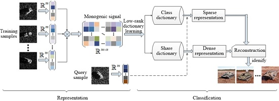
Inspired by the aforementioned works, this paper presents a target recognition strategy, i.e., joint sparse and dense representation of monogenic signal (JMSDR), to solve these problems. To capture the spatial localization and broad spectral information of SAR images, the multi-scale monogenic components of monogenic signal are employed for the production of the monogenic features. Different from directly using the monogenic features to generate low-rank dictionary for spare representation, a class dictionary and a shared dictionary are learned through decomposing the monogenic features. Specifically, the class dictionary focuses on the difference information among each class, while the shared dictionary reflects the common information between different classes. For a vehicle target example, the difference information is used to distinguish different vehicle targets, such as a tank or an armored vehicle, while the common information distinguishes whether the target is a vehicle or an airplane.Moreover, a query sample is jointly represented by the sparse representation of the class dictionary and dense representation of the shared dictionary. Hence, the query sample could be better represented by the variation information of other classes, when the targets are insufficient variations in the specific class of training samples. Additionally, the discriminability of the learned dictionary can be promoted by the low rank constraint. Finally, the decision is made by evaluating the class with the minimal reconstruction error. A block diagram of the proposed strategy is shown in Figure 1.

In the following, Section 2 first introduces the feature representation of SAR image on monogenic signal, and presents the joint sparse and dense representation of monogenic signal strategy. Section 3 evaluate the validity of the proposed strategy on extensive comparative experiments under EOCs. The conclusion is drawn in Section 4.

2. The Proposed Strategy

2.1. The Monogenic Signal

The monogenic signal is a two-dimensional (2-D) analytical signal tool [30]. Generally, a 1-D analytic signal can be represented by Hilbert transform. As the monogenic signal realizes the generalization of Hilbert transform via Riesz transform, the monogenic signal of 2-D signal $f\left(\mathbf{z}\right)$ can be given as

$$f_{\mathcal{M}}\left(\mathbf{z}\right)=f\left(\mathbf{z}\right)-(i,j)·f_{\mathcal{R}}\left(\mathbf{z}\right)$$

(1)

where $f_{\mathcal{R}}\left(\mathbf{z}\right)$ is the Riesz transform of $f\left(\mathbf{z}\right)$.

Practically, the image is a 2-D signal with a finite length. Generally, the log-Gabor filter is applied for pursuing infinite extension of image in spatial domain due to its capability without the disturbance from the limited bandwidth. Then, the 2-D image signal $f\left(\mathbf{z}\right)$ can be expressed as

$$f_L\left(\mathbf{z}\right)=f\left(\mathbf{z}\right)\ast F^{-1}\left(G\left(\omega \right)\right)$$

(2)

where $G\left(\omega \right)$ is the frequency response function of log-Gabor filter. $F^{-1}$ is the inverse Fourier transform. The monogenic signal is rewritten by the Riesz transform

$$f_{\mathcal{M}}\left(\mathbf{z}\right)=f_L\left(\mathbf{z}\right)-(i,j)\left(f_L\left(\mathbf{z}\right)\ast h\left(\mathbf{z}\right)\right)$$

(3)

where $f_{\mathcal{M}}$ is composed of $s=[1,2,\dots ,S]$ scale monogenic feature vectors. The S-scale monogenic feature vector of image signal can be expressed as

$$\mathcal{X}\left(\mathbf{z}\right)=[f_{\mathcal{M}}^1,f_{\mathcal{M}}^2,\dots ,f_{\mathcal{M}}^S]$$

(4)

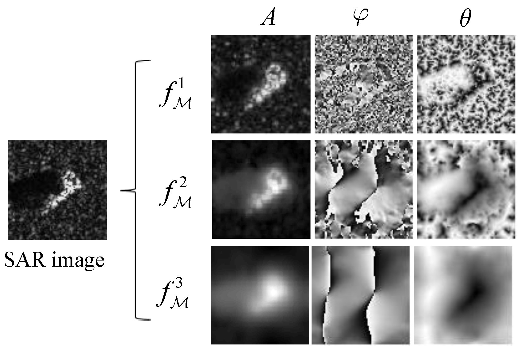
where $f_{\mathcal{M}}^i$ ($i\in s$) is the ith scale monogenic feature vector. It is made up of local amplitude $A_i$, local phase ${\phi }_i$ and local orientation ${\theta }_i$ in order, i.e., $[A_i,{\phi }_i,{\theta }_i]$. Specifically,

$$\begin{array}{c}\hfill A_i=\sqrt{{f_{L,i}}^2\left(\mathbf{z}\right)+{f_{Lx,i}}^2\left(\mathbf{z}\right)+{f_{Ly,i}}^2{\left(\mathbf{z}\right)}^2}\\ \hfill {\phi }_i=-\mathrm{sign}\left(f_{Lx,i}\left(\mathbf{z}\right)\right)arctan2\left(\frac{\sqrt{{f_{Lx,i}}^2\left(\mathbf{z}\right)+{f_{Ly,i}}^2\left(\mathbf{z}\right)}}{f_{L,i}\left(\mathbf{z}\right)}\right)\\ \hfill {\theta }_i=arctan\left(\frac{f_{Ly,i}\left(\mathbf{z}\right)}{f_{Lx,i}\left(\mathbf{z}\right)}\right)\end{array}$$

(5)

where $i\in s=[1,2,\dots ,S]$, s is the scale index. $f_{Lt,i}\left(\mathbf{z}\right)=f_{L,i}\left(\mathbf{z}\right)\ast h_t\left(\mathbf{z}\right),t\in \{x,y\}$. Figure 2 illustrates an example of monogenic components with a SAR image. The image characterized by the monogenic signals in multiple scales could be interpreted as the combination of multiple sub-bands that are from different information spaces. Recently, many methods are proposed to use these synthetic or transformed sub-bands for target detection and recognition [31,32].

2.2. Low-Rank Dictionary Learning

Let $\mathbf{X}=[{\mathbf{X}}_1,{\mathbf{X}}_2,\dots ,{\mathbf{X}}_n]\in {\mathbb{R}}^{m\times n}$ be n training samples, the monogenic feature of training samples generated by Equation (4) is $\mathcal{X}\left(\mathbf{X}\right)=\left[\mathcal{X}\left({\mathbf{X}}_1\right),\mathcal{X}\left({\mathbf{X}}_2\right),\dots ,\mathcal{X}\left({\mathbf{X}}_n\right)\right]$. In [14], the monogenic feature is directly utilized as a dictionary, and then a query sample is sparsely represented and assigned to the class for which the reconstruction error is minimal. However, the signal prespecified dictionary cannot guarantee a valid representation for a query sample when the variations of some classes in training samples are not sufficient. Additionally, it is difficult to perform well when training samples have occlusion and noise corruption.

To overcome these problems, a class dictionary and a shared dictionary are learned to jointly represent query sample through decomposing the monogenic feature. For vehicle target, the class dictionary focuses on the class information in the training sample, for example the vehicle target is a tank or an armored vehicle. The shared dictionary pays more attention to the common information with the vehicle targets provided in the training samples, such as phase and direction. Hence, when the query sample cannot be sufficient represented by the targets from the same class, it can be further linearly represented by the common information provided by the other classes targets in the shared dictionary. Therefore, the monogenic feature $\mathcal{X}\left(\mathbf{X}\right)$ can be decomposed

$$\mathcal{X}\left(\mathbf{X}\right)=\mathsf{\Phi }\mathbf{A}+\mathsf{\Psi }\mathbf{Z}+\mathbf{E}$$

(6)

where $\mathsf{\Phi }$ is the class dictionary, $\mathbf{A}=\{a_{ij},i,j=1\dots n\}$ is a sparse coefficient matrix associated with the class dictionary, $\mathsf{\Psi }$ is the shared dictionary, $\mathbf{Z}$ is a coefficient matrix corresponding with the shared dictionary, and $\mathbf{E}$ is the error matrix. Since the class dictionary only contains the components of specific class, the sparse coefficient should coincide with the class information of sample classes. Hence, the sparse coefficient $a_{ij}\in \mathbf{A}$ meets the following conditions

$$a_{ij}=\left\{\begin{array}{cc}1,\hfill & \mathrm{if}i=j\hfill \\ 0,\hfill & \mathrm{otherwise}\hfill \end{array}\right.$$

(7)

According to the above formula, the sparse coefficient $\mathbf{A}$ is a matrix. Equation (6) can be simplified as follows

$$\mathcal{X}\left(\mathbf{X}\right)=\mathsf{\Phi }+\mathsf{\Psi }\mathbf{Z}+\mathbf{E}$$

(8)

Based on manifold learning theory, the samples from the same class all reside in a low-dimensional subspace [33]. Therefore, the class matrix $\mathsf{\Phi }$ should be approximately low rank. Accordingly, $\mathsf{\Psi }\mathbf{Z}$, $\mathsf{\Psi }$ and $\mathbf{E}$ are also low rank matrices. To make the representation error $\mathbf{E}$ for the query sample as small as possible, the coefficient matrix $\mathbf{Z}$ is reasonably assumed to be not sparse but dense. Hence, the low-rank regularized sparse and dense dictionary learning model based on monogenic features is expressed as

$$\begin{array}{c}\hfill \underset{\varphi ,\mathsf{\Psi },\mathbf{Z},\mathbf{E}}{min}{\parallel \mathsf{\Phi }\parallel }_{\ast }+{\lambda \parallel \mathsf{\Psi }\parallel }_{\ast }+{\gamma \parallel \mathbf{Z}\parallel }_F^2+\tau {\parallel \mathbf{E}\parallel }_1\\ \hfill \mathrm{s}.\mathrm{t}.\mathcal{X}\left(\mathbf{X}\right)=\mathsf{\Phi }+\mathsf{\Psi }\mathbf{Z}+\mathbf{E}\end{array}$$

(9)

where $\lambda ,\gamma$ and $\tau$ are regularization parameter. $\parallel ·\parallel$ represents the nuclear norm that is a convex relaxation of low-rank constrained matrix, and ${\parallel ·\parallel }_F$ is Frobenius norm. Since the objective model in Equation (9) is nonconvex, it is solved by three sub-optimization procedures.

(1) Update the shared dictionary $\mathsf{\Psi }$. The class dictionary $\mathsf{\Phi }$ and dense coefficient matrix $\mathbf{Z}$ are fixed. The optimization problem in Equation (9) is then reduced to

$$\begin{array}{c}\hfill \underset{\mathsf{\Psi },\mathbf{E}}{min}{\parallel \mathsf{\Psi }\parallel }_{\ast }+\eta {\parallel \mathbf{E}\parallel }_1\hfill \\ \hfill \mathrm{s}.\mathrm{t}.\mathcal{X}\left(\mathbf{X}\right)-\mathsf{\Phi }=\mathsf{\Psi }\mathbf{Z}+\mathbf{E}\hfill \end{array}$$

(10)

where $\eta$ is a regularization parameter. The problem in Equation (10) is a classical robust principal component analysis (RPCA) problem [34]. Inexact ALM method [35,36] is utilized to solve this problem. To remedy the issue in solving Equation (10), an auxiliary variable $\mathbf{J}$ is employed to make it separable. Hence, Equation (10) is transformed as

$$\begin{array}{cc}\hfill & \underset{\mathsf{\Psi },\mathbf{J},\mathbf{E}}{min}{\parallel \mathbf{J}\parallel }_{\ast }+\eta {\parallel \mathbf{E}\parallel }_1\hfill \\ \hfill \mathrm{s}.\mathrm{t}.& \mathcal{X}\left(\mathbf{X}\right)-\mathsf{\Phi }=\mathsf{\Psi }\mathbf{Z}+\mathbf{E},\mathsf{\Psi }=\mathbf{J},\mathbf{J}\ge 0\hfill \end{array}$$

(11)

The augmented Lagrangian function of Equation (11) is written as

$$\begin{array}{cc}\hfill {\mathcal{L}}_2=& {\parallel \mathbf{J}\parallel }_{\ast }+\eta {\parallel \mathbf{E}\parallel }_1+tr\left({\mathbf{Y}}_1^T(\mathcal{X}\left(\mathbf{X}\right)-\mathsf{\Phi }-\mathsf{\Psi }-\mathsf{\Psi }\mathbf{Z}-\mathbf{E})\right)+tr\left({\mathbf{Y}}_2^T(\mathsf{\Psi }-\mathbf{J})\right)\hfill \\ & +\frac{\mu }{2}\left({\parallel \mathcal{X}\left(\mathbf{X}\right)-\mathsf{\Phi }-\mathsf{\Psi }\mathbf{Z}-\mathbf{E}\parallel }_F^2+{\parallel \mathsf{\Psi }-\mathbf{J}\parallel }_F^2\right)\hfill \end{array}$$

(12)

where ${\mathbf{Y}}_1$ and ${\mathbf{Y}}_2$ are the Lagrange multipliers, and $\mu >0$ is a penalty parameter. By fixing $\mathsf{\Psi }$ and $\mathbf{E}$, the closed-form solution of $\mathbf{J}$ is

$${\mathbf{J}}^{k+1}=max{\mathcal{D}}_{{\mu }^{-1}}\left({\mathsf{\Psi }}^{k+1}+\frac{1}{\mu }{{\mathbf{Y}}_2}^k\right)$$

(13)

where ${\mathcal{D}}_{\epsilon }\left(r\right)=\mathrm{sgn}\left(r\right)max\left(\right|r|-\epsilon ,0)$. Similarly, for updating $\mathbf{E}$, the closed-form solution can be obtained

$${\mathbf{E}}^{k+1}={\mathcal{D}}_{\eta {\mu }^{-1}}\left(\mathcal{X}\left(\mathbf{X}\right)-\mathsf{\Phi }-{\mathsf{\Psi }}^{k+1}\mathbf{Z}+\frac{1}{\mu }{\mathbf{Y}}_1^k\right)$$

(14)

Fixing $\mathbf{J}$ and $\mathbf{E}$, the closed-form solution for updating $\mathsf{\Psi }$ can be acquired

$${\mathsf{\Psi }}^{k+1}=\left[\left(\mathcal{X}\left(\mathbf{X}\right)-\mathsf{\Phi }-{\mathbf{E}}^k\right){\left({\mathbf{Z}}^k\right)}^T+\left({\left({\mathbf{Z}}^k\right)}^T{\mathbf{Y}}_1^k-\frac{1}{\mu }{\mathbf{Y}}_2^k\right)+{\mathbf{J}}^{k+1}\right]{\left(\mathbf{I}+{\mathbf{Z}}^k{\left({\mathbf{Z}}^k\right)}^T\right)}^{-1}$$

(15)

According to ${\mathbf{Y}}_1^{k+1}={\mathbf{Y}}_1^k+\mu (\mathcal{X}\left(\mathbf{X}\right)-\mathsf{\Phi }-\mathsf{\Psi }\mathbf{Z}-\mathbf{E})$ and ${\mathbf{Y}}_2^{k+1}={\mathbf{Y}}_2^k+\mu (\mathsf{\Psi }-\mathbf{J})$, the Lagrange multipliers ${\mathbf{Y}}_1$ and ${\mathbf{Y}}_2$ are updated. When the termination condition $\parallel \mathcal{X}\left(\mathbf{X}\right)-\mathsf{\Phi }-{\mathsf{\Psi }}^{k+1}\mathbf{Z}-{\mathbf{E}}^{k+1}{\parallel }_F^2<\epsilon$ and $|{\mathsf{\Psi }}^{k+1}-{\mathbf{J}}^{k+1}{|}_F^2<\epsilon$ is met, $\mathsf{\Psi }={\mathsf{\Psi }}^{k+1}$ is the solution of the optimization problem in Equation (12).

(2) Update dense coefficient matrix $\mathbf{Z}$. The class dictionary $\mathsf{\Phi }$ and the shared dictionary $\mathsf{\Psi }$ are fixed. The optimization problem in Equation (9) can be replaced as:

$$\begin{array}{c}\hfill \underset{\mathbf{Z},\mathbf{E}}{min}{\gamma \parallel \mathbf{Z}\parallel }_1+\tau {\parallel \mathbf{E}\parallel }_1\hfill \\ \hfill \mathrm{s}.\mathrm{t}.\mathcal{X}\left(\mathbf{X}\right)-\mathsf{\Phi }=\mathsf{\Psi }\mathbf{Z}+\mathbf{E}\hfill \end{array}$$

(16)

Similarly, the problem can also be solved by Inexact ALM method, whose augmented Lagrangian function is expressed as

$$\begin{array}{cc}\hfill {\mathcal{L}}_3=& {\gamma \parallel \mathbf{Z}\parallel }_F^2+\tau {\parallel \mathbf{E}\parallel }_1+tr\left({\mathbf{Y}}^T(\mathcal{X}\left(\mathbf{X}\right)-\mathsf{\Phi }-\mathsf{\Psi }\mathbf{Z}-\mathbf{E})\right)\hfill \\ & +\frac{\mu }{2}\left({\parallel \mathcal{X}\left(\mathbf{X}\right)-\mathsf{\Phi }-\mathsf{\Psi }\mathbf{Z}-\mathbf{E}\parallel }_F^2\right)\hfill \end{array}$$

(17)

The solution of the optimization problem in Equation (17) procedure can be summarized in Algorithm 1.

Algorithm 1 The procedure of solving the optimization problem in Equation (17).

Input: the monogenic features of training sample matrix $\mathcal{X}\left(\mathbf{X}\right)$  class dictionary $\mathsf{\Psi }$, shared dictionary $\mathsf{\Phi }$  parameters $\gamma$ and $\tau$, and threshold $\epsilon$. Output: dense coefficient matrix $\mathbf{Z}$.  Initialization:  $\mathbf{E}=\mathbf{Y}=0,\mu ={10}^{-6},{\mu }_{m}ax={10}^6,\rho =2,ϵ={10}^{-6}$.  While not converged $(k=0,1,\dots )$ do  Update $\mathbf{Z}$ by fixing $\mathbf{E}$ ${\mathbf{Z}}^{k+1}=\mu {\left(2\gamma \mathbf{I}+\mu {\mathsf{\Psi }}^T\mathsf{\Psi }\right)}^{-1}{\mathsf{\Psi }}^T\left(\mathcal{X}\left(\mathbf{X}\right)-\mathsf{\Phi }-{\mathbf{E}}^k-\frac{1}{\mu }{\mathbf{Y}}^k\right)$  Update $\mathbf{E}$ by fixing $\mathbf{Z}$ ${\mathbf{E}}^{k+1}={\mathcal{D}}_{\tau {\mu }^{-1}}\left(\mathcal{X}\left(\mathbf{X}\right)-\mathsf{\Phi }-\mathsf{\Psi }{\mathbf{Z}}^{k+1}+\frac{1}{\mu }{\mathbf{Y}}^k\right)$  Update Lagrange multiplier $\mathbf{Y}$ ${\mathbf{Y}}^{k+1}={\mathbf{Y}}^k+\mu (\mathcal{X}\left(\mathbf{X}\right)-\mathsf{\Phi }-\mathsf{\Psi }{\mathbf{Z}}^{k+1}-{\mathbf{E}}^{k+1})$  Update $\mu$ through ${\mu }^{k+1}=min({\mu }_{max},\rho {\mu }^k)$  Check convergence: if $|\mathcal{X}\left(\mathbf{X}\right)-\mathsf{\Phi }-\mathsf{\Psi }{\mathbf{Z}}^{k+1}-{\mathbf{E}}^{k+1}|<\epsilon$, then stop.  End

(3) Update the class dictionary $\mathsf{\Phi }$. The shared dictionary $\mathsf{\Psi }$ and dense coefficient matrix $\mathbf{Z}$ are fixed. The optimization problem in Equation (9) is simplified as

$$\begin{array}{c}\hfill \underset{\mathsf{\Phi },\mathbf{E}}{min}{\parallel \mathsf{\Phi }\parallel }_{\ast }+\tau {\parallel \mathbf{E}\parallel }_1\hfill \\ \hfill \mathrm{s}.\mathrm{t}.\mathcal{X}\left(\mathbf{X}\right)-\mathsf{\Psi }\mathbf{Z}=\mathsf{\Phi }+\mathbf{E}\hfill \end{array}$$

(18)

where $\eta$ is a regularization parameter. The above equation is a classical robust principal component analysis model, which can be transformed into the problem of minimizing Lagrangian function

$$\begin{array}{cc}\hfill {\mathcal{L}}_1=& {\parallel \mathsf{\Phi }\parallel }_{\ast }+\tau {\parallel \mathbf{E}\parallel }_1+tr\left({\mathbf{Y}}^T(\mathcal{X}\left(\mathbf{X}\right)-\mathsf{\Psi }\mathbf{Z}-\mathsf{\Phi }-\mathbf{E})\right)\hfill \\ & +\frac{\mu }{2}\left({\parallel \mathcal{X}\left(\mathbf{X}\right)-\mathsf{\Psi }\mathbf{Z}-\mathsf{\Phi }-\mathbf{E}\parallel }_F^2\right)\hfill \end{array}$$

(19)

Equation (19) is an unconstrained problem, thus this problem can be solved by repeatedly setting $\begin{array}{c}\hfill {\mathcal{L}}_1\left({\mathsf{\Phi }}^k,{\mathbf{E}}^k\right)=arg\underset{\mathsf{\Phi },\mathbf{E}}{min}{\mathcal{L}}_1\left(\mathsf{\Phi },\mathbf{E},{\mathbf{Y}}^k\right)\end{array}$, separately updating variables, and then updating the Lagrange multiplier ${\mathbf{Y}}^{\mathbf{k}+\mathbf{1}}$. Specifically, the update optimization process is as follows

$$\begin{array}{c}{\mathsf{\Phi }}^{k+1}={\mathcal{D}}_{{\mu }^{-1}}\left(\mathcal{X}\left(\mathbf{X}\right)-\mathsf{\Psi }\mathbf{Z}-{\mathbf{E}}^k+{\mathbf{Y}}^k/\mu \right)\hfill \\ {\mathbf{E}}^{k+1}={\mathcal{D}}_{\tau {\mu }^{-1}}\left(\mathcal{X}\left(\mathbf{X}\right)-\mathsf{\Psi }\mathbf{Z}-{\mathsf{\Phi }}^{k+1}+{\mathbf{Y}}^k/\mu \right)\hfill \\ {\mathbf{Y}}^{k+1}={\mathbf{Y}}^k+\mu \left(\mathcal{X}\left(\mathbf{X}\right)-\mathsf{\Psi }\mathbf{Z}-{\mathsf{\Phi }}^{k+1}-{\mathbf{E}}^{k+1}\right)\hfill \end{array}$$

(20)

When the termination condition $\parallel \mathcal{X}\left(\mathbf{X}\right)-\mathsf{\Psi }\mathbf{Z}-{\mathsf{\Phi }}^{k+1}-{\mathbf{E}}^{k+1}{\parallel }_F^2<\epsilon$ is met, $\mathsf{\Phi }={\mathsf{\Phi }}^{k+1}$ is the solution of the optimization problem in Equation (19).

By sequentially solving Equations (10), (16) and (18), the shared dictionary and the class dictionary of monogenic features are acquired. The shared dictionary $\mathsf{\Phi }$ contains more common information of the target, and the class dictionary $\mathsf{\Psi }$ contains more category information. More importantly, the dense coefficient matrix $\mathbf{Z}$ improves the ability of the dictionary to represent query samples rather than directly using the training sample themselves as a dictionary. Hence, the problems about insufficient variations of training samples, occlusion and noise corruption can be alleviated. The flow diagram of low-rank dictionary learning is shown in Figure 3.

2.3. Implementation of Target Recognition

The low-rank dictionary learning is presented in the previous section. Then, target classification with the learned dictionaries including the shared dictionary and the class dictionary is implemented.

Given the training samples and relevant class labels from C classes, $\mathbf{X}=\left[{\mathbf{x}}_1,{\mathbf{x}}_2,\dots ,{\mathbf{x}}_n\right]\in {\mathbb{R}}^{m\times n}$. We first compute the augmented monogenic features of training samples by Equation (4)

$$\mathcal{X}\left(\mathbf{X}\right)=\left[\mathcal{X}\left({\mathbf{x}}_1\right),\mathcal{X}\left({\mathbf{x}}_2\right),\dots ,\mathcal{X}\left({\mathbf{x}}_n\right)\right]$$

(21)

Those features are then used to produce a shared dictionary and a class dictionary. Specifically, the two learned dictionary can be obtained by solving the low-rank dictionary learning model in Equation (9). Given a query sample $\mathbf{y}$, the monogenic feature of the query sample can be represented by $\chi \left(\mathbf{y}\right)$. The query sample can be encoded by the shared dictionary $\mathsf{\Phi }$ and the class dictionary $\mathsf{\Psi }$ as a linear combination of themselves.

$$\mathcal{X}\left(\mathbf{y}\right)=\mathsf{\Phi }\mathit{\alpha }+\mathsf{\Psi }\mathbf{z}+\mathbf{e}$$

(22)

where $\alpha$ is a sparse coefficient related to the class dictionary $\mathsf{\Psi }$ and $\mathbf{z}$ is a dense coefficient corresponding with the shared dictionary $\mathsf{\Phi }$. Generally, the method for obtaining the sparse solution is to constrain the feasible set by sparse constraint. For example, ${\ell }_1—$norm minimization of the sparse representation $\alpha$ is applied. In addition, we use ${\ell }_2—$norm to realize the dense representation $\mathbf{z}$. To make it robust to occlusion and noise corruption, the error $\mathbf{e}$ uses ${\ell }_1—$norm minimization. Therefore, the joint sparse and dense representation of query sample can be described as follows:

$$\begin{array}{c}\hfill \underset{\mathit{\alpha },\mathbf{z},\mathbf{e}}{min}{\parallel \mathit{\alpha }\parallel }_1+{\kappa \parallel \mathbf{z}\parallel }_2^2+\varphi {\parallel \mathbf{e}\parallel }_1\\ \hfill \mathrm{s}.\mathrm{t}.\mathcal{X}\left(\mathbf{y}\right)=\mathsf{\Phi }\mathit{\alpha }+\mathsf{\Psi }\mathbf{z}+\mathbf{e}\end{array}$$

(23)

where $\kappa$ and $\varphi$ are regularization parameters. To solving the problem in Equation (23), we also adopt the inexact ALM method. Thus, the optimization problem can be transferred into an augmented Lagrangian function.

$$\begin{array}{cc}\hfill \mathcal{J}=& {\parallel \mathit{\alpha }\parallel }_1+{\kappa \parallel \mathbf{z}\parallel }_2^2+{\varphi \parallel \mathbf{e}\parallel }_1+\frac{\psi }{2}{\parallel \mathcal{X}\left(\mathbf{y}\right)-\mathsf{\Phi }\mathit{\alpha }-\mathsf{\Psi }\mathbf{z}-\mathbf{e}\parallel }_2^2\hfill \\ & +{\mathbf{p}}^T(\mathcal{X}\left(\mathbf{y}\right)-\mathsf{\Phi }\mathit{\alpha }-\mathsf{\Psi }\mathbf{z}-\mathbf{e})\hfill \end{array}$$

(24)

where $\varphi >0$ is a penalty parameter and $\mathbf{p}$ is the Lagrange multiplier.

By minimizing the augmented Lagrangian function, the variables are updated alternately while keeping other variables unchanged. The iteration stops when it meets the convergence condition.

Since the class dictionary includes the class information of samples, the sparse representation part coincides with the class-label. Thus, the decision is made by calculating the class which has the minimal reconstruction error.

$$\begin{array}{c}\hfill \underset{k\in 1,2,\dots ,C}{min}{∥\mathsf{\Phi }\mathit{\alpha }-{\delta }_k\left(\mathsf{\Phi }\right)\mathit{a}∥}_2^2\end{array}$$

(25)

Algorithm 2 summarizes the proposed strategy JMSDR for SAR target recognition.

Algorithm 2 Target recognition via joint sparse and dense representation of monogenic signal (JMSDR).

Input: training sample $\mathbf{X}=\left[{\mathbf{x}}_1,{\mathbf{x}}_2,\dots ,{\mathbf{x}}_n\right]\in {\mathbb{R}}^{m\times n}$ and query sample $\mathbf{y}$. Output: class label of $\mathbf{y}$.  Step 1: Compute multi-scale monogenic features of training samples ${\left\{\mathcal{X}\left({\mathbf{x}}_i\right)\right\}}_{i=1}^n$.  Step 2: Compute multi-scale monogenic features of query sample $\mathcal{X}\left(\mathbf{y}\right)$.  Step 3: Learn a shared dictionary $\mathsf{\Phi }$ and a class dictionary $\mathsf{\Psi }$ with Equation (9).  Step 4: Compute the sparse representation and the dense representation of query sample over the learned dictionary, as shown in Equation (23).  Step 5: Predict the identity by seeking the minimal reconstruction error, as defined in Equation (25).

3. Experiments and Discussion

This section evaluates the performance of the proposed strategy on MSTAR database. All target images chips cover all $0^{\circ }$–${359}^{\circ }$ aspect angles at a range of depression angles ${15}^{\circ }$ and ${17}^{\circ }$. We cropped 64 × 64 pixels for all samples from the center of the original 128 × 128 pixels images to reduce the influence of the background. Series of experiments were performed under extended operating conditions, including configuration variation, version variation, partial occlusion and noise corruption. The proposed strategy JMSDR was compared with several studied methods in terms of recognition performance: MSRC [14], ESRC [22], FDDL [37], LRSDL [38], SSRC [23], and all-convolutional network (A-ConvNets) [39]. The scale parameters for monogenic signal was set to $S=3$. The parameters of the proposed strategy JMSDR were experimentally set as $\kappa =\varphi =10$.

3.1. Preliminary Verification

The performance of the proposed strategy was assessed firstly on the four classes targets, i.e., BMP2, BTR60, T72 and T62. The images acquired with ${17}^{\circ }$ and ${15}^{\circ }$ of depression angle were set as training and testing, respectively. The type and number of samples, as well as the series number of configuration, are all listed in

Table 1. The training and testing samples in the experiments.

Type	Depr.	BMP2	BTR60	T72	T62	Total
Training	17°	233(SN_9563)	256	233(SN_132)	299	1020
Testing	15°	195(SN_9563) 196(SN_9566) 196(SN_C21)	195	196(SN_132) 195(SN_812) 195(SN_S7)	273	1637

. The detail of configuration is explained in Section 3.2. The examples of four classes targets are shown in Figure 4.

The recognition performance across different methods is listed in

Table 2. The recognition accuracy on four-class target by different methods.

Method	MSRC	FDDL	ESRC	LRSDL	SSRC	JMSDR
Accuracy	0.9096	0.8931	0.9198	0.9023	0.9267	0.9318

. The recognition accuracy of the proposed strategy JMSDR is higher than that of MSRC because the discriminative ability can be promoted by learning dictionary. Compared to 0.8931 for FDDL, 0.9198 for ESRC, 0.9023 for LRSDL, and 0.9267 for SSRC, the recognition results show that the JMSDR outperforms these dictionary learning methods, demonstrating that the jointed sparse and dense representation can represent the samples more accurately. The experimental result reveals that joint sparse and dense representation of multi-scale monogenic components is an effective way to describe targets for classification.

3.2. Results on 10-Class

To comprehensively assess the performance of the proposed strategy, we firstly performed the experiment on 10-class target recognition. The training samples and the test samples were collected at ${17}^{\circ }$ and ${15}^{\circ }$ depression angles, respectively. The types of targets ( BMP2 and T72) in test samples were not covered by the training samples. The type and numbers of training and testing samples can be found in

Table 3. The number of images for ten class targets.

Depr.	BMP2	BTR70	T72	2S1	BRDM	BTR60	D7	T62	ZIL	ZSU
17°	233(SN_9563)	233	233(SN_132)	299	298	256	299	299	299	299
15°	196(SN_9566) 196(SN_c21)	196	195(SN_812) 191(SN_s7)	274	274	195	273	273	274	274

.

In

Table 4. The recognition accuracy on 10-class target by different methods.

Method	MSRC	FDDL	ESRC	LRSDL	SSRC	A-ConvNets	JMSDR
Accuracy	0.9279	0.8868	0.9317	0.9168	0.9420	0.9552	0.9356

, we compare the recognition results of MSRC, FDDL, ESRC, LRSDL, SSRC, A-ConvNets and the proposed strategy for 10-class targets. The best results come from A-ConvNets, which is 1.96% better than JMSDR method. Specifically, JMSDR attains a high recognition accuracy of 0.9356. It is fairly comparable to the SSRC, and outperforms the MSRC, FDDL, ESRC and LRSDL methods by margins of 0.77%, 4.88%, 0.39% and 2.62%, respectively.

3.3. Results on Configuration Variance

Configuration variance is inevitable for SAR target recognition, as the targets have physical differences and structure modifications. To evaluate the reliability and stability of JMSDR under the configuration variance EOC, the four-class problem (denoted by configuration variance EOC-1) with training and testing samples chosen from BMP2, BTR60, T72 and T62, was firstly considered. The standards of BMP2 and T72 were used for training, while the other variants were employed for testing, as described in Table 1.

Table 5. The recognition accuracy of different methods under configuration variance EOC-1.

Method	MSRC	FDDL	ESRC	LRSDL	SSRC	A-ConvNets	JMSDR
Accuracy	0.8852	0.8812	0.8967	0.8949	0.9109	0.9436	0.9213

shows the performance comparison between the proposed strategy JMSDR and the basic methods. Except for a marginal difference compared with A-ConvNets, the proposed strategy JMSDR achieves a better recognition performance than the other methods. Specifically, the recognition accuracies for MSRC, FDDL, ESRC, and LRSDL are all below 0.9.

Table 6. The training and testing samples in the configuration variance EOC-1 experiments.

Type	BMP2	BTR60	T72	T62	Accuracy
BMP2	358	4	28	2	0.9132
BTR60	2	180	2	11	0.9230
T72	0	1	339	46	0.8782
T62	0	0	2	271	0.9926
Average					0.9213

gives the confusion matrix of JMSDR. In Table 6, we can see that the performance for BTR60 and T62 are satisfactory, while BMP2 and T72 are more like to be misclassified. This is because BMP2 and T72 in the training and testing sets employ different types of targets. Compared to the other methods, JMSDR could achieves a better performance when the configuration variants of targets in training samples are insufficient.

Then, we considered another four-class configuration variance problem (denoted by configuration variance EOC-2). Specifically, the training samples were chosen from BMP2, BRDM, BTR70 and T72, and the test set comprised two variants of BMP2 and five variants of T-72. The detailed information is listed in

Table 7. The training and testing samples in the configuration variance EOC-2 experiments.

Type	Depr.	BMP2	BRDM	BTR70	T72	Total
Training	17°	233(SN_C21)	298(SN_E71)	233(SN_C71)	232(SN_132)	996
Testing	15°	428(SN_9563)	0	0	426(SN_812)	3568
					573(SN_A04)
		428(SN_9566)			573(SN_A05)
					573(SN_A07)
					573(SN_A10)

. Both configurations were different between the training images and testing images. Figure 5 shows an example of optical and SAR images for several T72 configuration variants.

Table 8. The recognition performances of different methods under configuration variance EOC-2.

Method	MSRC	FDDL	ESRC	LRSDL	SSRC	A-ConvNets	JMSDR
Accuracy	0.9148	0.9176	0.9403	0.9190	0.9279	0.9770	0.9543

shows the overall recognition accuracies of MSRC, FDDL, ESRC, LRSDL, SSRC and the proposed strategy JMSDR. The confusion matrix of the recognition results for each method is shown in Figure 6. In each subfigure, the row and column corresponding to the same class describe the number of correct classifications. From the confusion matrix, it can be seen that BMP2 is more easily misclassified than T72. This is because that targets of T72 have more common information in the testing samples and training samples. Therefore, compared to BMP2, T72 is better represented by the training samples. Table 8 shows that the MSRC gets the worst recognition result, which reveals that the prespecified dictionary cannot deal well with the configuration variance. The overall recognition accuracy of JMSDR is 0.9543, which is better than MSRC (0.9148), FDDL (0.9176), ESRC (0.9403), LRSDL (0.9190), and SSRC (0.9279) and is fairly comparable with A-ConvNets. The experimental results confirm the validity of the joint sparse and dense representation, which could deal with the configuration variance even under multiple structure variants.

3.4. Results on Version Variance

The version variant refers to targets of the same class but built with different blueprints [40]. In practical applications, the training set usually consists of different versions of the target. Therefore, the following experiment evaluated the recognition performance of the proposed strategy JMSDR under the version variant EOC. In the MSTAR public dataset, T72 has multiple versions. The official recommendation is that the version SN_132 of T72 is set as the training samples, while the other versions of T72 including SN_S7, SN_A32, SN_A62, SN_A63 and SN_A64 are set as testing samples. In addition, BMP2, BRDM2 and BTR70 were included in the training dataset as the interference items for target recognition. Since the versions of targets in training samples were insufficient, the difficulty of target recognition was increased. All training samples were collected at a ${17}^{\circ }$ depression angle, while the testing samples were collected at both ${15}^{\circ }$ and ${17}^{\circ }$ depression angles.

Table 9. The training and testing samples in the version variance EOC experiments.

Type	Depr.	BMP2	BRDM	BTR70	T72	Total
Training	17°	233(SN_C21)	298(SN_E71)	233(SN_C71)	232(SN_132)	996
Testing	15° and 17°	0	0	0	419(SN_S7) 572(SN_A32) 573(SN_A62) 573(SN_A63) 573(SN_A64)	2710

list the detail information on the training and testing samples. An example of the optical and SAR images of the target under T72 version variants is illustrated in Figure 7.

Figure 8 shows both overall recognition rates and confusion matrices for MSRC, FDDL, ESRC, LRSDL, SSRC, A-ConvNets and the proposed strategy JMSDR under version variants EOC. Specifically, each row represents the number of targets that are categorized into each class for a particular version of the T72. Figure 8 shows that the recognition accuracy of MSRC is lowest. It reveals that only the sparse representation of monogenic components cannot sufficiently reconstruct the query sample when the information included in training sample is not enough. Compared to MSRC, the performances of FDDL, ESRC, LRSDL, SSRC and A-ConvNets are significantly better. In contrast, the JMSDR represents the query sample more accurately because it learns a common dictionary and a shared dictionary. The performance of JMSDR is 0.9967, which is 1.04%, 4.35%, 3.1%, 2.59%, and 0.96% higher than 0.9863 for FDDL, 0.9535 for ESRC, 0.9657 for LRSDL, 0.9708 for SSRC, and 0.9871 for A-ConvNets, respectively. The experimental results indicate that JMSDR can effectively deal with the SAR target recognition task with version variants.

3.5. Results on Noise Corruption

Real SAR images usually contain noises due to the inherent imaging mechanism. We added random noise to the four-class targets, which were used for conducting the experiment (see Table 1). Specifically, a percentage of pixels from original images was randomly chosen and replaced with independent and identically distributed samples within the image pixel values, which is used in several relevant studies [3,17]. However, the difference is that we randomly corrupted 60% of training samples and testing samples, not all the test samples. In comparison, our experimental setup is more demanding.

Some examples of noise corruption with different noise levels are shown in Figure 9. The percentage of corrupted levels was varied from 10% to 50%. The graph in Figure 10 shows the recognition performance of JMSDR and its four competitors. The proposed strategy outperforms others for all levels of noise corruption. For up to 30% noise corruption, JMSDR correctly identifies over 80% of test samples. Even at 40% corruption, the recognition accuracy of JMSDR is about 10% higher than that of MSRC, FDDL and LRSDL. The results validate that JMSDR is robust towards noise corruption.

3.6. Results on Partial Occlusion

The target could be partially occluded by different obstacles under changing environmental conditions, such as trees or manmade buildings. Hence, it is necessary to evaluate the performance of target recognition on partial occlusion. According to the occlusion method in [41], the levels of occlusion from 0% to 60% were simulated, by replacing target region of each SAR image with the background intensities from eight different directions. Figure 11 shows the original SAR images and the partial occluded SAR images at 25% level from four different directions. In our experiments, we corrupted 60% of training samples and testing samples and their occlusion directions were different, which further increased the difficulty of target recognition.

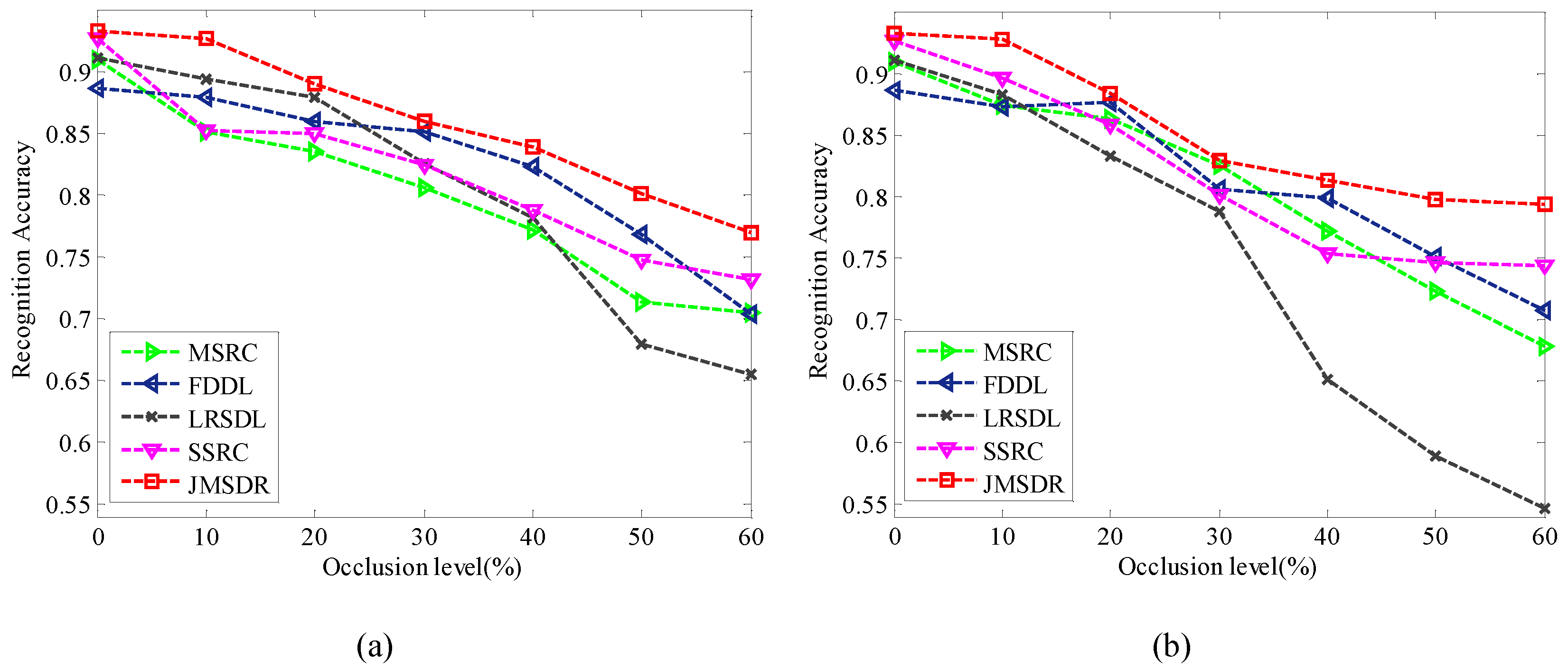
The recognition results are shown in Figure 12. The occlusion directions for training samples and testing samples are Directions 1 and 3 in Figure 12a, respectively. In Figure 12b, the occlusion directions are employed at Direction 1 for training samples and Direction 5 for testing samples. Obviously, the performance of JMSDR is significantly better than the studied methods at all levels of occlusion. When the percentage of occlusion increases, the recognition rates of LRSDL and FDDL quickly drop, while the performance of JMSDR is relatively stable. This can be attributed to the dense representation based on the shared dictionary, as the query sample is represented by more samples which have common information. The results fully demonstrate the advantage of shared dictionary. In addition, the results prove that the proposed strategy could deal with partial occlusion.

4. Conclusions

To handle the extended operation conditions of SAR target recognition, a new strategy is proposed via joint sparse and dense representation of monogenic signal. Unlike the monogenic features of training samples that are directly utilized to generate dictionary for spare representation, a class dictionary and a shared dictionary are learned through decomposing the monogenic features. The combination of the sparse representation of the class dictionary and the dense representation of the shared dictionary provides a better representation of the query sample. Hence, the query sample can better coincide with the right class. According to the results of extensive comparative experiments, some conclusions can be obtained. (1) Compared withthe prespecified dictionary, the learned dictionary, including class dictionary and the shared dictionary, promotes the discriminative ability. (2) Joint sparse representation of class dictionary and dense representation of shared dictionary improves the recognition accuracy. (3) The proposed strategy could deal with various target variants, including configuration variants and version variants, especially for the insufficient variants in training samples. (4) Although there is a large amount of noise corruption and partial occlusion in samples, the proposed strategy still achieved a better recognition results, consistently exceeding the competitors.

References

- Quan, S.; Xiang, D.X.B.K.G. Derivation of the Orientation Parameters in Built-up Areas: With Application to Model-based Decomposition. IEEE Trans. Geosci. Remote Sens. 2016, 56, 337–341. [Google Scholar] [CrossRef]
- Quan, S.; Xiong, B.; Zhang, S.; Yu, M.; Kuang, G. Adaptive and fast prescreening for SAR ATR via change detection technique. IEEE Geosci. Remote Sens. Lett. 2018, 12, 4714–4730. [Google Scholar] [CrossRef]
- Dong, G.; Kuang, G.; Wang, N.; Wang, W. Classification via sparse representation of steerable wavelet frames on grassmann manifold: Application to target recognition in SAR image. IEEE Trans. Image Proc. 2017, 26, 2892–2904. [Google Scholar] [CrossRef] [PubMed]
- Song, S.; Xu, B.; Yang, J. SAR Target Recognition via Supervised Discriminative Dictionary Learning and Sparse Representation of the SAR-HOG Feature. Remote Sens. 2016, 8, 683. [Google Scholar] [CrossRef]
- Osullivan, J.A.; Devore, M.D.; Kedia, V.S.; Miller, M.I. SAR ATR performance using a conditionally Gaussian model. IEEE Trans. Aerosp. Electron. Syst. 2001, 37, 91–108. [Google Scholar] [CrossRef]
- Mossing, J.C.; Ross, T.D. An Evaluation of SAR ATR Algorithm Performance Sensitivity to MSTAR Extended Operating Conditions. Proc. SPIE 1998, 3370, 554–565. [Google Scholar]
- Umamahesh, S.; Vishal, M. SAR automatic target recognition using discriminative graphical modals. IEEE Trans. Aerosp. Electron. Syst. 2014, 50, 591–606. [Google Scholar]
- Novak, L.M.; Owirka, G.J.; Netishen, C.M. Performance of a high-resolution Polarimetric SAR Automatic Target Recognition System. Linc. Lab. J. 1993, 6, 11–24. [Google Scholar]
- Huang, X.Y.; Qiao, H.; Zhang, B. SAR target configuration recognition using tensor global and local discriminant embedding. IEEE Geosc. Remote Sens. Lett. 2016, 13, 222–226. [Google Scholar] [CrossRef]
- Yu, M.T.; Zhao, L.J.; Zhao, S.Q.; Xiong, B.L.; Kuang, G.Y. SAR target reconition using parametric supervised t-stochastic neighbor embedding. Remote Sens. Lett. 2017, 8, 849–858. [Google Scholar] [CrossRef]
- Yu, M.; Dong, G.; Fan, H.; Kuang, G. SAR Target Recognition via Local Sparse Representation of Multi-Manifold Regularized Low-Rank Approximation. Remote Sens. 2018, 10, 211. [Google Scholar]
- Ding, B.Y.; Wen, G.J.; Huang, X.H.; Ma, C.H.; Yang, X.L. Data augmentation by multilevel reconstruction using attributed scattering center for SAR target recognition. IEEE Geosc. Remote Sens. Lett. 2017, 14, 979–983. [Google Scholar] [CrossRef]
- Zhou, J.X.; Shi, Z.G.; Cheng, X.; Fu, Q. Automatic target recognition of SAR images based on global scattering center model. IEEE Trans. Geosc. Remote Sens. 2011, 49, 3713–3729. [Google Scholar]
- Dong, G.; Wang, N.; Kuang, G. Sparse representation of monogenic signal: With application to target recognition in SAR images. IEEE Signal Proc. Lett. 2014, 21, 952–956. [Google Scholar]
- Dong, G.; Kuang, G.; Wang, N.; Zhao, L.; Lu, J. SAR target recognition via joint sparse representation of monogenic signal. IEEE J. Sel. Top. Appl. Earth Obs. Remote Sens. 2015, 8, 3316–3328. [Google Scholar] [CrossRef]
- Zhou, Z.; Wang, M.; Cao, Z.; Pi, Y. SAR Image Recognition with Monogenic Scale Selection-Based Weighted Multi-task Joint Sparse Representation. Remote Sens. 2018, 10, 504. [Google Scholar] [CrossRef]
- Zhou, Y.; Chen, Y.; Cao, R.; Feng, J. SAR Target Recognition via Joint Sparse Representation of Monogenic Components with 2D Cannonical Correlation Analysis. IEEE ACCESS 2019, 7, 25815–25826. [Google Scholar]
- Ramirez, I.; Sprechmann, P.; Sapiro, G. Classification and clustering via dictionary learning with structured incoherence and shared features. In Proceedings of the 2010 IEEE Computer Society Conference on Computer Vision and Pattern Recognition, San Francisco, CA, USA, 13–18 June 2010; pp. 3501–3508. [Google Scholar]
- Mairal, J.; Bach, F.; Ponce, J.; Sapiro, G. Online Learning for Matrix Factorization and Sparse Coding. J. Mach. Learn. Res. 2010, 11, 19–60. [Google Scholar]
- Jiang, Z.; Lin, Z.; Davis, L.S. Label Consistent K-SVD: Learning a Discriminative Dictionary for Recognition. IEEE Trans. Pattern Anal. Mach. Intell. 2013, 35, 2651–2664. [Google Scholar] [CrossRef]
- Dong, G.; Wang, N.; Kuang, G.; Qiu, H. Sparsity and Low-Rank Dictionary Learning for Sparse Representation of Monogenic Signal. IEEE J. Sel. Top. Appl. Earth Obs. Remote Sens. 2018, 11, 141–153. [Google Scholar] [CrossRef]
- Deng, W.; Hu, J.; Guo, J. Extended SRC: Undersampled Face Recognition via Intraclass Variant Dictionary. IEEE Trans. Pattern Anal. Mach. Intell. 2012, 34, 1864–1870. [Google Scholar] [CrossRef] [PubMed]
- Deng, W.; Hu, J.; Guo, J. In Defense of Sparsity Based Face Recognition. In Proceedings of the 2013 IEEE Conference on Computer Vision and Pattern Recognition, Portland, OR, USA, 23–28 June 2013. [Google Scholar]
- Jiang, X.; Lai, J. Sparse and Dense Hybrid Representation via Dictionary Decomposition for Face Recognition. IEEE Trans. Pattern Anal. Mach. Intell. 2015, 37, 1067–1079. [Google Scholar] [CrossRef] [PubMed]
- Li, M.; Guo, Y.; Li, M.; Luo, G.; Kong, X. Coupled Dictionary Learning for Target Recognition in SAR Images. IEEE Geosci. Remote Sens. Lett. 2017, 14, 791–795. [Google Scholar] [CrossRef]
- Otazo, R.; Candes, E.J.; Sodickson, D.K. Low rank plus sparse matrix decomposition for accelerated dynamic MRI with separation of background and dynamic components. Magn. Reson. Med. 2015, 73, 1125–1136. [Google Scholar] [CrossRef]
- Chen, C.F.; Wei, C.P.; Wang, Y.C.F. Low-rank matrix recovery with structural incoherence for robust face recognition. In Proceedings of the 2013 IEEE Conference on Computer Vision and Pattern Recognition, Portland, OR, USA, 23–28 June 2013. [Google Scholar]
- Biondi, F. Low rank plus sparse decomposition of synthetic aperture radar data for maritime surveillance. In Proceedings of the 2016 4th International Workshop on Compressed Sensing Theory and its Applications to Radar, Sonar and Remote Sensing (CoSeRa), Aachen, Germany, 19–22 September 2016. [Google Scholar]
- Leibovich, M.; Papanicolaou, G.; Tsogka, C. Low rank plus sparse decomposition of synthetic aperture radar data for target imaging and tracking. arXiv 2019, arXiv:1906.02311. [Google Scholar]
- Felsberg, M.; Duits, R.; Florack, L. The Monogenic Scale Space on a Rectangular Domain and its Features. Int. J. Comput. Vis. 2005, 64, 187–201. [Google Scholar] [CrossRef]
- Xia, C.; Li, X.; Zhao, L. Infrared Small Target Detection via Modified Random Walks. Remote Sens. 2018, 10, 2004. [Google Scholar] [CrossRef]
- Dao, M.; Kwan, C.; Bernabe, S.J.; Plaza, A.; Koperski, K. A Joint Sparsity Approach to Soil Detection Using Expanded Bands of WV-2 Images. IEEE Geosc. Remote Sens. Lett. 2019. [Google Scholar] [CrossRef]
- Roweis, S.T.; Saul, L.K. Nonlinear dimensionality reduction by locally linear embedding. Science 2000, 290, 2323–2326. [Google Scholar] [CrossRef]
- Candes, E.J.; Li, X.; Ma, Y.; Wright, J. Robust principal component analysis. J. ACM 2011, 58, 11. [Google Scholar] [CrossRef]
- Ledoux, M. The Concentration of Measure Phenomenon. Mathematical Surveys and Monographs. 2001, Volume 89. Available online: http://www.ams.org/books/surv/089/ (accessed on 14 November 2019).
- Lin, Z.; Chen, M.; Yi, M. The Augmented Lagrange Multiplier Method for Exact Recovery of Corrupted Low-Rank Matrices. arXiv 2010, arXiv:1009.5055. [Google Scholar]
- Meng, Y.; Lei, Z.; Feng, X.; Zhang, D. Fisher Discrimination Dictionary Learning for sparse representation. Proceedings 2011, 24, 543–550. [Google Scholar]
- Vu, T.H.; Monga, V. Learning a low-rank shared dictionary for object classification. arXiv 2016, arXiv:1602.00310. [Google Scholar]
- Chen, S.; Wang, H.; Feng, X.; Jin, Y.Q. Target Classification Using the Deep Convolutional Networks for SAR Images. IEEE Trans. Geosci. Remote Sens. 2016, 54, 4806–4817. [Google Scholar] [CrossRef]
- Ross, T.D.; Worrell, S.W.; Velten, V.J.; Mossing, J.C.; Bryant, M.L. Standard SAR ATR evaluation experiments using the MSTAR public release data set. Proc. SPIE 1998. [Google Scholar] [CrossRef]
- Jones, G.; Bhanu, B. Recognition of articulated and occluded objects. IEEE Trans. Pattern Anal. Mach. Intell. 1999, 21, 603–613. [Google Scholar] [CrossRef] [Green Version]
Figure 1.
Block diagram of the proposed strategy for the target recognition procedure. The proposed strategy consists of two phases: representation and classification. The first phase describes training with monogenic signal samples. The second phase learns the class dictionary and the shared dictionary to encode the query sample as a joint sparse and dense representation. The decision is made by evaluating the class with the minimal reconstruction error.
Figure 2.
The example of monogenic components with SAR image.
Figure 3.
The flow diagram of low-rank dictionary learning. The objective function can be solved by three sub-optimization procedures. The variables , , and are alternately updated by minimizing the sub-optimization problems. When the termination condition is met, the solution of the objective function is obtained.
Figure 4.
The examples of BMP2, BTR60, T72 and T62 with optical and SAR images.
Figure 5.
Examples of T72 with different configuration variations; the optical and SAR images listed from left to right are A04, A05, A07 and A10.
Figure 6.
The confusion matrices of MSRC, FDDL, ESRC, LRSDL, SSRC, A-ConvNets and JMSDR under configuration variance EOC-2.
Figure 7.
Examples of T72 with different version variations; the optical and SAR images listed from left to right are A32, A62, A63 and A64.
Figure 8.
The confusion matrices of MSRC, FDDL, ESRC, LRSDL, SSRC, A-ConvNets and JMSDR under version variants EOC.
Figure 9.
Examples of SAR images with different level of noise corruption.
Figure 10.
The recognition results of different methods at different level of noise corruption.
Figure 11.
Examples of occluded SAR images from different directions.
Figure 12.
The recognition results of different methods at different level of occlusion from different directions. (a) Direction 1 for training samples and direction 3 for testing samples. (b) Direction 1 for training samples and direction 5 for testing samples.