Comparison and Validation of the Ionospheric Climatological Morphology of FY3C/GNOS with COSMIC during the Recent Low Solar Activity Period

Abstract

With the accumulation of the ionospheric radio occultation (IRO) data observed by Global Navigation Satellite System (GNSS) occultation sounder (GNOS) onboard FengYun-3C (FY3C) satellite, it is possible to use GNOS IRO data for ionospheric climatology research. Therefore, this work aims to validate the feasibility of FY3C/GNOS IRO products in climatology research by comparison with that of Constellation Observing System for Meteorology, Ionosphere, and Climate (COSMIC), laying the foundation for its application in climatology study. Since previous verification works of FY3C/GNOS were done by comparison with ionosondes, this work matched NmF2/hmF2 of FY3C/GNOS and COSMIC into data pairs to verify the profile-level accuracy of FY3C/GNOS IRO data. The statistical results show that the overall correlation coefficients of both NmF2 and hmF2 are above 0.9, the overall bias and std of NmF2 differences between FY3C/GNOS and COSMIC are −2.19% and 17.48%, respectively, and the bias and std of hmF2 differences are −3.29 and 18.01 km, respectively, indicating a high profile-level precision consistency between FY3C/GNOS and COSMIC. In ionospheric climatology comparison, we divided NmF2/hmF2 of FY3C/GNOS into four seasons, then presented the season median NmF2/hmF2 in 5° × 10° grids and compared them with that of COSMIC. The results show that the ionospheric climatological characteristics of FY3C/GNOS and COSMIC are highly matched, both showing the typical climatological features such as equatorial ionosphere anomaly (EIA), winter anomaly, semiannual anomaly, Weddell Sea anomaly (WSA) and so on, though minor discrepancies do exist like the differences in magnitude of longitude peak structures and WSA, which verifies the reliability of FY3C/GNOS IRO products in ionospheric climatology research.

1. Introduction

Traditional ionospheric observation methods, such as sounding rocket, ionosonde/digisonde and ISR (Incoherent Scatter Radar), are susceptible to natural conditions, thus unable to provide long-term stable ionospheric observations at a global scale [1]. Radio occultation (RO) technology has been applied to ionosphere and atmosphere observation of the planet since the 1960s and is still an important technique of planetary exploration [2]. After being compatible with the Global Navigation Satellite System (GNSS) led by Global Positioning System (GPS), Global Navigation Satellite System (GLONASS), GALILEO and Beidou Navigation Satellite System (BDS), RO technique has become one of the most promising space exploration technologies in the 21st century. It has many advantages over the traditional ionospheric observation method, such as low cost, self-calibration, wide coverage, all-time, all-weather, high precision, and high vertical resolution [3,4]. The ionospheric radio occultation (IRO) products provided by GNSS RO technique have great scientific significance in ionospheric climatology research, ionospheric model and data assimilation, ionospheric scintillation research, space environmental monitoring, numerical weather prediction, etc., thus have broad application values and development prospects in fields of meteorology, communication, astronomy, and national defense [2,5,6].

In the 1990s, the Global Positioning System/Meteorology (GPS/MET) experiment was kicked off with launch of the MicroLab-1 low-orbit satellite equipped with a GPS receiver [7]. It is found that the mean relative error of F2-layer maximum electron density (NmF2) between GPS/MET and ionosondes is 1% and the standard deviation (std) is 20% [8]. Therefore, GPS/MET theoretically and practically confirmed the feasibility of the radio occultation technique of the earth’s ionosphere [9,10,11]. Following the success of the GPS/MET, countries are racing to build their domestic RO projects. In 2001, Challenging Mini-Satellite Payload (CHAMP) satellite equipped with a GPS receiver was launched by Germany [12,13,14,15], which produced the first unique long-term GPS RO dataset. Existing studies comparing foF2 and hmF2 between CHAMP and ionosondes have found that their foF2 discrepancy is less than 1 MHz [15], the std of foF2 and hmF2 are 18% and 13%, respectively [13]. In 2006, the United States and Taiwan jointly launched the first six satellite occultation constellation, namely, the Constellation Observing System for Meteorology, Ionosphere, and Climate (COSMIC), to observe the earth’s atmosphere/ionosphere [16,17,18,19,20]. In 2013, China launched the FengYun-3C(FY3C) satellite, which was equipped with the GNSS occultation sounder (GNOS) compatible with both GPS and BDS for the first time [21,22,23]. Then in 2017, FengYun-3D(FY3D) satellite was launched, with the increase in number of occultation channels and the enhancement of antenna coverage, the GNOS can perform atmospheric/ionospheric network observation with FY3C and greatly increases the observed number of occultation events [23,24,25]. Furthermore, with the success of the COSMIC-Ι project, the United States and Taiwan actively planned another six-satellite occultation project COSMIC-II and successfully launched it in June 2019, which is expected to revolutionize the atmospheric/ionospheric occultation observation [26,27].

Among these occultation projects, COSMIC is most eye-catching. Launched in 2006, COSMIC is a constellation of six microsatellites that are situated in a low earth orbit with an altitude of about 800 km and an orbital inclination of 72°, the longitude interval between each satellite is 30°. It can observe 2500 occultation events per day (up to 3000 at most) [16,17,18,19,20,28]. After the full deployment in early 2007, the occultation geometry of COSMIC is well optimized to complete the observations around the globe in about 100 min, and the process of COSMIC receiving a signal from the receiver to generating the IRO products can be completed within 3 h [2]. It is found that the Root-Mean-Square error (RMSE) of foF2 between COSMIC and ionosondes is around 0.5 MHz [29], the bias and std of NmF2 differences between COSMIC and ionosondes are 0.72% and 8.42%, respectively, and the bias and std of hmF2 are 2.80 and 11.46 km [30], respectively, which shows the great precision of COMSIC IRO data. Thanks to the large amount of timely and high-quality IRO products provided by COSMIC, the operationalization of occultation observation has been greatly promoted [20,31], and the IRO products of COSMIC have been widely used in ionospheric research, such as lower atmosphere-ionosphere coupling [32,33], ionospheric climatology study [1,34,35,36,37], model assimilation [26,33,38,39], scintillation research [4,40,41], earthquake precursor study [42,43,44], and so on. It is worth mentioning that the globally distributed high-precision electron density profiles (EDPs) given by COSMIC provide unprecedented details for global ionospheric climatology study. For example, the ionospheric climatological characteristics of the Weddell Sea Anomaly (WSA) was presented in the monthly ionospheric maps of COSMIC NmF2 in 2007 and its prominence around midnight hours was found in work of Lin et al. [45]. Then, Potula et al. [46] showed the global NmF2/hmF2 of COSMIC measurements in a low solar activity (LSA) year 2007 in four seasons and found the typical ionospheric NmF2 characteristics like equatorial anomaly, annual anomaly, semiannual anomaly, longitudinal peaks and so on. Lee et al. [47] also observed the winter anomaly in the middle-latitude F region during 2007 by variations of COSMIC NmF2 with respect to latitude, longitude, and hemisphere. Besides, Sripathi [48] studied the seasonal variation of the electron density obtained from COSMIC measurements over Indian longitudes during the deep solar minimum year 2008 and found the equinoctial asymmetry in it. It is not hard to see that the uniqueness of the IRO data during one-year LSA period attracted a lot of interest in the field of ionospheric climatological research.

Launched in 2013, FY3C/GNOS is the world’s first radio occultation project with BDS and GPS occultation observation capabilities, which locates at a sun synchronous orbit of about 836 km. It can probe about 700 atmospheric/ionospheric occultation events (500GPS + 200BDS) every day. After 6 years, FY3C/GNOS has accumulated a large amount of ionospheric occultation data, and there is a lot of potential to be discovered in it. The accuracy of IRO products of FY3C/GNOS has been verified with ionosondes as follows, the bias and std of NmF2 relative errors between FY3C/GNOS GPS RO and ionosondes are 6.71% and 18.03%, respectively, and the bias and std of hmF2 are 4.68 and 25.96 km, respectively [3]. Besides, the bias and std of differences of maximum S4 index between FY3C/GNOS and COSMIC are 0.004 and 0.063, respectively [4]. The above results illustrate the decent precision of FY3C/GNOS GPS RO products, which offer the possibilities for its application in magnetic storm research [41,49], indicating its significant potential in studying the physical mechanism of the event-specific magnetic storm. However, its application in ionospheric climatology study is still in an initial stage and has lagged far behind COSMIC. Therefore, this work aims to explore and verify the feasibility of the FY3C/GNOS IRO products in ionospheric climatology research by observing the consistency of climatological characteristics of NmF2/hmF2 between FY3C/GNOS and COSMIC. Considering the one-year LSA time scale of the IRO data adopted in other ionospheric climatological studies [45,46,47,48] and the particularity of the LSA year 2016 in the unique extremely low solar cycle 24 (2008-2018) [50,51], the IRO measurements of FY3C/GNOS and COSMIC during 2016.035 and 2017.035 were selected. In addition, as can be seen from the previous FY3C/GNOS verification studies [3,4,49], the accuracy of its NmF2/hmF2 is only obtained by comparison with ionosondes. COSMIC IRO data are widely used in ionospheric research, which set a high standard for the validation of other IRO products, therefore, we compared the NmF2/hmF2 of FY3C/GNOS with those of COSMIC to verify the profile-level accuracy of FY3C/GNOS IRO data.

The remaining part of this work proceeds as follows: in Section 2.1, the selection criterion of NmF2/hmF2 are defined and applied to datasets of FY3C/GNOS and COSMIC for further use in validation of profile accuracy and climatology consistency. Then, in Section 2.2, the matching principles are presented to match NmF2/hmF2 of FY3C/GNOS and COSMIC into data pairs for profile-level statistical error analysis. At last we specified the binning method of NmF2/hmF2 in Section 2.3, thus the ionospheric climatological features of FY3C/GNOS and COSMIC can be shown on a global scale. In Section 3, the error statistics of NmF2/hmF2 data pairs between FY3C/GNOS and COSMIC and the global ionospheric climatological characteristics of them are presented in Section 3.1 and Section 3.2, respectively, thus the profile-level accuracy of FY3C/GNOS and its feasibility in climatology research are verified, and the differences of season median NmF2/hmF2 between FY3C/GNOS and COSMIC are depicted as well in this part. At the end, we discuss the mechanisms behind some of the phenomena in this work and summarize the conclusions in Section 4 and Section 5, respectively.

2. Materials and Methods

2.1. Data Selection Criterion of NmF2/hmF2 Observed by FY3C/GNOS and COSMIC

A geomagnetic storm is a global disturbance of the earth’s magnetic field, and the geomagnetic index Kp is usually used to characterize the magnitude of the geomagnetic storm, which can be obtained every 3 h from mean value of K-indexes of 13 geomagnetic stations in the global network [52]. Generally speaking, Kp less than 4 and Kp greater than 5 corresponds to the quiet period and storm period, respectively. From the Kp indexes obtained from ISGI (http://isgi.unistra.fr/) in Figure 1, we can see that the quiet period accounted for 95.67%, thus we discarded 4.33% of the NmF2/hmF2 in the storm period and only chose the data in quiet period for further use. The IRO EDP data of FY3C/GNOS provided by National Satellite Meteorological Center (NSMC) can be downloaded from http://satellite.nsmc.org.cn/PortalSite/Data/Satellite.aspx and the EDP data of COSMIC processed by COSMIC Data Analysis and Archive Center (CDAAC) can be accessed from https://cdaac-www.cosmic.ucar.edu/cdaac/products.html.

In order to evaluate the effect of scintillation caused by ionospheric irregularities on EDP, Yang et al. [53] defined the mean deviation (MD) value:

$$MD={\displaystyle \sum _i\frac{\left|n_{ei}-\overline{n_{ei}}\right|}{N\overline{n_{ei}}}}$$

(1)

where $N$ is the number of electron density sampling points in an EDP, $n_{ei}$ is the electron density value at the i-th sampling point while $\overline{n_{ei}}$ is the $n_{ei}$ processed by 9-point moving average filtering method, namely the electron density background value at the i-th sampling point. The statistics show that the MDs are mainly concentrated between 0 and 0.5. A negative MD indicates that the EDP is questionable because at least one of the electron density background values is negative. Therefore, when MD is less than 0 or greater than 0.5, the corresponding EDP is marked as unqualified data and abandoned. In addition, Ma [54] analyzed the hmF2 of COSMIC in low latitudes from 2008 to 2011 and found that the hmF2 ranged from 200 to 400 km. Considering that the electron density profiles used in this work are spread all over the world, we set the hmF2 interval to 200–450 km and discarded the data out of range.

2.2. Matching Principle and Error Analysis of NmF2/hmF2 between FY3C/GNOS and COSMIC

To validate the profile-level accuracy of FY3C/GNOS IRO products with that of COSMIC, the comparability between them must be guaranteed, so the NmF2/hmF2 of FY3C/GNOS and COSMIC were matched into data pairs using the matching principle. Two factors were weighed before we established the principle, one is the matching criteria that other researchers used to verify the accuracy of peak ionospheric parameters [3,55,56], and the other is our need for quantity of the matched samples in error statistics. If the matching conditions are too stringent, the number of matched samples is too small to support the error statistics, if too loose, there will be large discrepancies in statistical errors due to spatial-temporal change of the ionosphere. After comprehensive consideration of the two factors, the NmF2/hmF2 between FY3C/GNOS and COSMIC observed within ± 1 h and ±2° in time and space were scanned for matched pairs. Since the diurnal variation of NmF2 can sometimes be more than one order of magnitude, we used relative error in error analysis of NmF2 between FY3C/GNOS and COSMIC, and the absolute error was employed to express the error characteristics of hmF2. Based on these, the bias and std of absolute/relative errors served as the criteria for accuracy judgement of FY3C/GNOS IRO data.

The absolute error between FY3C/GNOS and COSMIC measurement is as follows:

$$Ab\text{\_}er{r}_i=dat{a}_i^{FY}-dat{a}_i^{COSMIC},$$

(2)

where $Ab\text{\_}er{r}_i$ represents the absolute error between FY3C/GNOS and COSMIC measurement in the i-th data pair.

The relative error between FY3C/GNOS and COSMIC measurement is calculated below:

$$Re\text{\_}er{r}_i=\frac{Ab\text{\_}er{r}_i}{dat{a}_i^{COSMIC}},$$

(3)

where $Re\text{\_}er{r}_i$ represents the relative error between FY3C/GNOS and COSMIC measurement in the i-th data pair.

The bias of the absolute/relative errors is expressed as below:

$$E(err)=\frac{{\displaystyle \sum _{i=1}^{N}er{r}_i}}{N},$$

(4)

where N represents the number of matched data pairs, E(err) represents the statistical mathematics expectation of errors of N data pairs, namely, the bias. $er{r}_i$ represents the absolute/relative error of the i-th data pair.

The std of the absolute/relative errors can be calculated using the following equation:

$$\sigma (err)=\sqrt{\frac{{\displaystyle \sum _{i=1}^N{(er{r}_i-E(err))}^2}}{N}},$$

(5)

where $\sigma \left(err\right)$ represents the std of errors of N data pairs.

2.3. Binning Method of NmF2/hmF2 Observed by FY3C/GNOS and COSMIC

To validate the feasibility of FY3C/GNOS IRO products in climatology research, the consistency of the ionospheric climatological characteristics of NmF2/hmF2 between FY3C/GNOS and COSMIC need to be presented. Thus, we divided observations of FY3C/GNOS and COSMIC into four seasons [28], ME-month (±45 days to March equinox of 2016), JS-month (±45 days to June solstice of 2016), SE-month (±45 days to September equinox of 2016), and DS-month (±45 days to December solstice of 2016), and the IRO data were binned into grids in each season to observe the season pattern of the ionosphere morphology. To ensure the number of data grids, in which the number of NmF2/hmF2 is greater than 5, occupies at least 60% of the whole grid within ±60° latitude regions, a 5° × 10° grid was adopted in our work. The season median value of NmF2/hmF2 in one grid represents its NmF2/hmF2 level [1], which can effectively reduce the deviations of NmF2/hmF2 caused by contingency factors that are not considered in Section 2.1. In this way the ionospheric climatological features of NmF2/hmF2 observed by FY3C/GNOS and COSMIC are depicted intuitively.

3. Results

3.1. Validation of NmF2/hmF2 observed by FY3C/GNOS with COSMIC

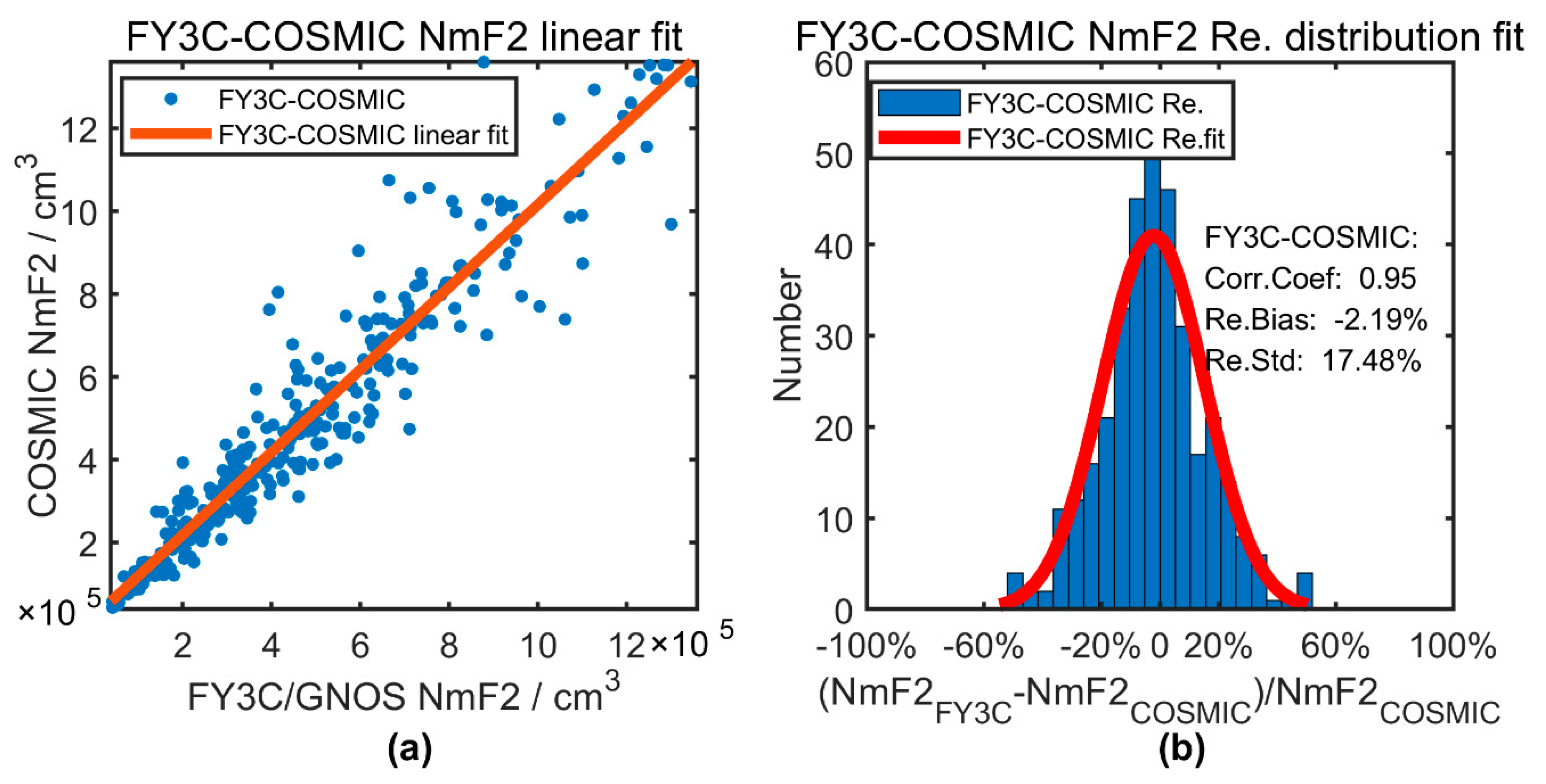
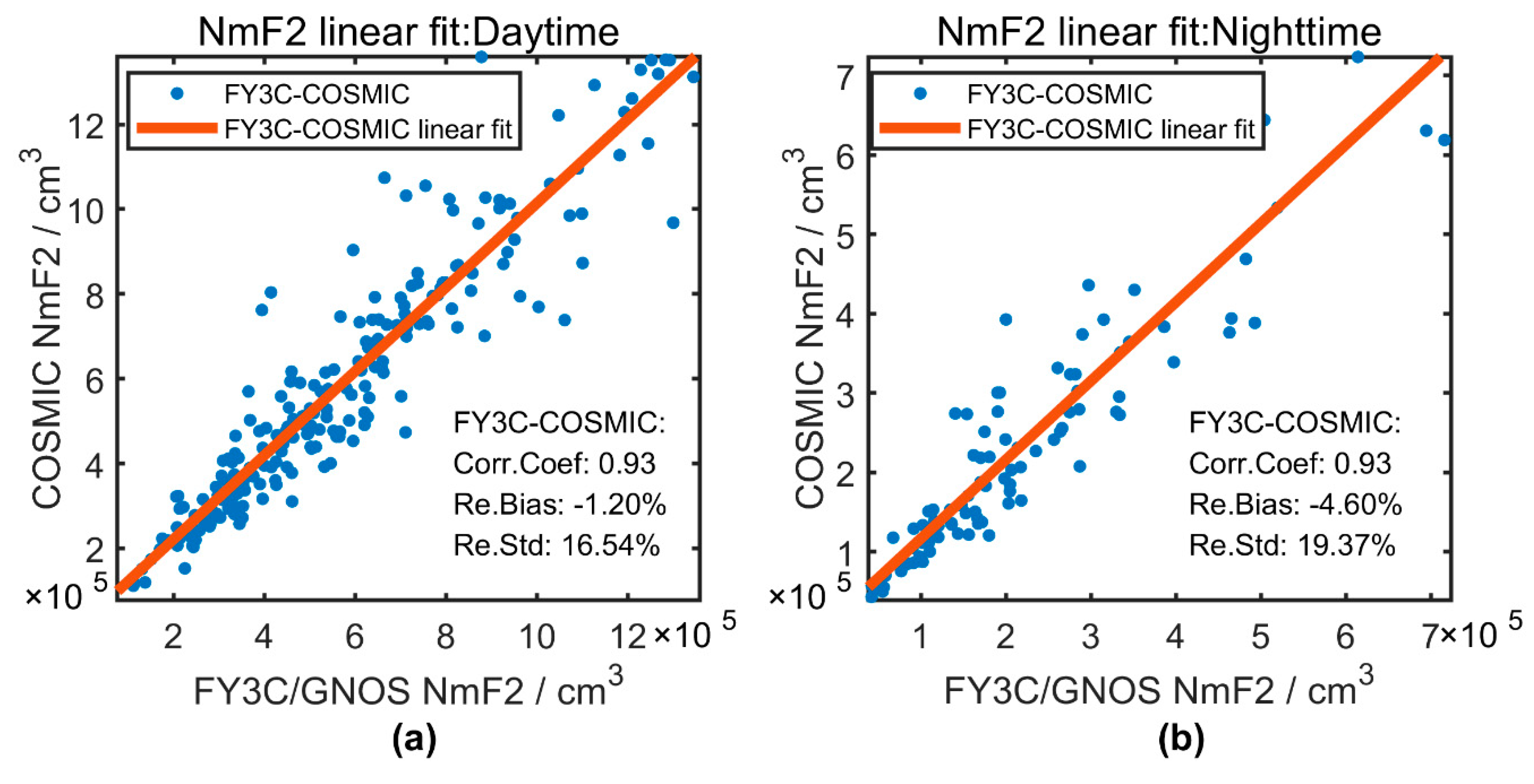
3.1.1. Error Analysis of NmF2 between FY3C/GNOS and COSMIC

The linear fit and statistical error distribution of 346 NmF2 data pairs between FY3C/GNOS and COSMIC during 2016.035 and 2017.035 are presented in Figure 2a,b, respectively. The correlation coefficient of NmF2 data pairs, bias and std of relative errors of NmF2 data pairs are shown in Figure 2b, which are 0.95, −2.19%, and 17.48%, respectively, we can also see that the relative errors of NmF2 between FY3C/GNOS and COSMIC are most concentrated between ±20%, showing a symmetric normal distribution with a mean value around 0. Figure 3a,b demonstrates the linear fit of 245 and 101 NmF2 data pairs between FY3C/GNOS and COSMIC at daytime (0600LT–1800LT) and nighttime (1800LT–0600LT), respectively. During daytime, the correlation coefficient, bias and std of NmF2 between FY3C/GNOS and COSMIC are 0.93, −1.20%, and 16.54%, respectively, during nighttime, the correlation coefficient, bias and std of NmF2 data pairs are 0.93, −4.60%, and 19.37%, respectively.

It can be seen that the correlation coefficients of NmF2 are all above 0.9 during the whole day, daytime and nighttime, showing a good correlation of NmF2 between FY3C/GNOS and COSMIC. Besides, the bias in range of −5% to −1% is accompanied by the std between 16% and 20%, which eliminates the systematic offsets between FY3C/GNOS and COSMIC. The overall std of 17.48% and the bias of −2.19% show the good precision consistency of two different IRO products between FY3C/GNOS and COSMIC. Besides, the precision consistency of NmF2 deteriorated at nighttime compared to daytime and whole day.

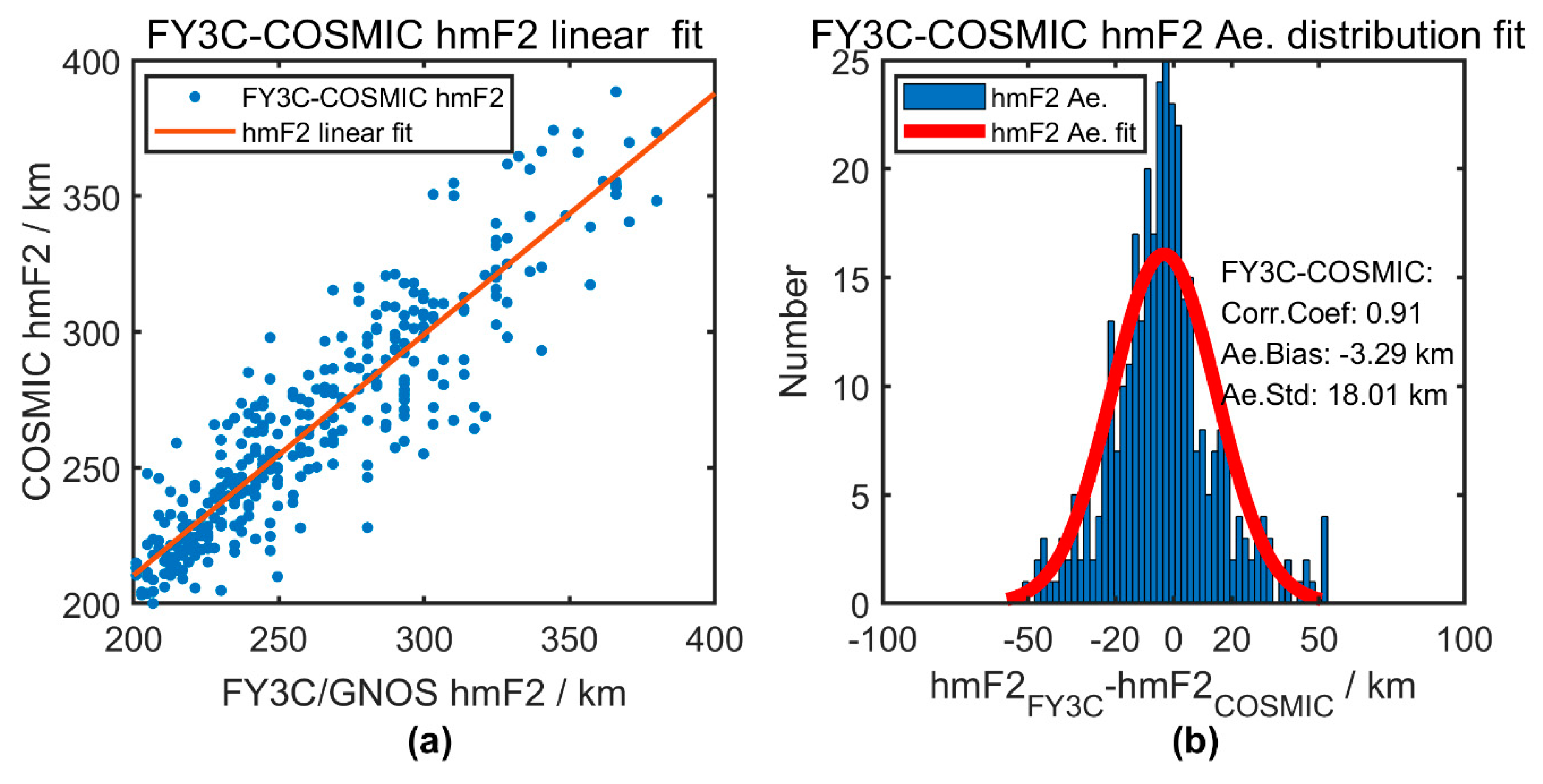
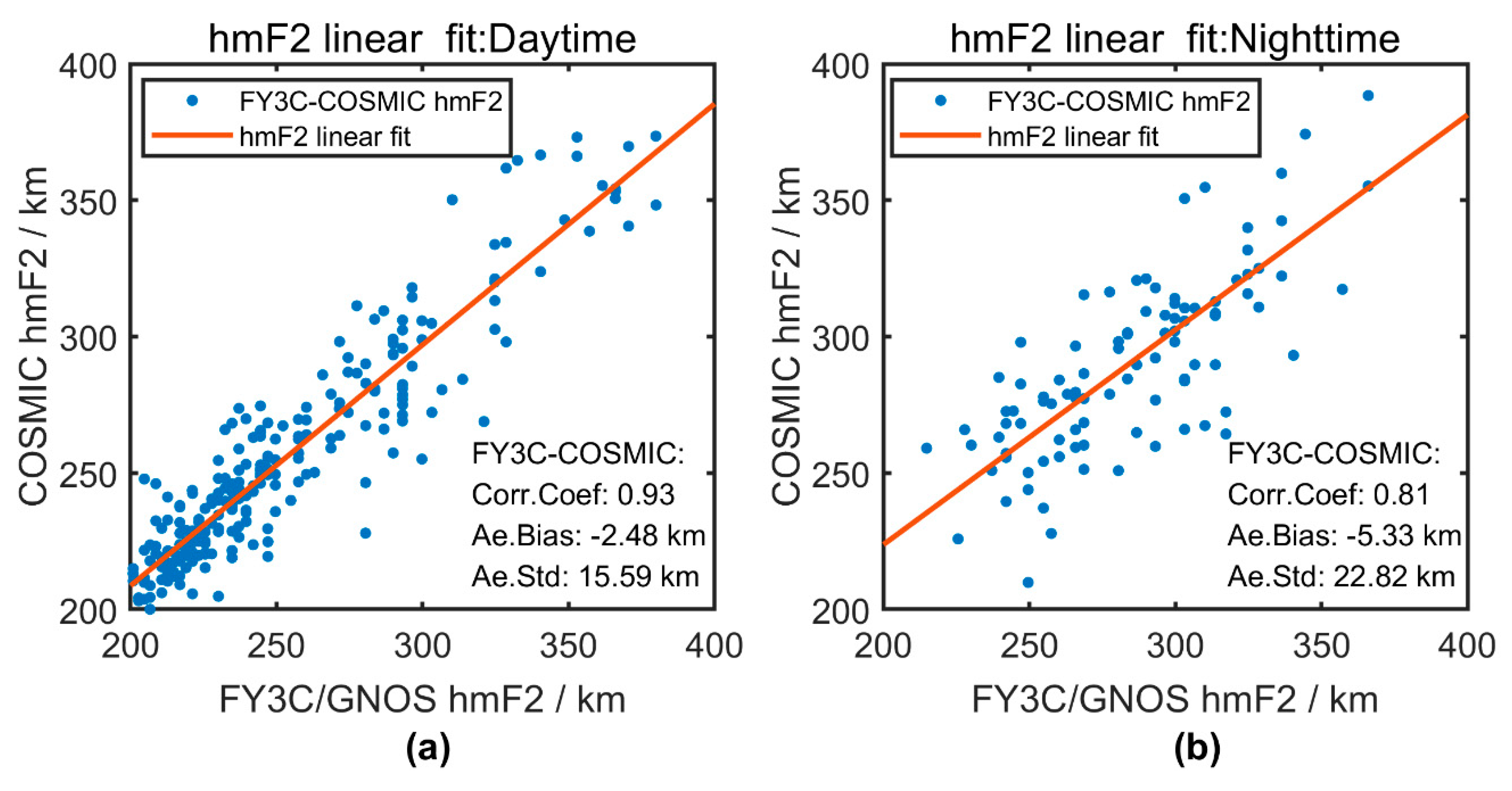
3.1.2. Error Analysis of hmF2 between FY3C/GNOS and COSMIC

Figure 4a,b depicts the linear fit and statistical error distribution of hmF2 between FY3C/GNOS and COSMIC, respectively. As can be seen in Figure 4b, the correlation coefficient of hmF2 data pairs, bias, and std of absolute errors of hmF2 data pairs are 0.91, −3.29 km, and 18.01 km, respectively, and the absolute errors of hmF2 are most focused within ±20 km, showing a symmetric normal distribution with an average value around 0. Linear fits of hmF2 at daytime(0600LT–1800LT) and nighttime(1800LT–0600LT) are depicted in Figure 5a,b, respectively. During daytime, the correlation coefficient, bias, and std of hmF2 are 0.93, −2.48 km, and 15.59 km, respectively, during nighttime, the correlation coefficient, bias, and std of hmF2 are 0.81, −5.33 km, and 22.82 km, respectively.

As can be seen in Figure 4 and Figure 5, the correlation coefficients of hmF2 are all above 0.9 though exceptions do exist at nighttime, which shows a good correlation of hmF2 between FY3C/GNOS and COSMIC. In addition, the bias in range of −6 to −2 km with the std between 15 and 23 km indicates the little significance of systematic offset between FY3C/GNOS and COSMIC. It can be seen that the overall std and bias are 18.01 and −3.29 km, respectively, showing that the hmF2 between FY3C/GNOS and COSMIC are highly agreeable. Similar to NmF2, the precision agreement of hmF2 also deteriorated severely at nighttime.

3.2. Verification of FY3C/GNOS IRO Products in Ionospheric Climatology with COSMIC

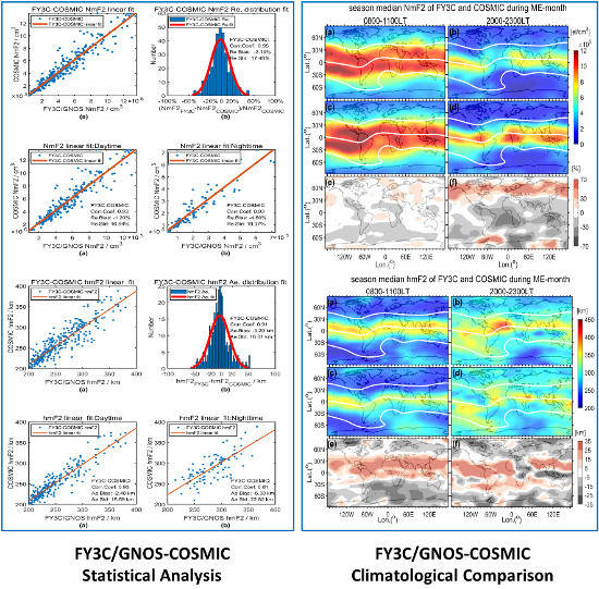
3.2.1. Ionospheric Climatological Characteristics of NmF2 between FY3C/GNOS and COSMIC

We present the global distribution of season median NmF2 of FY3C/GNOS and COSMIC and their relative differences at daytime(0800–1100LT) and nighttime (2000LT–2300LT) during ME-month, JS-month, SE-month, and DS-month from Figure 6, Figure 7, Figure 8 and Figure 9, respectively, thus the consistency and inconsistency of NmF2 morphology between FY3C/GNOS and COSMIC can be obtained intuitively. It can be clearly seen from Figure 6a–d, Figure 7a–d, Figure 8a–d and Figure 9a–d that the season median NmF2 of COSMIC are higher than those of FY3C/GNOS regardless of whether it was daytime or nighttime, especially in equinoxes of ME-month and SE-month. Other global ionospheric climatological characteristics of NmF2 presented by FY3C/GNOS and COSMIC are as follows:

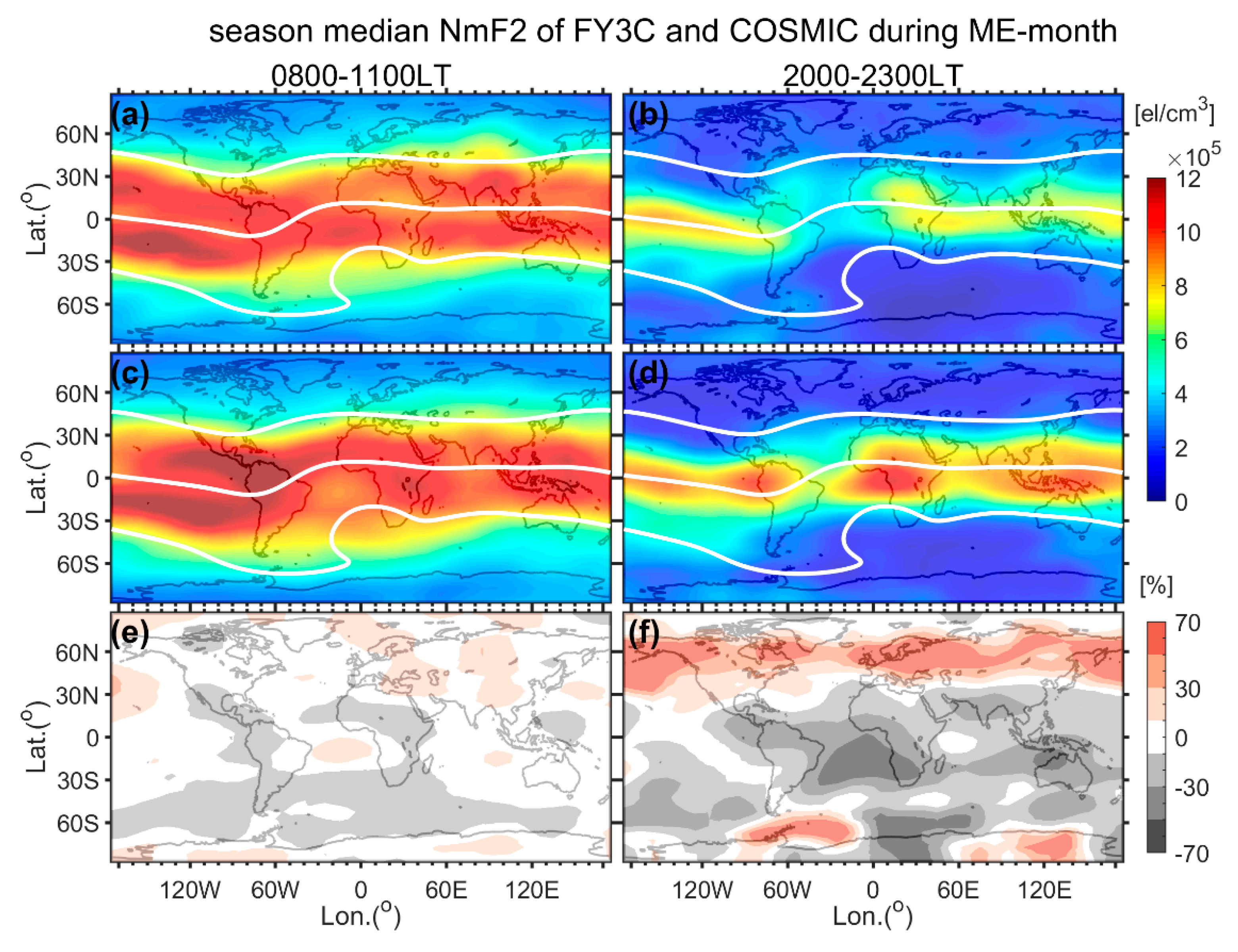
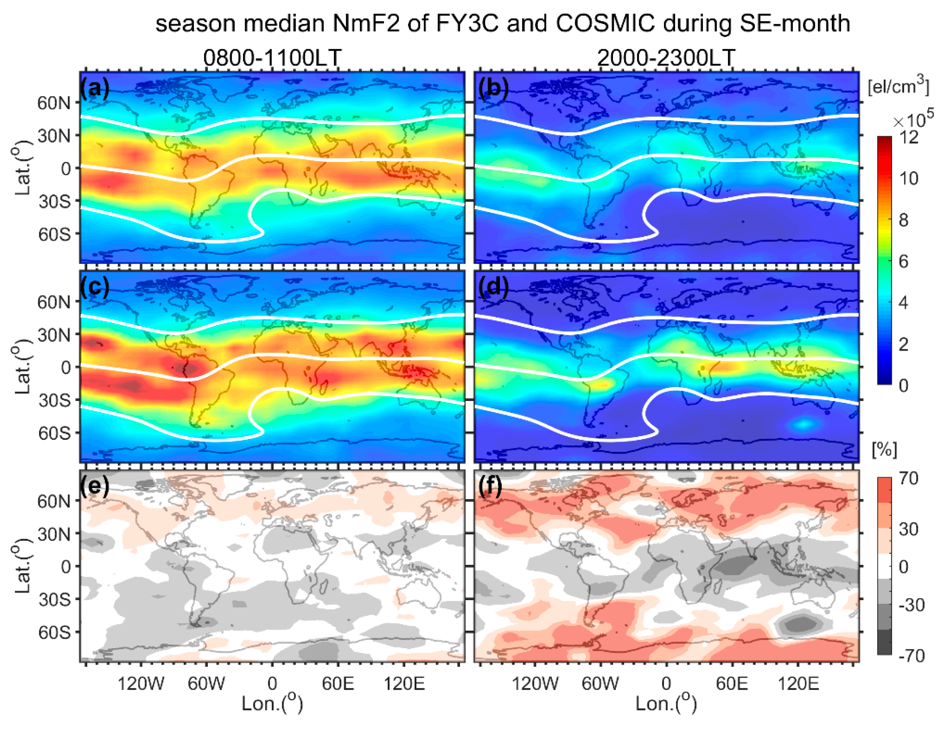
• It can be clearly seen from Figure 6, Figure 7, Figure 8 and Figure 9 that the equatorial ionospheric anomalies (EIAs) are reflected in NmF2 of both FY3C/GNOS and COSMIC and are most obvious at daytime, which appears as an electron density trough along the magnetic equator sandwiched by two high electron density strips [57]. Moreover, the EIA exhibited by COSMIC are more pronounced than that of FY3C/GNOS.
• The daytime NmF2 observed by FY3C/GNOS and COSMIC during equinoxes (ME-month and SE-month) are visibly higher than those in solstices (JS-month and DS-month), which is a typical feature of the semiannual anomaly/asymmetry [46]. The daytime NmF2 of COSMIC are higher than that of FY3C/GNOS, either.
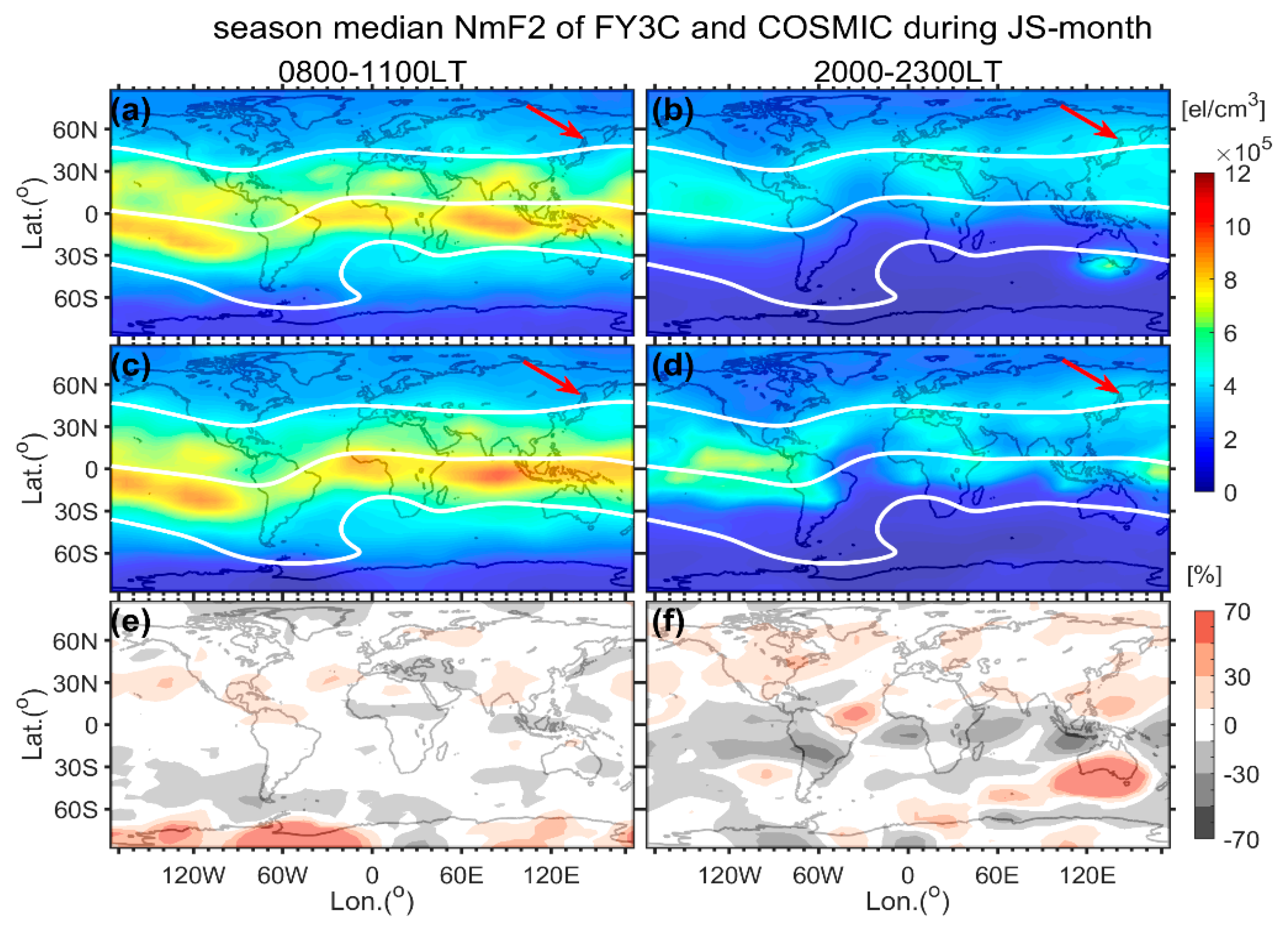
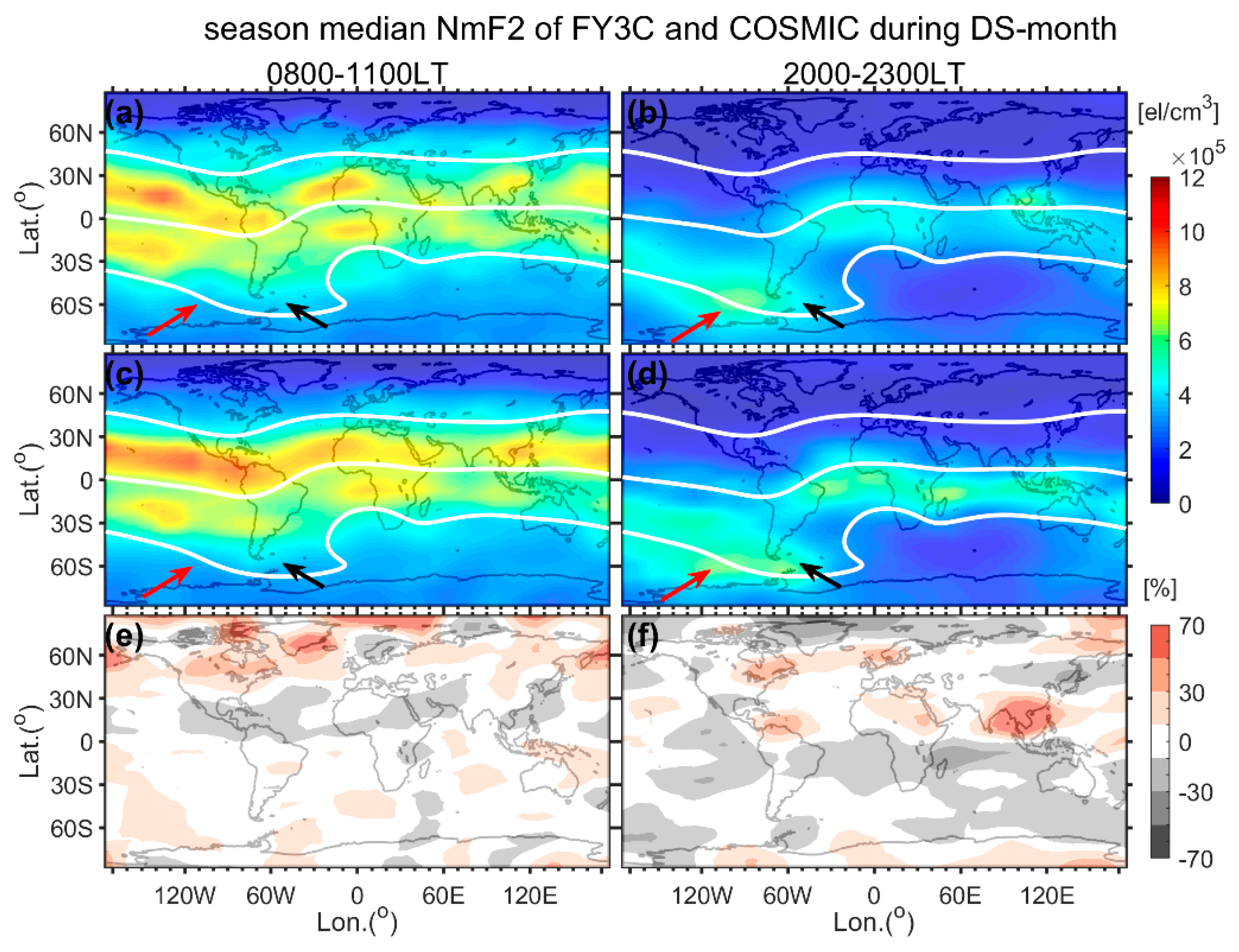
• The daytime NmF2 of FY3C/GNOS and COSMIC during DS-month shows more evident EIA structures than those in JS-month, and the magnitude of NmF2 observed by FY3C/GNOS and COSMIC in DS-month are about 16% and 20% larger than NmF2 in JS-month, respectively. The phenomenon that NmF2 in December solstice are higher than that in June solstice is known as annual anomaly [58].
• The nighttime NmF2 probed by FY3C/GNOS and COSMIC both show peak longitude structures during ME-month, which was also observed in work of Potula et al. [46], and the peak structures of COSMIC NmF2 are more noticeable than that of FY3C/GNOS.
• Taking into account the NmF2 measurements in both the northern and southern hemisphere, it can be found that at daytime, the NmF2 observed by FY3C/GNOS and COSMIC during ME-month have a more continuous EIA than that in SE-month, at nighttime, the NmF2 during ME-month have more evident peak structures than that in SE-month. Thus, the NmF2 observed in ME-month are higher than that in SE-month regardless of whether it was daytime or nighttime, which is known as equinoctial asymmetry and is most pronounced in the EIA region [59].
• The daytime NmF2 measured by FY3C/GNOS and COSMIC in winter are higher than those in summer, which means that the NmF2 observations in the southern hemisphere are higher than those in the northern hemisphere in JS-month, and the NmF2 in northern hemisphere are higher than those in southern hemisphere in DS-month, this behavior of the ionosphere is the winter anomaly [60].
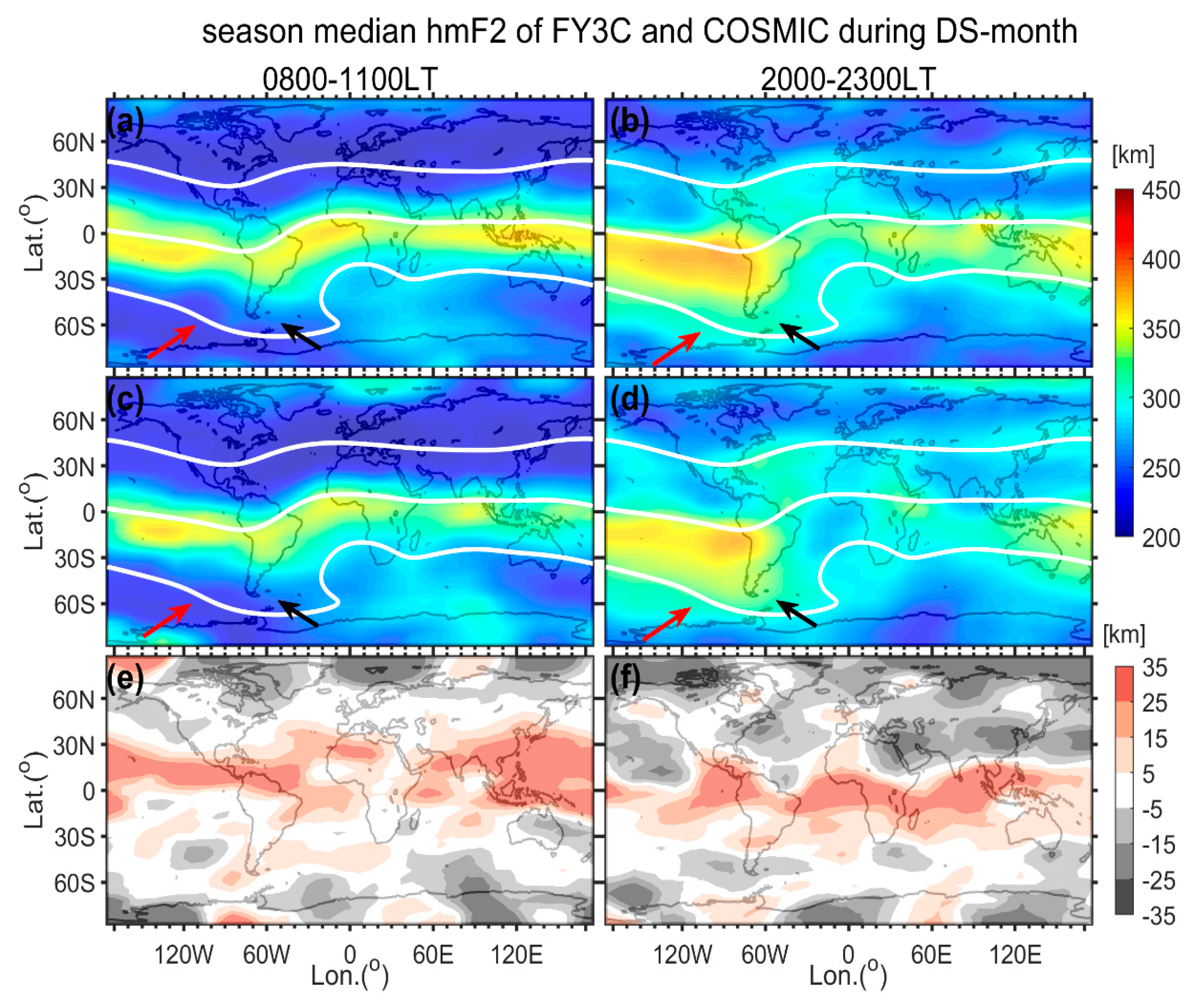
• At nighttime in DS-month, we can see the enhancement of NmF2 of FY3C/GNOS and COSMIC in region of around −60° dip and 50°W–150°W, the nighttime NmF2 enhancement can also be observed in area of around 60° dip and 110°E–160°E in JS-month, which are corresponding to the WSA phenomenon, including the special WSA and the general WSA. The WSA anomaly was first proposed by Penndorf [61], unlike the typical NmF2 diurnal variation, the NmF2 in Weddell Sea area in summer ionosphere showed anomalous nighttime enhancement as denoted by the black arrows in Figure 9b,d, this is known as the special WSA. We can see that the special WSA of FY3C/GNOS is not as pronounced as that of COSMIC. With the enrichment of the global IRO data, many studies [62,63,64] found that the WSA is not limited to the Weddell Sea in summer ionosphere but also occurs in mid-latitude longitude sections in both northern and southern summer ionosphere, where the magnetic equator shifts farthest toward the geographic pole, this is called the general WSA as denoted by the red arrows in Figure 7b,d and Figure 9b,d. It is not hard to see that general WSA in northern summer ionosphere is not as evident as that in southern summer ionosphere.

It can be seen from Figure 6e,f, Figure 7e,f, Figure 8e,f and Figure 9e,f that at nighttime, the NmF2 of FY3C/GNOS are higher than those of COSMIC in mid-high latitudes but lower in low latitudes, especially in equinoxes. The white area (relative error within ±10%) occupies the vast majority of the low-mid latitude regions, showing that NmF2 morphology between FY3C/GNOS and COSMIC are more consistent in these areas.

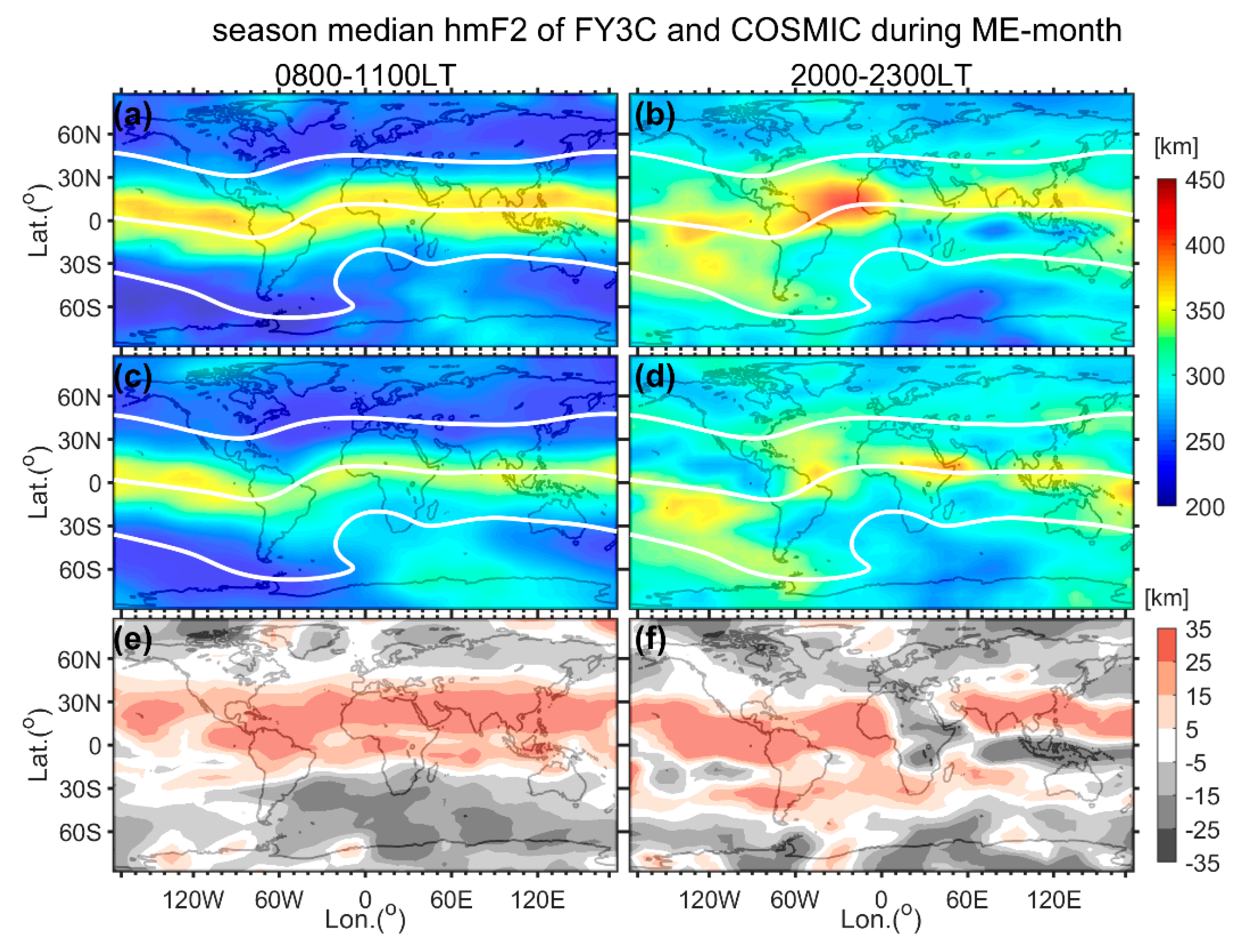
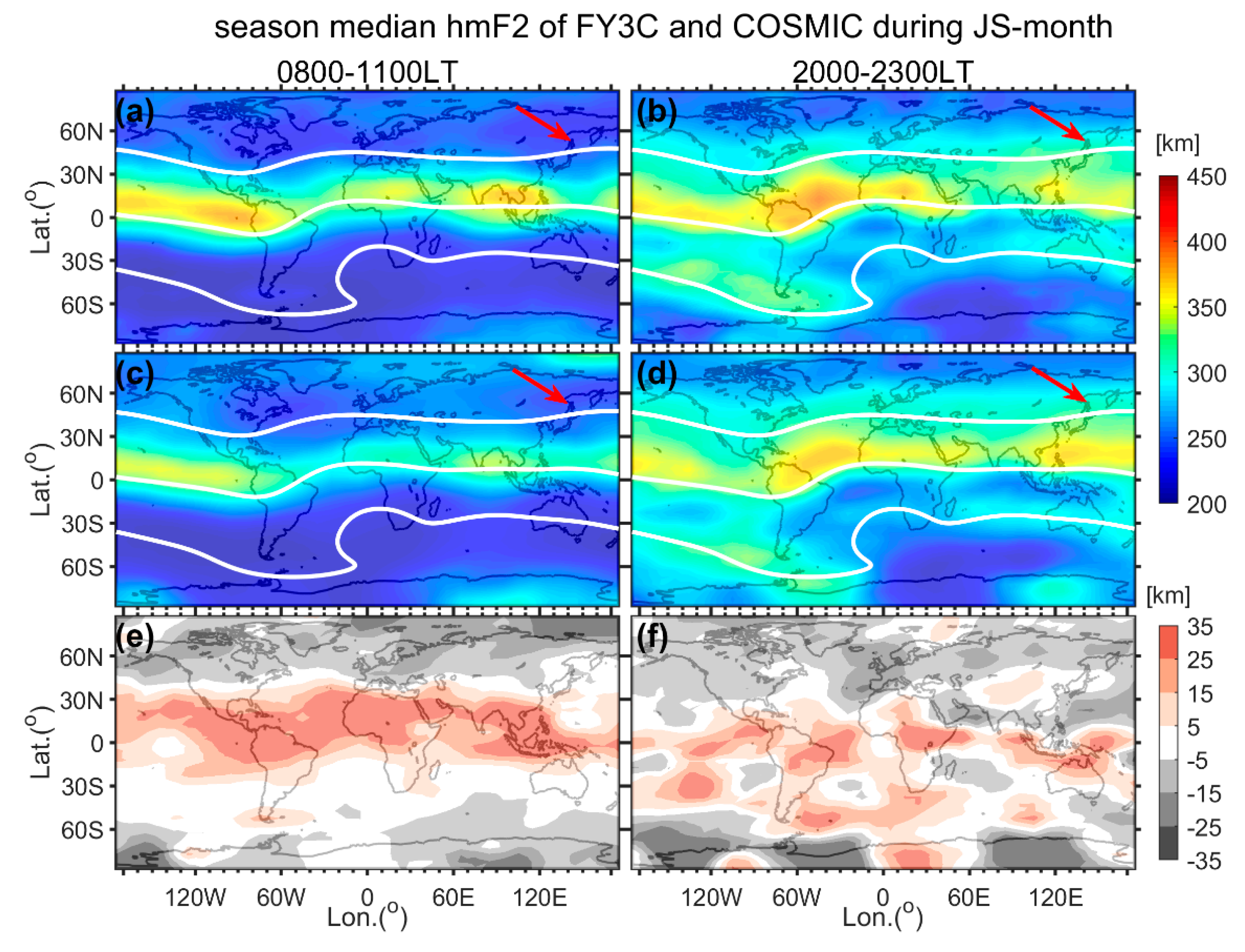
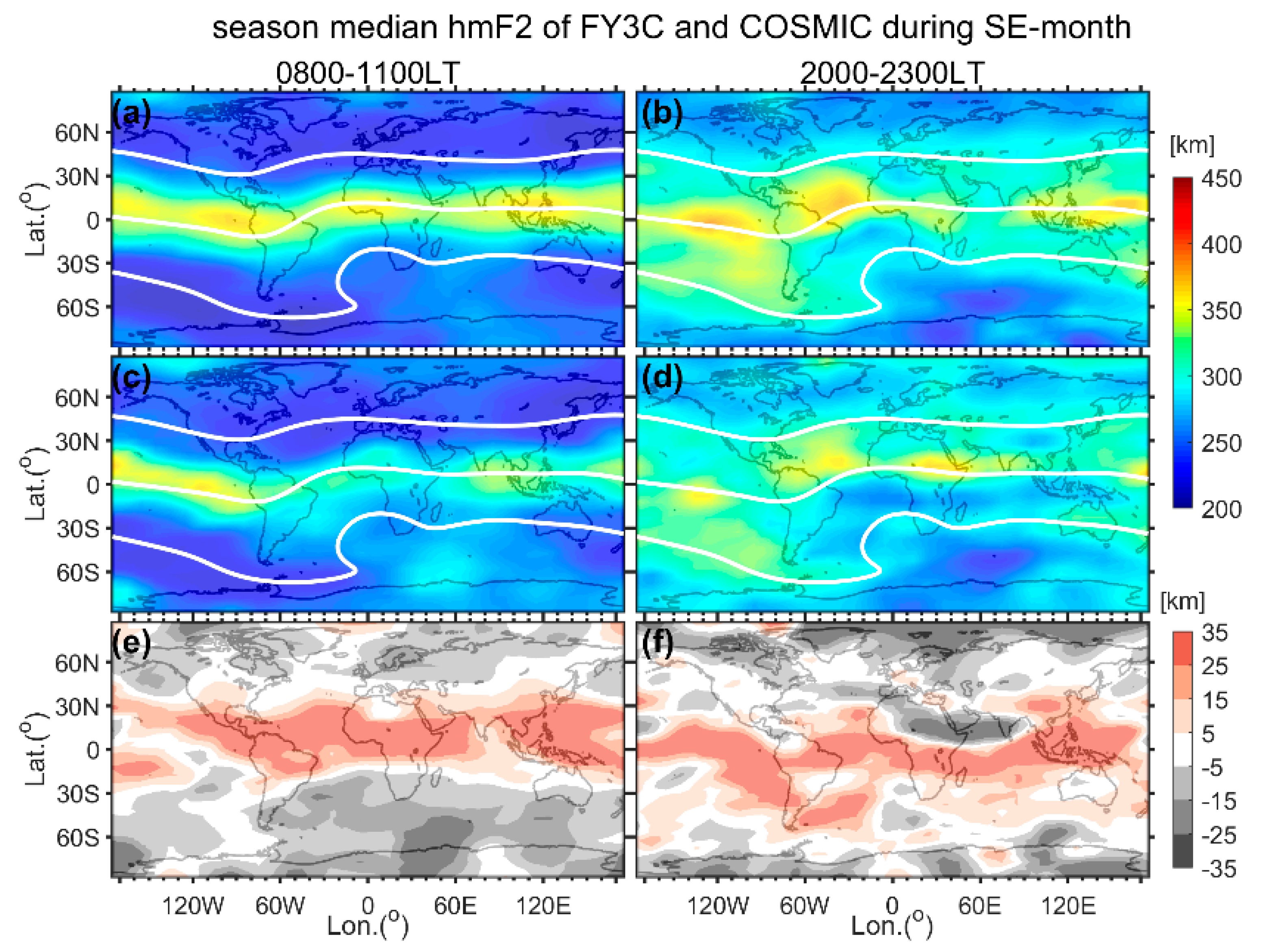
3.2.2. Ionospheric Climatological Characteristics of hmF2 between FY3C/GNOS and COSMIC

The global distribution of season median hmF2 of FY3C/GNOS and COSMIC and their absolute differences at daytime (0800–1100LT) and nighttime (2000LT–2300LT) during ME-month, JS-month, SE-month, and DS-month are presented from Figure 10, Figure 11, Figure 12 and Figure 13, respectively, to depict the hmF2 morphology of FY3C/GNOS and COSMIC intuitively. As can be seen in Figure 10a–d, Figure 11a–d, Figure 12a–d and Figure 13a–d, the season median hmF2 of FY3C/GNOS and COSMIC show good consistency on morphology trend, but there are still some magnitude discrepancies, for example, at daytime, the smaller magnitude of COSMIC hmF2 makes it less continuous in African longitude sector in JS-month and SE-month. At nighttime in the ME-month, FY3C/GNOS exhibits a significant hmF2 peak in the Atlantic region compared to hmF2 of COSMIC. Besides, higher hmF2 of both FY3C/GNOS and COSMIC are most concentrated in low latitude regions at daytime but expand to mid-high latitudes at nighttime, especially in the south Pacific Ocean, showing the global nighttime enhancement of hmF2. One interesting thing is that during daytime when the highest value hmF2 are assembled along the magnetic equator, another relatively high hmF2 appears near the African longitude sector and extends to mid-high latitudes in the southeast direction, and when global hmF2 goes up at nighttime, the aforementioned area is filled by the low value hmF2 again, which are most obvious in ME-month and DS-month. This was also observed in work of Liu et al. [37]. Other hmF2 climatological characteristics are presented as below:

1. hmF2 of FY3C/GNOS and COSMIC are higher in summer hemisphere than that in the winter hemisphere regardless of whether it was daytime or nighttime, that is, the hmF2 in northern ionosphere is higher than that in southern ionosphere in JS-month, and higher in southern ionosphere than that in northern ionosphere in DS-month, which is a typical embodiment of hemispheric asymmetry of hmF2 [65].

2. Generally speaking, the enhancement of NmF2 is usually accompanied by an increasement of hmF2 [35], thus we can observe the WSA phenomenon of hmF2 in either solstice. However, different from NmF2, hmF2 WSA also appeared in winter hemisphere and equinoxes, and the hmF2 of FY3C/GNOS and COSMIC show a more significant WSA characteristics than that of NmF2.

From Figure 10e,f, Figure 11e,f, Figure 12e,f and Figure 13e,f we can see that at nighttime, the hmF2 of FY3C/GNOS are significantly higher than those of COSMIC in low latitudes but lower in mid-high latitudes, which is exactly opposite to NmF2 differences between FY3C/GNOS and COSMIC mentioned before. Additionally, the white area (absolute error within ±10 km) occupies the majority of the mid-latitude region, indicating the better consistency of hmF2 morphology between FY3C/GNOS and COSMIC in mid-latitudes.

4. Discussion

We matched NmF2/hmF2 of FY3C/GNOS and COSMIC into data pairs, the correlation coefficients of both NmF2 and hmF2 data pairs are above 0.9, and the stds of NmF2 and hmF2 are 17.48% and 18.01%, respectively, which are comparable and even better than the statistical error between FY3C/GNOS and ionosondes, thus the precision of NmF2/hmF2 of FY3C/GNOS are verified successfully by comparison with COSMIC. However, at nighttime, the stds of both NmF2 and hmF2 data pairs are worse than that at daytime and during the whole day, indicating the deteriorated consistency of NmF2/hmF2 at nighttime. This may be caused by the lack of the strong daytime photochemical control in F2 layer at nighttime. Under the strong photochemical control at daytime, the carrier phase observation is not affected by the irregularities too much. However, at nighttime, the absence of strong photochemical control gives an opportunity to the daytime hold-over plasma bubbles [66], thus RO signals in different directions are randomly modulated when passing through the irregularities, resulting in discrepancies of NmF2/hmF2 between FY3C/GNOS and COSMIC at nighttime.

From the ionospheric climatological characteristics of NmF2 in four seasons we can see that the ionospheric morphology of FY3C/GNOS and COSMIC are highly agreeable, both showing the typical ionospheric features such as EIA, annual anomaly, semiannual anomaly, winter anomaly, WSA, and so on. The occurrences of these phenomena are closely related to ionospheric dynamics, neutral composition, diurnal tides, solar activity, thermospheric winds, geomagnetic field, and other factors [67,68,69,70,71,72,73,74]. For example, EIA is mainly caused by the equatorial fountain effect driven by E×B drift, which lifts the plasma along the magnetic equator upward to higher latitudes, depleting the plasma in the ionization concentration region, namely, the magnetic equatorial region, thus forming two EIA crests on both hemispheres [67,68,69]. Meanwhile, the amplitude variation of EIA has a lot to do with the semiannual anomaly. The semiannual anomaly seems to abide by the E×B drift modulated by the semiannual variation of the diurnal tide in thermosphere [46], and the amplitude of the semiannual anomaly is positively correlated with solar activity [74]. In addition, Gowtam [70] observed that the winter anomaly is limited at low-latitudes from 0800LT to 1100LT and is almost absent in mid-latitudes in the LSA period, which is consistent with what was revealed in our work. It is considered that the winter anomaly is directly related to the global change of [O]/[N2] ratio, which is the result of heating of the summer hemisphere causing some lighter neutral atmospheric compositions to form convection with the winter hemisphere [58,70,71]. Identical to general WSA observed in our work, the similar anomaly of TEC in the southeastern Pacific Ocean in summer hemisphere is also observed in work of Horvath et al. [72,73], in which the TEC enhancement appears between 2200LT and 2400LT. The present work proposes that the mechanism of WSA phenomenon is most linked to thermospheric wind and regulation of the magnetic field [36].

The season pattern of hmF2 is pretty simple, regulated by an annual variation peaking in local summer [75]. The global ionospheric climatological characteristics of hmF2 measured by FY3C/GNOS are also highly consistent with that of COSMIC, such as hemispheric asymmetry, WSA. Existing studies reported that the hemispheric asymmetry of hmF2 is regulated by the hemispherical asymmetric neutral winds, in which the neutral winds crossing the equator will transport the plasma to the opposite hemisphere, producing the hemispherical asymmetry in solstices [65,76]. Interestingly, the WSA of hmF2 appears not only in nighttime of summer, but also in nighttime of winter and equinoxes. This phenomenon has much to do with the general global rise of hmF2 at nighttime, and the nighttime enhancement of hmF2 is inseparable from changes of magnetic composition and winds [36].

In addition to these highly matched ionospheric climatological features of NmF2/hmF2 between FY3C/GNOS and COSMIC, there are also some minor differences in magnitude of ionospheric climatological characteristics, which may be caused by the different directionalities of occultation rays of FY3C/GNOS and COSMIC and the quantity difference of NmF2/hmF2 in data grids.

We can see from the differences of NmF2/hmF2 between FY3C/GNOS and COSMIC that they both have good consistency of climatological morphology in the mid-latitude region. This is consistent with the general rule of Abel inversion algorithm [77]. In mid-latitudes, the horizontal uniformity of the electron density is better, since the Abel inversion is based on the assumption of local spherical symmetry of the electron density, the inconsistency of morphology in mid-latitudes will be smaller compared to other regions.

5. Conclusions

In this work, we presented season median NmF2/hmF2 observed by FY3C/GNOS and COSMIC during 2016.035 and 2017.035 in four seasons and found that the global ionospheric climatological characteristics probed by FY3C/GNOS are highly consistent with that of COSMIC in typical ionospheric features like the EIA, semiannual anomaly, annual anomaly, winter anomaly, WSA, and so on, though minor discrepancies do exist like the magnitude differences of longitude peak structures and WSA, which shows the significance of the IRO products of FY3C/GNOS in ionospheric climatology study. Besides, this work also for the first time verifies the precision of NmF2/hmF2 of FY3C/GNOS by matching with that of the same type space-based occultation project, COSMIC. The results show that the systematic errors, namely, the biases of NmF2/hmF2 between FY3C/GNOS and COSMIC are close to 0, thus negligible, the overall correlation coefficient and std of NmF2 between FY3C/GNOS and COSMIC is 0.95 and 17.48%, respectively, and the overall correlation coefficient and std of hmF2 is 0.91 and 18.01 km, respectively, demonstrating the decent accuracy consistency of IRO product between FY3C/GNOS and COSMIC.

Due to the limitation of the number of occultation channels, FY3C/GNOS can only observe about 300 (just for GPS) ionospheric occultation events per day. Therefore, FY3D/GNOS launched in 2017 was enhanced in number of occultation channels and antenna coverage, thus increasing the observed number of daily ionospheric occultation events to about 500 (just for GPS). With the enhancement of the observation capability of GNOS payload and the gradual implementation of the 3+1 constellation network established by FY3 series satellites (E, F, G and R) [4], the FY3 series occultation project will make more contributions to the international ionospheric climatology research.

References

1. Burns, A.G.; Solomon, S.C.; Wang, W.; Qian, L.; Zhang, Y.; Paxton, L.J. Daytime climatology of ionospheric NmF2 and hmF2 from COSMIC data: IONOSPHERIC CLIMATOLOGY. J. Geophys. Res. 2012, 117, A09315. [Google Scholar] [CrossRef]
2. Wu, X.C. Radio Occultation Technique for Ionosphere Detection. Ph.D. Thesis, University of Chinese Academy of Sciences, Beijing, China, 2008. [Google Scholar]
3. Yang, G.; Sun, Y.; Bai, W.; Zhang, X.; Liu, C.; Meng, X.; Bi, Y.; Wang, D.; Zhao, D. Validation results of NmF2 and hmF2 derived from ionospheric density profiles of GNOS on FY-3C satellite. Sci. China Technol. Sci. 2018, 61, 1372–1383. [Google Scholar] [CrossRef]
4. Bai, W.; Sun, Y.; Xia, J.; Tan, G.; Cheng, C.; Yang, G.; Du, Q.; Wang, X.; Zhao, D.; Tian, Y.; et al. Validation results of maximum S4 index in F-layer derived from GNOS on FY3C satellite. GPS Solut. 2019, 23, 19. [Google Scholar] [CrossRef]
5. Gong, X.Y. Research on GNSS Atmospheric Radio Occultation Technique. Ph.D. Thesis, University of Chinese Academy of Sciences, Beijing, China, 2008. [Google Scholar]
6. Zhao, Y. GNSS Ionospheric Occultation Inversion and Its Application. Ph.D. Thesis, WuHan University, Hubei, China, 2011. [Google Scholar]
7. Ware, R.; Exner, M.; Feng, D.; Gorbunov, M.; Hardy, K.; Herman, B.; Kuo, Y.; Meehan, T.; Melbourne, W.; Rocken, C.; et al. GPS Sounding of the Atmosphere from Low Earth Orbit: Preliminary Results. Bull. Am. Meteor. Soc. 1996, 77, 19–40. [Google Scholar] [CrossRef]
8. Schreiner, W.S.; Sokolovskiy, S.V.; Rocken, C.; Hunt, D.C. Analysis and validation of GPS/MET radio occultation data in the ionosphere. Radio Sci. 1999, 34, 949–966. [Google Scholar] [CrossRef]
9. Tsuda, T.; Nishida, M.; Rocken, C.; Ware, R.H. A Global Morphology of Gravity Wave Activity in the Stratosphere Revealed by the GPS Occultation Data (GPS/MET). J. Geophys. Res. Atmos. 2000, 105, 7257–7273. [Google Scholar] [CrossRef]
10. Rocken, C.; Anthes, R.; Exner, M.; Hunt, D.; Sokolovskiy, S.; Ware, R.; Gorbunov, M.; Schreiner, W.; Feng, D.; Herman, B.; et al. Analysis and validation of GPS/MET data in the neutral atmosphere. J. Geophys. Res. 1997, 102, 29849–29866. [Google Scholar] [CrossRef]
11. Kursinski, E.R.; Hajj, G.A.; Schofield, J.T.; Linfield, R.P.; Hardy, K.R. Observing Earth′s atmosphere with radio occultation measurements using the Global Positioning System. J. Geophys. Res. 1997, 102, 23429–23465. [Google Scholar] [CrossRef]
12. Wickert, J.; Reigber, C.; Beyerle, G.; König, R.; Marquardt, C.; Schmidt, T.; Grunwaldt, L.; Galas, R.; Meehan, T.K.; Melbourne, W.G.; et al. Atmosphere sounding by GPS radio occultation: First results from CHAMP. Geophys. Res. Lett. 2001, 28, 3263–3266. [Google Scholar] [CrossRef]
13. Jakowski, N.; Wehrenpfennig, A.; Heise, S.; Reigber, C.; Lühr, H.; Grunwaldt, L.; Meehan, T.K. GPS radio occultation measurements of the ionosphere from CHAMP: Early results. Geophys. Res. Lett. 2002, 29, 95-1–95-4. [Google Scholar] [CrossRef]
14. Schmidt, T.; Heise, S.; Wickert, J.; Beyerle, G.; Reigber, C. GPS radio occultation with CHAMP and SAC-C: Global monitoring of thermal tropopause parameters. Atmos. Chem. Phys. 2005, 5, 1473–1488. [Google Scholar] [CrossRef]
15. Jakowski, N.; Tsybulyal, K.; Mielich, J.; Belehaki, A.; Altadill, D.; Jodogne, J.-C.; Zolesi, B. Validation of GPS Ionospheric Radio Occultation results onboard CHAMP by Vertical Sounding Observations in Europe. In Earth Observation with CHAMP; Reigber, C., Lühr, H., Schwintzer, P., Wickert, J., Eds.; Springer-Verlag: Berlin/Heidelberg, Germany, 2005; pp. 447–452. [Google Scholar] [CrossRef]
16. Schreiner, W.; Rocken, C.; Sokolovskiy, S.; Syndergaard, S.; Hunt, D. Estimates of the precision of GPS radio occultations from the COSMIC/FORMOSAT-3 mission. Geophys. Res. Lett. 2007, 34. [Google Scholar] [CrossRef]
17. Liou, Y.A.; Pavelyev, A.G.; Liu, S.F.; Pavelyev, A.A.; Yen, N.; Huang, C.Y.; Chen, J.F. FORMOSAT-3/COSMIC GPS Radio Occultation Mission: Preliminary Results. IEEE Trans. Geosci. Remote Sens. 2007, 45, 3813–3826. [Google Scholar] [CrossRef]
18. Lin, C.H.; Liu, J.Y.; Fang, T.W.; Chang, P.Y.; Tsai, H.F.; Chen, C.H.; Hsiao, C.C. Motions of the equatorial ionization anomaly crests imaged by FORMOSAT-3/COSMIC. Geophys. Res. Lett. 2007, 34. [Google Scholar] [CrossRef]
19. Sokolovskiy, S.V.; Rocken, C.; Lenschow, D.H.; Kuo, Y.H.; Anthes, R.A.; Schreiner, W.S.; Hunt, D.C. Observing the moist troposphere with radio occultation signals from COSMIC. Geophys. Res. Lett. 2007, 34. [Google Scholar] [CrossRef]
20. Anthes, R.A.; Bernhardt, P.A.; Chen, Y.; Cucurull, L.; Dymond, K.F.; Ector, D.; Healy, S.B.; Ho, S.P.; Hunt, D.C.; Kuo, Y.H.; et al. The COSMIC/FORMOSAT-3 Mission: Early Results. Bull. Am. Meteor. Soc. 2008, 89, 313–334. [Google Scholar] [CrossRef]
21. Bi, Y.; Yang, Z.; Zhang, P.; Sun, Y.; Bai, W.; Du, Q.; Yang, G.; Chen, J.; Liao, M. An introduction to China FY3 radio occultation mission and its measurement simulation. Adv. Space Res. 2012, 49, 1191–1197. [Google Scholar] [CrossRef]
22. Liao, M.; Zhang, P.; Yang, G.L.; Bi, Y.M.; Liu, Y.; Bai, W.H.; Meng, X.G.; Du, Q.F.; Sun, Y.Q. Preliminary validation of refractivity from a new radio occultation sounder GNOS/FY-3C. Atmos. Meas. Tech. Discuss. 2015, 8, 9009–9044. [Google Scholar] [CrossRef]
23. Cai, Y.; Bai, W.; Wang, X.; Sun, Y.; Du, Q.; Zhao, D.; Meng, X.; Liu, C.; Xia, J.; Wang, D.; et al. In-orbit performance of GNOS on-board FY3-C and the enhancements for FY3-D satellite. Adv. Space Res. 2017, 60, 2812–2821. [Google Scholar] [CrossRef]
24. Wang, X.; Sun, Y.; Du, Q.; Bai, W.; Wang, D.; Cai, Y.; Wu, D.; Li, W.; Meng, X.; Wu, C.; et al. Improvements of GNOS on-board FY3D. In Proceedings of the 2016 International Technical Meeting of the Institute of Navigation, Monterey, CA, America, 25–28 January 2016; pp. 829–835. [Google Scholar]
25. Wang, D.; Tian, Y.; Sun, Y.; Du, Q.; Wang, X.; Bai, W.; Meng, X.; Cai, Y.; Wu, C.; Liu, C.; et al. Preliminary in-Orbit Evaluation of Gnos on FY3D Satellite. In Proceedings of the IGARSS 2018–2018 IEEE International Geoscience and Remote Sensing Symposium (IGARSS 2018), Valencia, Spanish, 22–27 July 2018; pp. 9161–9163. [Google Scholar] [CrossRef]
26. Ho, S.; Yue, X.; Zeng, Z.; Ao, C.O.; Huang, C.Y.; Kursinski, E.R.; Kuo, Y.-H. Applications of COSMIC Radio Occultation Data from the Troposphere to Ionosphere and Potential Impacts of COSMIC-2 Data. Bull. Am. Meteor. Soc. 2014, 95, ES18–ES22. [Google Scholar] [CrossRef]
27. Yue, X.; Schreiner, W.S.; Pedatella, N.; Anthes, R.A.; Mannucci, A.J.; Straus, P.R.; Liu, J.Y. Space Weather Observations by GNSS Radio Occultation: From FORMOSAT-3/COSMIC to FORMOSAT-7/COSMIC-2. Space Weather 2014, 12, 616–621. [Google Scholar] [CrossRef]
28. Liu, J.Y.; Chen, S.P.; Yeh, W.H.; Tsai, H.F.; Rajesh, P.K. Worst-Case GPS Scintillations on the Ground Estimated from Radio Occultation Observations of FORMOSAT-3/COSMIC During 2007–2014. Surv. Geophys. 2016, 37, 791–809. [Google Scholar] [CrossRef]
29. McNamara, L.F.; Thompson, D.C. Validation of COSMIC values of foF2 and M (3000) F2 using ground-based ionosondes. Adv. Space Res. 2015, 55, 163–169. [Google Scholar] [CrossRef]
30. Krankowski, A.; Zakharenkova, I.; Krypiak-Gregorczyk, A.; Shagimuratov, I.I.; Wielgosz, P. Ionospheric electron density observed by FORMOSAT-3/COSMIC over the European region and validated by ionosonde data. J. Geod. 2011, 85, 949–964. [Google Scholar] [CrossRef]
31. Anthes, R.A.; Rocken, C.; Kuo, Y.H. Applications of COSMIC to Meteorology and Climate. Terr. Atmos. Ocean. Sci. 2000, 11, 115. [Google Scholar] [CrossRef]
32. Zhao, B.; Wang, M.; Wang, Y.; Ren, Z.; Yue, X.; Zhu, J.; Wan, W.; Ning, B.; Liu, J.; Xiong, B. East-west differences in F-region electron density at midlatitude: Evidence from the Far East region. J. Geophys. Res. Space Phys. 2013, 118, 542–553. [Google Scholar] [CrossRef]
33. Yue, X.; Schreiner, W.S.; Kuo, Y.H.; Hunt, D.C. GNSS Radio Occultation Technique and Space Weather Monitoring. In Proceedings of the 26th International Technical Meeting of the Satellite Division of the Institute of Navigation (ION GNSS+ 2013), Nashvill, TN, USA, 16–20 September 2013. [Google Scholar]
34. Zeng, Z.; Burns, A.; Wang, W.; Lei, J.; Solomon, S.; Syndergaard, S.; Qian, L.; Kuo, Y.H. Ionospheric annual asymmetry observed by the COSMIC radio occultation measurements and simulated by the TIEGCM. J. Geophys. Res. 2008, 113. [Google Scholar] [CrossRef]
35. Burns, A.G.; Zeng, Z.; Wang, W.; Lei, J.; Solomon, S.C.; Richmond, A.D.; Killeen, T.L.; Kuo, Y.H. Behavior of the F2 peak ionosphere over the South Pacific at dusk during quiet summer conditions from COSMIC data. J. Geophys. Res. 2008, 113, A12305.1–A12305.9. [Google Scholar] [CrossRef]
36. He, M.; Liu, L.; Wan, W.; Ning, B.; Zhao, B.; Wen, J.; Yue, X.; Le, H. A study of the Weddell Sea Anomaly observed by FORMOSAT-3/COSMIC. J. Geophys. Res. 2009, 114, A12309. [Google Scholar] [CrossRef] [Green Version]
37. Liu, L.; Le, H.; Chen, Y.; He, M.; Wan, W.; Yue, X. Features of the middle- and low-latitude ionosphere during solar minimum as revealed from COSMIC radio occultation measurements. J. Geophys. Res. 2011, 116, A09307. [Google Scholar] [CrossRef]
38. Yue, X.; Schreiner, W.S.; Kuo, Y.H. A feasibility study of the radio occultation electron density retrieval aided by a global ionospheric data assimilation model. J. Geophys. Res. 2012, 117, A08301. [Google Scholar] [CrossRef] [Green Version]
39. Yue, X.; Schreiner, W.S.; Kuo, Y.H.; Hunt, D.C.; Wang, W.; Solomon, S.C.; Burns, A.G.; Bilitza, D.; Liu, J.Y.; Wan, W.; et al. Global 3-D ionospheric electron density reanalysis based on multisource data assimilation. J. Geophys. Res. 2012, 117, A09325. [Google Scholar] [CrossRef] [Green Version]
40. Pavelyev, A.G.; Liou, Y.A.; Wickert, J.; Schmidt, T.; Pavelyev, A.A.; Liu, S.F. Effects of the ionosphere and solar activity on radio occultation signals: Application to CHAllenging Minisatellite Payload satellite observations. J. Geophys. Res. 2007, 112, A06326. [Google Scholar] [CrossRef] [Green Version]
41. Wang, G.; Shi, J.; Bai, W.; Galkin, I.; Wang, Z.; Sun, Y. Global ionospheric scintillations revealed by GPS radio occultation data with FY3C satellite before midnight during the March 2015 storm. Adv. Space. Res. 2019, 63, 3119–3130. [Google Scholar] [CrossRef]
42. Liu, J.Y.; Chen, Y.I.; Pulinets, S.A.; Tsai, Y.B.; Chuo, Y.J. Seismo-ionospheric signatures prior to M ≥ 6.0 Taiwan earthquakes. Geophys. Res. Lett. 2000, 27, 3113–3116. [Google Scholar] [CrossRef]
43. Ho, Y.Y.; Jhuang, H.K.; Lee, L.C.; Liu, J.Y. Ionospheric density and velocity anomalies before M ≥ 6.5 earthquakes observed by DEMETER satellite. J. Asian Earth Sci. 2018, 166, 210–222. [Google Scholar] [CrossRef]
44. Oyama, K.I.; Chen, C.H.; Bankov, L.; Minakshi, D.; Ryu, K.; Liu, J.Y.; Liu, H. Precursor effect of March 11, 2011 off the coast of Tohoku earthquake on high and low latitude ionospheres and its possible disturbing mechanism. Adv. Space. Res. 2019, 63, 2623–2637. [Google Scholar] [CrossRef]
45. Lin, C.H.; Liu, J.Y.; Cheng, C.Z.; Chen, C.H.; Liu, C.H.; Wang, W.; Burns, A.G.; Lei, J. Three-dimensional ionospheric electron density structure of the Weddell Sea Anomaly. J. Geophys. Res. 2009, 114, A02312. [Google Scholar] [CrossRef] [Green Version]
46. Potula, B.S.; Chu, Y.H.; Uma, G.; Hsia, H.P.; Wu, K.H. A global comparative study on the ionospheric measurements between COSMIC radio occultation technique and IRI model. J. Geophys. Res. 2011, 116, A02310. [Google Scholar] [CrossRef] [Green Version]
47. Lee, W.K.; Kil, H.; Kwak, Y.-S.; Wu, Q.; Cho, S.; Park, J.U. The winter anomaly in the middle-latitude F region during the solar minimum period observed by the Constellation Observing System for Meteorology, Ionosphere, and Climate: WINTER ANOMALY DURING SOLAR MINIMUM. J. Geophys. Res. 2011, 116, A02302. [Google Scholar] [CrossRef]
48. Sripathi, S. COSMIC observations of ionospheric density profiles over Indian region: Ionospheric conditions during extremely low solar activity period. Indian J. Radio Space Phys. 2012, 12, 98–109. [Google Scholar]
49. Bai, W.; Wang, G.; Sun, Y.; Shi, J.; Yang, G.; Meng, X.; Wang, D.; Du, Q.; Wang, X.; Xia, J.; et al. Application of the Fengyun 3 C GNSS occultation sounder for assessing the global ionospheric response to a magnetic storm event. Atmos. Meas. Tech. 2019, 12, 1483–1493. [Google Scholar] [CrossRef] [Green Version]
50. Patel, N.C.; Karia, S.P.; Pathak, K.N. Evaluation of the improvement of IRI-2016 over IRI-2012 at the India low-latitude region during the ascending phase of cycle 24. Adv. Space Res. 2019, 63, 1860–1881. [Google Scholar] [CrossRef]
51. F10.7 cm Radio Emissions|NOAA/NWS Space Weather Prediction Center. Available online: https://www.swpc.noaa.gov/phenomena/f107-cm-radio-emissions (accessed on 20 October 2019).
52. Bartels, J.; Heck, N.H.; Johnson, H.F. The three-hour-range index measuring geomagnetic activity. J. Geophys. Res. 1939, 44, 411–454. [Google Scholar] [CrossRef]
53. Yang, K.F.; Chu, Y.H.; Su, C.L.; Ko, H.T.; Wang, C.Y. An Examination of FORMOSAT-3/COSMIC Ionospheric Electron Density Profile: Data Quality Criteria and Comparisons with the IRI Model. Terr. Atmos. Ocean. Sci. 2009, 20, 193. [Google Scholar] [CrossRef] [Green Version]
54. Ma, X.X. Study on the distribution characteristics and seismic response of ionosphere using COSMIC occultation data. Recent Dev. World Seismol. 2015, 3, 47–48. (In Chinese) [Google Scholar] [CrossRef]
55. Hu, L.; Ning, B.; Liu, L.; Zhao, B.; Li, G.; Wu, B.; Huang, Z.; Hao, X.; Chang, S.; Wu, Z. Validation of COSMIC ionospheric peak parameters by the measurements of an ionosonde chain in China. Ann. Geophys. 2014, 32, 1311–1319. [Google Scholar] [CrossRef] [Green Version]
56. Limberger, M.; Hernández-Pajares, M.; Aragón-Ángel, A.; Altadill, D.; Dettmering, D. Long-term comparison of the ionospheric F2 layer electron density peak derived from ionosonde data and Formosat-3/COSMIC occultations. J. Space Weather Space Clim. 2015, 5, A21. [Google Scholar] [CrossRef]
57. Berkner, L.V.; Wells, H.W.; Seaton, S.L. Characteristics of the upper region of the ionosphere. J. Geophys. Res. 1936, 41, 173–184. [Google Scholar] [CrossRef]
58. Torr, M.R.; Torr, D.G. The seasonal behaviour of the F2-layer of the ionosphere. J. Atmos. Terr. Phys. 1973, 35, 2237–2251. [Google Scholar] [CrossRef]
59. Balan, N.; Otsuka, Y.; Fukao, S.; Abdu, M.A.; Bailey, G.J. Annual variations of the ionosphere: A review based on MU radar observations. Adv. Space Res. 2000, 25, 153–162. [Google Scholar] [CrossRef]
60. Duncan, R.A. F-region seasonal and magnetic-storm behaviour. J. Atmos. Terr. Phys. 1969, 31, 59–70. [Google Scholar] [CrossRef]
61. Penndorf, R. The Average Ionospheric Conditions Over the Antarctic. In Geomagnetism and Aeronomy: Studies in the Ionosphere, Geomagnetism and Atmospheric Radio Noise; American Geophysical Union (AGU): Washington, DC, USA, 2013; pp. 1–45. [Google Scholar] [CrossRef]
62. Rishbeth, H.; Mendillo, M. Patterns of F2-layer variability. J. Atmos. Sol-Terr. Phy. 2001, 63, 1661–1680. [Google Scholar] [CrossRef]
63. Chan, K.L.; Colin, L. Global electron density distributions from topside soundings. Proc. IEEE 1969, 57, 990–1004. [Google Scholar] [CrossRef]
64. Rishbeth, H.; Kervin, C. Seasonal changes displayed by F1-layer ionograms. J. Atmos. Terr. Phys. 1968, 30, 1657–1665. [Google Scholar] [CrossRef]
65. Rishbeth, H. How the thermospheric circulation affects the ionospheric F2-layer. J. Atmos. Sol-Terr. Phy. 1998, 60, 1385–1402. [Google Scholar] [CrossRef]
66. Dymond, K.F. Global observations of L band scintillation at solar minimum made by COSMIC. Radio Sci. 2012, 47, RS0L18. [Google Scholar] [CrossRef]
67. Appleton, E.V. Two Anomalies in the Ionosphere. Nature 1946, 157, 691. [Google Scholar] [CrossRef]
68. Duncan, R.A. The equatorial F-region of the ionosphere. J. Atmos. Terr. Phys. 1960, 18, 89–100. [Google Scholar] [CrossRef]
69. Anderson, D.N. A theoretical study of the ionospheric F region equatorial anomaly—I. Theory. Planet. Space Sci. 1973, 21, 409–419. [Google Scholar] [CrossRef]
70. Sai Gowtam, V.; Tulasi Ram, S. Ionospheric winter anomaly and annual anomaly observed from Formosat-3/COSMIC Radio Occultation observations during the ascending phase of solar cycle 24. Adv. Space Res. 2017, 60, 1585–1593. [Google Scholar] [CrossRef]
71. Rishbeth, H.; Setty, C.S.G.K. The F-layer at sunrise. J. Atmos. Terr. Phys. 1961, 20, 263–276. [Google Scholar] [CrossRef]
72. Horvath, I.; Essex, E.A. The Weddell sea anomaly observed with the Topex satellite data. J. Atmos. Sol-Terr. Phy. 2003, 65, 693–706. [Google Scholar] [CrossRef]
73. Horvath, I. A total electron content space weather study of the nighttime Weddell Sea Anomaly of 1996/1997 southern summer with TOPEX/Poseidon radar altimetry. J. Geophys. Res. 2006, 111, A12317. [Google Scholar] [CrossRef] [Green Version]
74. Ma, R.; Xu, J.; Liao, H. The features and a possible mechanism of semiannual variation in the peak electron density of the low latitude F2 layer. J. Atmos. Sol-Terr. Phy. 2003, 65, 47–57. [Google Scholar] [CrossRef]
75. Liu, L.; Zhao, B.; Wan, W.; Ning, B.; Zhang, M.L.; He, M. Seasonal variations of the ionospheric electron densities retrieved from Constellation Observing System for Meteorology, Ionosphere, and Climate mission radio occultation measurements. J. Geophys. Res. 2009, 114, A02302. [Google Scholar] [CrossRef] [Green Version]
76. Luan, X.; Solomon, S.C. Meridional winds derived from COSMIC radio occultation measurements. J. Geophys. Res. 2008, 113, A08302. [Google Scholar] [CrossRef] [Green Version]
77. Yang, G.L.; Sun, Y.Q.; Bai, W.H.; Zhang, X.X.; Yang, Z.D.; Zhang, P.; Tan, G.Y. Beidou navigation satellite system sounding of the ionosphere from FY-3C GNOS: Preliminary results (in Chinese). Chin. J. Space Sci. 2019, 39, 36–45. [Google Scholar] [CrossRef]
Figure 1. Kp variations during 2016.035–2017.035. The red line represents Kp = 4, namely the critical Kp value of a magnetic storm.
Remotesensing 11 02686 g001
Figure 2. Linear fit and statistical error distribution of NmF2 between FengYun-3C (FY3C)/Global Navigation Satellite System occultation sounder (GNOS) and Constellation Observing System for Meteorology, Ionosphere, and Climate (COSMIC) over a whole day during 2016.035 and 2017.035: (a) the linear fit of NmF2 between FY3C/GNOS (horizontal axis) and COSMIC (vertical axis) over a whole day, in which the blue dots represent the matched data pairs of NmF2 and the red line depicts the linear regression fit of NmF2 data pairs; (b) the number (vertical axis) of NmF2 relative errors (horizontal axis) between FY3C/GNOS and COSMIC, in which the red curve represents the distribution fit of the relative errors. The correlation coefficient of NmF2 data pairs, bias, and std of relative errors of matched NmF2 data pairs are also labelled in the right side of (b).
Remotesensing 11 02686 g002
Figure 3. Linear fits of NmF2 between FY3C/GNOS and COSMIC at daytime and nighttime during 2016.035 and 2017.035: (a) the linear fit of NmF2 between FY3C/GNOS (horizontal axis) and COSMIC (vertical axis) at 0600–1800LT, corresponding to daytime; (b) the linear fit of NmF2 at 1800–0600LT, corresponding to nighttime. The correlation coefficient of NmF2 data pairs, the bias, and std of relative errors of matched NmF2 data pairs at daytime and nighttime are presented in the bottom right corner of (a) and (b), respectively.
Remotesensing 11 02686 g003
Figure 4. Linear fit and statistical error distribution of hmF2 between FY3C/GNOS and COSMIC over a whole day during 2016.035 and 2017.035: (a) the linear fit of hmF2 between FY3C/GNOS (horizontal axis) and COSMIC (vertical axis) over a whole day, in which the blue dots represent the matched data pairs of hmF2 and the red line depicts the linear regression fit of hmF2 data pairs; (b) the number (vertical axis) of hmF2 absolute errors (horizontal axis) between FY3C/GNOS and COSMIC, in which the red curve represents the distribution fit of the absolute errors. The correlation coefficient of hmF2 data pairs, bias, and std of absolute errors of matched hmF2 data pairs are also labelled in the right side of (b).
Remotesensing 11 02686 g004
Figure 5. Linear fits of hmF2 between FY3C/GNOS and COSMIC at daytime and nighttime during 2016.035 and 2017.035: (a) the linear fit of hmF2 between FY3C/GNOS (horizontal axis) and COSMIC (vertical axis) at 0600–1800LT, corresponding to daytime; (b) the linear fit of hmF2 at 1800–0600LT, corresponding to nighttime. The correlation coefficient of hmF2 data pairs, the bias, and std of absolute errors of matched hmF2 data pairs at daytime and nighttime are presented in the bottom right corner of (a) and (b), respectively.
Remotesensing 11 02686 g005
Figure 6. Ionospheric climatological characteristics of season median NmF2 observed by FY3C/GNOS and COSMIC and their differences at 0800–1100LT and 2000–2300LT during ME-month (±45 days to March equinox of 2016) from 2016.035 to 2016.125. (a,b) The climatological characteristics of season median NmF2 observed by FY3C/GNOS at 0800–1100LT and 2000–2300LT, respectively. (c,d) The climatological characteristics of season median NmF2 probed by COSMIC at 0800–1100LT and 2000–2300LT, respectively. The dip contours in (a–d) are represented by white curves, which are 60° dip, 0° dip, −60° dip from top to bottom, respectively. (e,f) The relative errors of season median NmF2 between FY3C/GNOS and COSMIC at 0800–1100LT and 2000–2300LT, respectively. The acquisition of NmF2 relative error can be seen in Section 2.2.
Remotesensing 11 02686 g006
Figure 7. Ionospheric climatological characteristics of season median NmF2 observed by FY3C/GNOS and COSMIC and their differences at 0800–1100LT and 2000–2300LT during JS-month (±45 days to June solstice of 2016) from 2016.128 to 2016.218. The red arrow points to the diurnal variation of NmF2, in which the nighttime NmF2 enhancement, namely, the general Weddell Sea anomaly (WSA) can be clearly observed. Refer to Figure 6 for more detailed annotations.
Remotesensing 11 02686 g007
Figure 8. Ionospheric climatological characteristics of season median NmF2 observed by FY3C/GNOS and COSMIC and their differences at 0800–1100LT and 2000–2300LT during SE-month (±45 days to September equinox of 2016) from 2016.221 to 2016.311. Refer to Figure 6 for more detailed explanations.
Remotesensing 11 02686 g008
Figure 9. Ionospheric climatological characteristics of season median NmF2 observed by FY3C/GNOS and COSMIC and their differences at 0800–1100LT and 2000–2300LT during DS-month (±45 days to December solstice of 2016) from 2016.311 to 2017.035. The regions denoted by red and black arrows indicate diurnal variation of NmF2, in which the general WSA and special WSA can be observed at nighttime, respectively. Refer to Figure 6 for more detailed descriptions.
Remotesensing 11 02686 g009
Figure 10. Ionospheric climatological characteristics of season median hmF2 observed by FY3C/GNOS and COSMIC and their differences at 0800–1100LT and 2000–2300LT during ME-month (2016.035-2016.125). (a,b) The climatological characteristics of season median hmF2 observed by FY3C/GNOS at 0800–1100LT and 2000–2300LT, respectively. (c,d) The climatological characteristics of season median hmF2 probed by COSMIC at 0800–1100LT and 2000–2300LT, respectively. The dip contours in (ad) are represented by white curves, which are 60° dip, 0° dip, −60° dip from top to bottom, respectively. (e,f) The absolute errors of season median hmF2 between FY3C/GNOS and COSMIC at 0800–1100LT and 2000–2300LT, respectively. Obtaining of the hmF2 absolute error can be seen in Section 2.2.
Remotesensing 11 02686 g010
Figure 11. Ionospheric climatological characteristics of season median hmF2 observed by FY3C/GNOS and COSMIC and their differences at 0800–1100LT and 2000–2300LT during JS-month (2016.128–2016.218). The red arrow points to the diurnal variation of hmF2, in which the nighttime hmF2 enhancement, namely, the general WSA can be clearly observed. Refer to Figure 10 for more details.
Remotesensing 11 02686 g011
Figure 12. Ionospheric climatological characteristics of season median hmF2 observed by FY3C/GNOS and COSMIC and their differences at 0800–1100LT and 2000–2300LT during SE-month (2016.221–2016.311). Refer to Figure 10 for more detailed annotations.
Remotesensing 11 02686 g012
Figure 13. Ionospheric climatological characteristics of season median hmF2 observed by FY3C/GNOS and COSMIC and their differences at 0800–1100LT and 2000–2300LT during DS-month (2016.311–2017.035). The regions denoted by red and black arrows indicate the diurnal variation of hmF2, where the general WSA and special WSA phenomenon can be observed at nighttime, respectively. Refer to Figure 10 for more detailed descriptions.
Remotesensing 11 02686 g013