Application of GeoSHM System in Monitoring Extreme Wind Events at the Forth Road Bridge

Abstract

Implementation of Structural Health Monitoring systems on long-span bridges has become mandatory in many countries to ascertain the safety of these structures and the public, taking into account an increase in usage and threats due to extreme loading conditions. However, the successful delivery of such a system is facing many challenges including the failure to extract damage and reliability information from monitoring data to assist bridge operators with their maintenance planning and activities. Supported by the European Space Agency under the Integrated Applications Promotion scheme, the project ‘GNSS and Earth Observation for Structural Health Monitoring of Long-span Bridges’ or GeoSHM aims to address some of these shortcomings (GNSS stands for Global Navigation Satellite System). In this paper, the background of the GeoSHM project as well as the GeoSHM sensor system on the Forth Road Bridge (FRB) in Scotland will be briefly described. The bridge response and wind data collected over a two-year period from 15 October 2015 to 15 October 2017 will be analysed to demonstrate the high susceptibility of the bridge to wind loads. Close examination of the data associated with an extreme wind event in 2018—Storm Ali—will be conducted to reveal the relationship between the wind speed and some monitored parameters such as the bridge response and modal frequencies.

1. Introduction

As marvels of civil engineering, long-span bridges are attractive not only due to their aesthetic appearance, but also due to their critical roles in regional cooperation and economic and social development. Undoubtedly, better understanding of loading and improved codes of practice bring about stronger and safer bridges. However, extreme loading conditions such as large temperature fluctuations and tropical storms are becoming more severe and occur more frequently due to climate change, which increases the threat to long-span bridges. More importantly, wind engineers have realised the significance of non-synoptic wind events, which have not been properly featured in wind loading codes. Coupled with an increase in usage and demand, these accelerate the ageing process and deterioration of structural elements. Lack of monitoring, maintenance, and proper warning can lead to large financial losses, catastrophic failures, and, in some cases, heavy casualties as can be seen in the collapse of the Seongsu Bridge (Seoul, 1998) [1] or the catastrophic failure of the I-35W highway bridge (Minnesota, 2007) [2]. More recently, in 2018, a 210-m section of the Morandi Bridge in Genoa collapsed and claimed the lives of 43 people [3]. Early in October 2019, 4 people were killed while the other 12 were injured after a failure of the Nanfang’ao Bridge. This was a 20-year-old steel single-arch bridge in Taiwan and its failure raises questions about the quality of previous maintenance work [4]. In addition, due to corrosion and poor maintenance, the Hammersmith Bridge was forcedly closed early in 2019 for repair with a bill of up to £120 million [5]. Nowadays, in some countries including Japan and China, the installation of Structural Health Monitoring (SHM) systems on long-span bridges has become mandatory to improve their safety.

Global Navigation Satellite Systems (GNSS), especially the Global Positioning System (GPS) technology, has been beneficial for SHM of large-scale civil engineering structures such as tall buildings, bridges, and dams [6,7,8]. Thanks to the continuous development of hardware, data processing algorithms, and software, GNSS has shown unique advantages in bridge monitoring and been actively deployed to monitor deformation of medium-span and long-span bridges [9,10,11,12,13,14,15]. Compared to the traditional geotechnical and geodetic techniques such accelerometers or total stations, GNSS can provide continuous, all-weather, and automated displacement measurement relative to a fixed frame of reference independent of structures. Such absolute displacement measurement facilitates the understanding of both static and dynamic behaviour of bridges. Extensive studies have been carried out to address technical limitations of GNSS in structural deformation monitoring such as influences of the GPS satellite and pseudolite geometry [16], pervasive existence of dynamic multipath [17,18,19], low sampling rate in measuring dynamic responses [20], and communication stability in Real-Time-Kinematic-GPS (RTK-GPS) positioning [21]. These advances greatly benefit the application of GNSS in research and understanding of seismic response and wind-induced response of structures [21,22,23].

Using the RTK technique, GNSS is capable of measuring displacements at an accuracy of 10 mm and identify vibrational frequencies of up to 1 Hz at the sampling rate of 10 to 20 Hz [24]. In the application of real-time bridge deformation monitoring, such low sampling rates restrict the capability of GNSS in detecting small dynamic responses at high vibrational frequencies, particularly for the case of short-span or medium-span bridges. The integration of a dual frequency GNSS receiver and a tri-axial accelerometer has been researched and realised as a viable solution to overcome this disadvantage [24,25,26]. The authors in Reference [24] used such a combination to measure sub-centimetric displacement and up to 5Hz modal frequencies of a short-span pedestrian bridge. Furthermore, Meng et al. in Reference [27] developed an algorithm to combine GNSS and accelerometer measurement to extract up to 10 Hz vibrational frequencies of the Wilford Suspension Bridge (Nottingham, UK). In Reference [28], using an SHM system consisting of GNSS receivers, accelerometers, and anemometers, Han et al. were able to estimate up to 5 Hz modal frequencies of the Erqi Yangtze River Bridge (Wuhan, China) as well as monitor the bridge behaviour during a typhoon. GNSS receivers have been an integral part for the SHM systems of some noteworthy long-span bridges in the world including the Tsing Ma Bridge [29], the Akashi Kaikyo Bridge [30], the Great Belt Bridge [31], and the Sutong Bridge [32].

Together with GNSS, the rapid advance in other sensing and communication technologies such as microelectromechanical-system sensors, wireless sensor networks, and fibre optic sensors have benefitted the development of SHM for long-span bridges. However, the characteristics of this kind of structure have posed many challenges to the successful delivery of a continuous and real-time SHM framework. As with other large-scale civil engineering infrastructure, effective SHM systems on long-span bridges rely on dense sensor systems. On one hand, such systems give engineers an opportunity to monitor different parameters and obtain better insight into bridge behaviour. On the other hand, such systems generate a huge amount of data, which impinges upon the effectiveness of data analysis, interpretation, and storage. In addition, the use of dense sensor systems can be inefficient since the configuration of sensor systems might not be appropriate to detect the damage that is mostly likely to occur on a structure [33]. More importantly, due to the lack of a comprehensive definition of damage on long-span bridges, the sensitivity of monitored parameters to damage is questionable and the establishment of thresholds and baselines for the safety and serviceability of bridges is unreliable in most cases. This issue is exacerbated by the presence of outliers in the data due to technical issues with sensors and errors during data processing and storage [34]. In addition, some monitored parameters are highly sensitive to environmental and operational conditions, which can mask the changes caused by damage [35,36]. Moreover, the key question remains of whether the SHM system of long-span bridges can be optimised to detect localised damage using global monitored parameters such as displacement and modal frequencies of low-order vibration modes [37].

Motivated by the potential and challenges of GNSS for real-time monitoring of long-span bridges, the project “GNSS and Earth Observation for Structural Health Monitoring of Long-span Bridges” or GeoSHM was launched with the support of the European Space Agency in 2013. Led by the University of Nottingham, the Feasibility Study (FS) was conducted from August 2013 to March 2015 with a small sensor system featuring GNSS and state-of-the-art Earth Observation (EO) technologies used to monitor the Forth Road Bridge (FRB) in Scotland (Figure 1a). Outcomes of this study confirmed it is economically and technically viable to use GNSS and EO to monitor the performance of the FRB.

Following the success of the one-and-a-half-year FS, the project was extended to the demonstration stage in March 2016 and was completed in April 2019. Together with the FRB, two other bridges on the Yangtze River in China were selected as test structures: Wuhu Yangtze Bridge and Ningbo Zhaobaosang Bridge (Figure 1b,c, respectively). One aim of the demonstration stage is to develop a global SHM sensor system where GNSS is primarily used to measure bridge response and is complemented by other sensors such as accelerometers, inclinometers, anemometers, and weather stations. The EO technology is utilised to measure subsidence of the bridge surroundings and offers insights into the stability of the structures. The second aim is to develop the innovate GeoSHM data strategy to evaluate the structural health status and aid engineers in operating and managing the bridges.

Using the data of the FRB collected during the GeoSHM Demonstration Project, the paper reports on the analysis of some monitoring parameters derived from a GNSS measurement in relation to extreme wind effects. The GeoSHM project was briefly introduced in Section 1 together with a literature review of SHM of long-span bridges focusing on GNSS technology and data analysis challenges. In Section 2, the background of the FRB and the GeoSHM sensor system will be described. The wind vulnerability of the FRB will be analysed in Section 3 using the data collected from 15 October 2017 to 15 October 2019. Data associated with an extreme wind event in 2018—Storm Ali—will be analysed in detail and reported on in Section 4.

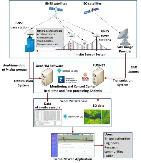
2. GeoSHM on the Forth Road Bridge

2.1. Overview of the Forth Road Bridge

Before the opening of the Queensferry Crossing in August 2017, the FRB was the major road bridge across the Firth of Forth, which links Edinburgh to Northern Scotland. When opened in 1964, this 2.5-km long bridge was the fourth longest suspension bridge in the world and the longest outside the United States of America. The 1006-m long span of the FRB is suspended from two main cables aerially spun between two 150-m high main towers. Each side span is 408 m in length. The suspended structure is made of steel trusses and features three longitudinal air gaps, with one between each footway and carriageway, and one between the two carriage ways. This perforated structure gives the FRB a strong aerodynamic stability.

The main span and two side spans were connected to the main towers by pairs of truss end links, which were among the critical elements of the FRB. In December 2015, a fracture on one of the North East truss end links connecting the main span to the North tower was detected (Figure 2). This was followed by further inspection and an approximately one-month closure of the bridge to carry out a temporary fix. Later, in February 2016, the FRB was re-opened to all traffic. A plan to prevent similar failures in the future was developed and was implemented in March 2017. Currently, all the truss end links of the main span have been replaced by truss end bearings.

On account of the steel trusses and three longitudinal air gaps, the FRB is not prone to vortex-induced vibration or flutter but is prone to buffeting due to turbulent wind, especially in the along-wind direction. On some occasions, particularly during windstorms, large response and high threat due to strong wind gusts to vehicles and the public led to the closure of the FRB. This will be discussed further in Section 3.

2.2. GeoSHM Sensor System on the Forth Road Bridge

Figure 3 describes the current status of the GeoSHM sensor system installed on the FRB. The response of the main-span is measured by three pairs of GNSS receivers. One is installed at the mid-span while the other two are installed at the navigational points (i.e., at the quarter-span points). Four of them are Leica GR10 GNSS receivers and the others are the integrated receivers developed within the GeoSHM project. The integrated receiver includes a GNSS antenna, a GNSS receiver board, and a tri-axial accelerometer inside a compact housing. There are two other Leica GNSS receivers located at the top of the North-East and South-West tower legs to monitor deformation of the main tower. A reference station is installed on the roof of the FRB control building. In the RTK mode, the horizontal and vertical accuracy of the GNSS receivers are 10 mm and 20 mm, respectively. In addition, the wind measurement is facilitated by using three Gill WindMaster 3D sonic anemometers placed at the mid-span and at the top of the two main towers. Other environmental conditions are determined by the Gill MetPak meteorological station installed at the mid span. The other key component of the GeoSHM sensor system is the EO technology. Collecting interferometric synthetic-aperture radar (InSAR) images from Sentinel-1 satellites, this technology provides remote and long-term subsidence measurement of the bridge site and its surrounding areas. Further details of the GeoSHM sensor system can be found in Reference [15].

The overview of the GeoSHM system architecture is summarised in Figure 4. Data of the GeoSHM sensor system is collected at predefined sampling frequencies and transferred to the main GeoSHM server located at the University of Nottingham for processing and storage by using a combination of optical fibres, a wireless network, and the Internet. According to the GeoSHM Data Strategy, all sensor data are divided into 10-min records and 10-min summary statistics of bridge response, loading and modal frequencies are calculated. The 10-min averaging interval was selected according to the World-Meteorological-Organisation standard so that the nature of wind such as background wind speeds and fluctuation strength can be reasonably represented by the summary statistics [38]. These summary statistics are assessed to establish the baseline performance as well as thresholds of the normal behaviour of the FRB. They are important to assist with the further structural diagnosis.

In this paper, the authors only consider selected wind and bridge performance data of the FRB collected in the two-year period from 15/10/2017 to 15/10/2019. The wind measurement is obtained from the sonic anemometer ANE3 installed at the mid-span, where 10-min mean and maximum 0.2-second gust wind speeds can be evaluated together with average wind angles measured against the positive x-axis of the bridge. The GNSS measurement is carried out using the RTK technique. From a pair of the Leica receivers SHM2 and SHM3, the lateral (along the y-axis), heaving (along the z-axis), and pitching (rotation around the x-axis) responses at the mid-span of the FRB are calculated. The 10-min means and 10-min standard deviations are obtained and represent the mean and root-mean-squared (RMS) displacement, respectively. If the former indicates the long-term or short-term quasi-static deformation of the bridge, the latter describes the dynamic characteristics of the bridge response. This is an important advantage of measuring displacement by GNSS compared to accelerations that both the mean response and dynamic components can be determined. The Ibrahim Time Domain method is then used to estimate the modal frequencies of the first lateral and heaving modes from the 10-min records of bridge response data [39]. Coordinated Universal Time (UTC) time is used in this paper.

3. Wind-Induced Effects on the Forth Road Bridge

Before the opening of the Queensferry Crossing on 30 August 2017, the FRB was the major road transportation route spanning the Firth of Forth and carrying up 65,000 vehicles per day [40]. With a high degree of flexibility, the FRB was highly susceptible to wind. The bridge performance of the FRB was also sensitive to traffic and temperature, which was found noticeable in the vertical and pitching responses, as discussed by Meng et al. in Reference [15]. Nowadays, the FRB is restricted to public buses, cyclists, and pedestrians only, and wind load becomes the dominant factor governing the bridge performance.

The wind roses in Figure 5 represent the distribution of the 10-min mean and maximum wind speed against the wind direction measured at the FRB. Thanks to its geographical location and the surrounding topography of the Firth of Forth, the FRB primarily experiences the wind between the South-West and West directions with the maximum gust speed of more than 23 ms⁻¹. Similar wind strength is also found coming from the East but is much less frequent and less dispersed. Northerly winds are very rare and have much lower strength. Figure 5 also indicates the dominance of the low wind speed for the FRB where wind records with 10-min mean speeds less than 10 ms⁻¹ are account for nearly 90% of all data.

The wind roses in Figure 6 and Figure 7 illustrate the variation of the bridge response measured at the mid-span of the FRB against the wind direction. Despite being the dominant wind, not all westerly winds are accountable for large bridge response. As shown in Figure 6, the majority of South-West winds cause very small mean lateral displacement. Strong wind from the directions that are normal to the bridge axis tends to cause larger mean and RMS lateral and heaving displacements. Figure 8 and Figure 9 describe the dependence of the lateral and heaving response on the normal component of the 10-min mean wind speed. Separating the 10-min summary statistics by the wind directions, it is evident that, compared to northerly and southerly winds, easterly and western winds cause larger normal components of the mean wind speed and induce much larger bridge response in both the lateral and heaving directions.

4. Reponses of the Forth Road Bridge during Extreme Wind Events

4.1. Extreme Windstorms

Some results presented in Section 3 showed the high susceptibility of the FRB to wind loads. Low pressure systems are a very frequent weather feature in the windstorm season, which can cause a very high risk of severe gale and rainfall to Scotland. During the GeoSHM project, there have been many instances that the FRB experienced very strong windstorms, causing significant threats not only to the bridge but also to the public and other infrastructure over significantly large areas.

Table 1. Named windstorms observed at the FRB during the GeoSHM project.

Storm Name	Date of Impact	Maximum Gust
Storm Elon	09 January 2015	113 mph (measured at Stornoway)
Storm Gertrude	29 January 2016	76 mph (measured at Inverbervie)
Storm Ali	19 September 2018	77 mph (measured at Inverbervie)

lists three named windstorms that affected the FRB during the GeoSHM project, together with the dates of impact to the UK and Northern Ireland and maximum gusts recorded.

With a recorded gust speed of approximately 120 mph, Storm Elon is one of the biggest windstorms that have affected Western and Northern Europe. Just after midnight of 09 January 2015, Storm Elon made an impact on the FRB. Analysing limited wind data provided by the bridge authority showed that the maximum gust significantly increased during a 90-second period and reached the speed of 40.7 ms⁻¹ (91 mph). The increase in the wind speed over such a short duration was similar to a step excitation on the bridge. As a result of the excitation, the non-stationary response was observed on the FRB. The mid-span was found to drift laterally to the East by 2 m, which was followed by a dynamic response at the first lateral vibration mode with the maximum peak-to-peak amplitude of 3 m. Further analysis of rainfall radar images revealed that the rapid increase in the wind speed was caused by a gust front of sustained strong winds associated with squall lines travelling across the FRB. A detailed discussion of this windstorm can be found in Reference [41]. During the storm, it was reported that a van has been blown over by a large gust of wind while crossing the bridge at 00:36, which coincided with the increase in the wind speed and bridge response (Figure 10). Incidents where vehicles were blown over on the FRB were reported on at least two other occasions, which include the dates of 11 January 2017 and 14 March 2017. These events show the vulnerability of the FRB to wind hazards and the risk to road users.

4.2. Storm Ali

Being the first storm of the 2018/2019 storm season, Storm Ali brought along very strong wind gusts measured at over 100 mph at exposed areas around the Tay Road Bridge (Scotland, UK). The widespread occurrence of strong gales and heavy rainfall caused severe damage to buildings and vehicles, extensive power outages, and travel disruption across the northwest of the UK. The storm also claimed the lives of two individuals.

As Storm Ali progressed through the north of Scotland during the morning of 19 September 2018, the GeoSHM sensor system detected an extreme wind event and was able to monitor not only the development of wind gusts around the FRB but also the variation of the bridge performance. Figure 11a,b shows the 10-min mean and maximum wind speed respectively, in the period from 15 October 2017 to 15 October 2019. Highlighted by the red circles in the figures, the peak wind speed values associated with Storm Ali occurred at 11:35 with the mean wind speed of 24 ms⁻¹ and the peak 0.2-second gust speed of 38 ms⁻¹ being recorded at the mid-span of the FRB. Further analysis of the one-hour wind record containing the peak gust speed showed that the 60-min mean wind speed was 20.4 ms⁻¹. This yields a 60-min gust factor of 1.86. Based solely on the wind speeds, it is evident that Storm Ali is the strongest windstorm observed in this period. At its peak gust speed, the average direction of the 10-min wind record is 230° and the normal component of the 10-min mean wind speed is 19.52 ms⁻¹. Despite not being the highest value in the period (Figure 11c), the normal wind speed measured during Storm Ali is still significantly larger than the 99% percentile value of 14.4 ms⁻¹ estimated from the fitted Weibull distribution, which is shown in Figure 12. This indicates the low likelihood and potentially high severity of this storm.

Examining the variation of the lateral displacement at the mid-span against the normal component of the mean wind speed (Figure 13) clearly shows the quadratic trends for all response quantities indicated by the red dashed line as predicted by the quasi-steady theory [42]. As highlighted by the red circles, the mean lateral displacement at the mid-span caused by the peak gust of Storm Ali agrees well with the quasi-steady analysis while the RMS and maximum displacements slightly deviate from the trend-lines.

As shown in Figure 14 and Figure 15, a close interrogation of the 10-min summary statistics of wind speeds and bridge response revealed that the FRB was struck by the strong wind gust of Storm Ali at 10:30 on 19 September. Following a reasonably calm early morning with the mean wind speed slowly varying around 8 ms⁻¹, the wind increases in strength from 10:15 and after 30 min reaches the mean wind speed of 19 ms⁻¹ and the gust speed of 36 ms⁻¹ at 10:55 (Figure 14). The wind speed slightly reduces and then quickly rises again reaching a higher peak at 11:45. The 24 ms⁻¹ mean wind speed and the 38 ms⁻¹ gust speed were measured. The occurrence of these two peaks of wind gusts coincide with two peaks of the lateral displacement measured at the mid-span. The second response peak is significantly larger than the first one (Figure 15). After that, the wind slowly reduces in strength toward the end of the day. This results in a slow reduction in the mean, maximum, and RMS displacement, which subside after 21:00. This marked an end to the threat of Storm Ali on the FRB.

Focusing on the two peaks of wind gusts, Figure 16 shows the time history of wind speed recorded from 09:00 to 14:00. The 1-min moving mean and maximum are included to highlight the variation of the mean wind speed and gust speed, respectively. Figure 16 confirms that the wind steadily increases in strength from 10:30 over a duration of 30 min. This causes the mid-span of the FRB to drift to the East, reaching the first response peak at around 11:00 as shown in Figure 17. Afterward, just before 11:35, the wind speed suddenly rises over a duration of 5 min. This induces a step excitation on the FRB, causing the mid-span to suddenly move to the East as shown in time histories of bridge response (Figure 17 and Figure 18). Indicated by the 1-min moving average, there is a step change in the background response, which increases by 0.8 m in 5 min. This rapid change is followed by a large dynamic response in the first lateral vibration mode with the maximum peak-to-peak amplitude of nearly 1.2 m (Figure 19).

Estimated from the 10-min records of the lateral displacement by using the Ibrahim Time Domain method, Figure 20 shows the modal frequencies of the first lateral vibration mode on 19 September. The key feature in this figure is that the frequency value significantly drops by 15% from 0.0753 Hz to 0.0644 Hz at 10:35. This sudden drop coincides with the first increase in the wind speed, as found in Figure 14 and Figure 16. After the drop, the modal frequency remains at a low value (around 0.067 Hz) and then slowly restores at 21:00 as the effect of Storm Ali on the FRB subsides. A similar relationship between the modal frequency and the wind speed is also observed in the early morning of 19 September before Storm Ali made an impact on the FRB. Plotting the modal frequency against the normal component of the mean wind speed (Figure 21) clearly shows a negative correlation between the two parameters during the period from 15 October 2017 to 15 October 2019. For the wind speed value less than 5 ms⁻¹, the average modal frequency is approximately 0.0755 Hz. As the wind speed increases to more than 15 ms⁻¹, the average modal frequency drops by 11% to approximately 0.0669 Hz. Investigating the modal frequency of the first heaving mode (Figure 22) shows a similar relationship that the frequency value reduces as the wind speed increases. It is important to note that the variation of the modal frequencies as shown in this case indicates the susceptibility of not only the bridge response but also the structural parameters of the FRB on wind loads. Understanding the dependence of the monitored parameters on wind loads and other external factors is essential to generate a baseline performance of the bridge supporting the detection of structural changes or damages. Additionally, this knowledge helps improve the structural design codes and contribute to the safety of future long-span bridges.

5. Conclusions

Using the bridge response and wind speed data collected from the GeoSHM sensor system over a two-year period (15 October 2017 to 15 October 2018), this paper has demonstrated the susceptibility of the FRB to wind loads. On 19 September 2018, an extreme wind event was alerted by the GeoSHM system when the FRB was struck by Storm Ali. During the event, the strong gust from this storm generated a step excitation on the FRB, which caused a large response at the first lateral vibration mode with the maximum peak-to-peak amplitude of approximately 1.2 m. Not only the bridge response but also the modal frequencies of the first lateral and heaving modes were found dependent on the wind speed such that, as the wind speed increases, the frequency value decreases. For the first lateral mode, an 11% reduction in the modal frequency was observed. The paper showed the benefit of using the GeoSHM system to monitor the performance of the FRB during extreme wind events, particularly the capability of the GNSS receivers to measure both the quasi-static and dynamic responses of the bridge. Analysing the bridge response and wind data collected during such events can help understand better the performance of the monitored structure under different loading conditions. In addition, the knowledge derived from the data can enable further understanding of the nature of wind and wind-structure interaction, and improve wind loading models that are currently used in international and national design codes. This will contribute to enhancing the resilience of current and future infrastructure in extreme wind events, which are becoming more frequent and severe with climate change.

References

1. Failure Knowledge Database. Available online: www.shipai.org/fkd/en/cfen/CD1000144.html (accessed on 17 May 2018).
2. Liao, M.; Okazaki, T.A. Computational Study of the I-35W Bridge Collapse (CTS 09-20); Research Report for Centre for Transportation Studies; University of Minnesota: Minneapolis, MN, USA, October 2009. [Google Scholar]
3. The Guardian. Available online: www.theguardian.com/cities/2019/feb/26/what-caused-the-genoa-morandi-bridge-collapse-and-the-end-of-an-italian-national-myth (accessed on 22 October 2019).
4. New Civil Engineer. Available online: www.newcivilengineer.com/latest/fatal-taiwan-bridge-collapse-is-latest-example-of-maintenance-failings-07-10-2019 (accessed on 15 October 2019).
5. New Civil Engineer. Available online: www.newcivilengineer.com/latest/work-begins-on-hammersmith-bridge-as-120m-repair-bill-announced-05-09-2019 (accessed on 15 October 2019).
6. Meng, X. Real-time Deformation Monitoring of Bridges using GPS/Accelerometers. Ph.D. Thesis, University of Nottingham, Nottingham, UK, May 2002. [Google Scholar]
7. Nickitopoulou, A.; Protopsalti, K.; Stiros, S. Monitoring dynamic and quasi-static deformations of large flexible engineering structures with GPS: Accuracy, limitations and promises. Eng. Struct. 2006, 28, 1471–1482. [Google Scholar] [CrossRef]
8. Im, S.B.; Hurlebaus, S.; Kang, Y.J. Summary review of GPS technology for structural health monitoring. J. Struct. Eng. 2013, 139, 1653–1664. [Google Scholar] [CrossRef]
9. Xu, L.; Guo, J.; Jiang, J. Time-frequency analysis of a suspension bridge based on GPS. J. Sound Vib. 2002, 245, 105–116. [Google Scholar] [CrossRef]
10. Meng, X.; Dodson, A.; Roberts, G. Detecting bridge dynamics with GPS and triaxial accelerometers. Eng. Struct. 2007, 29, 3178–3184. [Google Scholar] [CrossRef]
11. Watson, C.; Watson, T.; Coleman, R. Structural monitoring of cable-stayed bridges: Analysis of GPS versus modeled deflections. J. Surv. Eng. 2007, 133, 23–28. [Google Scholar] [CrossRef]
12. Psimoulis, P.; Pytharouli, S.; Karambalis, D.; Stiros, S. Potential of global positioning system (GPS) to measure frequencies of oscillations of engineering structures. J. Sound Vib. 2008, 318, 606–623. [Google Scholar] [CrossRef]
13. Roberts, G.W.; Brown, C.J.; Atkins, C.; Meng, X.; Colford, B.; Ogundipe, O. Deflection and frequency monitoring of the Forth Road Bridge, Scotland, by GPS. Proc. Inst. Civ. Eng. Bridge Eng. 2012, 165, 105–123. [Google Scholar] [CrossRef]
14. Yu, J.; Meng, X.; Shao, X.; Yan, B.; Yang, L. Identification of dynamic displacements and model frequencies of a medium-span suspension bridge using multimode GNSS processing. Eng. Struct. 2014, 81, 432–443. [Google Scholar] [CrossRef]
15. Meng, X.; Nguyen, D.T.; Xie, Y.; Owen, J.S.; Psimoulis, P.; Ince, S.; Chen, Q.; Ye, J.; Bhatia, P. Design and implementation of a new system for large bridge monitoring—GeoSHM. Sensors 2018, 18, 775. [Google Scholar] [CrossRef]
16. Meng, X.; Roberts, G.W.; Dodson, A.; Cosser, E.; Barnes, J.; Rizos, C. Impact of GPS satellite and pseudolite geometery on structural deformation monitoring: Analytical and empirical studies. J. Geod. 2004, 77, 809–822. [Google Scholar] [CrossRef]
17. Kijewski-Correa, T.; Kochly, M. Monitoring the wind-induced response of tall buildings: GPS performance and the issue of multipath effects. J. Wind. Eng. Ind. Aerodyn. 2007, 95, 1176–1198. [Google Scholar] [CrossRef]
18. Moschas, F.; Stiros, S. Dynamic multipath in structural bridge monitoring: An experimental approach. GPS Solut. 2014, 18, 209–218. [Google Scholar] [CrossRef]
19. Gao, W.; Meng, X.; Gao, C.; Pan, S.; Zhu, Z.; Xia, Y. Analysis of the carrier-phase multipath in GNSS triple-frequency observation combinations. Adv. Space Res. 2019, 63, 2735–2744. [Google Scholar] [CrossRef]
20. Roberts, G.W.; Cosser, E.; Meng, X.; Dodson, A. High frequency deflection monitoring of bridges by GPS. J. Glob. Position. 2004, 3, 226–231. [Google Scholar] [CrossRef]
21. Tamura, Y.; Matui, M.; Panini, L.-C.; Ishibashi, R.; Yoshida, A. Measurement of wind-induced response of buildings using RTK-GPS. J. Wind Eng. Ind. Aerodyn. 2002, 90, 1783–1793. [Google Scholar] [CrossRef]
22. Brownjohn, J.W.M.; Stringer, M.; Tan, G.; Poh, Y.K.; Ge, L.; Pan, T.C. Experience with RTK-GPS system for monitoring wind and seismic effects on a tall building. In Proceedings of the 2nd International Conference on Structural Health Monitoring of Intelligent Infrastructure, Shenzhen, China, 16–18 November 2005. [Google Scholar]
23. Owen, J.S.; Nguyen, D.T.; Meng, X.; Xie, Y.; Psimoulis, P. The influence of uncertainty in wind field parameters on predicted buffeting response of bridges. In Proceedings of the 15th International Conference on Wind Engineering, Beijing, China, 1–6 September 2019. [Google Scholar]
24. Moschas, F.; Stiros, S. Measurement of the dynamic displacements and of the modal frequencies of a short-span pedestrian bridges using GPS and an accelerometer. Eng. Struct. 2011, 33, 10–17. [Google Scholar] [CrossRef]
25. Li, X.; Ge, L.; Ambikairajah, E.; Rizos, C.; Tamura, Y.; Yoshida, A. Full-scale structural monitoring using an intergrated GPS and accelerometer system. GPS Solut. 2006, 10, 233–247. [Google Scholar] [CrossRef]
26. Xiong, C.; Lu, H.; Zhu, J. Operational model analysis of bridge structures using data from GNSS/accelerometer measurements. Sensors 2017, 17, 436. [Google Scholar] [CrossRef]
27. Meng, X.; Wang, J.; Han, H. Optimal GPS/accelerometer integration algorithm for monitoring the vertical structural dynamics. J. Appl. Geod. 2014, 8, 265–272. [Google Scholar] [CrossRef]
28. Han, H.; Wang, J.; Meng, X.; Lui, H. Analysis of the dynamic response of a long span bridge using GPS/accelerometer/anemometer under typhoon loading. Eng. Struct. 2016, 122, 238–250. [Google Scholar] [CrossRef]
29. Chan, T.H.; Yu, L.; Tam, H.Y.; Ni, Y.Q.; Liu, S.; Chung, W.; Cheng, L. Fiber bragg grating sensor for structural health monitoring of Tsing Ma Bridge: Background and experimental observation. Eng. Struct. 2006, 28, 648–659. [Google Scholar] [CrossRef]
30. Xu, Y.L.; Xia, Y. Structural Health Monitoring of Long-Span Suspension Bridges; CRC Press: Boca Raton, FL, USA, 2011. [Google Scholar]
31. Andersen, E.; Pederson, L. Structural monitoring of the Great Belt East Bridge. Strait Crossings 1994, 94, 189–195. [Google Scholar]
32. Wang, H.; Tao, T.; Li, A.; Zhang, Y. Structural health monitoring system for Sutong cable-stayed bridge. Smart Struct. Syst. 2016, 18, 317–334. [Google Scholar] [CrossRef]
33. Laory, I.; Ali, N.B.; Trinh, T.N.; Smith, I.F.C. Measurement system configuration for damage identification of continuously monitored structures. J. Bridge Eng. 2012, 17, 857–866. [Google Scholar] [CrossRef]
34. Dervilis, N.; Worden, K.; Crosss, E.J. On robust regression analysis as a means of exploring environmental and operational conditions of SHM data. J. Sound Vib. 2015, 347, 279–296. [Google Scholar] [CrossRef]
35. Cross, E.J.; Koo, K.Y.; Brownjohn, J.M.W.; Worden, K. Long-term monitoring and data analysis of the Tamar Bridge. Mech. Syst. Signal Process. 2013, 35, 16–34. [Google Scholar] [CrossRef]
36. Chen, Q.; Jiang, W.; Meng, X.; Jiang, P.; Wang, K.; Xie, Y.; Ge, Y. Vertical deformation monitoring of the suspension bridge tower using GNSS: A case study of the Forth Road Bridge in the UK. Remote Sens. 2018, 10, 364. [Google Scholar] [CrossRef] [Green Version]
37. Roberts, G.W.; Meng, X.; Psimoulis, P.; Brown, C.J. Time series analysis of rapid GNSS measurements for quasi-static and dynamic bridge monitoring. In Geodetic Time Series Analysis in Earth Sciences; Montillet, J.P., Bos, M., Eds.; Springer Geophysics: Cham, Switzerland, 2019; pp. 345–417. [Google Scholar]
38. World Meteorological Organization. Guidelines for Converting Between Various Wind Averaging Periods in Tropical Cyclone Conditions; World Meteorological Organization: Geneva, Switzerland, 2010. [Google Scholar]
39. Ewins, D.J. Modal Testing: Theory, Practice and Application, 2nd ed.; Research Studies Press: Baldock, UK, 2000. [Google Scholar]
40. 3 Centuries of Spanning the Forth. Available online: web.archive.org/web/20130606162211/http://www.transportscotland.gov.uk/files/documents/projects/forth-replacement/Forth_Bridge_Brochure_VisFinal.pdf (accessed on 24 October 2019).
41. Owen, J.S.; Nguyen, D.T.; Meng, X.; Psimoulis, P.; Xie, Y. The application of rainfall radar to interpret non-stationary wind effects on the Forth Road Bridge. In Proceedings of the 13th UK Conference on Wind Engineering, Leeds, UK, 3–4 September 2018. [Google Scholar]
42. Simiu, E.; Scanlan, R. Wind Effects on Structures: Fundamentals and Application to Design, 3rd ed.; Wiley: New York, NY, USA, 1996. [Google Scholar]
Figure 1. (a) The Forth Road Bridge (Edinburgh, UK) (Stuart Halliday/CC-BY-3.0), (b) the Wuhu Yangtze Bridge (Wuhu, China) (Glabb/CC-BY-SA-3.0), and (c) the Ningbo Zhaobaosang Bridge (Ningbo, China).
Remotesensing 11 02799 g001
Figure 2. Fractured North East truss end link (www.civilengineer.com).
Remotesensing 11 02799 g002
Figure 3. (a) GeoSHM sensor system and (b) the coordinate system of the FRB.
Remotesensing 11 02799 g003
Figure 4. Overall GeoSHM system architecture showing the data flow between the sub-systems.
Remotesensing 11 02799 g004
Figure 5. Wind roses of (a) the 10-min mean wind speed and (b) the maximum 0.2-second gust wind speed. The x-axis of the bridge is aligned with the red lines.
Remotesensing 11 02799 g005
Figure 6. Wind rose of the mean lateral response. The x-axis of the bridge is aligned with the red line.
Remotesensing 11 02799 g006
Figure 7. Wind roses of (a) the RMS lateral response and (b) the RMS heaving response. The x-axis of the bridge is aligned with the red lines.
Remotesensing 11 02799 g007
Figure 8. Variability of the mean lateral response against the normal component of the 10-min mean wind speed.
Remotesensing 11 02799 g008
Figure 9. Variability of (a) the RMS lateral response and (b) the RMS heaving response against the normal component of the 10-min mean wind speed.
Remotesensing 11 02799 g009
Figure 10. A van blown over on the FRB at 00:36 on 09 January 2015 (www.pressandjournal.co.uk).
Remotesensing 11 02799 g010
Figure 11. (a) The 10-min mean wind speed, (b) the maximum 0.2-second gust wind speed, and (c) the normal component of the mean wind speed in the duration from 15/10/2017 to 15/10/2019. Storm Ali is highlighted by the red circle.
Remotesensing 11 02799 g011
Figure 12. (a) The full and (b) close-up view of the cumulative distribution of the normal component of the 10-min mean wind speed, compared against the fitted Weibull distribution (the distribution parameters are A = 6.280, B = 1.838). The black line indicates the 99% percentile value of 14.4 ms−1.
Remotesensing 11 02799 g012
Figure 13. Variation of (a) the mean, (b) RMS, and (c) maximum lateral displacement against the normal component of the 10-min mean wind speed. The data points on 19 September 2018 are shown in green while the ones associated with the peak wind speeds due to Storm Ali are highlighted by the red circles.
Remotesensing 11 02799 g013aRemotesensing 11 02799 g013b
Figure 14. 24-h variation of the 10-min mean and maximum wind speed on 19 September 2018. Data points are joined for better clarification.
Remotesensing 11 02799 g014
Figure 15. 24-h record of (a) the mean and maximum lateral displacement and (b) the RMS lateral displacement at the mid-span of the FRB on 19/09/2018. Data points are joined for better clarification. The negative values of the mean and maximum response on the sub-figure (a) represent the movement to the East of the mid-span (i.e., towards the negative y-axis indicated in Figure 3) due to the effect of Westerly winds.
Remotesensing 11 02799 g015
Figure 16. Wind speed recorded at the mid-span of the FRB from 09:00 to 14:00 on 19 September 2018.
Remotesensing 11 02799 g016
Figure 17. Lateral displacement at the mid-span of the FRB from 09:00 to 14:00 on 19 September 2018.
Remotesensing 11 02799 g017
Figure 18. Lateral displacement at the mid-span of the FRB from 11:15 to 12:15 on 19 September 2018.
Remotesensing 11 02799 g018
Figure 19. Dynamic component of the lateral displacement at the mid-span of the FRB from 11:15 to 12:15 on 19 September 2018.
Remotesensing 11 02799 g019
Figure 20. 24-h variation of the modal frequency of the first lateral model on 19 September 2018. Data points are joined for better clarification.
Remotesensing 11 02799 g020
Figure 21. Variation of the modal frequency of the first lateral mode against the normal component of the 10-min mean wind speed. Data points of 19 September 2018 are highlighted in red.
Remotesensing 11 02799 g021
Figure 22. Variation of the modal frequency of the first heaving mode against the normal component of the 10-min mean wind speed. Data points of 19 September 2018 are highlighted in red.
Remotesensing 11 02799 g022